| Issue |
A&A
Volume 667, November 2022
|
|
|---|---|---|
| Article Number | A8 | |
| Number of page(s) | 21 | |
| Section | Planets and planetary systems | |
| DOI | https://doi.org/10.1051/0004-6361/202244079 | |
| Published online | 31 October 2022 | |
The GAPS programme at TNG
XL. A puffy and warm Neptune-sized planet and an outer Neptune-mass candidate orbiting the solar-type star TOI-1422
1
Department of Physics, University of Rome “Tor Vergata”,
Via della Ricerca Scientifica 1,
00133
Rome, Italy
e-mail: This email address is being protected from spambots. You need JavaScript enabled to view it.
2
Department of Physics and Astronomy, University of Florence,
Largo Enrico Fermi 5,
50125
Firenze, Italy
3
INAF – Turin Astrophysical Observatory,
via Osservatorio 20,
10025
Pino Torinese, Italy
4
Max Planck Institute for Astronomy,
Königstuhl 17,
69117
Heidelberg, Germany
5
INAF – Osservatorio Astronomico di Roma,
via Frascati 33,
00040
Monte Porzio Catone (RM), Italy
6
Aix-Marseille Université, CNRS, CNES, LAM,
Marseille, France
7
INAF – Osservatorio Astronomico di Padova,
Vicolo dell’Osservatorio 5,
35122
Padova, Italy
8
Dipartimento di Fisica, Universitá degli Studi di Torino,
via Pietro Giuria 1,
10125
Torino, Italy
9
Centro de Astrobiología, Depto. de Astrofísica,
ESAC campus,
28692,
Villanueva de la Cañada (Madrid), Spain
10
Center for Astrophysics | Harvard & Smithsonian,
60 Garden Street,
Cambridge, MA
02138, USA
11
Department of Earth and Planetary Sciences, Harvard University,
20 Oxford Street,
Cambridge, MA
02138, USA
12
INAF – Osservatorio Astronomico di Trieste,
via Tiepolo 11,
34143
Trieste, Italy
13
INAF – Osservatorio Astronomico di Capodimonte,
Salita Moiariello 16,
80131
Naples, Italy
14
INAF – Osservatorio Astrofísico di Catania,
via S. Sofia 78,
95123
Catania, Italy
15
INAF – Osservatorio Astronomico di Palermo,
Piazza del Parlamento 1,
90134
Palermo, Italy
16
INAF – Osservatorio Astronomico di Cagliari,
via della Scienza 5,
09047
Selargius (CA), Italy
17
Dipartimento di Fisica e Astronomia “Galileo Galilei” – Università di Padova,
Vicolo dell’Osservatorio 2,
35122
Padova, Italy
18
INAF – Osservatorio Astronomico di Brera,
Via E. Bianchi 46,
23807
Merate (LC), Italy
19
Fundación Galileo Galilei – INAF,
Rambla José Ana Fernandez Pérez 7,
38712
Brena Baja, TF, Spain
20
European Southern Observatory,
Karl-Schwarzschild-Straße 2,
85748
Garching, Germany
21
Institut d’Astrophysique de Paris, CNRS, UMR 7095 & Sorbonne Université,
UPMC Paris 6, 98bis Bd Arago,
75014
Paris, France
22
Observatoire de Haute-Provence, CNRS, Université d’Aix-Marseille,
04870
Saint-Michel-l’Observatoire, France
23
Aix-Marseille Université, CNRS, CNES, LAM,
Marseille, France
24
Université Grenoble Alpes, CNRS, IPAG,
38000
Grenoble, France
25
Department of Physics, Shahid Beheshti University,
Tehran, Iran
26
Laboratoire J.-L. Lagrange, OCA, Université de Nice-Sophia Antipolis, CNRS,
Campus Valrose,
06108
Nice Cedex 2, France
27
IRAP, Université de Toulouse, CNRS, UPS, CNES,
31400
Toulouse, France
28
Department of Physics and Kavli Institute for Astrophysics and Space Research, Massachusetts Institute of Technology,
Cambridge, MA
02139, USA
29
NASA Goddard Space Flight Center,
8800 Greenbelt Road,
Greenbelt, MD
20771, USA
30
Department of Earth, Atmospheric and Planetary Sciences, Massachusetts Institute of Technology,
Cambridge, MA
02139, USA
31
Kavli Institute for Astrophysics and Space Research, Massachusetts Institute of Technology,
Cambridge, MA
02139, USA
32
Harvard-Smithsonian Center for Astrophysics,
60 Garden Street,
Cambridge, MA
02138, USA
33
Department of Physics and Astronomy, University of New Mexico,
210 Yale Blvd NE,
Albuquerque, NM
87106, USA
34
NASA Ames Research Center,
Moffett Field, CA
94035, USA
35
SETI Institute,
Mountain View, CA
94043, USA
36
Space Science & Astrobiology Division MS 245-3, NASA Ames Research Center,
Moffett Field, CA
94035, USA
37
INAF-Telescopio Nazionale Galileo,
Apartado 565,
38700,
Santa Cruz de La Palma, Spain
38
Department of Astrophysical Sciences, Princeton University,
Princeton, NJ
08544, USA
39
Astrophysics Group, Keele University,
Staffordshire
ST5 5BG, UK
40
Department of Aeronautics and Astronautics, MIT,
77 Massachusetts Avenue,
Cambridge, MA
02139, USA
Received:
21
May
2022
Accepted:
7
July
2022
Abstract
Context. Neptunes represent one of the main types of exoplanets and have chemical-physical characteristics halfway between rocky and gas giant planets. Therefore, their characterization is important for understanding and constraining both the formation mechanisms and the evolution patterns of planets.
Aims. We investigate the exoplanet candidate TOI-1422 b, which was discovered by the TESS space telescope around the high proper-motion G2 V star TOI-1422 (V = 10.6 mag), 155 pc away, with the primary goal of confirming its planetary nature and characterising its properties.
Methods. We monitored TOI-1422 with the HARPS-N spectrograph for 1.5 yr to precisely quantify its radial velocity (RV) variation. We analyse these RV measurements jointly with TESS photometry and check for blended companions through high-spatial resolution images using the AstraLux instrument.
Results. We estimate that the parent star has a radius of R⋆ = 1.019−0.013+0.014 R⊙, and a mass of M⋆ = 1.019−0.013+0.014 M⊙. Our analysis confirms the planetary nature of TOI-1422 b and also suggests the presence of a Neptune-mass planet on a more distant orbit, the candidate TOI-1422 c, which is not detected in TESS light curves. The inner planet, TOI-1422 b, orbits on a period of Pb = 12.9972 ± 0.0006 days and has an equilibrium temperature of Teq,b = 867 ± 17 K. With a radius of Rb = 3.96−0.11+0.13 R⊕, a mass of Mb = 9.0−2.0+2.3 M⊕ and, consequently, a density of ρb = 0.795−0.235+0.290g cm−3, it can be considered a warm Neptune-sized planet. Compared to other exoplanets of a similar mass range, TOI-1422 b is among the most inflated, and we expect this planet to have an extensive gaseous envelope that surrounds a core with a mass fraction around 10% – 25% of the total mass of the planet. The outer non-transiting planet candidate, TOI-1422 c, has an orbital period of Pc = 29.29−0.20+0.21 days, a minimum mass, Mcsin i, of 11.1−2.3+2.6 M⊕, an equilibrium temperature of Teq,c = 661 ± 13 K and, therefore, if confirmed, could be considered as another warm Neptune.
Key words: techniques: photometric / planetary systems / techniques: spectroscopic / techniques: radial velocities / stars: individual: TOI-1422 / methods: data analysis
© L. Naponiello et al.
 Open Access article, published by EDP Sciences, under the terms of the Creative Commons Attribution License (https://creativecommons.org/licenses/by/4.0), which permits unrestricted use, distribution, and reproduction in any medium, provided the original work is properly cited.
This article is published in open access under the Subscribe-to-Open model. This email address is being protected from spambots. You need JavaScript enabled to view it. to support open access publication.
1 Introduction
Exoplanetary science has expanded quickly from the simple detection of new worlds to their in-depth characterization. This characterization is especially feasible for planets orbiting bright stars on a plane almost aligned to our line of sight, meaning that their radius and mass can be derived by transit photometry and radial velocity (RV) measurements, respectively. The population of known transiting planets has increased significantly in the last two decades, mainly thanks to dedicated ground-based surveys, which were then followed by surveys from space that turned out to be much more efficient, considering the total number of discoveries.
Thus far, the Kepler and the K2 space missions (Borucki et al. 2010; Howell et al. 2014) have had a very important impact on the exoplanet field by discovering thousands of confirmed and candidate planets, many of which are not amenable to RV follow-up due to the faintness of their host stars. The Transiting Exoplanet Survey Satellite (TESS; Ricker et al. 2014), currently at the end of its first extended mission and with a second one already proposed, was designed to target nearby and bright stars over a large portion of the sky (around 85% sky coverage during the primary mission alone) because such stars are easier to follow up by means of RV, and result in refined measurements of their own exoplanet masses, atmospheres, sizes, and therefore, densities. The opportunity to use a large exoplanet sample such as that of Kepler, which is based on homogeneous data and has minimal pollution from false positives (< 10%, Fressin et al. 2013), has allowed us to distinguish between several distinct exoplanet regimes (Weiss & Marcy 2014; Buchhave et al. 2014; Zeng et al. 2019): the terrestrial-like planets (Rp < 1.7 R⊙), the gas dwarf planets with rocky cores and hydrogen-helium envelopes, the H2O-dominated ices and fluid water worlds (both of the latter two classes have 1.7R⊕ < Rp < 3.9R⊕) and the ice or gas giant planets (Rp > 3.9R⊕).
Planet occurrence around main-sequence stars has been investigated thanks to Doppler surveys (e.g. Cumming et al. 2008; Wright et al. 2012). In particular, the Keck Eta-Earth survey (Howard et al. 2010) and the CORALIE+HARPS survey (Mayor et al. 2011) first explored the domain of low-mass (3–30 M⊕) close-in (Porb ~ 50 days) planets. These planets turned out to be an order of magnitude more common than giant planets.
Other studies for determining the occurrence rates of planets, based on the Kepler sample, agree that for planets with less than a 1-yr orbital period, their mean number per star is higher within the radius range 1 R⊕ < Rp < 4 R⊕ rather than the range 4R⊕ < Rp < 16R⊕, (Howard et al. 2012; Fressin et al. 2013; Petigura et al. 2013). The subsequent and gradual refinement of parent-star properties (especially thanks to high-resolution stellar spectra) revealed a clear bimodality of the radius distribution of close-in (P < 100 days), small-sized (Rp < 4.0 R⊕) planets orbiting bright, main-sequence solar-type stars (Petigura et al. 2017; Fulton & Petigura 2018; Van Eylen et al. 2018)1. These two quite distinct populations were identified as ‘super-Earths’ (Rp < 1.5 R⊕) and ‘sub-Neptunes’ (Rp = 2–3 R⊕), which are also represented in the intermediate region (Rp = 1.5–2 R⊕) with fewer planets. However, it is better to stress that, since we do not know for sure what they are made of, the space of physical parameters (Rp, Mp), for which the previous terms apply, are not strictly defined.
The advantage of studying transiting planets is the possibility, in many cases, to measure both the planetary radius and mass, and therefore determine their density and bulk composition. Knowing the structural properties, one should be able to distinguish among the various scenarios of exoplanet formation and evolution. Unfortunately, theoretical models (e.g. Bitsch et al. 2019; Turbet et al. 2020) tell us that the mass-radius relationships for small planets present degeneracy due to the vastness of possible different compositions and amounts of rock, ice, and gas, especially in the transition between rocky super-Earths and Neptune-like planets (e.g. Miller-Ricci et al. 2009; Lozovsky et al. 2018). A detailed investigation of the mass-radius relation for small planets can be useful for throwing light on several open questions, such as the diversity of planet core masses and compositions, or where they form (in situ or beyond the snowline), and the existence of the radius gap. We refer the reader to the recent review by Biazzo et al. (2022) for an exhaustive discussion on this topic.
It is therefore clear how RV follow-up observations and planetary-mass measurements play an important role in understanding this process and why there is currently a tremendous effort in this field by many teams (e.g. KESPRINT: Gandolfi et al. 2018; HARPS-N consortium: Cloutier et al. 2020; NCORES: Armstrong et al. 2020; TESS-Keck Survey: Chontos et al. 2022; GAPS: Carleo et al. 2021) to confirm TESS small-planet candidates.
Probing the chemical composition of the atmosphere of a large number of sub-Neptune planets would also be helpful to unravel the skein. Various techniques (such as high-resolution spectroscopy, transmission, and emission spectroscopy) have been implemented and applied successfully using the Hubble Space Telescope (HST) instruments or the high-resolution spectrographs mounted on large-class ground-based telescopes (e.g. CRIRES: Snellen et al. 2010; HARPS: Wyttenbach et al. 2015; LDSS3C: Diamond-Lowe et al. 2018; GIANO: Brogi et al. 2018; CARMENES: Casasayas-Barris et al. 2019; HARPS-N: Pino et al. 2020; ESPRESSO: Borsa et al. 2021). Unfortunately, these techniques for probing the planetary atmospheres are currently effectively applicable only to giant planets, as we know only a few sub-Neptune planets for which the transmission-spectrum signal can be detected with a sufficient signal-to-noise ratio (S/N) that allows us to discriminate between different atmospheric models. The featureless transmission spectra of GJ 436 b (Knutson et al. 2014) and GJ 1214 b (Kreidberg et al. 2014) are emblematic.
The situation should improve soon thanks to the James Webb Space Telescope (JWST; Barstow et al. 2015), which is about to go into operation, and with the next generation of space-based and large ground-based telescopes (Ariel: Tinetti et al. 2021; ELT: Ramsay et al. 2021; TMT: Skidmore et al. 2015). In the meantime, it is important that we continue to work to uncover new exoplanets, especially those of small size (Rp < 5 R⊕) that orbit bright (V < 11 mag) main-sequence dwarf stars. This is currently possible thanks to the large number of planet candidates (more than 5000) that TESS is discovering at the present time. The recent detection of water vapour in the atmosphere of the super-Neptune TOI-674b with the HST (Brande et al. 2022) is a successful example of this effort.
On the 6 November 2019, the TESS target star TIC 333473672 was officially named TOI-1422 (TESS Object of Interest; Guerrero et al. 2021), following the Data Validation Report Summary (DRS) produced by the TESS Science Processing Operations Center (SPOC; Jenkins et al. 2016) pipeline at the NASA Ames Research Center through the Transiting Planet Search (TPS; Jenkins 2002; Jenkins et al. 2010, 2020) and Data Validation (DV; Twicken et al. 2018, Li et al. 2019) modules. In particular, TOI-1422 01 was flagged as a potential planet with an orbital period of 13.0020 ± 0.0040 days, a transit depth of 1422 ± 94 ppm (parts per million), and a corresponding radius of 3.85 ± 0.90 R⊕, which is compatible with Neptune’s radius. The candidate passed all SPOC DV diagnostic tests, and, furthermore, all TIC (version 8) objects other than the target star were excluded as sources of the transit signal through the difference image centroid offsets (Twicken et al. 2018).
The long-term, multi-programme Global Architecture of Planetary Systems (GAPS; Covino et al. 2013; Poretti et al. 2016) exploits Doppler measurements taken with the High Accuracy Radial velocity Planet Searcher for the Northern hemisphere (HARPS-N; Cosentino et al. 2012) instrument at the Telescopio Nazionale Galileo (TNG) in La Palma (Spain). This high-resolution spectrograph (resolving power R ≈ 115 000) delivers the highest RV precision (~1 m s−1) currently achievable in the northern hemisphere. One of the aims of the GAPS programme is to confirm and obtain an accurate mass determination of planets having an intermediate-mass between super-Earths and super-Neptunes; for this reason, TOI-1422 was selected for RV follow-up observations, which started in June 2020.
In the present work, we report the results of our measurements and analyses that allowed us to confirm TOI-1422 as a new planetary system. The paper is organized as follows: Sect. 2 contains the details of the instruments, and the photometric and RV measurements; the results of our analyses are presented in Sect. 3 and discussed in Sect. 4; and we finally address the conclusions in Sect. 5.
2 Observations and data reduction
2.1 TESS photometry
Since late July 2018, TESS has observed more than 200 000 stars with its four wide-field optical Charged-Coupled Devices (CCD) cameras (24 × 96 degrees), each having a focal ratio of f / 1.4 and a broad-band filter range between 600 and 1000 nm. The pre-selected target TIC 333473672 was observed in Sectors 16 and 17 between 11 September 2019 and 2 November 2019, and the first of a total of four transiting events were recorded on 19 September 2019. The two-minute cadence photometry of TOI-1422 from TESS spans a total of ≈ 50 days and to analyse it, we used the Presearch Data Conditioning Simple Aperture Photometry (PDC-SAP; Stumpe et al. 2012, 2014, Smith et al. 2012) light curve, which is provided by the TESS SPOC pipeline and retrieved through the Python package lightkurve (Lightkurve Collaboration 2018) from the Mikulski Archive for Space Telescopes (MAST). We jointly fitted the transit model and a Gaussian process (GP) using a simple (approximate) Matern kernel, which was implemented in the Python modelling tool juliet2 (Espinoza et al. 2019) via celerite (Foreman-Mackey et al. 2017), of the form:
 (1)
(1)
where σi is the error bar of the i-th data point, σGP the amplitude of the GP in parts per million (ppm), σw an added jitter term (in ppm), δi,j the Kronecker’s delta, k(τi,j) the element i, j of the covariance matrix as a function of τi,j = |ti − tj|, with ti and tj being the i, j GP regressors (i.e. the observing times), while
![Mathematical equation: $M\left( {{\tau _{i,j,\rho }}} \right) = \left( {1 + 1{\rm{/}}} \right){{\rm{e}}^{ - \left[ {1 - } \right]\sqrt 3 {\tau _{i,j/\rho }}}} + \left( {1 - 1{\rm{/}}} \right){{\rm{e}}^{ - \left[ {1 + } \right]\sqrt 3 {\tau _{i,j/\rho }}}}$](/articles/aa/full_html/2022/11/aa44079-22/aa44079-22-eq9.png) (2)
(2)
is the kernel with its characteristic time scale ρ. The parameter є controls the quality of the approximation since, in the limit є → 0, Eq. (2) becomes the Matern-3/2 function. In juliet, the possible polluting sources inside the TESS aperture3 (Fig. 1), which might result in a smaller transit depth compared to the real one, are taken into account with a dilution factor (D) that, in this case, has been neglected because the PDC-SAP photometry is already corrected for dilution from other objects contained within the aperture using the Create Optimal Apertures (COA) module (Bryson et al. 2010, 2020)4. In order to efficiently sample the whole plausible zone in the (b, k) plane, where b is the impact parameter and k is the planet-to-star radius ratio, we used the (r1, r2) parametrization described in Espinoza (2018). This is the same approach that we adopted for the modelling of the transits in the joint analysis with the RVs (see Sect. 3.3). Moreover, here we make use of the limb-darkening parametrizations of Kipping (2013) for two-parameter limb-darkening laws (q1, q2 → u1, u2).
The PDC-SAP light curve of TOI-1422 and its detrending are plotted in Fig. 2. We also analysed the SPOC SAP photometry (Twicken et al. 2010; Morris et al. 2020), which presents a small long-term variability that might be due to systematics, but no other feature or modulation can be discerned within the experimental uncertainties, aside from a possible single extra transit event, which is discussed at the end of Sect. 3.4, and a steep flux drop at the end of both the SAP and PDC-SAP light curves, which are probably due to high levels of background noise.
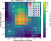 |
Fig. 1 Target pixel file from the TESS observation of Sector 16, made with tpfplotter (Aller et al. 2020) and centred on TOI-1422, which is marked with a white cross. The SPOC pipeline aperture is shown by shaded red squares, and the Gaia satellite eDR3 catalogue (Brown et al. 2018; Prusti et al. 2016) is also overlaid with symbol sizes proportional to the magnitude difference with TOI-1422. The difference image centroid locates the source of the transits within 1.89 ± 5 arcsec of the target star’s location, as reported by the TicOffset for the multi-sector DV report for this system. |
2.2 High-spatial resolution imaging – AstraLux
We observed TOI-1422 with the AstraLux high-spatial resolution camera (Hormuth et al. 2008), located at the 2.2 m telescope of the Calar Alto Observatory (CAHA, Almería, Spain) using the lucky-imaging technique. This technique obtains diffraction-limited images by acquiring thousands of short-exposure frames and selecting those with the highest Strehl ratio (Strehl 1902) to finally combine them into a co-added high-spatial resolution image. We observed this target on the night of 29 September 2021 under good weather conditions with a mean seeing of 1 arcsec, and obtained 50 000 frames with 20 ms exposure time in the Sloan Digital Sky Survey z filter (SDSSz), with a field of view windowed to 6 × 6 arcsec. The datacube was reduced by the instrument pipeline (Hormuth et al. 2008) and we selected the best quality 10% frames to produce the final high-resolution image. We obtained the sensitivity limits of the co-added image by using our own developed ASTRASENS package5 with the procedure described in Lillo-Box et al. (2012, 2014). The 5σ sensitivity curve is shown in Fig. 3. We could discard sources down to 0.2 arcsec with a magnitude contrast of ∆Z < 4 mag, corresponding to a maximum contamination level of 2.5%. By using this high-spatial resolution image, we also estimated the probability of an undetected blended source. This probability (fully described in Lillo-Box et al. 2014) is called the blended source confidence (BSC). We used a python implementation of this approach (bsc, by J. Lillo-Box), which uses the TRILEGAL6 galactic model (v1.6; Girardi et al. 2012) to retrieve a simulated source population of the region around the corresponding target7. This simulated population was used to compute the density of stars around the target position (radius r = 1°) and derive the probability of chance alignment at a given contrast magnitude and separation. When applied to the TOI-1422 location, we used a maximum contrast magnitude of ∆mb,max = 6.97 mag in the SDSSz passband, corresponding to the maximum contrast of a blended eclipsing binary that could mimic the observed transit depth of planet b (~ 1000 ppm). Thanks to our high-resolution image, we estimated the probability of an undetected blended source to be 0.28%. The probability of such an undetected source being an appropriate eclipsing binary was thus even lower and consequently, we could assume that the transit signal was not due to a blended eclipsing binary.
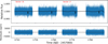 |
Fig. 2 Light curve of TOI-1422 as collected by TESS in Sectors 16 and 17 with a 2-min cadence. Top panel: light curve from the PDC-SAP pipeline. The black line represents the best-fit model obtained through GP detrending, as detailed in Sect. 2.1. Bottom panel: residuals of the best-fit model in parts per million. |
2.3 HARPS-N radial velocities
Between June 2020 and January 2022, we collected a total of 112 RV measurements of TOI-1422 with HARPS-N (Table A.1). The RVs were calculated using the TERRA pipeline (Anglada-Escudé & Butler 2012), version 1.8, through the YABI workflow interface (Hunter et al. 2012), which is maintained by the Italian center for Astronomical Archive (IA2). TERRA is an algorithm based on the template matching technique, and is preferred for the RVs retrieval in this paper over the standard Data Reduction Software (DRS) pipeline, which returned a slightly lower overall RV precision8 on this target. We used the RVs calculated using all the spectral orders, and from the full sample of RVs, we removed four points following Chauvenet’s criterion. TERRA RVs have an average measurement error of 2.6 m s−1, a root mean square error of 4.5m s−1, and a S/N ≈ 35, measured at a reference wavelength of 5500 Å. A long linear trend is evident in HARPS-N RV data, as we discuss in Sect. 3.2.
TOI-1422 was also observed with the SOPHIE instrument, a stabilized échelle spectrograph mounted at the 193-cm Telescope of Observatoire de Haute-Provence in France (Perruchot et al. 2008, Bouchy, F. et al. 2013). However, for signals of low semi-amplitudes such as those we discuss in this work, the RV measurements of SOPHIE, due to higher uncertainties compared to HARPS-N, do not increase the significance of the results presented in Sect. 5, and therefore have not been utilized.
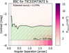 |
Fig. 3 Blended source confidence (BSC) curve from the AstraLux SDSSz image (solid black line). The colour on each angular separation and contrast bin represent the probability of a source aligned at the location of the target, based on the TRILEGAL model. The horizontal dotted line shows the maximum contrast of a blended binary that is capable of imitating the planet’s transit depth. The green region represents the regime that is not explored by the high-spatial resolution image. The BSC curve corresponds to the integration of Paligned over this region. |
3 System characterization
3.1 Parent star
From the co-added spectrum built from individual HARPSN spectra extracted with the standard DRS pipeline, we derived the following atmospheric parameters of the planet’s host star TOI-1422: effective temperature Teff, surface gravity log g, microturbulence velocity ξ, iron abundance [Fe/H], and rotational velocity v sin i⋆. For Teff, log g, ξ, and [Fe/H], we applied a method based on equivalent widths of iron lines taken from Biazzo et al. (2015) and the spectral analysis package MOOG (Sneden 1973; version 2017). The Castelli & Kurucz (2003) grid of model atmospheres was adopted. Teff and ξ were derived by imposing that the abundance of Fe I was not dependent on the line excitation potentials and the reduced equivalent widths (i.e. EW/λ), respectively, while log g was obtained by imposing the Fe I/Fe II ionization equilibrium condition. The v sin i⋆ was measured with the same MOOG code, by applying the spectral synthesis of three regions around 5400, 6200, and 6700 A, and adopting the same grid of model atmosphere after fixing the macroturbulence velocity to the value of 3.4 km s−1 from the relationship by Doyle et al. (2014). From these results, the star can be classified as a G2V dwarf with a low projected rotation velocity vsin i⋆ of 1.9 ± 0.8 km s−1, implying a maximum rotation period of  d at 1σ. Analogously, using an empirical relation based on the Full Width at Half Maximum (FWHM)9 derived by the HARPS-N DRS, we find v sin i⋆ ~ 2.2 km s−1.
The field of TOI-1422 was also observed in 2004, 2006, and 2007 during the WASP transit-search survey (Pollacco et al. 2006). A total of 20 000 photometric data points were obtained by observing the field every ~15 min on clear nights, over spans of ~ 120 days in each year. We searched the data for any rotational modulation using the methods from Maxted et al. (2011) and found no significant periodicity between 1 and 100 days, with a 95%-confidence upper limit on the amplitude of 2 mmag. The TESS light curve shows no modulation either (Sect. 2.1), confirming that the star is rather magnetically quiet over a period of ~100 days.
Moreover, the spectrum of TOI-1422 clearly shows a lithium line at λ = 6707.8 Å. We therefore estimated the lithium abundance log A(Li)NLTE by measuring the lithium EW and considering our Teff, log g, ξ, and [Fe/H] previously derived together with the NLTE corrections by Lind et al. (2009). The value of the lithium abundance is listed in Table 1 and its position in a log A(Li)-Teff diagram is compatible with the M67 open cluster advanced age (~4.5 Gyr; see Pasquini et al. 2009) in agreement with the star’s low activity level. The physical parameters of TOI-1422 are also displayed in Table 1 and were determined with the EXOFASTv2 Bayesian code (Eastman 2017; Eastman et al. 2019), by fitting the stellar spectral energy distribution (SED) and by employing the MESA Isochrones and Stellar Tracks (Dotter 2016) to more precisely constrain the stellar mass. In addition, in the table we report the stellar magnitudes used for the SED modelling, while the SED best fit is shown in Fig. 4. Gaussian priors were imposed on the Gaia eDR3 parallax (Gaia Collaboration 2021) as well as on the Teff and [Fe/H], as derived above from the analysis of the HARPS-N spectra. An upper limit was set on the V-band extinction, AV, from reddening maps (Schlegel et al. 1998; Schlafly & Finkbeiner 2011).
3.2 RV and activity indexes periodogram analysis
We computed the generalized Lomb-Scargle (GLS) periodogram for the HARPS-N RVs and different stellar activity indexes10 using the Python package astropy v.4.3.1 (Price-Whelan et al. 2018). The periodogram of the RVs shows the main peak around 29 days, and a significant peak at 13 days (TOI-1422 b transiting period), after correcting for a linear trend of ~4 m s−1 yr−1, observed in HARPS-N data. No index shows signs of the 29-day periodicity, but a linear trend is also present in the FWHM and log R′Hk (see Fig. D.1), with the former correlating the most with the RVs, unveiling a moderate Spearman coefficient (Spearman 1904) of 0.41 (p-value 0.01%). Therefore, in order to explain the nature of the main peak in the RVs, we present the GLS periodogram of these coefficients posterior to the removal of their linear trends in Fig. 5 (see Fig. D.2 for a closer look at the RVs panel), but again no trace of the 29-day signal is found. We also performed a GP regression analysis, using a quasi-periodic model, of the log R′HK index corrected for the linear trend over the time series, and find no evidence of any particular periodic modulation in the posterior distribution of the periodic time-scale hyper-parameter. In short, there is no evidence pointing to a specific periodic rotation of the star TOI-1422, other than the tentative estimation from v sin i⋆.
A query from the Gaia eDR3 archive returns astrometric excess noise and renormalized unit weight error (RUWE) values of 80 µas and 1.09, respectively, for TOI-1422. Thus, the star is astrometrically quiet. The analysis of Sect. 2.2 rules out the existence of obvious sub-arcsec stellar companions, and no co-moving objects are present in Gaia eDR3 data in a 600 arcsec radius. The linear trend seen in the RV data, along with a few activity indexes, can therefore be explained by long star magnetic activity, rather than by the presence of a companion11.
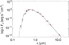 |
Fig. 4 Spectral energy distribution computed for TOI-1422, where the black curve is the most likely atmospheric stellar model and the blue dots correspond to the model fluxes over each passband. The horizontal and vertical red error bars represent, respectively, the effective width of the passbands and the reported photometric measurement uncertainties (refer to the magnitudes in Table 1). |
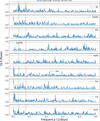 |
Fig. 5 GLS periodogram of HARPS-N RVs and of various activity indexes specified in the labels, after the removal of a linear trend (Sect. 3.2). The main peak of the RV GLS periodogram and that of the TOI-1422 b period are highlighted with a green and a red dashed line, respectively. They do not overlap with any of the peaks from the indexes, which in general do not suggest any clear stellar rotation period. The period corresponding to the highest peak in the RV GLS periodogram, and its False Alarm Probability (FAP), are written on the top of the first panel, while the horizontal dashed lines remark the 10% and 1% confidence levels (evaluated with the bootstrap method), respectively. The three peaks surrounding the RVs main frequency can all be explained as aliases of the 29-day signal due to the two highest frequencies of the window function (190 and 390.3 days, as shown in Fig. D.2 and Fig. D.3). |
3.3 RV and photometry joint analysis
A joint transit and RV analysis was carried out with juliet, which employs different Python tools: batman12 (Kreidberg 2015) for the modelling of transits, RadVel13 (Fulton et al. 2018) for the modelling of RVs, and stochastic processes, which are treated as GPs with the packages george14 (Ambikasaran et al. 2015) and celerite15. The RV model that we used in juliet is the following:
 (3)
(3)
where є(t) is a noise model for the HARPS-N instrument, here assumed to be white-Gaussian noise, in other words  , with σ(t)2 being the formal uncertainty of the RV point at time t,
  being an added jitter term, and N(µ, σ2) denoting a normal distribution with mean µ and variance σ2. K(t) is the Keplerian model of the RV star perturbations due to the orbiting planet,
  is the systemic velocity linked to the instrument, and the coefficients A, B (also referred to as RV slope and RV intercept) represent an additional linear trend used for modelling non-Keplerian signals with a period longer than the observation span. For a total number of data points N, we assumed the model likelihood to follow the likelihood of an N-dimensional multi-variate Gaussian:
![Mathematical equation: $\ln p\left( {{\bf{y}}\left| {\bf{\theta }} \right.} \right) = - {1 \over 2}\left[ {Nln2\pi + ln\left| {\rm{\Sigma }} \right| + {{\bf{r}}^T}{{\rm{\Sigma }}^{ - 1}}{\bf{r}}} \right],$](/articles/aa/full_html/2022/11/aa44079-22/aa44079-22-eq19.png) (4)
(4)
where y and θ are vectors containing, respectively, all the RV data points and instrumental parameters, while r is the residual vector given by
 (5)
(5)
The elements of the covariance matrix Σ are:
 (6)
(6)
with k equal to any GP kernel model, or zero for a pure white-noise one. In order to estimate the Bayesian posteriors and evidence, Z, of different models, we used the dynamic nested sampling package dynesty (Speagle 2020), which adaptively allocates samples based on a posterior structure and, at the same time, estimates evidence and sampling from multi-modal distributions. In general, dynamic nested sampling algorithms sample a dynamic number of live points from the prior ‘volume’ and sequentially replace the point with the lowest likelihood with a new one, while updating the Bayesian evidence by the difference ∆Z. Usually, the stopping criterion is a defined value of ∆Z, below which the algorithm is said to have converged (∆Z ≈ 0.5). However, here we used the default criterion described in Sect. 3.4 of Speagle (2020).
In order to reveal the transiting object suggested by the TESS light curve, we first ran the RV and photometry joint analysis with a simple one-planet model, using the parameters in the DVR produced by the SPOC pipeline as transit-related priors, both with a fixed null and uniformly-sampled eccentricity via the parametrization  , which is described in Eastman et al. (2013). All the priors are defined in Table B.1. In particular, we set Gaussian priors on both the limb-darkening coefficients (Claret 2017) and the star mean density ρ⋆ (Sect. 3.1), which was implemented here instead of the scaled semi-major axis, a/R⋆, because the latter can be recovered using Kepler’s third law using only the period of the respective planet, which is a direct result of any juliet run. In this way, from the single value of ρ⋆ we can evenly derive a/R⋆ in the case of multiple planets.
The best one-planet RV model fit is found with e = 0 ( ), but the scatter of the residuals is higher than the average photon-noise uncertainties for this kind of star. In fact, the same peak of 29 days, which was found in the RV GLS periodogram, is also distinctly found in the residuals of the transiting one-planet model (see Fig. 6). Consequently, we proceeded to test two-planet models, whose priors are summed in Table B.2. Since they have comparable statistical significance (
 ), we use the results of the eccentric model for the rest of the paper. The two-planet eccentric model is plotted on top of the RVs in Fig. 7, along with its residuals. TOI-1422 b RV semi-amplitude and orbital period are found to be
  m s−1 and Ph = 12.9972 ± 0.0006 days, respectively. The second planet, candidate TOI-1422 c, has an RV semi-amplitude of
  m s−1, orbital period of
  days and T0,c = 2458776.6 ± 4.6 BJD (see the posteriors in Fig. C.1 and Table B.3). The eccentricities turn out to be
  and
and  , but it is important to note that when they are fixed to zero, the orbital parameters of TOI-1422 b and TOI-1422 c remain, within 1-σ, compatible with those of the eccentric model.
TOI-1422 parameters.
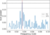 |
Fig. 6 GLS periodogram of the transiting one-planet model RV residuals. The main peak is highlighted in red and corresponds to a period of 29.2 days, with a FAP of 0.45% (evaluated with the bootstrap method), while the horizontal dashed lines show the 10% and 1% confidence levels. |
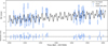 |
Fig. 7 RV measurements of TOI-1422 versus time are shown on the top panel, while their residuals over the model fit are in the bottom panel. The circles with blue error bars are the RV data taken with HARPS-N. The large and small error bars indicate σt and σw (the added jitter term), respectively. In the top panel, the black line represents the two-planet model fit. |
3.4 Results
TOI-1422 c’s orbital period explains both the main peak found in the residuals of the one-planet model (Fig. 6) and in the RV GLS periodogram (Fig. 5); it is also in 9:4 orbital resonance with the first planet. The difference between the Bayesian evidence of the two-planet eccentric model and the one-planet model ( ) is barely above the very strong evidence threshold defined in Kass & Raftery (1995) (∆ ln Z > 5), so even if the existence of candidate planet c remains unproven, we believe the two-planet model is currently the better one to explain the 29-day signal observed in the RVs, due to the lack of evidence of star activity.
Furthermore, the two-planet analysis was replicated with different numbers of data points in order to understand how and if new measurements were impacting the significance of the second planet detection. As shown in Fig. 8, both the RV semiamplitude and the period seem to stabilize after ≈60 measurements, which matches the beginning of the second observation season, while the significance of the 29-day peak also grows (Fig. D.4). It is noteworthy to mention that the GLS periodogram of the residuals of the two-planet model does not show peaks below 50% FAP, and hence does not suggest the presence of additional detectable signals.
A phase-folded plot of both the transit and the RVs is shown in Fig. 9 for the eccentric two-planet model. The radius for TOI-1422 b was calculated with the transformations provided by Espinoza (2018) and, using the stellar radius from Sect. 3.1, its revised value turns out to be  . Using the stellar radius from Table 1, we derived the mass of both objects to be
  and
and  . Their final parameters are reported in Table 2. An independent joint analysis of the HARPS-N RVs and TESS photometry, after the transits were normalized through a local linear fitting, was also performed with a DE-MCMC method (Eastman et al. 2013, 2019), following the same implementation as in Bonomo et al. (2014, 2015). The obtained results are consistent, within 1-σ, with those reported in Table 2.
In order to evaluate possible transit time variations (TTVs) due to the influence of candidate TOI-1422 c over TOI-1422 b, we plot the four mid-transit times minus their expected values (based on the two-planet eccentric model) in Fig. 10, along with different TTV predictions made with the code described in Agol & Deck (2016). Unfortunately, there are not enough transits to draw any conclusions, as all the delays are compatible with zero within 1-σ. Therefore, further precise monitoring of TOI-1422 b transits is encouraged in order to confirm the existence of TOI-1422 c and, overall, better characterize the planetary system.
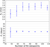 |
Fig. 8 RV semi-amplitude K and orbital period P, along with their 1-σ error bars, for candidate planet c, as functions of the number of data points used for the two-planet eccentric model analysis with juliet. |
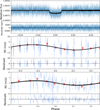 |
Fig. 9 TESS light curve and RV curves phase-folded. Top panel: TOI-1422 b transit, compared to the best-fitting model. Bottom panels: HARPS-N RV data phase-folded to the period of planet b (middle) and candidate c (bottom), along with their residuals over the model. The red circles represent the average value of phased RV data points. |
3.5 Other transit events
In the search for TOI-1422 c transits, we found a possible single transit-like event around 2 458 756.35 BTJD days, as shown in Fig. 11, which cannot be related to either TOI-1422 b or TOI-1422 c. We fitted this potential transit using the light curve from the pipeline PATHOS (Nardiello et al. 2019) and retrieved a possible radius of  , which is compatible with the transit depth observed in the PDC-SAP and SAP light curves as well. The duration of the transit suggests an orbital period longer than that for TOI-1422 c, but this is very uncertain, while the lack of other transits in the TESS light curve suggests an orbital period between 17 and 22, or longer than, 35 days, thus incompatible with that of TOI-1422 c. PATHOS is a PSF-based approach to TESS data that minimizes the dilution effects in crowded environments, and here it is utilized to extract high-precision photometry of TOI-1422 to independently confirm the presence of this transit even after the application of a different neighbour-subtraction technique. Neither the single transit nor TOI-1422 b transits show correlation with the X,Y pixels and the sky background signal (Fig. D.5), and the single transit depth also does not change with different photometric apertures (Fig. D.6). Nevertheless, the three-planet model for the joint transit-RV analysis is not statistically significant and the lack of other transits makes the suggestion of another candidate impossible to justify.
However, no transit compatible with the expected T0,c and Pc evaluated with the RV and photometry joint analysis, was found in the SPOC (both SAP and PDC-SAP) light curves, even though a small part of the supposed transiting window was missed by TESS. When we take into account both the time-span of the TESS light curve and TOI-1422 c expected (non-grazing) transit duration, the probability that such transits would have been missed can be estimated to be around 1% and 7%, with 1σ and 3σ uncertainty, respectively, on T0,c. Other than misaligned orbits, another possible explanation for the lack of TOI-1422 c transits is that despite its mass, which is greater than that of planet b, its size could be much smaller (similar to the high-density sub-Neptune, BD+20594b of Espinoza et al. 2016), as any object with a radius approximately below 2.8R⊕ might be disguised in the light curve noise (as proven by the, so far undetected and uncertain, single transit-like event). Ultimately, it remains unknown if candidate planet c is transiting or not, so further high-precision long photometric follow-up observations will be important to clear up this possibility, along with the nature of the single transit event. The new TESS observations of this target, during Sector 57, are definitely welcome as they might shed some light on both matters.
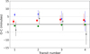 |
Fig. 10 Residuals for the mid-transit timings of TOI-1422 b versus a linear ephemeris, with 1-σ error bars, are plotted in black. The green circles, red diamonds, and blue stars represent TTV predictions in the cases of null, average, or maximum eccentricities, respectively, with the error bars showing the uncertainty due to T0,c (see Table 2). The points have been slightly shifted on the x-axis to allow for more visibility. |
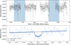 |
Fig. 11 PDC-SAP and PATHOS light curves. Top panel: TOI-1422 b transits highlighted in red in the PDC-SAP light curve, and the expected TOI-1422 c transits, with their uncertainties, highlighted in blue. A single planetary-transit event is also marked with a vertical line green, and is discussed at the end of Sect. 3.4). Bottom panel: Single transit-like event as seen in the PATHOS light curve and the corresponding fit. |
4 Discussion
4.1 Orbital resonance
As we have seen, candidate c is within in 9:4 orbital resonance with planet b. This is likely coincidental since the resonance is fifth-order, and thus very weak, unless one of the planets is quite eccentric16 or the mutual inclination is high. The exact 9:4 (or 2.25) resonance is within uncertainty, perhaps only because the uncertainty of the orbial period of TOI-1422 c is large compared to the tight period uncertainties of transiting planets. As a matter of fact, period ratios a little above two have been found within many exoplanetary systems (Winn & Fabrycky 2015), but it is also possible that the 9:4 resonance is actually the result of a resonant chain of three planets in first-order 3:2 resonances among each other, with the middle one yet to be seen. If that is the case, since the period ratios of Kepler planets near first-order resonances are usually slightly wide of resonance, the likely orbital period for this unknown exoplanet would be slightly more than 19.5 days, and thus compatible with the observed single transit discussed in Sect. 3.4. Given this orbital period and assuming that an RV semi-amplitude roughly up to 2 m s−1 might be hidden in the residuals of the two-planet model, this middle object should not have a mass higher than ≈8 M⊕, or a density higher than ≈2 g cm−3.
4.2 Mass-radius diagram and internal structure of planet b
TOI-1422 b is one of the puffier planets with a density of ~0.8 g cm−3, which is close to that of Saturn and, therefore, lower than most exoplanets in this mass range. It lies towards the upper-left corner of the mass-radius diagram (Fig. 12), making it very similar to Kepler-36c (Vissapragada et al. 2020) and especially to Kepler-11 e (Lissauer et al. 2013), which even shares the same kind of host star but is on a longer orbit. On one hand, it has a similar radius compared to Neptune and Uranus in our solar system, but on the other hand, its mass is only about 50–60% that of our ice giants. Thus, an extensive gaseous envelope, surrounding a massive core, is expected to be found in TOI-1422b. More precisely, the mass fraction of this envelope is expected to be around 10–25% of the total mass of the planet (using the equations of state from Becker et al. 2014), suggesting that the atmosphere has not been blown away by the stellar wind. The nature of this extensive envelope as well as its core requires further investigation. For this purpose, we assess the expected S/N of the JWST/NIRISS measurements17 of TOI-1422 b transits compared to planets of similar sizes, by evaluating the transmission spectroscopy metric (TSM) defined in Kempton et al. (2018):
 (7)
(7)
where the scale factor is a dimensionless normalization constant, equal to 1.28 for planets with 2.75 < R⊕ < 4.0, and J is the apparent magnitude of the host star in the J band (a filter that is near the middle of the NIRISS bandpass). As a result (Fig. 13), TOI-1422 b ranks fourth18 among Neptunes (2.75 < R⊕ < 4.0) orbiting G-F dwarfs (Teff > 5400K), but being the one with the lowest density, it is definitely an interesting candidate for atmospheric characterization by the JWST.
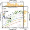 |
Fig. 12 Planetary masses and radii of the known transiting exoplanets (values taken from the Transiting Extrasolar Planet catalogueue, TEP-Cat, which is available at http://www.astro.keele.ac.uk/jkt/tepcat/catalogue; Southworth 2010, 2011) with equilibrium temperature Teq between 600 and 1000 K and host star radius between 0.6 and 1.5 R⊙. Different lines correspond to different mass fractions of relatively cold hydrogen envelopes. The ice giants of the Solar System are displayed in filled black circles. TOI-1422 b is on the low-density envelope of planets with precise mass and/or radius estimations (σMp/Mp ≤ 30%; σRp/Rp ≤ 10%), one of the reasons that make it potentially valuable for transit spectroscopy. |
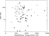 |
Fig. 13 Transmission spectroscopy observations (TSM) values with the JWST over the equilibrium temperature for planets with a measured mass in the radius range 2.75 < R⊕ < 4.0, including TOI-1422 b (green star). Filled black dots and empty squares identify the sample of planets around stars with Teff > 5400 K and Teff < 5400 K, respectively. |
5 Conclusions
In this paper, we have confirmed the planetary nature of the TESS transiting planet TOI-1422 b, which turns out to be a low-density and warm Neptune-sized planet orbiting an astrometrically, and overall magnetically, quiet G2 V star. Therefore, TOI-1422 b is the latest addition to the low-populated range of exoplanets with the size of Neptune, but with Saturn-like density. In order to well constrain the mass of TOI-1422b, a long RV monitoring with more than a hundred observations was necessary with the HARPS-N instrument at the TNG in La Palma, which resulted in fully characterized orbital and physical parameters of this new planetary system. On top of that, our RV measurements also suggest the presence in the system of a possibly non-transiting, heavier candidate planet, TOI-1422 c, in a weak 9:4 orbital resonance with its inner brother, which will require further study to validate.
Acknowledgements
We acknowledge the use of public TESS data from pipelines at the TESS Science Office and at the TESS Science Processing Operations Center. Resources supporting this work were provided by the NASA HighEnd Computing (HEC) Program through the NASA Advanced Supercomputing (NAS) Division at Ames Research Center for the production of the SPOC data products. The research has made use of the SIMBAD database, operated at CDS, Strasbourg, France, NASA’s Astrophysics Data System and the NASA Exoplanet Archive, which is operated by the California Institute of Technology, under contract with the National Aeronautics and Space Administration under the Exoplanet Exploration Program. This research was also partly supported by the Department of Energy under awards DE-NA0003904 and DE-FOA0002633 (to S.B.J., principal investigator, and collaborator Li Zeng) with Harvard University and by the Sandia Z Fundamental Science Program. This research represents the authors’ views and not those of the Department of Energy. The work is based on observations made with the Italian Telescopio Nazionale Galileo (TNG) operated on the island of La Palma by the Fundacion Galileo Galilei of the INAF (Istituto Nazionale di Astrofísica) at the Spanish Observatorio del Roque de los Muchachos of the Instituto de Astrofísica de Canarias. This work has also made use of data from the European Space Agency (ESA) mission Gaia (https://www.cosmos.esa.int/gaia), processed by the Gaia Data Processing and Analysis Consortium (DPAC, https://www.cosmos.esa.int/web/gaia/dpac/consortium). Funding for the DPAC has been provided by national institutions, in particular the institutions participating in the Gaia Multilateral Agreement. L.M. acknowledges support from the “Fondi di Ricerca Scientifica d’Ateneo 2021” of the University of Rome “Tor Vergata”. J.L-B. acknowledges financial support received from “la Caixa” Foundation (ID 100010434) and from the European Union’s Horizon 2020 research and innovation programme under the Marie Slodowska-Curie grant agreement No 847648, with fellowship code LCF/BQ/PI20/11760023. This research has also been partly funded by the Spanish State Research Agency (AEI) Projects No. PID2019-107061GB-C61 and No. MDM-2017-0737 Unidad de Excelencia “Maria de Maeztu”- Centro de Astrobiologia (INTA-CSIC). We acknowledge financial contribution from the agreement ASI-INAF no. 2018-16-HH.0. D.D. acknowledges support from the TESS Guest Investigator Program grants 80NSSC21K0108 and 80NSSC22K0185. L.N. acknowledges the support of the ARIEL ASI-INAF agreement 2021-5-HH.0.
Appendix A HARPS-N RV datapoints
Appendix B Priors and posteriors
Prior volume for the parameters of the one-planet model fit of Sect. 2.3 processed with juliet. U(a, b) indicates a uniform distribution between a and b; L(a, b) a log-normal distribution, N(a, b) a normal distribution, and T(a, b) a truncated normal distribution (where lower possible value equals zero) with mean a and standard deviation b.
Appendix C Corner plots
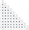 |
Fig. C.1 Corner plot for the posterior distribution of the joint transit and RV analysis of Sect. 3.3 in the case of two planets, elaborated with juliet. |
Appendix D Additional plots
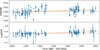 |
Fig. D.1 FWHM and log R′HK are plotted over time respectively in the upper and lower panel, along with their linear trends (orange line) and average value (dashed grey line). |
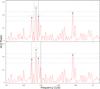 |
Fig. D.2 Close-up look of the RV GLS periodogram, executed with the publicly available tool Exo-Striker (Trifonov 2019; https://github.com/3fon3fonov/exostriker) after the removal of a linear trend. The two vertical blue lines, around the 29-day signal (indicated by a vertical yellow line), show the main peak aliases due to the two highest frequencies of the window function, in the upper and bottom panels. The three horizontal dotted lines represent the 10%, 1%, and 0.1% FAP levels. |
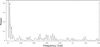 |
Fig. D.3 Window function of the HARPS-N RV measurements, as evaluated with Exo-Striker. The two highest peaks, excluding the 1-day peak and frequencies close to zero, are indicated by the respective labels. |
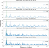 |
Fig. D.4 Unnormalized GLS power for a different number of HARPS-N observations. The power of the 29-day signal increases with more observations. The vertical dashed red and green lines indicate TOI-1422 b and TOI-1422 c orbital periods, respectively, while the horizontal dashed lines signal the 10% and 1% confidence levels, respectively (evaluated with the bootstrap method). |
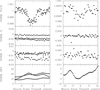 |
Fig. D.5 TOI-1422 b transits, as seen with PATHOS, folded on the first row of the left column and the single transit event on the right one, with X/Y and the sky background in the following rows, showing no correlation with the transits. |
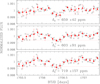 |
Fig. D.6 Single transit depth from PATHOS in different apertures, with the three rows showing the transit depth at an aperture radius of 2, 3, and 4 pixels, respectively. |
References
- Agol, E., & Deck, K. 2016, ApJ, 818, 177 [Google Scholar]
- Aller, A., Lillo-Box, J., Jones, D., Miranda, L. F., & Barceló Forteza, S. 2020, A&A, 635, A128 [NASA ADS] [CrossRef] [EDP Sciences] [Google Scholar]
- Ambikasaran, S., Foreman-Mackey, D., Greengard, L., Hogg, D. W., & O’Neil, M. 2015, IEEE Trans. Pattern Anal. Mach. Intell., 38, 252 [Google Scholar]
- Anglada-Escudé, G., & Butler, R. P. 2012, ApJS, 200, 15 [Google Scholar]
- Armstrong, D. J., Lopez, T. A., Adibekyan, V., et al. 2020, Nature, 583, 39 [Google Scholar]
- Bailer-Jones, C. A. L., Rybizki, J., Fouesneau, M., Demleitner, M., & Andrae, R. 2021, VizieR Online Data Catalog: I/352 [Google Scholar]
- Barstow, J. K., Aigrain, S., Irwin, P. G. J., Kendrew, S., & Fletcher, L. N. 2015, MNRAS, 448, 2546 [NASA ADS] [CrossRef] [Google Scholar]
- Becker, A., Lorenzen, W., Fortney, J. J., et al. 2014, ApJS, 215, 21 [NASA ADS] [CrossRef] [Google Scholar]
- Bhatti, W., Bouma, L., Joshua, John., & Price-Whelan, A. 2020, https://doi.org/10.5281/zenodo.3723832 [Google Scholar]
- Biazzo, K., Gratton, R., Desidera, S., et al. 2015, A&A, 583, A135 [NASA ADS] [CrossRef] [EDP Sciences] [Google Scholar]
- Biazzo, K., Bozza, V., Mancini, L., & Sozzetti, A. 2022, in Astrophysics and Space Science Library, Demographics of Exoplanetary Systems, Lecture Notes of the 3rd Advanced School on Exoplanetary Science, eds. K. Biazzo, V. Bozza, L. Mancini, & A. Sozzetti, 466, 143 [NASA ADS] [Google Scholar]
- Bitsch, B., Raymond, S. N., & Izidoro, A. 2019, A&A, 624, A109 [NASA ADS] [CrossRef] [EDP Sciences] [Google Scholar]
- Bonomo, A. S., Sozzetti, A., Lovis, C., et al. 2014, A&A, 572, A2 [NASA ADS] [CrossRef] [EDP Sciences] [Google Scholar]
- Bonomo, A. S., Sozzetti, A., Santerne, A., et al. 2015, A&A, 575, A85 [NASA ADS] [CrossRef] [EDP Sciences] [Google Scholar]
- Borsa, F., Allart, R., Casasayas-Barris, N., et al. 2021, A&A, 645, A24 [EDP Sciences] [Google Scholar]
- Borucki, W. J., Koch, D., Basri, G., et al. 2010, Science, 327, 977 [Google Scholar]
- Bouchy, F., Díaz, R. F., Hébrard, G., et al. 2013, A&A, 549, A49 [NASA ADS] [CrossRef] [EDP Sciences] [Google Scholar]
- Brande, J., Crossfield, I. J. M., Kreidberg, L., et al. 2022, AJ, accepted [arXiv:2201.04197] [Google Scholar]
- Brogi, M., Giacobbe, P., Guilluy, G., et al. 2018, A&A, 615, A16 [NASA ADS] [CrossRef] [EDP Sciences] [Google Scholar]
- Brown, A. G. A., Vallenari, A., Prusti, T., et al. 2018, A&A, 616, A1 [NASA ADS] [CrossRef] [EDP Sciences] [Google Scholar]
- Brown, A. G. A., Vallenari, A., Prusti, T., et al. 2021, A&A, 650, C3 [NASA ADS] [CrossRef] [EDP Sciences] [Google Scholar]
- Bryson, S. T., Jenkins, J. M., Klaus, T. C., et al. 2020, Kepler Data Processing Handbook: Target and Aperture Definitions: Selecting Pixels for Kepler Downlink, Kepler Science Document KSCI-19081-003 [Google Scholar]
- Bryson, S. T., Jenkins, J. M., Klaus, T. C., et al. 2010, SPIE Conf. Ser., 7740, 77401D [NASA ADS] [Google Scholar]
- Buchhave, L. A., Bizzarro, M., Latham, D. W., et al. 2014, Nature, 509, 593 [Google Scholar]
- Carleo, I., Desidera, S., Nardiello, D., et al. 2021, A&A, 645, A71 [EDP Sciences] [Google Scholar]
- Casasayas-Barris, N., Pallé, E., Yan, F., et al. 2019, A&A, 628, A9 [NASA ADS] [CrossRef] [EDP Sciences] [Google Scholar]
- Castelli, F., & Kurucz, R. L. 2003, in Modelling of Stellar Atmospheres, eds. N. Piskunov, W. W. Weiss, & D. F. Gray, 210, A20 [Google Scholar]
- Chontos, A., Murphy, J. M. A., MacDougall, M. G., et al. 2022, AJ, 163, 297 [NASA ADS] [CrossRef] [Google Scholar]
- Claret, A. 2017, A&A, 600, A30 [NASA ADS] [CrossRef] [EDP Sciences] [Google Scholar]
- Cloutier, R., Eastman, J. D., Rodriguez, J. E., et al. 2020, AJ, 160, 3 [Google Scholar]
- Cosentino, R., Lovis, C., Pepe, F., et al. 2012, Society of Photo-Optical Instrumentation Engineers (SPIE) Conference Series, Harps-N: the new planet hunter at TNG, 8446, 84461V [NASA ADS] [Google Scholar]
- Covino, E., Esposito, M., Barbieri, M., et al. 2013, A&A, 554, A28 [NASA ADS] [CrossRef] [EDP Sciences] [Google Scholar]
- Cumming, A., Butler, R. P., Marcy, G. W., et al. 2008, PASP, 120, 531 [CrossRef] [Google Scholar]
- Cutri, R. M., Wright, E. L., Conrow, T., et al. 2021, VizieR Online Data Catalog: II/328 [Google Scholar]
- Delrez, L., Ehrenreich, D., Alibert, Y., et al. 2021, Nat. Astron., 5, 775 [NASA ADS] [CrossRef] [Google Scholar]
- Diamond-Lowe, H., Berta-Thompson, Z., Charbonneau, D., & Kempton, E. M. R. 2018, AJ, 156, 42 [NASA ADS] [CrossRef] [Google Scholar]
- Dotter, A. 2016, ApJS, 222, 8 [Google Scholar]
- Doyle, A. P., Davies, G. R., Smalley, B., Chaplin, W. J., & Elsworth, Y. 2014, MNRAS, 444, 3592 [Google Scholar]
- Eastman, J. 2017, EXOFASTv2: Generalized publication-quality exoplanet modeling code, Astrophysics Source Code Library [record ascl:1710.003] Eastman, J., Gaudi, B. S., & Agol, E. 2013, PASP, 125, 83 [Google Scholar]
- Eastman, J. D., Rodriguez, J. E., Agol, E., et al. 2019, PASP, submitted [arXiv:1907.09480] [Google Scholar]
- Espinoza, N. 2018, RNAAS, 2, 209 [Google Scholar]
- Espinoza, N., Brahm, R., Jordán, A., et al. 2016, ApJ, 830, 43 [NASA ADS] [CrossRef] [Google Scholar]
- Espinoza, N., Kossakowski, D., & Brahm, R. 2019, MNRAS, 490, 2262 [Google Scholar]
- Foreman-Mackey, D., Agol, E., Ambikasaran, S., & Angus, R. 2017, AJ, 154, 220 [Google Scholar]
- Fressin, F., Torres, G., Charbonneau, D., et al. 2013, ApJ, 766, 81 [NASA ADS] [CrossRef] [Google Scholar]
- Fulton, B. J., & Petigura, E. A. 2018, AJ, 156, 264 [Google Scholar]
- Fulton, B. J., Petigura, E. A., Blunt, S., & Sinukoff, E. 2018, PASP, 130, 044504 [Google Scholar]
- Gaia Collaboration (Brown, A. G. A., et al.) 2021, A&A, 649, A1 [NASA ADS] [CrossRef] [EDP Sciences] [Google Scholar]
- Gandolfi, D., Barragán, O., Livingston, J. H., et al. 2018, A&A, 619, A10 [Google Scholar]
- Girardi, L., Barbieri, M., Groenewegen, M. A. T., et al. 2012, Astrophys. Space Sc. Proc., 26, 165 [NASA ADS] [CrossRef] [Google Scholar]
- Gomes da Silva, J., Figueira, P., Santos, N., & Faria, J. 2018, J. Open Source Softw., 3, 667 [Google Scholar]
- Gray, R. O., & Corbally, C. 2009, Stellar Spectral Classification (Princeton University Press) [CrossRef] [Google Scholar]
- Guerrero, N. M., Seager, S., Huang, C. X., et al. 2021, ApJS, 254, 39 [NASA ADS] [CrossRef] [Google Scholar]
- Henden, A. A., Levine, S., Terrell, D., & Welch, D. L. 2015, in American Astronomical Society Meeting Abstracts, 225, 336.16 [Google Scholar]
- Høg, E., Fabricius, C., Makarov, V. V., et al. 2000, A&A, 355, L27 [Google Scholar]
- Hormuth, F., Brandner, W., Hippler, S., & Henning, T. 2008, J. Phys. Conf. Ser., 131, 012051 [Google Scholar]
- Howard, A. W., Marcy, G. W., Johnson, J. A., et al. 2010, Science, 330, 653 [Google Scholar]
- Howard, A. W., Marcy, G. W., Bryson, S. T., et al. 2012, ApJS, 201, 15 [Google Scholar]
- Howell, S. B., Sobeck, C., Haas, M., et al. 2014, PASP, 126, 398 [Google Scholar]
- Hunter, A., Macgregor, A. B., Szabo, T., Wellington, C., & Bellgard, M. I. 2012, Source Code Biol. Med., 7, 1 [CrossRef] [Google Scholar]
- Jenkins, J. M. 2002, ApJ, 575, 493 [Google Scholar]
- Jenkins, J. M., Chandrasekaran, H., McCauliff, S. D., et al. 2010, SPIE Conf. Ser., 7740, 77400D [Google Scholar]
- Jenkins, J. M., Twicken, J. D., McCauliff, S., et al. 2016, SPIE Conf. Ser., 9913 99133E [Google Scholar]
- Jenkins, J. M., Tenenbaum, P., Seader, S., et al. 2020, Kepler Data Processing Handbook: Transiting Planet Search, ed. J. M. Jenkins. Kepler Science Document KSCI-19081-003, 9 [Google Scholar]
- Kane, S. R., Yalçınkaya, S., Osborn, H. P., et al. 2020, AJ, 160, 129 [NASA ADS] [CrossRef] [Google Scholar]
- Kass, R. E., & Raftery, A. E. 1995, J. Am. Stat. Assoc., 90, 773 [Google Scholar]
- Kempton, E. M.-R., Bean, J. L., Louie, D. R., et al. 2018, PASP, 130, 114401 [CrossRef] [Google Scholar]
- Kipping, D. M. 2013, MNRAS, 435, 2152 [Google Scholar]
- Knutson, H. A., Benneke, B., Deming, D., & Homeier, D. 2014, Nature, 505, 66 [Google Scholar]
- Kreidberg, L. 2015, PASP, 127, 1161 [Google Scholar]
- Kreidberg, L., Bean, J. L., Désert, J.-M., et al. 2014, Nature, 505, 69 [Google Scholar]
- Lacedelli, G., Malavolta, L., Borsato, L., et al. 2020, MNRAS, 501, 4148 [Google Scholar]
- Lacedelli, G., Wilson, T. G., Malavolta, L., et al. 2022, MNRAS, 511, 4551 [NASA ADS] [CrossRef] [Google Scholar]
- Li, J., Tenenbaum, P., Twicken, J. D., et al. 2019, PASP, 131, 1 [Google Scholar]
- Lightkurve Collaboration (Cardoso, J. V. D. M., et al.) 2018, Lightkurve: Kepler and TESS time series analysis in Python, Astrophysics Source Code Library [record ascl:1812.013] [Google Scholar]
- Lillo-Box, J., Barrado, D., & Bouy, H. 2012, A&A, 546, A10 [NASA ADS] [CrossRef] [EDP Sciences] [Google Scholar]
- Lillo-Box, J., Barrado, D., & Bouy, H. 2014, A&A, 566, A103 [NASA ADS] [CrossRef] [EDP Sciences] [Google Scholar]
- Lind, K., Asplund, M., & Barklem, P. S. 2009, A&A, 503, 541L [NASA ADS] [CrossRef] [EDP Sciences] [Google Scholar]
- Lissauer, J. J., Jontof-Hutter, D., Rowe, J. F., et al. 2013, ApJ, 770, 131 [Google Scholar]
- Lozovsky, M., Helled, R., Dorn, C., & Venturini, J. 2018, ApJ, 866, 49 [Google Scholar]
- Maxted, P. F. L., Anderson, D. R., Collier Cameron, A., et al. 2011, PASP, 123, 547 [NASA ADS] [CrossRef] [Google Scholar]
- Mayor, M., Marmier, M., Lovis, C., et al. 2011, ArXiv e-prints, [arXiv:1109.2497] [Google Scholar]
- Miller-Ricci, E., Seager, S., & Sasselov, D. 2009, ApJ, 690, 1056 [Google Scholar]
- Modirrousta-Galian, D., Locci, D., & Micela, G. 2020, ApJ, 891, 158 [Google Scholar]
- Morris, R. L., Twicken, J. D., Smith, J. C., et al. 2020, Kepler Data Processing Handbook: Photometric Analysis, ed. J. M. Jenkins, Kepler Science Document KSCI-19081-003, id. 6 [Google Scholar]
- Nardiello, D., Borsato, L., Piotto, G., et al. 2019, MNRAS, 490, 3806 [NASA ADS] [CrossRef] [Google Scholar]
- Pasquini, L., Biazzo, K., Bonifacio, P., Randich, S., & Bedin, L. R. 2009, A&A, 489, 677Perger, M., García-Piquer, A., Ribas, I., et al. 2017, A&A, 598, A26 [Google Scholar]
- Perruchot, S., Kohler, D., Bouchy, F., et al. 2008, in Ground-based and Airborne Instrumentation for Astronomy II, eds. I. S. McLean, & M. M. Casali, International Society for Optics and Photonics (SPIE), 7014, 235 [Google Scholar]
- Petigura, E. A., Howard, A. W., Marcy, G. W., et al. 2017, AJ, 154, 107 [NASA ADS] [CrossRef] [Google Scholar]
- Petigura, E. A., Marcy, G. W., & Howard, A. W. 2013, ApJ, 770, 69 [NASA ADS] [CrossRef] [Google Scholar]
- Pino, L., Désert, J.-M., Brogi, M., et al. 2020, ApJ, 894, L27 [Google Scholar]
- Pollacco, D. L., Skillen, I., Collier Cameron, A., et al. 2006, PASP, 118, 1407 [NASA ADS] [CrossRef] [Google Scholar]
- Poretti, E., Boccato, C., Claudi, R., et al. 2016, Mem. Soc. Astron. Italiana, 87, 141 [NASA ADS] [Google Scholar]
- Price-Whelan, A. M., Sipocz, B. M., Günther, H. M., et al. 2018, AJ, 156, 123 [NASA ADS] [CrossRef] [Google Scholar]
- Prusti, T., de Bruijne, J. H. J., Brown, A. G. A., et al. 2016, A&A, 595, A1 [NASA ADS] [CrossRef] [EDP Sciences] [Google Scholar]
- Ramsay, S., Cirasuolo, M., Amico, P., et al. 2021, The Messenger, 182, 3 [NASA ADS] [Google Scholar]
- Ricker, G. R., Winn, J. N., Vanderspek, R., et al. 2014, Proceedings of the SPIE, 9143, 914320 [NASA ADS] [CrossRef] [Google Scholar]
- Scarsdale, N., Murphy, J. M. A., Batalha, N. M., et al. 2021, AJ, 162, 215 [NASA ADS] [CrossRef] [Google Scholar]
- Schlafly, E. F., & Finkbeiner, D. P. 2011, ApJ, 737, 103 [Google Scholar]
- Schlegel, D. J., Finkbeiner, D. P., & Davis, M. 1998, ApJ, 500, 525 [Google Scholar]
- Skidmore, W., TMT International Science Development Teams, & Science Advisory Committee, T. 2015, Res. Astron. Astrophys., 15, 1945 [CrossRef] [Google Scholar]
- Skrutskie, M. F., Cutri, R. M., Stiening, R., et al. 2006, AJ, 131, 1163 [NASA ADS] [CrossRef] [Google Scholar]
- Smith, J. C., Stumpe, M. C., Cleve, J. E. V., et al. 2012, PASP, 124, 1000 [NASA ADS] [CrossRef] [Google Scholar]
- Sneden, C. 1973, AJ, 184, 839 [NASA ADS] [CrossRef] [Google Scholar]
- Snellen, I. A. G., de Kok, R. J., de Mooij, E. J. W., & Albrecht, S. 2010, Nature, 465, 1049 [Google Scholar]
- Southworth, J. 2010, MNRAS, 408, 1689 [Google Scholar]
- Southworth, J. 2011, MNRAS, 417, 2166 [Google Scholar]
- Speagle, J. S. 2020, MNRAS, 493, 3132 [Google Scholar]
- Spearman, C. 1904, Am. J. Psychol., 15, 72 [Google Scholar]
- Stassun, K. G., Oelkers, R. J., Pepper, J., et al. 2018, AJ, 156, 102 [Google Scholar]
- Stassun, K. G., Oelkers, R. J., Paegert, M., et al. 2019, AJ, 158, 138 [Google Scholar]
- Strehl, K. 1902, Astron. Nachr., 158, 89 [Google Scholar]
- Stumpe, M. C., Smith, J. C., Van Cleve, J. E., et al. 2012, PASP, 124, 985 [Google Scholar]
- Stumpe, M. C., Smith, J. C., Catanzarite, J. H., et al. 2014, PASP, 126, 100 [Google Scholar]
- Tinetti, G., Eccleston, P., Haswell, C., et al. 2021, ArXiv e-prints, [arXiv:2104.04824] [Google Scholar]
- Trifonov, T. 2019, The Exo-Striker: Transit and radial velocity interactive fitting tool for orbital analysis and N-body simulations, Astrophysics Source Code Library [record ascl:1906.004] [Google Scholar]
- Turbet, M., Bolmont, E., Ehrenreich, D., et al. 2020, A&A, 638, A41 [NASA ADS] [CrossRef] [EDP Sciences] [Google Scholar]
- Twicken, J. D., Catanzarite, J. H., Clarke, B. D., et al. 2018, PASP, 130, 064502 [Google Scholar]
- Twicken, J. D., Clarke, B. D., Bryson, S. T., et al. 2010, in Software and Cyberinfrastructure for Astronomy, eds. N. M. Radziwill, & A. Bridger, International Society for Optics and Photonics (SPIE), 7740, 749 [Google Scholar]
- Van Eylen, V., Agentoft, C., Lundkvist, M. S., et al. 2018, MNRAS, 479, 4786 [Google Scholar]
- Vissapragada, S., Jontof-Hutter, D., Shporer, A., et al. 2020, AJ, 159, 108 [NASA ADS] [CrossRef] [Google Scholar]
- Weiss, L. M., & Marcy, G. W. 2014, ApJ, 783, L6 [Google Scholar]
- Winn, J. N., & Fabrycky, D. C. 2015, ARA&A, 53, 409 [Google Scholar]
- Wright, J. T., Marcy, G. W., Howard, A. W., et al. 2012, ApJ, 753, 160 [Google Scholar]
- Wyttenbach, A., Ehrenreich, D., Lovis, C., Udry, S., & Pepe, F. 2015, A&A, 577, A62 [NASA ADS] [CrossRef] [EDP Sciences] [Google Scholar]
- Xie, J.-W., Dong, S., Zhu, Z., et al. 2016, Proc. Natl. Acad. Sci., 113, 11431 [Google Scholar]
- Zeng, L., Jacobsen, S. B., Sasselov, D. D., et al. 2019, Proc. Natl. Acad. Sci. U.S.A., 116, 9723 [Google Scholar]
For a possible explanation of Fulton’s gap, see Modirrousta-Galian et al. (2020).
tpfplotter is a python package developed by J. Lillo-Box and publicly available on www.github.com/jlillo/tpfplotter.
Since the release of the light curve products from Year 2, the SPOC background estimation algorithm has been updated due to an over-correction bias, which was significant for dim and/or crowded targets. For this particular TOI, we estimated this over-correction to be negligible for the planetary radius estimation as it is significantly smaller than the transit depth uncertainty.
This is done in python by using the astrobase implementation by Bhatti et al. (2020).
For a comparison of the performances of TERRA vs. DRS see Perger et al. (2017).
This relation was calibrated using a set of well-aligned transiting exoplanet systems, for which we could infer v sin i⋆ as equal to their equatorial velocities. We estimate the equatorial velocities from the stellar radii and rotational period, and correlated these values directly to the FWHMs.
The FWHM and the Bisector inverse span (BIS) are calculated using the cross correlation function (CCF) derived by the DRS pipeline. We also analysed the chromospheric log R′HK index, and additional activity diagnostics derived from the spectroscopic lines He I, Na I, Ca I, Hα06 and Hα16 as defined in the code ACTIN (https://github.com/gomesdasilva/ACTIN v.1.3.9, Gomes da Silva et al. 2018) which has been used for the calculation. In particular, the two H-alpha indices have 1.6 and 0.6 Å band-pass width, respectively.
In this case, at a projected separation of 0.1 arcsec (~15 au at the distance of TOI-1422), the lower limit of the AstraLux imaging data, a maximum RV slope of the magnitude measured in this work would be produced by a companion of ~30 MJup (i.e. either a very low-mass star or a massive sub-stellar companion).
We note that, even with the e’s suggested by the eccentric fits, which are unusually high compared to most multi-transiting planetary systems according to Xie et al. (2016), the 9:4 would not be as strong as a firstorder resonance.
From a 10-h observing programme assuming a cloud-free, solar-metallicity, H2-dominated atmosphere.
Following TOI-561c (Lacedelli et al. 2020, 2022), HD 136352 c (Kane et al. 2020; Delrez et al. 2021) and HD 63935 b (Scarsdale et al. 2021)
All Tables
Prior volume for the parameters of the one-planet model fit of Sect. 2.3 processed with juliet. U(a, b) indicates a uniform distribution between a and b; L(a, b) a log-normal distribution, N(a, b) a normal distribution, and T(a, b) a truncated normal distribution (where lower possible value equals zero) with mean a and standard deviation b.
All Figures
|
Fig. 1 Target pixel file from the TESS observation of Sector 16, made with tpfplotter (Aller et al. 2020) and centred on TOI-1422, which is marked with a white cross. The SPOC pipeline aperture is shown by shaded red squares, and the Gaia satellite eDR3 catalogue (Brown et al. 2018; Prusti et al. 2016) is also overlaid with symbol sizes proportional to the magnitude difference with TOI-1422. The difference image centroid locates the source of the transits within 1.89 ± 5 arcsec of the target star’s location, as reported by the TicOffset for the multi-sector DV report for this system. |
| In the text | |
|
Fig. 2 Light curve of TOI-1422 as collected by TESS in Sectors 16 and 17 with a 2-min cadence. Top panel: light curve from the PDC-SAP pipeline. The black line represents the best-fit model obtained through GP detrending, as detailed in Sect. 2.1. Bottom panel: residuals of the best-fit model in parts per million. |
| In the text | |
|
Fig. 3 Blended source confidence (BSC) curve from the AstraLux SDSSz image (solid black line). The colour on each angular separation and contrast bin represent the probability of a source aligned at the location of the target, based on the TRILEGAL model. The horizontal dotted line shows the maximum contrast of a blended binary that is capable of imitating the planet’s transit depth. The green region represents the regime that is not explored by the high-spatial resolution image. The BSC curve corresponds to the integration of Paligned over this region. |
| In the text | |
|
Fig. 4 Spectral energy distribution computed for TOI-1422, where the black curve is the most likely atmospheric stellar model and the blue dots correspond to the model fluxes over each passband. The horizontal and vertical red error bars represent, respectively, the effective width of the passbands and the reported photometric measurement uncertainties (refer to the magnitudes in Table 1). |
| In the text | |
|
Fig. 5 GLS periodogram of HARPS-N RVs and of various activity indexes specified in the labels, after the removal of a linear trend (Sect. 3.2). The main peak of the RV GLS periodogram and that of the TOI-1422 b period are highlighted with a green and a red dashed line, respectively. They do not overlap with any of the peaks from the indexes, which in general do not suggest any clear stellar rotation period. The period corresponding to the highest peak in the RV GLS periodogram, and its False Alarm Probability (FAP), are written on the top of the first panel, while the horizontal dashed lines remark the 10% and 1% confidence levels (evaluated with the bootstrap method), respectively. The three peaks surrounding the RVs main frequency can all be explained as aliases of the 29-day signal due to the two highest frequencies of the window function (190 and 390.3 days, as shown in Fig. D.2 and Fig. D.3). |
| In the text | |
|
Fig. 6 GLS periodogram of the transiting one-planet model RV residuals. The main peak is highlighted in red and corresponds to a period of 29.2 days, with a FAP of 0.45% (evaluated with the bootstrap method), while the horizontal dashed lines show the 10% and 1% confidence levels. |
| In the text | |
|
Fig. 7 RV measurements of TOI-1422 versus time are shown on the top panel, while their residuals over the model fit are in the bottom panel. The circles with blue error bars are the RV data taken with HARPS-N. The large and small error bars indicate σt and σw (the added jitter term), respectively. In the top panel, the black line represents the two-planet model fit. |
| In the text | |
|
Fig. 8 RV semi-amplitude K and orbital period P, along with their 1-σ error bars, for candidate planet c, as functions of the number of data points used for the two-planet eccentric model analysis with juliet. |
| In the text | |
|
Fig. 9 TESS light curve and RV curves phase-folded. Top panel: TOI-1422 b transit, compared to the best-fitting model. Bottom panels: HARPS-N RV data phase-folded to the period of planet b (middle) and candidate c (bottom), along with their residuals over the model. The red circles represent the average value of phased RV data points. |
| In the text | |
|
Fig. 10 Residuals for the mid-transit timings of TOI-1422 b versus a linear ephemeris, with 1-σ error bars, are plotted in black. The green circles, red diamonds, and blue stars represent TTV predictions in the cases of null, average, or maximum eccentricities, respectively, with the error bars showing the uncertainty due to T0,c (see Table 2). The points have been slightly shifted on the x-axis to allow for more visibility. |
| In the text | |
|
Fig. 11 PDC-SAP and PATHOS light curves. Top panel: TOI-1422 b transits highlighted in red in the PDC-SAP light curve, and the expected TOI-1422 c transits, with their uncertainties, highlighted in blue. A single planetary-transit event is also marked with a vertical line green, and is discussed at the end of Sect. 3.4). Bottom panel: Single transit-like event as seen in the PATHOS light curve and the corresponding fit. |
| In the text | |
|
Fig. 12 Planetary masses and radii of the known transiting exoplanets (values taken from the Transiting Extrasolar Planet catalogueue, TEP-Cat, which is available at http://www.astro.keele.ac.uk/jkt/tepcat/catalogue; Southworth 2010, 2011) with equilibrium temperature Teq between 600 and 1000 K and host star radius between 0.6 and 1.5 R⊙. Different lines correspond to different mass fractions of relatively cold hydrogen envelopes. The ice giants of the Solar System are displayed in filled black circles. TOI-1422 b is on the low-density envelope of planets with precise mass and/or radius estimations (σMp/Mp ≤ 30%; σRp/Rp ≤ 10%), one of the reasons that make it potentially valuable for transit spectroscopy. |
| In the text | |
|
Fig. 13 Transmission spectroscopy observations (TSM) values with the JWST over the equilibrium temperature for planets with a measured mass in the radius range 2.75 < R⊕ < 4.0, including TOI-1422 b (green star). Filled black dots and empty squares identify the sample of planets around stars with Teff > 5400 K and Teff < 5400 K, respectively. |
| In the text | |
|
Fig. C.1 Corner plot for the posterior distribution of the joint transit and RV analysis of Sect. 3.3 in the case of two planets, elaborated with juliet. |
| In the text | |
|
Fig. D.1 FWHM and log R′HK are plotted over time respectively in the upper and lower panel, along with their linear trends (orange line) and average value (dashed grey line). |
| In the text | |
|
Fig. D.2 Close-up look of the RV GLS periodogram, executed with the publicly available tool Exo-Striker (Trifonov 2019; https://github.com/3fon3fonov/exostriker) after the removal of a linear trend. The two vertical blue lines, around the 29-day signal (indicated by a vertical yellow line), show the main peak aliases due to the two highest frequencies of the window function, in the upper and bottom panels. The three horizontal dotted lines represent the 10%, 1%, and 0.1% FAP levels. |
| In the text | |
|
Fig. D.3 Window function of the HARPS-N RV measurements, as evaluated with Exo-Striker. The two highest peaks, excluding the 1-day peak and frequencies close to zero, are indicated by the respective labels. |
| In the text | |
|
Fig. D.4 Unnormalized GLS power for a different number of HARPS-N observations. The power of the 29-day signal increases with more observations. The vertical dashed red and green lines indicate TOI-1422 b and TOI-1422 c orbital periods, respectively, while the horizontal dashed lines signal the 10% and 1% confidence levels, respectively (evaluated with the bootstrap method). |
| In the text | |
|
Fig. D.5 TOI-1422 b transits, as seen with PATHOS, folded on the first row of the left column and the single transit event on the right one, with X/Y and the sky background in the following rows, showing no correlation with the transits. |
| In the text | |
|
Fig. D.6 Single transit depth from PATHOS in different apertures, with the three rows showing the transit depth at an aperture radius of 2, 3, and 4 pixels, respectively. |
| In the text | |
Current usage metrics show cumulative count of Article Views (full-text article views including HTML views, PDF and ePub downloads, according to the available data) and Abstracts Views on Vision4Press platform.
Data correspond to usage on the plateform after 2015. The current usage metrics is available 48-96 hours after online publication and is updated daily on week days.
Initial download of the metrics may take a while.