| Issue |
A&A
Volume 667, November 2022
|
|
|---|---|---|
| Article Number | A11 | |
| Number of page(s) | 26 | |
| Section | Extragalactic astronomy | |
| DOI | https://doi.org/10.1051/0004-6361/202243856 | |
| Published online | 28 October 2022 | |
Revisiting stellar properties of star-forming galaxies with stellar and nebular spectral modelling
1
Instituto de Astrofísica e Ciências do Espaço, Universidade do Porto, CAUP, Rua das Estrelas, 4150-762 Porto, Portugal
e-mail: This email address is being protected from spambots. You need JavaScript enabled to view it.
2
Instituto de Astrofísica e Ciências do Espaço, Universidade de Lisboa, OAL, Tapada da Ajuda, 1349-018 Lisboa, Portugal
3
Departamento de Física, Faculdade de Ciências da Universidade de Lisboa, Edifício C8, Campo Grande, 1749-016 Lisboa, Portugal
Received:
25
April
2022
Accepted:
22
August
2022
Abstract
Context. Spectral synthesis is a powerful tool for interpreting the physical properties of galaxies by decomposing their spectral energy distributions (SEDs) into the main luminosity contributors (e.g. stellar populations of distinct age and metallicity or ionised gas). However, the impact nebular emission has on the inferred properties of star-forming (SF) galaxies has been largely overlooked over the years, with unknown ramifications to the current understanding of galaxy evolution.
Aims. The objective of this work is to estimate the relations between stellar properties (e.g. total mass, mean age, and mean metallicity) of SF galaxies by simultaneously fitting the stellar and nebular continua and comparing them to the results derived through the more common purely stellar spectral synthesis approach.
Methods. The main galaxy sample from SDSS DR7 was analysed with two distinct population synthesis codes: FADO, which estimates self-consistently both the stellar and nebular contributions to the SED, and the original version of STARLIGHT, as representative of purely stellar population synthesis codes.
Results. Differences between codes regarding average mass, mean age and mean metallicity values can go as high as ∼0.06 dex for the overall population of galaxies and ∼0.12 dex for SF galaxies (galaxies with EW(Hα) > 3 Å), with the most prominent difference between both codes in the two populations being in the light-weighted mean stellar age. FADO presents a broader range of mean stellar ages and metallicities for SF galaxies than STARLIGHT, with the latter code preferring metallicity solutions around the solar value (Z⊙ = 0.02). A closer look into the average light- and mass-weighted star formation histories of intensively SF galaxies (EW(Hα) > 75 Å) reveals that the light contributions of simple stellar populations (SSPs) younger than ≤107 (109) years in STARLIGHT are higher by ∼5.41% (9.11%) compared to FADO. Moreover, FADO presents higher light contributions from SSPs with metallicity ≤Z⊙/200 (Z⊙/50) of around 8.05% (13.51%) when compared with STARLIGHT. This suggests that STARLIGHT is underestimating the average light-weighted age of intensively SF galaxies by up to ∼0.17 dex and overestimating the light-weighted metallicity by up to ∼0.13 dex compared to FADO (or vice versa). The comparison between the average stellar properties of passive, SF and intensively SF galaxy samples also reveals that differences between codes increase with increasing EW(Hα) and decreasing total stellar mass. Moreover, comparing SF results from FADO in a purely stellar mode with the previous results qualitatively suggests that differences between codes are primarily due to mathematical and statistical differences and secondarily due to the impact of the nebular continuum modelling approach (or lack thereof). However, it is challenging to adequately quantify the relative role of each factor since they are likely interconnected.
Conclusions. This work finds indirect evidence that a purely stellar population synthesis approach negatively impacts the inferred stellar properties (e.g. mean age and mean metallicity) of galaxies with relatively high star formation rates (e.g. dwarf spirals, ‘green peas’, and starburst galaxies). In turn, this can bias interpretations of fundamental relations such as the mass-age or mass-metallicity, which are factors worth bearing in mind in light of future high-resolution spectroscopic surveys at higher redshifts (e.g. MOONS and 4MOST-4HS).
Key words: galaxies: evolution / galaxies: starburst / galaxies: ISM / galaxies: fundamental parameters / galaxies: stellar content / methods: numerical
© L. S. M. Cardoso et al. 2022
 Open Access article, published by EDP Sciences, under the terms of the Creative Commons Attribution License (https://creativecommons.org/licenses/by/4.0), which permits unrestricted use, distribution, and reproduction in any medium, provided the original work is properly cited.
This article is published in open access under the Subscribe-to-Open model. This email address is being protected from spambots. You need JavaScript enabled to view it. to support open access publication.
1. Introduction
Understanding the complex physical processes behind Galaxy formation and evolution can be a daunting endeavour, especially with the increasing technical difficulties when looking further back in time. However, several keystone results have been obtained over the past decades: (a) high-mass galaxies assemble most of their stellar content early in their lives, whereas low-mass galaxies display relatively high specific star-formation rates (sSFRs) at a late cosmic epoch (e.g. Brinchmann et al. 2004; Noeske et al. 2007), a phenomenon known as galaxy downsizing (e.g. Cowie et al. 1995; Heavens et al. 2004; Cimatti et al. 2006), (b) there is a relative tight correlation between the stellar mass and gas-phase metallicity (e.g. Lequeux et al. 1979; Tremonti et al. 2004), (c) galaxies display a bimodal distribution based on their colour, in which they can either be large, concentrated, red and quiescent or small, less concentrated, blue and presenting signs of recent star formation (e.g. Gladders & Yee 2000; Strateva et al. 2001; Blanton et al. 2003; Kauffmann et al. 2003a; Baldry et al. 2004; Mateus et al. 2006), and (d) the seemingly linear correlation between the stellar mass and SFR in star-forming (SF) galaxies, an observable that is usually referred to as the SF main sequence of galaxies (e.g. Brinchmann et al. 2004; Noeske et al. 2007).
Notwithstanding these insights, the overall picture of galaxy formation and evolution is far from complete. For instance, a persistent issue in interpreting the physical characteristics of SF galaxies from spectral synthesis has been the relative contribution of nebular emission and its potential impact on the estimated stellar and overall galaxy properties. Indeed, several studies have shown that nebular emission (continuum and lines) can account up to ∼60% of the monochromatic luminosity at ∼5000 Å in AGN and starburst galaxies (e.g. Krüger et al. 1995; Papaderos et al. 1998; Zackrisson et al. 2001, 2008; Schaerer & de Barros 2009; Papaderos & Östlin 2012) and in optical broadband photometry, specially at low metallicities (Anders & Fritze-v. Alvensleben 2003).
For instance, Krüger et al. (1995) noted that strong star-formation activity can lead nebular continuum to contribute ∼30−70% to the total optical and near-infrared emission, whereas emission lines alone account for up to ∼45% in optical broadband photometry. From a different perspective, Reines et al. (2010) carried out spectral modelling of two young massive star clusters in NGC 4449 and showed that both the nebular continuum and line emission have a major impact on the estimated magnitudes and colours of young clusters (≲5 Myr), thus also affecting their age, mass and extinction estimates. Moreover, Izotov et al. (2011) studied a sample of 803 SF luminous compact galaxies (i.e. ‘green peas’) from the SDSS (York et al. 2000) and warned that a purely stellar spectral modelling of such objects can lead to the overestimation of the relative contribution of old stellar populations by as much as a factor of four. As the authors noted, there are two reasons for this overestimation: (a) nebular continuum increases the galaxy luminosity and (b) the nebular continuum is flatter than the stellar, thus making the overall continuum redder that it would be if it were purely stellar. Papaderos & Östlin (2012) also showed that nebular emission can introduce strong photometric biases of 0.4−1 mag in galaxies with high specific SFRs, whereas Pacifici et al. (2015) found that that SFRs can be overestimated by up ∼0.12 dex if nebular emission is neglected in spectral modelling.
The impact of these biases on the stellar mass and gas-phase metallicity relation (e.g. Tremonti et al. 2004), SF main sequence (e.g. Brinchmann et al. 2004; Noeske et al. 2007) or other scaling relations involving stellar properties is still largely unexplored. In fact, it is important to note that most spectral modelling of large-scale surveys using population synthesis has been carried assuming a purely stellar modelling approach, regardless of wether it is applied to passive, SF or even active galaxies (e.g. Kauffmann et al. 2003b; Panter et al. 2003; Cid Fernandes et al. 2005; Asari et al. 2007; Tojeiro et al. 2009; Zhong et al. 2010; Torres-Papaqui et al. 2012; Pérez et al. 2013; Sánchez-Blázquez et al. 2014; López Fernández et al. 2016; Rosa et al. 2018; Kuźmicz et al. 2019; Cai et al. 2020, 2021).
Although nebular continuum and line emission has been adopted in several evolutionary synthesis models (e.g. Leitherer et al. 1999; Schaerer 2002; Mollá et al. 2009; Martín-Manjón et al. 2010), no consistent nebular prescription has been implemented in inversion population synthesis codes until recently. Indeed, Gomes & Papaderos (2017, 2018) presented in FADO the first population synthesis code to fit self-consistently both the stellar and nebular spectral components while adopting a genetic optimisation framework. Tests revealed that this code estimates the main stellar population properties of SF galaxies (e.g. mass, mean age, and mean metallicity) within an accuracy of ∼0.2 dex (Gomes & Papaderos 2017, 2018; Cardoso et al. 2019; Pappalardo et al. 2021). For comparison, the typical level of deviations between input and inferred stellar properties when applying purely stellar population synthesis codes to evolved stellar populations with faint or absent nebular emission is of ∼0.15−0.2 dex (e.g. Cid Fernandes et al. 2005, 2014; Ocvirk et al. 2006a,b; Tojeiro et al. 2007, 2009; Koleva et al. 2009).
Moreover, Cardoso et al. (2019, hereafter CGP19) compared FADO with a purely stellar population synthesis code using synthetic galaxy models for different star formation histories (SFHs; e.g. instantaneous burst, continuous, and exponentially declining) and different fitting configurations (e.g. with or without emission lines and including or excluding the Balmer and Paschen continuum discontinuities at 3646 and 8207 Å, respectively). This work showed that applying the public version of the purely stellar population synthesis code STARLIGHT1 (Cid Fernandes et al. 2005) to spectra with a relatively high nebular continuum can lead to the overestimation of the total stellar mass by as much as ∼2 dex and the mass-weighted mean stellar age up to ∼4 dex, whereas the mean metallicity and light-weighted mean stellar age can both be underestimated by up to ∼0.6 dex. Moreover, it was found that these stellar properties can still be recovered with FADO within ∼0.2 dex in evolutionary stages with severe nebular contamination. Pappalardo et al. (2021, hereafter P21) continued this line of inquiry by adding the non-parametric purely stellar STECKMAP (Ocvirk et al. 2006a,b) to the code comparison while also exploring the impact of varying spectral quality on the derived physical properties, finding similar results and trends. It is important to note that (a) these tests were carried out using the same evolutionary models (Bruzual & Charlot 2003) both in the creation of the synthetic spectra and in the spectral modelling and (b) the input synthetic composite stellar populations were built having a constant solar metallicity (Z⊙ = 0.02). Thus, these uncertainties should be viewed as upper limits and might not necessarily directly translate into biases affecting observations.
Also recently, Gunawardhana et al. (2020) studied the stellar and nebular characteristics of massive stellar populations in the Antennae galaxy using an updated version of PLATEFIT (Tremonti et al. 2004; Brinchmann et al. 2004), capable of self-consistent modelling of the stellar and nebular continua. Spectral fitting provides estimates of the stellar and gas metallicities, stellar ages and electron temperature Te and density ne by taking as reference model libraries of HII regions built using the evolutionary synthesis code STARBURST99 (Leitherer et al. 1999) and the photoionisation code CLOUDY (Ferland et al. 1998, 2013). This work found the stellar and gas metallicity of the starbursts to be near solar and that the metallicity of the star-forming gas in the loop of NGC 4038 appears to be slightly richer than the rest of the galaxy.
Using a different approach, López Fernández et al. (2016) presented a new version of the population synthesis code STARLIGHT (Cid Fernandes et al. 2005) that combines optical spectroscopy with UV photometry. This work used a mixture of simulated and real CALIFA data (Sánchez et al. 2012) and found that the additional UV constraints have a low impact on the inferred stellar mass and dust optical depth. Although the mean age and metallicity of most galaxies remains unaffected by the additional UV spectral information, this work also showed that stellar populations of low-mass late-type galaxies are older and less chemically enriched than in purely-optical modelling. Werle et al. (2019) pursued further this line of inquiry by combining GALEX photometry with SDSS spectroscopy and found that the UV constraints lead to the increase of simple stellar populations (SSPs) with ages between ∼107 and 108 years in detriment to the relative contribution of younger and older populations, leading to slightly older mean stellar ages when weighted my mass. This redistribution of the SFH is particularly noticeable in galaxies in the low-mass end of the blue cloud. Later, Werle et al. (2020) adopted a similar approach to study early-type galaxies in the same sample and found that the UV constraints broadens the attenuation, mean stellar age and metallicity distributions. Moreover, galaxies with young stellar populations have larger Hα equivalent widths (EWs) and larger attenuations, with the metallicity of these populations being increasingly lower for larger stellar masses. Although these three works successfully use UV spectral information to constrain the contribution of young stellar populations, one wonders if the nebular continuum in galaxies with relatively high specific SFRs still needs to be accounted for as intermediate-to-old stellar populations in purely stellar spectral synthesis, in which case the lack of nebular continuum treatment would still affect the inferred stellar properties.
Taking all these factors into consideration, it is possible that the current understanding of galaxy evolution, specifically that of SF galaxies in the local universe based on large-scale survey analysis, has been affected by a lack of an adequate nebular modelling prescription in previous spectral synthesis codes. To address this subject, this work aims to revisit the relation between key stellar properties (e.g. mass, mean age, and mean metallicity) of SF galaxies by comparing the results obtained with FADO and a representative of purely stellar population synthesis codes (i.e. STARLIGHT) when applied to a well-studied large-scale survey such as SDSS (York et al. 2000).
This paper is organised as follows. Section 2 details the methodology adopted to extract and analyse the SDSS DR7 spectra using spectral synthesis. The main results of this work are presented in Sect. 3, which is particularly focussed on the relation between the main stellar properties of SF galaxies when adopting two different spectral modelling approaches. Finally, in Sects. 4–5 the findings of this work are discussed and summarised, respectively. Unless stated otherwise, this work assumes H0 = 70 km s−1 Mpc−1, ΩM = 0.3 and ΩΛ = 0.7.
2. Methodology
The population synthesis codes FADO and STARLIGHT were applied to the galaxy sample from SDSS Data Release 7 (Abazajian et al. 2009). This data set contains multi-band spectrophotometric data for 926246 objects, each with a single-fibre integrated spectrum with the wavelength range of 3800−9200 Å at a resolution of R ∼ 1800 − 2200, with the fibre covering ∼5.5 kpc of the central region of an object at z ∼ 0.1. There are several reasons to utilise this dataset: (a) photometric completeness, (b) relatively wide redshift coverage (0.02 ≲ z ≲ 0.6), (c) uniform spectral calibration, and (d) wide-range of topics related to galaxy formation and evolution that have been tackled with this data (e.g. mass–metallicity relation, Tremonti et al. 2004; stellar mass assembly, Kauffmann et al. 2003b; galaxy bimodality, Strateva et al. 2001; Blanton et al. 2003; Kauffmann et al. 2003a; Baldry et al. 2004; host-AGN relation, Kauffmann et al. 2003c; Hao et al. 2005; environmental effects on the colour-magnitude relation Hogg et al. 2004; Cooper et al. 2010).
The raw spectra were corrected for extinction using the colour excess correction factor E(B − V) computed based on the Schlegel et al. (1998) dust maps, considering the objects sky position using the right ascension and declination provided by the survey, combined with the correcting factor to E(B − V) of Schlafly & Finkbeiner (2011). The full correction equation reads,
 (1)
(1)
where  and
and  are the corrected and raw fluxes as a function of wavelength λ, respectively, and AV is the extinction in the V-band. The adopted extinction curve (also known as the reddening law) was Cardelli et al. (1989), with RV = 3.1. The spectra were then converted to the observer restframe and rebinned so that Δλ = 1 Å.
As detailed in Gomes & Papaderos (2017), the main task of the population synthesis code FADO is to reproduce the observed spectral energy distribution (SED) through a linear combination of spectral components (e.g. individual stellar spectra or SSPs) as expressed by:
 (2)
(2)
where Fλ is the flux of the observed spectrum, N⋆ is the number of unique spectral components in the adopted base library, Mi, λ0 is the stellar mass of the ith spectral component at the normalisation wavelength λ0, Lj, λ is the luminosity contribution of the ith spectral component, AV is the V-band extinction, qλ is the ratio of Aλ over AV, S(v⋆, σ⋆) denotes a Guassian kernel simulating the effect of stellar kinematics on the spectrum, with v⋆ and σ⋆ representing the stellar shift and dispersion velocities, respectively, Γλ(ne, Te) is the nebular continuum computed assuming that all stellar photons with λ ≤ 911.76 Å are absorbed and reprocessed into nebular emission, under the supposition that case B recombination applies,  is the nebular V-band extinction, and N(vη, ση) denotes the nebular kinematics kernel, with vη and ση representing the nebular shift and dispersion velocities, respectively.
It is important to note that all publicly available population synthesis codes before FADO aimed to reconstruct the observed continuum using only the first term on the right-hand side of Eq. (2), meaning, using a purely stellar scheme to reconstruct the overall observed SED (more details in Gomes & Papaderos 2017, 2018). Indeed, one of the innovative features of FADO is the inclusion of the second term, which represents the relative spectral contribution of the nebular continuum inferred from the Lyman continuum production rate of the young stellar component and scaling with the intensity of prominent Balmer lines. This makes FADO a tool specially designed to self-consistently model the stellar and nebular continuum components of SF and starburst galaxies.
Subsequently spectral fitting was carried out with both FADO2 and STARLIGHT3 between 3400 and 8900 Å using a base library with 150 SSPs from Bruzual & Charlot (2003) with a Chabrier (2003) IMF and Padova 1994 evolutionary tracks (Alongi et al. 1993; Bressan et al. 1993; Fagotto et al. 1994a,b; Girardi et al. 1996). This stellar library contains 25 ages (between 1 Myr and 15 Gyr) and six metallicities (Z = 0.0001; 0.0004; 0.004; 0.008; 0.02; 0.05 = Z⊙ × {1/200; 1/50; 1/5; 2/5; 1; 2.5}) and corresponds to an expanded version of the base adopted in CGP19, with the addition of Z⊙/200 and Z⊙/50 at the lower end of the metallicity range. The spectra were modelled assuming a Calzetti et al. (2000) extinction law, which was originally constructed taking into consideration integrated observations of SF galaxies. Moreover, the V-band extinction, stellar velocity shift and dispersion free parameters where allowed to vary in both codes within the ranges of AV = 0 − 4 mag, v⋆ = −500 − 500 km s−1 and σ⋆ = 0 − 500 km s−1, respectively. Identical parameter ranges for the velocity shift and dispersion were adopted for the nebular component in the FADO runs. Moreover, two complete runs of the whole sample were performed with STARLIGHT while changing the initial guesses in the parameter space in order to evaluate the formal errors (e.g. Ribeiro et al. 2016; Cardoso et al. 2016, 2017, 2019).
Moreover, a pre-fitting analysis was carried out with STARLIGHT using a smaller base library with 45 SSPs for 15 ages (between 1 Myr and 13 Gyr) and three metallicities (Z = {0.004; 0.02; 0.05}=Z⊙ × {1/5; 1; 2.5}) that comes with the distribution package of STARLIGHT (cf. Cid Fernandes et al. 2005). The results of this preliminary step were used to create individual spectral masks in order to exclude the most prominent emission lines in the main fitting. This was achieved by subtracting the continuum of the best-fit model from the observation and, from the resulting residual spectrum, by fitting Gaussians to the lines. The masking of these spectral regions ensures that the STARLIGHT results are more robust when it comes to SF galaxies, a procedure similar to that adopted by Asari et al. (2007) and Ribeiro et al. (2016). At the same time, FADO performs the masking of the most prominent emission lines as part of one of its built-in pre-fitting routines, as detailed in Gomes & Papaderos (2017). Three additional spectral regions are masked in both codes which are associated with small bugs in the adopted evolutionary models: 6845–6945, 7165–7210 and 7550–7725 Å (cf. Bruzual & Charlot 2003 for more details).
In addition to masking, spectral modelling was carried out while taking into consideration several spectral flags provided by the SDSS survey that are included in the mask array of each ‘fit’ file. These flags mark spectral regions with a wide range of potential problems (e.g. no observation, poor calibration, bad pixel, or sky lines) and, therefore, must be excluded from spectral synthesis. The following individual flags provided by the survey were adopted in this work: ‘Bad pixel within 3 pixels of trace’, ‘Pixel fully rejected in extraction’, ‘Sky level > flux + 10*(flux error)’, and ‘Emission line detected here’ (with the later being adopted only for STARLIGHT, for reasons previously mentioned). Choosing which individual flags to include when every pixel is important in a pixel-by-pixel code becomes an exercise in compromise. On the one hand, masking spectral regions affected by bad pixels or sky noise leads to more accurate estimates of the physical properties inferred through spectral synthesis. On the other hand, using all spectral flags computed by an automatic pipeline in any large-scale survey can lead to severe over-flagging and, thus, the removal of important spectral features. The chosen flags reflect this balancing act.
Figure 1 shows an example of spectral fits from both codes for the object ‘52912-1424-151’, a particularly noisy spectrum with S/N(λ0) = 4.4. Black, red, and blue lines on the main panel represent the input, STARLIGHT and FADO best-fit spectra, respectively. The right-hand side panels illustrate the best-fit SFHs based on the luminosity contribution L4020 of the selected SSPs at the normalisation wavelength λ0 = 4020 Å (top panels) and on their corresponding mass contributions (bottom panels). Although the mass distributions obtained with both codes differ very little, with most mass coming from SSPs older than 1 Gyr, STARLIGHT best-fit solution includes more SSPs younger than 10 Myr compared to FADO when it comes to the light distribution. Given the relatively noisy nature of the observation, this type of variations are not necessarily indicative of a strong divergence between the codes. More reliable trends are found when grouping galaxies in populations with similar spectral characteristics, as explored in Sects. 3–4.
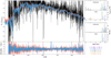 |
Fig. 1. Spectral modelling results for the SDSS DR7 spectrum ‘52912-1424-151’ using the spectral synthesis codes FADO and STARLIGHT. Main panel: black, blue and red lines represent the galaxy input spectrum and the best-fit solutions from FADO and STARLIGHT, respectively. Bottom panel: blue and red lines represent the residual spectra of FADO and STARLIGHT, respectively, that result from subtracting the best-fit solutions from the input spectrum. Top right-hand side panels: light fractions L4020 Å at the normalisation wavelength λ0 = 4020 Å as a function of the age of the SSPs in the best-fit solution of STARLIGHT (top) and FADO (bottom), with colour coding representing metallicity. Bottom right-hand side panels: mass fractions of the SSPs fitted by STARLIGHT (top) and FADO (bottom). The black vertical ticks on the top of the x-axes represent the age coverage of the adopted stellar library. |
3. Results
The following analysis is a comparison between the results from FADO and STARLIGHT, particularly regarding the stellar properties of SF galaxies (e.g. mass, mean age, and mean metallicity). Although these results could be compared to the vast number of previous works that analysed the SDSS (e.g. Brinchmann et al. 2004; Cid Fernandes et al. 2005; Tojeiro et al. 2009), this endeavour is outside of the scope of this work for several reasons.
For one, this work is a continuation of CGP19 and P21, in that it follows similar methodologies specifically interested in looking into how (not) modelling the nebular continuum in SF galaxies can impact their inferred physical properties. Moreover, it is notably difficult to ascertain the specific details regarding how previous works dealt with spectral extraction and modelling (e.g. dust treatment, spectral masking, and evolutionary ingredients). This obstacle makes direct comparisons difficult and potentially misleading, since no clear route is available to quantify the assumptions behind the different methodologies.
Last but not least, there is also the issue of aperture effects and corrections. Several works have issued cautionary remarks when attempting to apply photometric-based aperture corrections to physical properties inferred through spectral synthesis (e.g. Richards et al. 2016; Gomes et al. 2016a,b; Green et al. 2017), whilst others claim that aperture-free properties such as SFR can still be inferred (e.g. Duarte Puertas et al. 2017). Since the main objective is to compare results between two different modelling approaches, no aperture corrections are necessary. Therefore, the following discussion focus only on the galaxy surface area covered by the spectroscopic fibre.
3.1. Sample selection
The analysis of the results is based on four main samples of galaxies. The main sample (MS) is defined by a cut in apparent magnitude in the r-band of 14.5 ≤ mr ≤ 17.77 and in redshift of 0.04 ≤ z ≤ 0.4. The first criterion takes into consideration photometric completeness of the survey, whereas the second aims to remove low-redshift interlopers while also assuring that the most prominent optical emission lines (e.g. Hβλ4861; [OIII]λ5007; [OI]λ6300; Hαλ6563; [NII]λ6583; [SII]λλ6717,6731) fall within the observed wavelength range. Duplicates where removed by selecting objects classified as galaxies (‘specClass = 2’) from the ‘SpecObj’ table created by the survey, which lists fibres categorised by ‘SciencePrimary’ (i.e. primary observation of the object). These criteria lead to the selection of 613592 objects (∼66% of the DR7 galaxy sample).
The star-forming sample (SFS) is defined by the criteria of MS in combination with: EW(Hα) ≥ 3 Å, signal-to-noise at the normalisation wavelength of S/N(λ0)≥3, and the Kauffmann et al. (2003c) demarcation line. Similar to the criteria adopted by Asari et al. (2007), these conditions select for emission-line galaxies with relatively good spectral quality located in the ‘SF’ locus in the [NII]λ6583/Hα and [OIII]λ5007/Hβ emission-line diagnostic diagram (Baldwin et al. 1981). This selects 195479 objects (∼31.9% of MS). Moreover, the intensively star-forming sample (ISFS) is defined by the criteria of SFS with a cut of EW(Hα) ≥ 75 Å. This isolates galaxies in which the nebular continuum contribution is particularly high. This selects 8051 objects (∼1.3% of MS).
Finally, the passive sample (PS) is defined by the criteria of MS in combination with: EW(Hα) ≤ 0.5 Å and S/N(λ0) ≥ 3. Similarly, Mateus et al. (2006) defined ‘passive’ or ‘lineless’ galaxies based on EW(Hα) and EW(Hβ) ≤ 1 Å, whereas Cid Fernandes et al. (2011) defined ‘passive’ as galaxies with EW(Hα) and EW(NII) ≤ 0.5. This selects 103510 objects (∼16.9% of MS).
Figure 2 shows the distributions for the different samples of the signal-to-noise at the normalisation wavelength S/N(4020 Å), the flux of the Hα emission line F(Hα) and the Hα equivalent width EW(Hα). Moreover, Fig. 3 displays the location of the four samples in the Baldwin et al. (1981) diagnostic diagram, whereas Figs. A.1–A.8 show FADO and STARLIGHT fit results for two randomly selected galaxies from each sample in the same format adopted in Fig. 1.
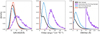 |
Fig. 2. Density distributions of the signal-to-noise at the normalisation wavelength S/N(4020 Å), flux of the Hα emission line F(Hα) and Hα equivalent width EW(Hα) of the main, intensively star-forming, star-forming and passive samples represented by the black, violet, blue and red lines, respectively. |
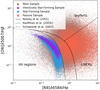 |
Fig. 3. Emission-line flux ratio [NII]λ6583/Hα as a function of [OIII]λ5007/Hβ. Grey, violet, blue and red points represent the main, intensively star-forming, star-forming and passive samples, respectively. Full, dashed and dot-dashed black lines represent the demarcation lines proposed by Kewley et al. (2001), Kauffmann et al. (2003c) and Schawinski et al. (2007), respectively. |
3.2. Total stellar mass, mean age and mean metallicity distributions
Figure 4 shows on the left-hand side panels the distributions of the total stellar mass ever-formed  (top) and presently available
  (bottom) (i.e. after correcting for mass loss through regular stellar evolution) for the MS and SFS galaxy populations. Results show that both codes yield very similar mass distributions. Indeed, the difference between the average total stellar mass from STARLIGHT and FADO is ∼0.02 and 0.01 dex for both masses when it comes to the MS and SFS, respectively. Figure 5 compares the ISFS and PS distributions and shows similar trends, with the difference between the average total stellar mass from STARLIGHT and FADO being ∼0.04 and 0.03 dex, respectively.
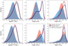 |
Fig. 4. Density distributions of the total stellar mass M⋆ in solar units M⊙ (left-hand side panels), mean stellar age ⟨log t⋆⟩ in years (centred panels) and mean stellar metallicity log⟨Z⋆⟩ in solar units (right-hand side panels). Blue and red colours represent results from FADO and STARLIGHT, respectively, for the main sample (darker colours) and star-forming sample (lighter colours). Top and bottom mass panels display, respectively, the total mass ever-formed throughout the life of the galaxy |


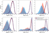 |
Fig. 5. Density distributions of the total stellar mass M⋆ in solar units M⊙ (left-hand side panels), mean stellar age ⟨log t⋆⟩ in years (centred panels) and mean stellar metallicity log⟨Z⋆⟩ in solar units (right-hand side panels). Blue and red colours represent results from FADO and STARLIGHT, respectively, for the passive sample (darker colours) and intensively star-forming sample (lighter colours). Other legend details are identical to those in Fig. 4. |
The age and metallicity distributions of the stellar populations contributing to the best-fit solution can be summarised in terms of their mean values, which can be interpreted as a first order moment of the overall stellar age and metallicity of a given galaxy. Following Cid Fernandes et al. (2005), the mean logarithmic stellar age weighted by light or mass can be defined as, respectively,
 (3)
(3)
 (4)
(4)
where ti is the age of the ith stellar element (i.e. SSP, in this case) in the base library, and γi and μi are its light and mass relative contributions, respectively. The term μi refers to the mass fraction that takes into consideration the amount of stellar matter returned to the interstellar medium through stellar evolution, thus being related to  .
.
Congruously, assuming that Zi represents the relative metallicity contribution of the ith SSP to the best-fit solution, then the mean logarithmic stellar metallicity weighted by light and mass can be defined as, respectively,
 (5)
(5)
 (6)
(6)
Applying these definitions, Fig. 4 shows the distribution of the mean stellar age ⟨log t⋆⟩ (centred panels) and mean stellar metallicity log⟨Z⋆⟩ (right-hand side panels) estimated with FADO (blue) and STARLIGHT (red). The MS distributions show that, overall, the FADO and STARLIGHT results are once more rather similar, with a few noticeable differences: (a) the metallicity distributions of FADO are broader than that of STARLIGHT, (b) the ⟨log t⋆⟩M absolute maxima differ by ∼0.1 dex between FADO and STARLIGHT, and (c) the log⟨Z⋆⟩L and log⟨Z⋆⟩M absolute maxima differ by ∼0.1 dex between codes. Results for the SFS are relatively clearer: (a) the absolute maxima in the ⟨log t⋆⟩L differ by ∼0.1 dex between FADO and STARLIGHT, with the former estimating slightly higher mean ages, (b) FADO displays a broader ⟨log t⋆⟩M distribution than STARLIGHT, and (c) FADO also displays broader metallicity distributions than STARLIGHT, with STARLIGHT preferring values closer to solar metallicity.
It is worth noting that the overall MS mass and age distributions from STARLIGHT illustrated in Fig. 4 are qualitatively in agreement with Mateus et al. (2006), which analysed SDSS DR 7 with STARLIGHT. Moreover, the broadening of the age and metallicity distributions going from STARLIGHT to FADO in MS is also qualitatively similar to that reported by Werle et al. (2020) when going from purely-optical spectroscopy to UV photometry plus optical spectroscopy using STARLIGHT, even though that work is focussed on early-type galaxies.
Comparing results from ISFS and PS in Fig. 5 shows that: (a) FADO and STARLIGHT mean age and metallicity distributions for the PS are very similar, with the main difference being the mass-weighted age distribution of FADO being narrower and with higher maxima in relation to STARLIGHT, (b) STARLIGHT light-weighted age (metallicity) distribution peaks at a lower (higher) value than FADO when it comes the ISFS, and (c) mass-weighted age and metallicity ISFS distributions in both codes are much wider than their light-weighted counterparts.
Interestingly, the light-weighted age distributions for MS in Fig. 4 show two peaks around ∼8.7 and 9.7 dex for both codes, which seem to visually match their SFS and PS distributions, respectively. This could be interpreted at first glance as evidence for the bimodal distribution of galaxies (e.g. Gladders & Yee 2000; Strateva et al. 2001; Blanton et al. 2003; Kauffmann et al. 2003a; Baldry et al. 2004; Mateus et al. 2006). Furthermore, the MS mass-weighted age distribution from STARLIGHT displays two peaks around ∼9.8 and 10.1 dex which, once again, match its SFS and PS distributions. However, the MS mass-weighted age distribution from FADO shows only one prominent peak around ∼10.1 dex, which is congruent with its PS distribution. In addition, the SFS mass-weighted age distribution from FADO (a) is much broader than that of STARLIGHT and (b) displays a conspicuous relative maximum at ∼9.1 dex of unknown origin, also present in the MS distribution.
At least two factors could be behind the differences between the codes regarding these particular features: (a) the different mathematical (e.g. noise treatment and minimisation procedure) and physical approaches of the two codes (e.g. nebular continuum treatment) and (b) the intrinsic degeneracies between the SSPs in the adopted library (e.g. Faber 1972; Worthey 1994; Cid Fernandes et al. 2005). In fact, it is worth considering that CGP19 found that nebular contamination in synthetic SF galaxies leads STARLIGHT to favour best-fit solutions where most of the light comes from a combination of very young and very old SSPs (i.e. bimodal best-fit solutions). A dedicated study exploring, for instance, how variations of the SSPs in the stellar library (e.g. Leitherer et al. 1999; Bruzual & Charlot 2003; Sánchez-Blázquez et al. 2006; Mollá et al. 2009) impact the distributions of these stellar properties would help to clarify the sources behind the MS distribution features observed in each code.
To put the results of Figs. 4–5 into context, it is also worth noting that Cid Fernandes et al. (2005) showed that the original version of STARLIGHT can recover the stellar mass, mean age and mean metallicity within ∼0.1 and ∼0.2 dex when modelling purely stellar synthetic spectra with S/N ∼ 10. Later, Cid Fernandes et al. (2014) used simulations of CALIFA data (Sánchez et al. 2012) and found that the same estimated stellar properties can be affected by uncertainties between ∼0.1 and 0.15 dex related to noise alone and ∼0.15 and 0.25 dex when it comes to changes in the base models. Similar accuracy values were found in CGP19 regarding both FADO and STARLIGHT. Among other factors, these biases can be attributed to the adopted stellar ingredients not adequately representing the wide range of stellar types and their evolutionary stages (e.g. González Delgado & Cid Fernandes 2010; Ge et al. 2019) or possible variations on the stellar initial mass function (e.g. Conroy et al. 2009; Fontanot 2004; Barber et al. 2019).
The average MS, SFS, ISFS and PS population values for mass, age and metallicity are gathered in Table 1 for each code. The differences between codes for total mass, mean age and mean metallicity can go up to ∼0.06 for MS and ∼0.12 dex for SFS, respectively. The most significant difference in MS relates to the average light-weighted age, whereas for SFS the most prominent discrepancies between codes rest on the light-weighted age and metallicity and amount to ∼0.12 and 0.08 dex, respectively. Moreover, the ISFS and PS results in this table show stellar properties differences between codes in the ranges of ∼0.02−0.17 dex for ISFS and ∼0−0.05 dex for PS. Although the main discrepancy in ISFS falls again on the average light-weighted age (∼0.17 dex), the main difference between codes for PS has to do with the average mass-weighted age (∼0.05 dex). The possible origins for these differences are explored in Sect. 3.3. Finally, the working definition for the mass for the remainder of this work is that of  .
.
Average stellar properties of the galaxy samples.
3.3. Light and mass distributions
As the previous results have shown, the mean age ⟨log t⋆⟩ and mean metallicity log⟨Z⋆⟩ parameters are powerful tools to evaluate the stellar properties of galaxies, particularly when grouped in populations of the same type. However, these parameters also lack the detailed information required to understand some of the differences between FADO and STARLIGHT reported in the previous subsection. The same would be true for any ad-hoc binning schema that can be adopted to downscale the best-fit population vector (PV) into more easily manageable parameters. Indeed, a better strategy to study the code differences for each galaxy population is to look into the full information encoded in the best-fit PVs regarding the light and mass contributions of each stellar element.
With this in mind, Fig. 6 shows the light (top panels) and mass relative contributions (bottom panels) of each stellar element (i.e. SSP) in the adopted base library as a function age. The relative contributions of the six metallicities in the base are summed up along each age step (represented by the black squares). These results can be viewed as the light and mass SFHs of each galaxy population, with Fig. A.9 showing their cumulative versions.
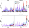 |
Fig. 6. Light (top panels) and mass (bottom panels) relative contributions of the stellar library elements as a function of their age. Black, violet, blue and red lines represent the average results for the MS, ISFS, SFS and PS galaxy populations, respectively, while the surrounding shading denotes their corresponding standard deviation. Black squares represent the age coverage of the adopted stellar library, with the six metallicity values summed at each age step. |
Several results are worth discussing. Firstly, the relative light contributions of young-to-intermediate SSPs with t < 108 yr increases with increasing EW(Hα) in both codes, following the PS→MS→SFS→ISFS sequence. The opposite trend is seen in old SSPs with t > 109 yr. This is to be expected, since young bright stellar populations dominate their older counterparts in terms of light output in ISFS and SFS galaxies, whereas the bulk of stellar content in PS is rather old and considerably less luminous. Secondly, light distribution results show a peak around t ∼ 109 yr in both codes, ranging between ∼5 (ISFS) and 25% (PS). Asari et al. (2007) reported a similar hump around 1 Gyr in the SFR when displayed as a function of stellar age. The authors carried tests with STARLIGHT and found that hump disappears after changing the stellar library of SSPs from STELIB (Bruzual & Charlot 2003), as in this work, to MILES (Sánchez-Blázquez et al. 2006).
The comparison between FADO and STARLIGHT is particularly revealing when it comes to the relative contribution of young and intermediate aged SSPs. Results show that SSPs with ages t < 108 yr contribute with more light in STARLIGHT than in FADO, which is increasingly noticeable with increasing EW(Hα) (PS→MS→SFS→ISFS). Indeed, Fig. A.9 shows that the light contribution in STARLIGHT is greater by 5.41% than in FADO at t = 107 yr for the ISFS, reaching 9.11% around t = 109 yr. This means that STARLIGHT overestimates the relative light contribution of young stellar populations in relation to FADO (or vice versa), thus accounting for the ∼0.12 and 0.17 dex difference in ⟨log t⋆⟩L between the codes for the SFS and ISFS populations, respectively (Table 1).
When it comes to the mass distributions, the differences between the codes are considerably less pronounced. The main reason for this lies in the fact that, in the local universe, most stellar mass is locked into older stellar populations. This is best exemplified by the increasing importance of t > 1010 yr SSPs with decreasing EW(Hα), following the ISFS→SFS→MS→PS sequence. Apart from the peak around t ∼ 109 yr already noted, it is worth observing that STARLIGHT results in the ISFS show higher mass contributions from SSPs at t ∼ 3 × 10⁸ yr than FADO. This seems to be offset by an excess of ∼5% of SSPs with t > 1010 yr, which could explain why the average mean stellar age of STARLIGHT for the SFS (∼9.7 dex) and ISFS (∼9.47 dex) documented in Table 1 is serendipitously identical to that of FADO. In general, these differences between FADO and STARLIGHT when it comes to both the light and mass distributions are somewhat similar to those reported by Werle et al. (2019) when adopting a new version of STARLIGHT that incorporates UV photometry.
Exploring further the information encoded in the PVs, Fig. 7 shows the light (top panels) and mass relative contributions (bottom panels) of each stellar element in base as a function metallicity. In contrast to Fig. 6, the relative contributions of the 25 age steps in the base are now summed along the six metallicities in the base library (represented by the black squares). Other remaining plot details are similar to those of Fig. 6.
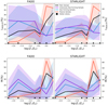 |
Fig. 7. Light (top panels) and mass (bottom panels) relative contributions of the stellar library elements as a function of their metallicity. Black, violet, blue and red lines represent the average results for the MS, ISFS, SFS and PS galaxy populations, respectively, while the surrounding shading denotes their corresponding standard deviation. Black squares represent the metallicity coverage of the adopted stellar library, with the 25 age values summed at each metallicity step. |
The light distributions displayed on the top panels show for both codes that the relative contributions of the lowest metallicities increase with increasing EW(Hα) following PS→MS→SFS→ISFS, with the opposite trend at the highest metallicities. The inversion point occurs somewhere between 2 Z⊙/5 and Z⊙ (i.e. log(Z⋆/Z⊙) = − 0.398 and 0, respectively). Moreover, the best-fit solutions from FADO have higher light contributions from the two lowest metallicities than STARLIGHT, with SSPs with Z⊙/200 and Z⊙/50 (i.e. log(Z⋆/Z⊙)≃ − 2.301 and −1.699, respectively) contributing ∼20−25% in FADO and ∼15−20% in STARLIGHT. This is best displayed in Fig. A.10, which shows that the difference in the relative contribution between FADO and STARLIGHT is already of 8.05% at Z⊙/200 and reaches 13.51% by Z⊙/50 for ISFS. This indicates that STARLIGHT overestimates the metallicity of SF galaxies in comparison to FADO (or vice versa). However, this interpretation is strongly tempered by the particularly large standard deviations observed for SFS and ISFS populations.
As a side note, CGP19 found using synthetic galaxy spectra that STARLIGHT systematically underestimates the light-weighted mean meallicity by up to ∼0.6 dex with decreasing age of the galaxy (i.e. increasing EW(Hα)) for t < 109 yr, whereas the mass-weighted can be underestimated for 107 < t < 109 yr by up to ∼0.6 dex or overestimated by up to ∼0.4 dex for t < 107 yr. Similar results where found in P21. Although the details of these trends depend on the SFH of the models (e.g. instantaneous or continuous), adopted fitting methodology (e.g. including or excluding the emission lines and the Balmer and Paschen discontinuities) and S/N, the important fact to bear in mind is that these tests were carried out assuming a constant solar stellar metallicity of Z⊙ = 0.02. Therefore, metallicity results detailed in Figs. 4 and 7 cannot be easily compared to the results of CGP19 or P21. In contrast, the overall mean age trends documented in this work are compatible to those found in CGP19 or P21.
Finally, the bottom panels of Fig. 7 shows that mass distributions differ very little between codes, in a similar vein to those in Fig. 6. However, it is interesting to note the negligible contribution of two lowest metallicities to the mass when it comes to the PS galaxies, in contrast to both SFS and ISFS. Coupled with the trends observed in the mass distributions as a function age, these results point again to the idea of a bimodal distribution of galaxies (e.g. Gladders & Yee 2000; Strateva et al. 2001; Blanton et al. 2003; Kauffmann et al. 2003a; Baldry et al. 2004).
3.4. Relations between mass, mean age and mean metallicity in star-forming galaxies
Figures 8–10 show in the contour lines the relations between the total stellar mass M⋆, the mean stellar age ⟨log t⋆⟩ and the mean stellar metallicity log⟨Z⋆⟩ for the SFS galaxy population (Figs. A.11–A.13 show similar plots for the MS), with special symbols representing average values for the ISFS, SFS and PS populations.
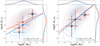 |
Fig. 8. Light (left-hand side panels) and mass-weighted (right-hand side panels) mean stellar metallicity log⟨Z⋆⟩ as a function of total stellar mass M⋆ for the Star-Forming Sample. Blue and red lines and points represent FADO and STARLIGHT results, respectively. The ‘✚’, ‘★’ and ‘✖’ symbols represent the average values for the ISFS, SFS and PS populations, respectively, with standard deviation errorbars. Linear regression results for the SFS population from each code are present in the legend of each plot. |
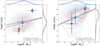 |
Fig. 9. Light (left-hand side panels) and mass-weighted (right-hand side panels) mean stellar age ⟨log t⋆⟩ as a function of total stellar mass M⋆ for the Star-forming Sample. Other legend details are identical to those in Fig. 8. |
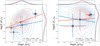 |
Fig. 10. Light (left-hand side panels) and mass-weighted (right-hand side panels) mean stellar metallicity log⟨Z⋆⟩ as a function of mean stellar age ⟨log t⋆⟩ for the star-forming sample. Other legend details are identical to those in Fig. 8. |
The mass-metallicity relation displayed in Fig. 8 shows an increasing divergence between the codes in light-weighted metallicity as EW(Hα) increases and metallicity decreases. This is illustrated by the somewhat steeper linear regression of FADO in comparison with STARLIGHT and the difference between the average values for ISFS, SFS and PS populations. In contrast, both codes show similar results when it comes to the mass-weighted metallicity. Both trends are in keeping with the discussion of Fig. 7.
The mass-age relation in Fig. 9 also shows interesting results. For instance, STARLIGHT shows a systematic light-weighted age underestimation in comparison with FADO with increasing EW(Hα), as shown by the increasing divergence between codes following the sequence PS→SFS→ISFS. This is particularly interesting since the age distributions from both codes are rather similar for SFS. At the same time, FADO shows a mass-weighted mean age distribution that is broader and with a lower absolute maximum when compared to STARLIGHT, even though the average mean stellar ages of the ISFS and SFS samples for each code are very similar, as noted in Table 1 and in Sect. 3.2.
Finally, the age-metallicity relation in Fig. 10 gives another perspective to the age and metallicity differences between codes seen in Figs. 8–9. The contour lines alone clearly illustrate the wider age and metallicity distributions from FADO in comparison with STARLIGHT. The mass-weighted linear regression lines indicate the overall SFS distributions are intrinsically different between codes, even though the average values for each population are rather similar. The FADO results in Fig. 10 are particularly interesting in this regard, since light-weighted metallicity increases with age but its mass-weighted counterpart decreases with its corresponding age. Indeed, the distributions of ⟨log t⋆⟩M and log⟨Z⋆⟩M from FADO are significantly broader that those from STARLIGHT (as illustrated in Fig. 4), with relative maxima at ⟨log t⋆⟩M ∼ 9.1 yr and log⟨Z⋆⟩M ∼ −2.1, weighting towards an anti-correlation between age and metallicity. This anti-correlation can be attributed, at least partly, to the well-known age-metallicity degeneracy, with young metal-rich stellar populations being indistinguishable of old metal-poor populations from the point of view of spectral synthesis (e.g. Faber 1972; O’Connell 1980; Bressan et al. 1996; Pelat 1997a,b; Cid Fernandes et al. 2005). Although this is especially noticeable when it comes to the SFS, the mass-weighted age-metallicity relation presented in Fig. A.13 suggests that this trend is also present in the MS.
4. Discussion
4.1. Impact of the nebular continuum
An important factor to consider in the interpretation of the results presented in Sect. 3 is the potential impact of the nebular continuum modelling approach in each code (or lack thereof) has on the estimated stellar properties of SF galaxies. Moreover, one wonders if this effect can be distinguish from (a) the intrinsic uncertainties (e.g. adequacy of age and metallicity coverages) and degeneracies associated with the adopted physical ingredients (e.g. SSPs, extinction, and kinematics) and (b) the different mathematical methods adopted in each code (e.g. Metropolis algorithm coupled with simulated annealing in STARLIGHT and genetic differential evolution optimisation in FADO).
With this in mind, one of the main objectives of the methodology presented in Sect. 2 was to focus on the impact of nebular continuum modelling in SF galaxies by reducing the number of variables in the code comparison, following a fitting strategy similar to that of CGP19+P21. However, there are important methodological differences between this study and CGP19+P21 that prevent a straightforward comparison between works, such as: (a) the synthetic galaxies analysed in CGP19+P21 have constant solar stellar metallicity, (b) the current work includes two extra sub-solar metallicities in the adopted stellar library, and (c) the most prominent emission lines were masked in STARLIGHT using individual spectral masks in this work, whereas CGP19+P21 adopted a general mask built from STARLIGHT tests using SDSS observations (Cid Fernandes et al. 2005).
Notwithstanding, the question regarding the impact of the nebular continuum modelling approach on the inferred stellar properties remains. In order to address this issue from a different angle, FADO was applied to the SFS and ISFS galaxies in a purely stellar mode (cf. Gomes & Papaderos 2017) using the same input spectra and spectral fitting setup as in STARLIGHT. The objective is to model the spectra using only a combination of stellar components, similarly to STARLIGHT, and compare it with the previous FADO results in which the stellar and nebular spectral continua were fitted self-consistently.
Figure A.14 compares the distributions of the stellar properties using FADO in ‘purely stellar mode’ (STmode) with the results presented in Sect. 3 for FADO in ‘full-consistency mode’ (FCmode) and STARLIGHT. Several interesting results are worth noting: (a) FADO-STmode mass distributions are very similar to those of FADO-FCmode, (b) FADO-STmode light-weighted mean age distribution is close to that of STARLIGHT for SFS and falls between STARLIGHT and FADO-FCmode for ISFS, and (c) FADO-STmode mass-weighted metallicity distributions are slightly more skewed to higher values than FADO-FCmode for both SFS and ISFS, a trend similar to that observed in the STARLIGHT results.
On the one hand, the fact that the FADO-STmode results are in general closer to FADO-FCmode than to STARLIGHT suggests that the code differences documented in Sect. 3 are dominated by the fundamental mathematical and statistical differences between codes (e.g. different minimisation procedures), with different physical ingredients and methods (e.g. different nebular continuum modelling approaches and emission-line masking) playing a secondary role. However, it is reasonable to think that these two factors are likely interconnected, if not mutually dependent.
On the other hand, the FADO-STmode light-weighted age distributions for SFS and ISFS seem to skew from the FADO-FCmode distributions towards those of the STARLIGHT. This is more clearly illustrated in Fig. A.15, which compares the light and mass distributions of the PVs of FADO-STmode with those of STARLIGHT and FADO-FCmode. This figure shows that FADO-STmode overestimates for ISFS the contribution of SSPs younger than ≤107 yr (109) by ∼5.74% (0.88%) in relation to FADO-FCmode, while also overestimating the contribution of SSPs with metallicities ≤Z⊙/200 (Z⊙/50) by ∼9.68% (8.7%). These results show that the nebular continuum modelling approach impacts the FADO results similarly to the light-weighted age trends presented in Sect. 3.3 and, therefore, indirectly suggest that the SFS STARLIGHT results are likely affected by the lack of a nebular continuum modelling recipe (even if its impact is mixed with other uncertainties inherent to population synthesis). One way to rigorously quantify this impact would be to apply STARLIGHT in ‘self-consistent mode’ to these samples of SF galaxies, which obviously is not an option, even considering the code version first presented in López Fernández et al. (2016).
These results highlight an obvious yet elusive idea worth considering during the development of the next generation of spectral synthesis codes. The comparison of new codes, with evermore relevant physical ingredients (e.g. self-consistent dust or AGN treatment), with their older counterparts will necessarily be increasingly complex due to the introduction of more statistical uncertainties and degeneracies between the physical ingredients. Parallel tests with corresponding increasingly physical complexity using synthetic spectral data (e.g. CGP19; P21) will continue to be essential in such an endeavour.
4.2. Potential implications
Assuming that purely stellar modelling in fact leads to an overestimation of mean stellar metallicity with decreasing mass or increasing EW(Hα), this means that the mass-metallicity relation presented in Fig. 8 could become steeper with increasing redshifts as gas reservoirs are both increasingly more abundant and less chemically enriched. This raises the further doubt of how well the synthesis models can mimic the stellar content at large distances. Most commonly adopted evolutionary models are based on stellar libraries of stars in the solar vicinity (e.g. Leitherer et al. 1999; Bruzual & Charlot 2003; Vázquez & Leitherer 2005; Sánchez-Blázquez et al. 2006; Mollá et al. 2009; Vazdekis et al. 2010; Röck et al. 2016), which might not be representative of the stellar populations at high-redshifts, especially when it comes to extremely low metallicities and Population III stars (e.g. Schaerer 2002). The fact that AGN and nebular continua dilute absorption features (e.g. Koski 1978; Cid Fernandes et al. 1998; Moultaka & Pelat 2000; Kauffmann et al. 2003c; Vega et al. 2009; Cardoso et al. 2016, 2017) further exacerbates this problem from the point of view of spectral synthesis. However, this concern is counterbalanced with the increasingly sophisticated theoretical synthesis models (e.g. Coelho et al. 2007, 2020; Mollá et al. 2009; Leitherer et al. 2010; Coelho 2014; Stanway & Eldridge 2019) which can help bridge the gap towards better hybrid evolutionary models.
Moreover, a systematic mean stellar age underestimation when adopting a purely stellar modelling approach has repercussions for the current interpretation of the physical properties of young stellar populations. As noted by Reines et al. (2010), estimating the physical properties (e.g. age and metallicity) of star clusters through population synthesis can only be reliably accomplished when modelling both the nebular continuum and emission-lines. The same is true for galaxies with relatively high specific SFRs in the local universe, such as dwarfs (e.g. Papaderos et al. 1998; Papaderos & Östlin 2012) and ‘green peas’ (e.g. Izotov et al. 2011; Amorín et al. 2012), or at higher redshifts (e.g. Zackrisson et al. 2008; Schaerer & de Barros 2009).
From a different perspective, variations in the emission-line measurements could impact SFR estimations and, thus, indirectly affect estimations of the cosmic SF history (Panter et al. 2007). The fact that FADO measures emission-lines after subtracting the nebular continuum means that the EWs of the Balmer lines will always be greater than those based on a purely stellar modelling approach. At the same time, SFR estimators based on emission-line fluxes are not expected to change since the modelling (or not) of the nebular continuum does not impact the measured fluxes.
5. Summary and conclusions
The population synthesis code FADO (Gomes & Papaderos 2017, 2018) was applied to the main sample of galaxies from the SDSS (York et al. 2000) DR7 (Abazajian et al. 2009) with the aim of re-evaluating the relations between the main stellar properties of galaxies (e.g. mass, mean age, and mean metallicity), particularly those of SF galaxies. The main reason for such re-analysis is the fact that FADO is the first publicly available population synthesis tool to self-consistently model both the stellar and nebular continua. In fact, previous studies adopted purely stellar population synthesis codes (e.g. STARLIGHT, Cid Fernandes et al. 2005) to infer the physical properties of galaxies, regardless of their spectral and morphological type (e.g. Kauffmann et al. 2003b; Panter et al. 2003; Cid Fernandes et al. 2005; Asari et al. 2007; Tojeiro et al. 2009).
Comparing the physical properties inferred by the population synthesis codes FADO and STARLIGHT for four distinct galaxy samples: main sample (i.e. general population of galaxies), star-forming (EW(Hα) > 3), intensively star-forming (EW(Hα) > 75), and passive (EW(Hα) < 0.5), shows that:
-
Mass distributions for the different galaxy samples are similar between FADO and STARLIGHT.
-
Mean age and mean metallicity distributions in SFS from FADO are broader than those of STARLIGHT, especially when weighted by mass. Moreover, the average light-weighted age of STARLIGHT is lower by ∼0.17 dex than FADO for ISFS galaxies, whereas the light-weighted metallicity of STARLIGHT is ∼0.13 dex higher than FADO.
-
Even though both codes show very similar mass, age and metallicity distributions for the PS population of galaxies, FADO displays a narrower and higher mass-weighted age peak than STARLIGHT.
-
Cumulative light distributions of the best-fit PVs as a function of age show for ISFS that the contribution of SSPs with t < 107 yr is greater by 5.41% in STARLIGHT than in FADO, reaching 9.11% for SSPs younger than t < 109 yr, which means that STARLIGHT overestimates the relative light contribution of young stellar populations in comparison with FADO (or vice versa). Moreover, cumulative light distributions as a function of metallicity indicate that the light difference between FADO and STARLIGHT for ISFS is ∼8.05% and 13.51% for Z⋆ ≤ Z⊙/200 and Z⊙/50 (i.e. the lowest metallicities in the adopted stellar library), respectively. This means that FADO underestimates the metallicity when compared to STARLIGHT (or vice versa). Meanwhile, mass distributions as a function of age and metallicity from both codes are very similar for all samples, except that STARLIGHT once again fits more SSPs with ages t < 109 yr than FADO for both SFS and ISFS.
-
Comparing the different relation permutations between total mass, mean age and mean metallicity shows all previous results in a more general way: (a) light-weighted age and metallicity differences between codes increases with increasing EW(Hα) and decreasing total mass, (b) mass-weighted age and metallicity differences between codes are minimal, except for the age underestimation of STARLIGHT in relation to FADO when it comes specifically to PS galaxies, and (c) SFS age and metallicity distributions of FADO are broader than those of STARLIGHT.
These results indicate that the nebular continuum modelling approach significantly impacts the inferred stellar properties of SF galaxies, even if the negative effects of a purely stellar modelling approach are mixed with other uncertainties and degeneracies associated with population synthesis synthesis. For instance, this work found that the modelling of the nebular continuum with FADO yields steeper light-weighted mass-metallicity correlation and a flatter light-weighted mass-age correlation when compared to STARLIGHT, a purely stellar population synthesis code. Among other potential implications, this means that the stellar populations of low-mass galaxies in the local universe with relatively high specific SFRs are both more metal poor and older than previously thought. These results are particularly relevant in light of future high-resolution spectroscopic surveys at higher redshifts, such as the 4MOST-4HS (de Jong et al. 2019) and MOONS (Cirasuolo et al. 2011, 2020; Maiolino et al. 2020), for which the fraction of intensively SF galaxies is expected to be higher.
The same version adopted in this work. Not to be confused with the one introduced by López Fernández et al. (2016), which combines UV photometry with spectral fitting in the optical.
Version 1b: http://www.spectralsynthesis.org
Version 4: http://www.starlight.ufsc.br
Acknowledgments
The authors thank the anonymous referee for valuable comments and suggestions, and colleagues Andrew Humphrey, Isreal Matute and Tom Scott (Instituto de Astrofísica e Ciências do Espaço; IA) for engaging scientific discussions. This work was supported by Fundaçño para a Cióncia e a Tecnologia (FCT) through the research grants UID/FIS/04434/2019, UIDB/04434/2020 and UIDP/04434/2020. L.S.M.C. acknowledges support by the project ‘Enabling Green E-science for the SKA Research Infrastructure (ENGAGE SKA)’ (reference POCI-01-0145-FEDER-022217) funded by COMPETE 2020 and FCT. J.M.G. is supported by the DL 57/2016/CP1364/CT0003 contract and acknowledges the previous support by the fellowships CIAAUP-04/2016-BPD in the context of the FCT project UID/FIS/04434/2013 and POCI-01-0145-FEDER-007672, and SFRH/BPD/66958/2009 funded by FCT and POPH/FSE (EC). P.P. is supported by the project “Identifying the Earliest Supermassive Black Holes with ALMA (IdEaS with ALMA)” (PTDC/FIS-AST/29245/2017). C.P. acknowledges support from DL 57/2016 (P2460) from the ‘Departamento de Física, Faculdade de Cióncias da Universidade de Lisboa’. A.P.A. acknowledges support from the Fundaçño para a Cióncia e a Tecnologia (FCT) through the work Contract No. 2020.03946.CEECIND, and through the FCT project EXPL/FIS-AST/1085/2021. J.A. acknowledges financial support from the Science and Technology Foundation (FCT, Portugal) through research grants UIDB/04434/2020 and UIDP/04434/2020. P.L. is supported by the DL 57/2016/CP1364/CT0010 contract. Funding for the SDSS and SDSS-II has been provided by the Sloan Foundation, the Participating Institutions, the National Science Foundation, the US Department of Energy, the National Aeronautics and Space Administration, the Japanese Monbukagakusho, the Max Planck Society, and the Higher Education Funding Council for England. The SDSS website is http://www.sdss.org/. The SDSS is managed by the Astrophysical Research Consortium for the Participating Institutions. The Participating Institutions are the American Museum of Natural History, Astrophysical Institute Potsdam, University of Basel, University of Cambridge, Case Western Reserve University, University of Chicago, Drexel University, Fermilab, the Institute for Advanced Study, the Japan Participation Group, Johns Hopkins University, the Joint Institute for Nuclear Astrophysics, the Kavli Institute for Particle Astrophysics and Cosmology, the Korean Scientist Group, the Chinese Academy of Sciences (LAMOST), Los Alamos National Laboratory, the Max-Planck-Institute for Astronomy (MPIA), the Max-Planck-Institute for Astrophysics (MPA), New Mexico State University, Ohio State University, University of Pittsburgh, University of Portsmouth, Princeton University, the United States Naval Observatory, and the University of Washington.
References
- Abazajian, K. N., Adelman-McCarthy, J. K., & Agüeros, M. A. 2009, ApJS, 182, 543 [NASA ADS] [CrossRef] [Google Scholar]
- Alongi, M., Bertelli, G., Bressan, A., et al. 1993, A&AS, 97, 851 [NASA ADS] [Google Scholar]
- Anders, P., & Fritze-v Alvensleben, U. 2003, A&A, 401, 1063 [NASA ADS] [CrossRef] [EDP Sciences] [Google Scholar]
- Amorín, R., Pérez-Montero, E., Vílchez, J. M., et al. 2012, ApJ, 749, 17 [NASA ADS] [CrossRef] [Google Scholar]
- Asari, N. V., Cid Fernandes, R., Stasińska, G., et al. 2007, MNRAS, 381, 263 [Google Scholar]
- Baldry, I. K., Glazebrook, K., Brinkmann, J., et al. 2004, ApJ, 600, 681 [Google Scholar]
- Baldwin, J. A., Phillips, M. M., & Terlevich, R. 1981, PASP, 93, 5 [Google Scholar]
- Barber, C., Schaye, J., & Crain, R. A. 2019, MNRAS, 482, 2515 [NASA ADS] [CrossRef] [Google Scholar]
- Blanton, M. R., Hogg, D. W., Bahcall, N. A., et al. 2003, ApJ, 594, 186 [NASA ADS] [CrossRef] [Google Scholar]
- Bressan, A., Fagotto, F., Bertelli, G., et al. 1993, A&AS, 100, 647 [Google Scholar]
- Bressan, A., Chiosi, C., & Tantalo, R. 1996, A&A, 311, 425 [NASA ADS] [Google Scholar]
- Brinchmann, J., Charlot, S., White, S. D. M., et al. 2004, MNRAS, 351, 1151 [Google Scholar]
- Bruzual, G., & Charlot, S. 2003, MNRAS, 344, 1000 [NASA ADS] [CrossRef] [Google Scholar]
- Calzetti, D., Armus, L., Bohlin, R. C., et al. 2000, ApJ, 533, 682 [NASA ADS] [CrossRef] [Google Scholar]
- Cai, W., Zhao, Y., Zhang, H.-X., et al. 2020, ApJ, 903, 58 [NASA ADS] [CrossRef] [Google Scholar]
- Cai, W., Zhao, Y.-H., & Bai, J.-M. 2021, Res. Astron. Astrophys., 21, 204 [CrossRef] [Google Scholar]
- Cardelli, J. A., Clayton, G. C., & Mathis, J. S. 1989, ApJ, 345, 245 [Google Scholar]
- Cardoso, L. S. M., Gomes, J. M., & Papaderos, P. 2016, A&A, 594, L2 [NASA ADS] [CrossRef] [EDP Sciences] [Google Scholar]
- Cardoso, L. S. M., Gomes, J. M., & Papaderos, P. 2017, A&A, 604, A99 [NASA ADS] [CrossRef] [EDP Sciences] [Google Scholar]
- Cardoso, L. S. M., Gomes, J. M., & Papaderos, P. 2019, A&A, 622, A56 [NASA ADS] [CrossRef] [EDP Sciences] [Google Scholar]
- Chabrier, G. 2003, ApJ, 586, 133 [Google Scholar]
- Cid Fernandes, R., Jr., Storchi-Bergmann, T., Schmitt, H. R. 1998, MNRAS, 297, 579 [CrossRef] [Google Scholar]
- Cid Fernandes, R., Mateus, A., Sodré, L., et al. 2005, MNRAS, 358, 363 [CrossRef] [Google Scholar]
- Cid Fernandes, R., Stasińska, G., Mateus, A., et al. 2011, MNRAS, 413, 1687 [NASA ADS] [CrossRef] [Google Scholar]
- Cid Fernandes, R., González Delgado, R. M., García Benito, R., et al. 2014, A&A, 561, A130 [NASA ADS] [CrossRef] [EDP Sciences] [Google Scholar]
- Cimatti, A., Daddi, E., & Renzini, A. 2006, A&A, 453, L29 [NASA ADS] [CrossRef] [EDP Sciences] [Google Scholar]
- Cirasuolo, M., Afonso, J., Bender, R., et al. 2011, The Messenger, 145, 11 [Google Scholar]
- Cirasuolo, M., Fairley, A., Rees, P., et al. 2020, The Messenger, 180, 10 [NASA ADS] [Google Scholar]
- Coelho, P. 2014, MNRAS, 440, 1027 [NASA ADS] [CrossRef] [Google Scholar]
- Coelho, P., Bruzual, G., Charlot, S., et al. 2007, MNRAS, 382, 498 [NASA ADS] [CrossRef] [Google Scholar]
- Coelho, P., Bruzual, G., & Charlot, S. 2020, MNRAS, 491, 2025 [NASA ADS] [CrossRef] [Google Scholar]
- Cooper, M. C., Gallazzi, A., Newman, J. A., et al. 2010, MNRAS, 402, 1942 [NASA ADS] [CrossRef] [Google Scholar]
- Cowie, L. L., Songaila, A., Hu, E. M., et al. 1995, AJ, 112, 839 [Google Scholar]
- Conroy, C., Gunn, J. E., & White, M. 2009, ApJ, 699, 486 [Google Scholar]
- de Jong, R. S., Agertz, O., Berbel, A. A., et al. 2019, The Messenger, 175, 3 [NASA ADS] [Google Scholar]
- Duarte Puertas, S., Vilchez, J. M., Iglesias-Páramo, J., et al. 2017, A&A, 599, A71 [NASA ADS] [CrossRef] [EDP Sciences] [Google Scholar]
- Faber, S. M. 1972, A&A, 20, 361 [NASA ADS] [Google Scholar]
- Fagotto, F., Bressan, A., Bertelli, G., et al. 1994a, A&AS, 104, 365 [Google Scholar]
- Fagotto, F., Bressan, A., Bertelli, G., et al. 1994b, A&AS, 105, 29 [Google Scholar]
- Ferland, G. J., Korista, K. T., Verner, D. A., et al. 1998, PASP, 110, 761 [Google Scholar]
- Ferland, G. J., Porter, R. L., van Hoof, P. A. M., et al. 2013, Rev. Mex. Astron. Astrofis., 49, 137 [Google Scholar]
- Fontanot, F. 2004, MNRAS, 442, 3138 [Google Scholar]
- Ge, J., Mao, S., Lu, Y., et al. 2019, MNRAS, 485, 1675 [NASA ADS] [CrossRef] [Google Scholar]
- Girardi, L., Bressan, A., Chiosi, C., et al. 1996, A&AS, 117, 113 [NASA ADS] [CrossRef] [EDP Sciences] [Google Scholar]
- Gladders, M. D., & Yee, H. K. C. 2000, AJ, 120, 2148 [NASA ADS] [CrossRef] [Google Scholar]
- Gomes, J. M., & Papaderos, P. 2017, A&A, 603, A63 [NASA ADS] [CrossRef] [EDP Sciences] [Google Scholar]
- Gomes, J. M., & Papaderos, P. 2018, A&A, 618, C3 [NASA ADS] [CrossRef] [EDP Sciences] [Google Scholar]
- Gomes, J. M., Papaderos, P., Vílchez, J. M., et al. 2016a, A&A, 585, A92 [NASA ADS] [CrossRef] [EDP Sciences] [Google Scholar]
- Gomes, J. M., Papaderos, P., Vílchez, J. M., et al. 2016b, A&A, 586, A22 [NASA ADS] [CrossRef] [EDP Sciences] [Google Scholar]
- González Delgado, R. M., & Cid Fernandes, R. 2010, MNRAS, 403, 797 [CrossRef] [Google Scholar]
- Green, A. W., Glazebrook, K., Gilbank, D. G., et al. 2017, MNRAS, 470, 639 [CrossRef] [Google Scholar]
- Gunawardhana, M. L. P., Brinchmann, J., Weilbacher, P. M., et al. 2020, MNRAS, 497, 3860 [NASA ADS] [CrossRef] [Google Scholar]
- Hao, L., Strauss, M. A., Tremonti, C. A., et al. 2005, AJ, 129, 1783 [Google Scholar]
- Heavens, A., Panter, B., Jimenez, R., et al. 2004, Nature, 428, 625 [CrossRef] [Google Scholar]
- Hogg, D. W., Blanton, M. R., Brinchmann, J., et al. 2004, ApJ, 601, 29 [Google Scholar]
- Izotov, Y. I., Guseva, N. G., & Thuan, T. X. 2011, ApJ, 727, 161 [NASA ADS] [CrossRef] [Google Scholar]
- Kauffmann, G., Heckman, T. M., White, S. D. M., et al. 2003a, MNRAS, 341, 54 [Google Scholar]
- Kauffmann, G., Heckman, T. M., White, S. D. M., et al. 2003b, MNRAS, 341, 33 [Google Scholar]
- Kauffmann, G., Heckman, T. M., Tremonti, C., et al. 2003c, MNRAS, 346, 1055 [Google Scholar]
- Kewley, L. J., Dopita, M. A., Sutherland, R. S., Heisler, C. A., & Trevena, J. 2001, ApJ, 556, 121 [Google Scholar]
- Koleva, M., Prugniel, Ph., Bouchard, A., et al. 2009, A&A, 501, 1269 [CrossRef] [EDP Sciences] [Google Scholar]
- Koski, A. T. 1978, ApJ, 223, 56 [NASA ADS] [CrossRef] [Google Scholar]
- Krüger, H., Fritze-v Alvensleben, U., & Loose, H. H. 1995, A&A, 303, 41 [NASA ADS] [Google Scholar]
- Leitherer, C., Schaerer, D., Goldader, J. D., et al. 1999, ApJS, 123, 3 [Google Scholar]
- Leitherer, C., Ortiz Otálvaro, P. A., Bresolin, F., et al. 2010, ApJS, 189, 309 [Google Scholar]
- Lequeux, J., Peimbert, M., Rayo, J. F., et al. 1979, A&A, 80, 155 [NASA ADS] [Google Scholar]
- López Fernández, R., Cid Fernandes, R., González Delgado, R. M., et al. 2016, MNRAS, 458, 184 [CrossRef] [Google Scholar]
- Kuźmicz, A., Czerny, B., & Wildy, C. 2019, A&A, 624, A91 [NASA ADS] [CrossRef] [EDP Sciences] [Google Scholar]
- Maiolino, R., Cirasuolo, M., Afonso, J., et al. 2020, The Messenger, 180, 24 [NASA ADS] [Google Scholar]
- Martín-Manjón, M. L., García-Vargas, M. L., Mollá, M., et al. 2010, MNRAS, 403, 2012 [CrossRef] [Google Scholar]
- Mateus, A., Sodré, L., Cid Fernandes, R., et al. 2006, MNRAS, 370, 721 [NASA ADS] [CrossRef] [Google Scholar]
- Mollá, M., García-Vargas, M. L., & Bressan, A. 2009, MNRAS, 398, 451 [CrossRef] [Google Scholar]
- Moultaka, J., & Pelat, D. 2000, MNRAS, 314, 409 [NASA ADS] [CrossRef] [Google Scholar]
- Noeske, K. G., Weiner, B. J., Faber, S. M., et al. 2007, ApJ, 660, 43 [Google Scholar]
- O’Connell, R. W. 1980, ApJ, 236, 430 [CrossRef] [Google Scholar]
- Ocvirk, P., Pichon, C., Lançon, A., & Thiébaut, E. 2006a, MNRAS, 365, 46 [Google Scholar]
- Ocvirk, P., Pichon, C., Lançon, A., & Thiébaut, E. 2006b, MNRAS, 365, 74 [Google Scholar]
- Pacifici, C., da Cunha, E., Charlot, S., et al. 2015, MNRAS, 447, 786 [NASA ADS] [CrossRef] [Google Scholar]
- Panter, B., Heavens, A. F., & Jimenez, R. 2003, MNRAS, 343, 1145 [Google Scholar]
- Panter, B., Jimenez, R., Heavens, A. F., et al. 2007, MNRAS, 378, 1550 [NASA ADS] [CrossRef] [Google Scholar]
- Papaderos, P., & Östlin, G. 2012, A&A, 537, A126 [NASA ADS] [CrossRef] [EDP Sciences] [Google Scholar]
- Papaderos, P., Izotov, Y. I., Fricke, K. J., et al. 1998, A&A, 338, 43 [NASA ADS] [Google Scholar]
- Pappalardo, C., Cardoso, L. S. M., Gomes, J. M., et al. 2021, A&A, 651, A99 [NASA ADS] [CrossRef] [EDP Sciences] [Google Scholar]
- Pelat, D. 1997a, MNRAS, 284, 365 [NASA ADS] [CrossRef] [Google Scholar]
- Pelat, D. 1997b, MNRAS, 299, 877 [Google Scholar]
- Pérez, E., Cid Fernandes, R., González Delgado, R. M., et al. 2013, ApJ, 764, 1 [Google Scholar]
- Reines, A. E., Nidever, D. L., Whelan, D. G., et al. 2010, ApJ, 708, 26 [NASA ADS] [CrossRef] [Google Scholar]
- Ribeiro, B., Lobo, C., Antón, S., et al. 2016, MNRAS, 456, 3899 [NASA ADS] [CrossRef] [Google Scholar]
- Richards, S. N., Bryant, J. J., Croom, S. M., et al. 2016, MNRAS, 455, 2826 [NASA ADS] [CrossRef] [Google Scholar]
- Röck, B., Vazdekis, A., Ricciardelli, E., et al. 2016, A&A, 589, A73 [NASA ADS] [CrossRef] [EDP Sciences] [Google Scholar]
- Rosa, D. A., Milone, A. C., Krabbe, A. C., et al. 2018, Ap&SS, 363, 131 [NASA ADS] [CrossRef] [Google Scholar]
- Sánchez, S. F., Kennicutt, R. C., Gil de Paz, A., et al. 2012, A&A, 538, A8 [Google Scholar]
- Sánchez-Blázquez, P., Peletier, R. F., Jiménez-Vicente, J., et al. 2006, MNRAS, 371, 703 [Google Scholar]
- Sánchez-Blázquez, P., Rosales-Ortega, F. F., Méndez-Abreu, J., et al. 2014, A&A, 570, A6 [NASA ADS] [CrossRef] [EDP Sciences] [Google Scholar]
- Schaerer, D. 2002, A&A, 382, 28 [NASA ADS] [CrossRef] [EDP Sciences] [Google Scholar]
- Schaerer, D., & de Barros, S. 2009, A&A, 502, 423 [NASA ADS] [CrossRef] [EDP Sciences] [Google Scholar]
- Schawinski, K., Thomas, D., Sarzi, M., et al. 2007, MNRAS, 382, 1415 [Google Scholar]
- Schlafly, E. F., & Finkbeiner, D. P. 2011, ApJ, 737, 13 [NASA ADS] [CrossRef] [Google Scholar]
- Schlegel, D. J., Finkbeiner, D. P., & Davis, M. 1998, ApJ, 500, 525 [Google Scholar]
- Stanway, E. R., & Eldridge, J. J. 2019, A&A, 621, A13 [Google Scholar]
- Strateva, I., Ivezic, Z., Knapp, G. R., et al. 2001, AJ, 122, 1861 [CrossRef] [Google Scholar]
- Tojeiro, R., Heavens, A. F., Jimenez, R., & Panter, B. 2007, MNRAS, 11, 1252 [NASA ADS] [CrossRef] [Google Scholar]
- Tojeiro, R., Wilkins, S., Heavens, A. F., et al. 2009, ApJS, 185, 1 [NASA ADS] [CrossRef] [Google Scholar]
- Torres-Papaqui, J. P., Coziol, R., Ortega-Minakata, R. A., et al. 2012, ApJ, 754, 144 [NASA ADS] [CrossRef] [Google Scholar]
- Tremonti, C. A., Heckman, T. M., Kauffmann, G., et al. 2004, ApJ, 613, 898 [Google Scholar]
- Vazdekis, A., Sánchez-Blázquez, P., Falcón-Barroso, J., et al. 2010, MNRAS, 404, 1639 [NASA ADS] [Google Scholar]
- Vázquez, G. A., & Leitherer, C. 2005, ApJ, 621, 695 [Google Scholar]
- Vega, L. R., Asari, N. V., Cid Fernandes, R., et al. 2009, MNRAS, 393, 846 [NASA ADS] [CrossRef] [Google Scholar]
- Werle, A., Cid Fernandes, R., Vale Asari, N., et al. 2019, MNRAS, 483, 2382 [Google Scholar]
- Werle, A., Cid Fernandes, R., Vale Asari, N., et al. 2020, MNRAS, 497, 3251 [NASA ADS] [CrossRef] [Google Scholar]
- Worthey, G. 1994, ApJS, 95, 107 [Google Scholar]
- York, D. G., Adelman, J., Anderson, J. E., Jr., et al. 2000, ApJ, 120, 1579 [CrossRef] [Google Scholar]
- Zackrisson, E., Bergvall, N., Olofsson, K., et al. 2001, A&A, 375, 814 [NASA ADS] [CrossRef] [EDP Sciences] [Google Scholar]
- Zackrisson, E., Bergvall, N., & Leitet, E. 2008, ApJ, 676, L9 [NASA ADS] [CrossRef] [Google Scholar]
- Zhong, G. H., Liang, Y. C., Hammer, F., et al. 2010, A&A, 520, A69 [NASA ADS] [CrossRef] [EDP Sciences] [Google Scholar]
Appendix A: Supplements
Figures A.1–A.8 show the results of the FADO and STARLIGHT spectral fits for two randomly selected spectra from each galaxy population defined in Subsection 3.1: Main Sample, Star-Forming Sample, Intensively Star-Forming Sample and Passive Sample, respectively. The light-weighted SFH results for the SFS (Figures A.3 & A.4) and ISFS spectra (Figures A.5 & A.6) show in particular the differences between FADO and STARLIGHT, with the relative contribution of SSPs younger than 100 Myr in STARLIGHT being much more prominent than those in the FADO results.
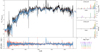 |
Fig. A.1. Spectral modelling results from STARLIGHT and FADO for the SDSS spectrum ‘51630-0266-004’ in the Main Sample. The format and other legend details are identical to those in Fig. 1. |
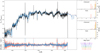 |
Fig. A.2. Spectral modelling results from STARLIGHT and FADO for the SDSS spectrum ‘51630-0266-011’ in the Main Sample. The format and other legend details are identical to those in Fig. 1. |
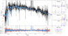 |
Fig. A.3. Spectral modelling results from STARLIGHT and FADO for the SDSS spectrum ‘51630-0266-014’ in the Star-Forming Sample. The format and other legend details are identical to those in Fig. 1. |
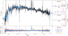 |
Fig. A.4. Spectral modelling results from STARLIGHT and FADO for the SDSS spectrum ‘51630-0266-017’ in the Star-Forming Sample. The format and other legend details are identical to those in Fig. 1. |
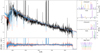 |
Fig. A.5. Spectral modelling results from STARLIGHT and FADO for the SDSS spectrum ‘51957-0273-573’ in the Intensively Star-Forming Sample. The format and other legend details are identical to those in Fig. 1. |
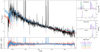 |
Fig. A.6. Spectral modelling results from STARLIGHT and FADO for the SDSS spectrum ‘51957-0273-625’ in the Intensively Star-Forming Sample. The format and other legend details are identical to those in Fig. 1. |
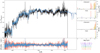 |
Fig. A.7. Spectral modelling results from STARLIGHT and FADO for the SDSS spectrum ‘51630-0266-491’ in the Passive Sample. The format and other legend details are identical to those in Fig. 1. |
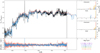 |
Fig. A.8. Spectral modelling results from STARLIGHT and FADO for the SDSS spectrum ‘51630-0266-493’ in the Passive Sample. The format and other legend details are identical to those in Fig. 1. |
Figures A.9 and A.10 show the cumulative versions of Figures 6 and 7 with the light and mass contributions being summed with increasing age and metallicity, respectively. The fact that the assembly histories for the PS are practical identical between codes is an important sign that both codes estimate similar SFHs for galaxies with negligible to none nebular contribution to the continuum (EW(Hα) < 0.5 Å).
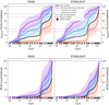 |
Fig. A.9. Cumulative light (top panels) and mass (bottom panels) relative contributions of the stellar library elements as a function of their age. Other legend details are identical to those in Fig. 6. |
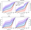 |
Fig. A.10. Cumulative light (top panels) and mass (bottom panels) relative contributions of the stellar library elements as a function of their metallicity. Other legend details are identical to those in Fig. 7. |
Figures A.11, A.12 and A.13 shows the relations between the total stellar mass, mean stellar age and mean stellar metallicity for the MS of galaxies for both codes. The contour and histograms show that the distributions for the three stellar properties in both codes are similar, with the only interesting difference being that FADO displays a slightly larger light-weighted mean metallicity distribution than STARLIGHT.
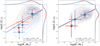 |
Fig. A.11. Mean stellar metallicity and log⟨Z⋆⟩ as a function of total stellar mass M⋆for the Main Sample. Blue and red lines and points represent FADO and STARLIGHT results, respectively. The ‘✚’, ‘★’ and ‘✖’ symbols represent the average values for the ISFS, SFS and PS populations, respectively, with standard deviation errorbars. Linear regression results for the MS population from each code are present in the legend of each plot. |
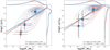 |
Fig. A.12. Mean stellar age ⟨log t⋆⟩ as a function of total stellar mass M⋆ for the Main Sample. Other legend details are identical to those in Fig. A.11. |
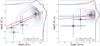 |
Fig. A.13. Mean stellar metallicity and log⟨Z⋆⟩ as a function of mean stellar age ⟨log t⋆⟩ for the Main Sample. Other legend details are identical to those in Fig. A.11. |
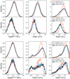 |
Fig. A.14. Density distributions of the total stellar mass M⋆ in solar units M⊙ (left-hand side panels), mean stellar age ⟨log t⋆⟩ in years (centred panels) and mean stellar metallicity log⟨Z⋆⟩ in solar units (right-hand side panels). Red, blue and black lines represent results from STARLIGHT and FADO in ‘full-consistency mode’ (FCmode) and ‘purely stellar mode’ (STmode), respectively. Moreover, top and bottom row panels in each section represent results for the Star-Forming (SFS) and Intensively Star-Forming Samples (ISFS), respectively. |
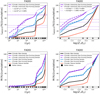 |
Fig. A.15. Cumulative light (top panels) and mass (bottom panels) relative contributions of the stellar library elements as a function of their age (left-hand side panels) and metallicity (right-hand side panels). Full and dashed lines represent FADO results in ‘full-consistency mode’ (FCmode) and ‘purely stellar mode’ (STmode), respectively. Black squares on the left and right-hand side panels represent the age and metallicity coverages of the adopted stellar library, respectively. Other legend details are identical to those in Fig. 6. |
All Tables
All Figures
|
Fig. 1. Spectral modelling results for the SDSS DR7 spectrum ‘52912-1424-151’ using the spectral synthesis codes FADO and STARLIGHT. Main panel: black, blue and red lines represent the galaxy input spectrum and the best-fit solutions from FADO and STARLIGHT, respectively. Bottom panel: blue and red lines represent the residual spectra of FADO and STARLIGHT, respectively, that result from subtracting the best-fit solutions from the input spectrum. Top right-hand side panels: light fractions L4020 Å at the normalisation wavelength λ0 = 4020 Å as a function of the age of the SSPs in the best-fit solution of STARLIGHT (top) and FADO (bottom), with colour coding representing metallicity. Bottom right-hand side panels: mass fractions of the SSPs fitted by STARLIGHT (top) and FADO (bottom). The black vertical ticks on the top of the x-axes represent the age coverage of the adopted stellar library. |
| In the text | |
|
Fig. 2. Density distributions of the signal-to-noise at the normalisation wavelength S/N(4020 Å), flux of the Hα emission line F(Hα) and Hα equivalent width EW(Hα) of the main, intensively star-forming, star-forming and passive samples represented by the black, violet, blue and red lines, respectively. |
| In the text | |
|
Fig. 3. Emission-line flux ratio [NII]λ6583/Hα as a function of [OIII]λ5007/Hβ. Grey, violet, blue and red points represent the main, intensively star-forming, star-forming and passive samples, respectively. Full, dashed and dot-dashed black lines represent the demarcation lines proposed by Kewley et al. (2001), Kauffmann et al. (2003c) and Schawinski et al. (2007), respectively. |
| In the text | |
|
Fig. 4. Density distributions of the total stellar mass M⋆ in solar units M⊙ (left-hand side panels), mean stellar age ⟨log t⋆⟩ in years (centred panels) and mean stellar metallicity log⟨Z⋆⟩ in solar units (right-hand side panels). Blue and red colours represent results from FADO and STARLIGHT, respectively, for the main sample (darker colours) and star-forming sample (lighter colours). Top and bottom mass panels display, respectively, the total mass ever-formed throughout the life of the galaxy |
| In the text | |
|
Fig. 5. Density distributions of the total stellar mass M⋆ in solar units M⊙ (left-hand side panels), mean stellar age ⟨log t⋆⟩ in years (centred panels) and mean stellar metallicity log⟨Z⋆⟩ in solar units (right-hand side panels). Blue and red colours represent results from FADO and STARLIGHT, respectively, for the passive sample (darker colours) and intensively star-forming sample (lighter colours). Other legend details are identical to those in Fig. 4. |
| In the text | |
|
Fig. 6. Light (top panels) and mass (bottom panels) relative contributions of the stellar library elements as a function of their age. Black, violet, blue and red lines represent the average results for the MS, ISFS, SFS and PS galaxy populations, respectively, while the surrounding shading denotes their corresponding standard deviation. Black squares represent the age coverage of the adopted stellar library, with the six metallicity values summed at each age step. |
| In the text | |
|
Fig. 7. Light (top panels) and mass (bottom panels) relative contributions of the stellar library elements as a function of their metallicity. Black, violet, blue and red lines represent the average results for the MS, ISFS, SFS and PS galaxy populations, respectively, while the surrounding shading denotes their corresponding standard deviation. Black squares represent the metallicity coverage of the adopted stellar library, with the 25 age values summed at each metallicity step. |
| In the text | |
|
Fig. 8. Light (left-hand side panels) and mass-weighted (right-hand side panels) mean stellar metallicity log⟨Z⋆⟩ as a function of total stellar mass M⋆ for the Star-Forming Sample. Blue and red lines and points represent FADO and STARLIGHT results, respectively. The ‘✚’, ‘★’ and ‘✖’ symbols represent the average values for the ISFS, SFS and PS populations, respectively, with standard deviation errorbars. Linear regression results for the SFS population from each code are present in the legend of each plot. |
| In the text | |
|
Fig. 9. Light (left-hand side panels) and mass-weighted (right-hand side panels) mean stellar age ⟨log t⋆⟩ as a function of total stellar mass M⋆ for the Star-forming Sample. Other legend details are identical to those in Fig. 8. |
| In the text | |
|
Fig. 10. Light (left-hand side panels) and mass-weighted (right-hand side panels) mean stellar metallicity log⟨Z⋆⟩ as a function of mean stellar age ⟨log t⋆⟩ for the star-forming sample. Other legend details are identical to those in Fig. 8. |
| In the text | |
|
Fig. A.1. Spectral modelling results from STARLIGHT and FADO for the SDSS spectrum ‘51630-0266-004’ in the Main Sample. The format and other legend details are identical to those in Fig. 1. |
| In the text | |
|
Fig. A.2. Spectral modelling results from STARLIGHT and FADO for the SDSS spectrum ‘51630-0266-011’ in the Main Sample. The format and other legend details are identical to those in Fig. 1. |
| In the text | |
|
Fig. A.3. Spectral modelling results from STARLIGHT and FADO for the SDSS spectrum ‘51630-0266-014’ in the Star-Forming Sample. The format and other legend details are identical to those in Fig. 1. |
| In the text | |
|
Fig. A.4. Spectral modelling results from STARLIGHT and FADO for the SDSS spectrum ‘51630-0266-017’ in the Star-Forming Sample. The format and other legend details are identical to those in Fig. 1. |
| In the text | |
|
Fig. A.5. Spectral modelling results from STARLIGHT and FADO for the SDSS spectrum ‘51957-0273-573’ in the Intensively Star-Forming Sample. The format and other legend details are identical to those in Fig. 1. |
| In the text | |
|
Fig. A.6. Spectral modelling results from STARLIGHT and FADO for the SDSS spectrum ‘51957-0273-625’ in the Intensively Star-Forming Sample. The format and other legend details are identical to those in Fig. 1. |
| In the text | |
|
Fig. A.7. Spectral modelling results from STARLIGHT and FADO for the SDSS spectrum ‘51630-0266-491’ in the Passive Sample. The format and other legend details are identical to those in Fig. 1. |
| In the text | |
|
Fig. A.8. Spectral modelling results from STARLIGHT and FADO for the SDSS spectrum ‘51630-0266-493’ in the Passive Sample. The format and other legend details are identical to those in Fig. 1. |
| In the text | |
|
Fig. A.9. Cumulative light (top panels) and mass (bottom panels) relative contributions of the stellar library elements as a function of their age. Other legend details are identical to those in Fig. 6. |
| In the text | |
|
Fig. A.10. Cumulative light (top panels) and mass (bottom panels) relative contributions of the stellar library elements as a function of their metallicity. Other legend details are identical to those in Fig. 7. |
| In the text | |
|
Fig. A.11. Mean stellar metallicity and log⟨Z⋆⟩ as a function of total stellar mass M⋆for the Main Sample. Blue and red lines and points represent FADO and STARLIGHT results, respectively. The ‘✚’, ‘★’ and ‘✖’ symbols represent the average values for the ISFS, SFS and PS populations, respectively, with standard deviation errorbars. Linear regression results for the MS population from each code are present in the legend of each plot. |
| In the text | |
|
Fig. A.12. Mean stellar age ⟨log t⋆⟩ as a function of total stellar mass M⋆ for the Main Sample. Other legend details are identical to those in Fig. A.11. |
| In the text | |
|
Fig. A.13. Mean stellar metallicity and log⟨Z⋆⟩ as a function of mean stellar age ⟨log t⋆⟩ for the Main Sample. Other legend details are identical to those in Fig. A.11. |
| In the text | |
|
Fig. A.14. Density distributions of the total stellar mass M⋆ in solar units M⊙ (left-hand side panels), mean stellar age ⟨log t⋆⟩ in years (centred panels) and mean stellar metallicity log⟨Z⋆⟩ in solar units (right-hand side panels). Red, blue and black lines represent results from STARLIGHT and FADO in ‘full-consistency mode’ (FCmode) and ‘purely stellar mode’ (STmode), respectively. Moreover, top and bottom row panels in each section represent results for the Star-Forming (SFS) and Intensively Star-Forming Samples (ISFS), respectively. |
| In the text | |
|
Fig. A.15. Cumulative light (top panels) and mass (bottom panels) relative contributions of the stellar library elements as a function of their age (left-hand side panels) and metallicity (right-hand side panels). Full and dashed lines represent FADO results in ‘full-consistency mode’ (FCmode) and ‘purely stellar mode’ (STmode), respectively. Black squares on the left and right-hand side panels represent the age and metallicity coverages of the adopted stellar library, respectively. Other legend details are identical to those in Fig. 6. |
| In the text | |
Current usage metrics show cumulative count of Article Views (full-text article views including HTML views, PDF and ePub downloads, according to the available data) and Abstracts Views on Vision4Press platform.
Data correspond to usage on the plateform after 2015. The current usage metrics is available 48-96 hours after online publication and is updated daily on week days.
Initial download of the metrics may take a while.