| Issue |
A&A
Volume 667, November 2022
|
|
|---|---|---|
| Article Number | A135 | |
| Number of page(s) | 16 | |
| Section | Extragalactic astronomy | |
| DOI | https://doi.org/10.1051/0004-6361/202243235 | |
| Published online | 17 November 2022 | |
Water emission tracing active star formation from the Milky Way to high-z galaxies
Niels Bohr Institute & Centre for Star and Planet Formation, Copenhagen University, Øster Voldgade 5-7, 1350 Copenhagen K, Denmark
e-mail: This email address is being protected from spambots. You need JavaScript enabled to view it.
Received:
1
February
2022
Accepted:
30
May
2022
Abstract
Context. The question of how most stars in the Universe form remains open. While star formation predominantly takes place in young massive clusters, the current framework focuses on isolated star formation. This poses a problem when trying to constrain the initial stellar mass and the core mass functions, both in the local and distant Universe.
Aims. One way to access the bulk of protostellar activity within star-forming clusters is to trace signposts of active star formation with emission from molecular outflows. These outflows are bright (e.g., in water emission), which is observable throughout cosmological times, providing a direct observational link between nearby and distant galaxies. We propose to utilize the in-depth knowledge of local star formation as seen with molecular tracers, such as water, to explore the nature of star formation in the Universe.
Methods. We present a large-scale statistical galactic model of emission from galactic active star-forming regions. Our model is built on observations of well-resolved nearby clusters. By simulating emission from molecular outflows, which is known to scale with mass, we create a proxy that can be used to predict the emission from clustered star formation on galactic scales. In particular, the para-H2O 202 − 111 line is well suited for this purpose as it is one of the brightest transitions observed toward Galactic star-forming regions and is now routinely observed toward distant galaxies.
Results. We evaluated the impact of the most important global star formation parameters (i.e., initial stellar mass function, molecular cloud mass distribution, star formation efficiency, and free-fall time efficiency) on simulation results. We observe that for emission from the para-H2O 202 − 111 line, the initial mass function and molecular cloud mass distribution have a negligible impact on the emission, both locally and globally, whereas the opposite holds for star formation efficiency and free-fall time efficiency. Moreover, this water transition proves to be a low-contrast tracer of star formation, with ∫Iν ∝ Menv.
Conclusions. The fine-tuning of the model and adaptation to morphologies of distant galaxies should result in realistic predictions of observed molecular emission and make the galaxy-in-a-box model a tool for analyzing and better understanding star formation throughout cosmological times.
Key words: stars: formation / stars: protostars / ISM: jets and outflows / galaxies: star clusters: general / galaxies: star formation
© K. M. Dutkowska and L. E. Kristensen 2022
 Open Access article, published by EDP Sciences, under the terms of the Creative Commons Attribution License (https://creativecommons.org/licenses/by/4.0), which permits unrestricted use, distribution, and reproduction in any medium, provided the original work is properly cited.
This article is published in open access under the Subscribe-to-Open model. This email address is being protected from spambots. You need JavaScript enabled to view it. to support open access publication.
1. Introduction
Water is one of the key molecules tracing active and current star formation (SF); in the Milky Way water emission is almost uniformly associated with molecular outflows from protostars (van Dishoeck et al. 2021). These outflows arise at the earliest stages of star formation, when the protostar is in its main accretion phase and the interaction between the infalling envelope, winds, and jets launched from the protostar is particularly strong (Bally 2016). When this happens, water predominantly locked up as ice on dust grains is released from the icy grain mantles into the gas phase, causing a jump in the abundance of many orders of magnitude. At the same time, the physical conditions are conducive to water being readily excited into rotational states, and the de-excitation leads to subsequent cooling (Suutarinen et al. 2014). Therefore, whenever star formation occurs, these outflows light up in water emission.
Water emission is also observed toward high-redshift galaxies (e.g., Yang et al. 2016; Jarugula et al. 2019; Stanley et al. 2021). The origin of this emission is interpreted as the molecular clouds from which stars form, and not the protostellar outflows. This interpretation is primarily grounded in a very tight correlation between the far-infrared luminosity (LFIR) and water line luminosity (LH2O), where LFIR is thought to trace dust (e.g., González-Alfonso et al. 2008, 2014; Omont et al. 2013), which indicates that LFIR indirectly traces molecular clouds, and the excitation of water molecules is expected to be caused by the FIR radiation field through radiative pumping.
Two dominant mechanisms contribute to returning the water ice to the gas phase. The first, and the most effective, is thermal desorption if the temperature of the dust grains rises above ∼100 K (e.g., Fraser et al. 2001). Such high temperatures are typically found within the inner ∼102 AU of forming stars (e.g., Bisschop et al. 2007). The second is sputtering of ice from the dust grains when neutral species or ions with sufficient kinetic energy (predominantly H2, H, and He) collide with the ice mantle. Due to its highly energetic character, sputtering can cause the dissociation of water molecules. However, the high temperatures within outflows make the gas-phase synthesis of water effective enough to sustain the high abundance of water molecules (Suutarinen et al. 2014). Finally, water may also be directly synthesized in the gas from ion-neutral reactions. In dark molecular clouds, this path is inefficient (Hollenbach et al. 2009), but in photon and X-ray-dominated regions (PDRs and XDRs) where the ionization fraction is high, this mechanism may be dominant (Meijerink et al. 2011).
Observations of emission from the ground state levels of ortho- and para-water (e.g., the ortho-H2O 110 − 101 line at 557 GHz) are known to trace the warm outflowing gas (Mottram et al. 2014), as do the mid-excited transitions, with Eup ∼ 100 − 300 K, like the para–H2O 202 − 111 line at 988 GHz. Subsequently, highly excited water transitions with Eup > 300 K, such as the ortho-H2O 523 − 514 line at 1411 GHz, are only populated in high-temperature gas and strong shocks (van Dishoeck et al. 2013). Water, except for the ground state transitions, may also be excited by pumping to higher-excited levels by FIR photons (González-Alfonso et al. 2014). However, in the Galactic outflows where water excitation is collisionally dominated, there are no signs that other processes, such as FIR pumping, play a significant role in the excitation (Mottram et al. 2014). It raises the question of whether water behaves differently at high redshift.
With the great progress in astrochemistry in the past years, particularly thanks to the observational programs carried out with the Herschel Space Observatory (active 2009 − 2013) and the Atacama Large Millimeter/submillimeter Array (ALMA), we are now routinely observing the distant Universe in molecular line emission (Hodge & da Cunha 2020). Numerous surveys have provided detailed chemical inventories of star-forming regions within the Galaxy (for a recent review, see Jørgensen et al. 2020), and as we observe the same molecules across the Universe (McGuire 2022), we can now start to fill the informational gap between high-redshift galaxies and the Milky Way and start comparing the observational results between these regimes.
One of the questions we can answer is how molecular line emission can be used to quantitatively trace active star formation. Most stars form in clusters (Lada & Lada 2003). In clusters all ranges of stellar masses are present and relatively few main-sequence high-mass stars can easily outshine the entire low-mass population. Moreover, the younger the protostar, the deeper it is embedded in gas and dust. Therefore, we need to use reliable tracers of active star formation that are common and bright enough to be easily observed. One of the best tracers in our Galaxy, also observed in the distant Universe, is water; the emission is particularly bright in the deeply embedded phase, when the protostars drive molecular outflows (e.g., Bally 2016).
In this work we present a model that can be used to compare observations from different galaxies with the emission that could arise from active star-forming regions. In the model we simulate the emission from molecular outflows, one of the key signposts of active and current star formation, that would arise from protostars within star-forming clusters. These star-forming clusters are then incorporated into a large-scale galactic model, which contains a range of molecular clouds in which the stars form. In this study we focus on simulating water emission at 988 GHz (the JKaKc = 202 − 111 line), which is particularly bright in Galactic star-forming regions and has been observed toward many high-redshift galaxies (e.g., van Dishoeck et al. 2021; van der Tak et al. 2013), but the model is set up such that it can ingest and predict any type of outflow emission.
This paper is organized as follows. Section 2 describes our galactic model in detail and provides the methods used to obtain the results. Subsequently, in Sect. 3 we present the results of a parameter space study of the model, which we then discuss in Sect. 4 and present some future prospects. Finally, we present our conclusions in Sect. 5.
2. Model
On galactic scales, stars predominantly form in giant molecular clouds (GMCs). These GMCs form complexes that follow a certain spatial distribution in galaxies, as will be outlined below. Hence, to build a model of galactic emission from active star-forming regions, we broke this distribution into its constituent parts. We used an existing cluster model (Sect. 2.1) as a starting point and adapted it into a cloud model. We subsequently used this cloud model as the building blocks for the galaxy-in-a-box model (see Sect. 2.2). Finally, we built the observational template used for emission assignment in the form of a database where we gathered the available water data from ground-based observations and the Herschel Space Observatory (Sect. 2.3). The model is outlined in Fig. 1 with the different modules highlighted.
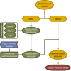 |
Fig. 1. Schematic flowchart of the galaxy-in-a-box model. The computation starts with generating the spatial (Sect. 2.2.1) and mass (Sect. 2.2.2) distributions of GMCs in the simulated galaxy. The GMC mass distribution serves as the input to the module generating the protostellar spatial, mass, and age distributions within individual star-forming clusters. Here, each randomly chosen GMC mass is an initial mass of the cluster. Having calculated these distributions, the model uses them to assign molecular outflow emission to each protostar within the cluster, based on the envelope mass–outflow intensity relation calculated using the Water Emission Database (Sect. 2.3). After repeating these calculations for all GMCs, the emission and mass of star-forming clusters are returned to the galaxy-in-a-box model. Subsequently, the model merges the spatial distribution of the initial GMCs with water emission emerging from the corresponding star-forming clusters. Once the model returns the expected emission from the galaxy, this raw galactic emission grid is convolved with a Gaussian beam, producing the integrated intensity image of the galaxy. In this flowchart yellow corresponds to the galactic part of the model (Sect. 2.2), green to the cluster model (Sect. 2.1), red to the last stage of the model, and blue to the external data input. |
2.1. Cluster-in-a-box model
Most stars form in clusters, especially in high-mass clusters (Lada & Lada 2003). These clusters harbor protostars covering the whole range of stellar masses. However, at the time of formation they are also deeply embedded in their natal clouds, and so it is impossible to access the initial main-sequence stellar populations forming within these clusters directly. Moreover, massive stars dominate cluster emission, making the low-mass population hard to access observationally. An alternative is to probe this population with outflow emission. Studies show that there is a proportionality between this emission and protostellar envelope mass (e.g., Bontemps et al. 1996; Skretas & Kristensen 2022). Kristensen & Bergin (2015) used this link to construct the cluster-in-a-box model1, simulating methanol emission from low-mass outflows in embedded star-forming clusters.
The cluster model consists of a template cluster and molecular emission assigned to each protostar in the cluster. The spatial distribution of protostars in the template cluster is based on the model by Adams et al. (2014), where the radial extent of the cluster can be described by the power-law function Rmax = R0(N/N0)αc, where N is the number of stars in the cluster and the power-law slope αc = 1/3. The age distribution of protostars in the stages Class 0, Class I, “flat-spectrum”, Class II, and Class III follows that of the Perseus low-mass star-forming cluster (Evans et al. 2009; Sadavoy et al. 2014). The model applies the Chabrier initial mass function (IMF; Chabrier 2003) for young clusters and disks. The outflow position angles are chosen randomly from 0° to 180°, as is the distance from the protostar to the outflow lobe with the maximum separation equal to 2 × 10⁴ AU. The molecular outflow emission is assigned based on a scaling relation of the observed outflow emission from single low-mass protostars in the nearby low-mass star-forming regions NGC 1333 and Serpens Main and their modeled envelope masses. However, the emission is assigned only to Class 0 and I protostars, because flat-spectrum, Class II, and Class III objects only produce negligible molecular outflows (Arce et al. 2007). The cluster-in-a-box model focuses on the 70 − 60 A+ methanol line at 338.409 GHz.
The cluster model did not include the contribution from high-mass sources, neither in the form of their outflows nor their hot cores. Nevertheless, a proof-of-concept study showed that the model reproduces the extended emission from a high-mass star-forming region to within a factor of two without tweaking the input parameters, suggesting that low-mass outflows account for ∼50% of the total cluster emission. These results indicate that a toy model of this kind can be used to constrain parameters of star-forming clusters and decipher the contribution from their components (i.e., molecular outflows and hot cores), and to reproduce their morphologies.
2.2. Galaxy-in-a-box
New telescope facilities, particularly ALMA, are now routinely observing molecular emission at high redshift (e.g., out to z ≳ 6, Strandet et al. 2017). One possibility for understanding the origin of this emission is to use Galactic star-forming clusters as templates of emission. This approach would consist first in scaling Galactic observations to cover entire galaxies, and then in comparing these scalings with actual observations of local galaxies. Next, the scalings would be extrapolated to the high-redshift regime (z ≳ 1), where they can be compared to observations. Practically, the approach would consist of first creating a cluster model (Sect. 2.1), then populating a galaxy with these model clusters, thereby going from a cluster-in-a-box model to a galaxy-in-a-box model. This model consists of a template (spiral) galaxy with molecular cloud spatial, age, and mass distributions, and of template stellar clusters with assigned outflow emission based on the cluster-in-a-box model. In this manner, emission from an entire galaxy can be simulated, with the advantage that the model only depends on a few input parameters.
Our knowledge of astrochemistry and star formation primarily comes from observations of the Milky Way (e.g., Herbst & van Dishoeck 2009). Thus, when first going to the extragalactic regime, the goal is to use the knowledge from the Milky Way together with a similar galaxy that could provide the pivotal information on its spatial structure. Furthermore, the galaxy should be nearby, well-studied, and ideally face-on, such that line-of-sight effects are minimized. One example of such a galaxy is the grand-design spiral Whirlpool Galaxy, M 51. In addition to the spiral structure, M 51 has an apparent size of 24 kpc (Jarrett et al. 2003), which is roughly comparable to the estimated size of the Galactic disk ≳30 kpc (Bland-Hawthorn & Gerhard 2016). It is nearby (D ∼ 7.6 Mpc; Ciardullo et al. 2002) and almost face-on (i ∼ 22°; Colombo et al. 2014a), making it an object of numerous studies, for example the Plateau de Bure Interferometer Arcsecond Whirlpool Survey (PAWS; Schinnerer et al. 2013). Therefore, in the following, we base the template galaxy against observational data from M 51.
For the galaxy-in-a-box we picked water as a default molecule for the simulation of galactic emission. The reason is that from the 30% of the molecular species observed in the Milky Way that were also detected in external galaxies (McGuire 2022), water stands out as a ubiquitous star formation tracer in the Milky Way with emission dominated by molecular outflows and is readily observed toward high-z galaxies (e.g., Yang et al. 2016, 2017; Jarugula et al. 2019; van Dishoeck et al. 2021). For the purpose of this work, we focused on the emission of the para-H2O 202 − 111 line at 987.927 GHz.
In addition to the change in the molecular species used to obtain the mass-intensity relation, the cluster model underwent a few upgrades while being adapted to the galactic model. One of the major changes is the spatial configuration defined in the cluster model. At a distance of ≥7.6 Mpc the structure of individual clusters is practically unresolvable (1″ corresponds to ∼40 pc). Therefore, the spatial component for the galactic model was discarded. Moreover, we used a novel distribution of protostellar ages following Kristensen & Dunham (2018). We describe all of the relevant changes and upgrades motivated by scaling up the cluster model in greater detail in the following paragraphs. First we describe the spatial distribution applied in the galaxy model (Sect. 2.2.1), then we define the molecular cloud mass distribution (Sect. 2.2.2), and from there we go to the age distribution (Sect. 2.2.3).
2.2.1. Spatial distribution
The spatial distribution of GMCs, in which young clusters form, in the galaxy-in-a-box model follows Ringermacher & Mead (2009):
 (1)
(1)
Here A is a scale parameter for the entire structure, while B and NS determine the spiral pitch. This formula assumes that all galaxies have “bars” hidden within a bulge. Increasing the N value results in tighter winding, and increasing B in greater arm sweep and smaller bars and/or bulge. To emulate M 51 we adopted the following values: A = 8.0, B = 1.0, and NS = 8.26. To obtain long spiral arms that wrap around each other, we chose an angle coverage ϕ of 500°. We also introduced a direct scaling parameter S = 1.5 to shift spiral arms closer together, toward the galaxy center, without altering their spatial setups. This is especially useful to simulate a central bulge within a galaxy. The parameter is designed to be added at the end of Eq. (1). The values were chosen to fit a galaxy with a ∼23 kpc diameter, which is roughly equivalent to the estimates of the M 51 spatial size (e.g., Jarrett et al. 2003). Figure 2 illustrates the quality of our fit.
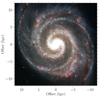 |
Fig. 2. Two-part spatial configuration used in the galaxy-in-a-box model mapped onto the image of M 51 from NASA’s Hubble Space Telescope (credit: NASA, ESA, S. Beckwith (STScI) and the Hubble Heritage Team (STScI/AURA)). The M 51 image was scaled to fit within the spatial size settings used in the model. The white squares represent the location of stellar clusters along the spiral arms. |
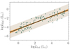 |
Fig. 3. Water line luminosity at 988 GHz vs. bolometric luminosity for objects from WED used in the simulations, with inclusion of a few additional sources that were excluded from the simulations due to lack of Menv data (San José-García 2015). The solid black line shows the best-fit proportionality, the orange filled region corresponds to the 95% confidence region of the correlation, and the shaded red region represents the region that contains 95% of the measurements. |
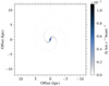 |
Fig. 4. Example integrated intensity map of the template galaxy with the standard setup. |
We built our radial distribution of stellar clusters by utilizing an exponential decline of stellar surface density Σstar with radius R as
 (2)
(2)
where hR is a characteristic scale-length. Here the exponential radial distribution corresponds to a probability density function for the location of stellar clusters along the spiral arms, which are then randomly located according to this function. We follow Casasola et al. (2017) and use the value hR = 2.38 pc in this study.
The density distribution of stars in M 51 resembles a skewed normal distribution (Scheepmaker et al. 2009). Therefore, the model initially assigns a given stellar cluster a randomly generated location along the spiral arm, and then a random position along the cross section of the spiral arm given by the skewed normal distribution. Studies show that the gas and dust density in galaxies typically decrease as a function of the radius from the center (e.g., Bianchi 2007; Hunt et al. 2015). Along with the stationary density wave predicting an age gradient across the arms, this decrease implies that star formation activity preferentially occurs in a narrowing band of the spiral arms. To simulate this effect, the standard deviation associated with the skewed normal distribution is scaled as a function of the distance from the center:
 (3)
(3)
This σ value was arbitrarily chosen based on a qualitative good fit with observations of star-forming regions in M 51 (Koda et al. 2011).
2.2.2. Molecular cloud mass distribution
In the galaxy-in-a-box model, the initial number of GMCs is specified and then each GMC is randomly assigned a mass following the molecular cloud mass distribution. The latter is described by the molecular cloud mass probability density function (PDF):
 (4)
(4)
We adopt a value of the slope, α = −1.64 following Roman-Duval et al. (2010). This value is in a good agreement with other Galactic studies of the GMCs, clouds, and clumps (e.g., Solomon et al. 1987; Urquhart et al. 2014). However, this power-law slope was derived for molecular clouds with masses between 105 M⊙ − 106 M⊙. Therefore, we assume that lower masses follow a similar slope and so we can use this α value for our study, where we utilize this relation for the mass range 104 M⊙ − 106 M⊙. Estimates of extragalactic α show that this value is probably not constant among galaxies, and there have been reports of variations reaching α ∼ −3.0 and estimates of the average α ∼ −2.0 (e.g., Rosolowsky 2005; Guszejnov et al. 2018; Mok et al. 2020). We evaluate the impact of different α values on the model in Sect. 3.1.
Subsequently, we use the mass distribution obtained with Eq. (4) to calculate the size of each molecular cloud. Here we follow the recent estimate of the mass–size relation for Galactic GMCs from Lada & Dame (2020):
 (5)
(5)
To account for the fact that not all of the molecular cloud mass is converted to stellar mass, we assign a star formation efficiency, εSF, to determine the total mass of the stellar population from the molecular cloud mass. In the model we apply εSF ∼ 10% for embedded clusters following Lada et al. (2010).
2.2.3. Age distribution
The characteristic timescale associated with star-forming regions is the free-fall timescale tff,
 (6)
(6)
where ρ is the density of the cluster calculated as the total mass of the progenitor molecular cloud divided by the volume of the cloud. The free-fall time reflects the time required for a medium with negligible pressure support to gravitationally collapse. Here, we utilize this timescale to determine a lifetime of the clusters. However, not all of the molecular reservoir will undergo gravitational collapse. Recent studies find that εSF per tff remains constant among different molecular clouds (e.g., Pokhrel et al. 2021). To account for this inefficiency and its influence on the efficiency of tff, we impose a scaling factor  . In this study we set the standard value of this factor to be 1. We also assume a constant free-fall time for the entire cluster.
To assign a random age to the cluster we scale tff with the chosen  , and subsequently choose random values ranging between 0 (newly formed) and 1 (completely collapsed). The assigned ages are used to calculate the star formation rate, given by
 (7)
(7)
where N(t) is the number of stars at time t, which is the current age of the cluster calculated from the free-fall time. Here, we make an assumption that λSF is constant for the entire cluster.
To assign the ages to protostars and determine their distributions within clusters, we follow Kristensen & Dunham (2018) and adopt a novel age distribution module. We start with the assumption that protostellar evolution is sequential, it begins at Class 0 and then goes through Class I, flat-spectrum, Class II, and ends at Class III. Then, with the constant star formation rate and protostellar half-lives, sequential decay is applied. This decay, associated with protostars going through the evolutionary stages, is characterized by the decay constant λD, where D represents the protostellar class. Values of λD for each evolutionary stage are estimated based on the observations of seven Galactic clouds (for further details, see Kristensen & Dunham 2018). With this, we calculate the fractional population of stars in each evolutionary class for all galactic clusters.
2.3. Water Emission Database
Our model relies on archival water observations. Thus, as a part of this project, we created the Water Emission Database (WED). The main goal of creating this database is to gather in one place all of the available water data, from both ground-based observatories and the Herschel Space Observatory, and to make it publicly available. This way the data serves the scientific community. The database is stored and maintained using the MySQL Database Service. However, access to the data is granted through regularly updated ASCII and CSV files available online and is independent of the database driver for safety measures.
Data from many Galactic surveys and observational projects are included in WED, for example Water In Star-forming regions with Herschel (WISH; van Dishoeck et al. 2011); the William Herschel Line Legacy Survey (WILL; Mottram et al. 2017); and Dust, Ice, and Gas in Time (DIGIT; Green et al. 2013). Ultimately, the database will also include extragalactic observations of water emission. The values that we store are particularly useful for this study. For example, we focused on water fluxes and parameters describing source properties. This means that we not only store the values from specific studies, but we also keep a unified system of parameters important to characterize the sources. Currently, WED covers 79 observed water transitions up to the para-H2O 919 − 808 transition at 5280.73 GHz (56.77 μm). Emitting sources at these transitions include the whole range of Galactic protostellar sources, with the majority of low-mass protostars.
The database holds the data in tables arranged in 20 columns (see Table 2) and shares them in the form of CSV and ASCII files available online on the project website2. All of the files that are available for download are fully described and updated whenever there is a change in the database. The galaxy-in-a-box model downloads the data directly from the website, which makes access to the model completely independent from the restricted MySQL server.
For the purpose of this work, we use a very particular subset of WED. We chose the data for the para-H2O 202 − 111 line at 987.927 GHz. This water line is among the brightest H2O transitions observed toward Galactic star-forming regions. Furthermore, it is not a ground-state transition, and so it only mildly suffers from self-absorption even toward high-mass objects (van der Tak et al. 2013). Finally, this transition is routinely observed toward extragalactic and even high-z objects (e.g., Yang et al. 2016, 2017; Jarugula et al. 2019). The data available in WED for this particular line cover the whole range of sources, and therefore gives a broad overview of water emission. San José-García et al. (2016) identified an intensity–envelope mass relation for this line, log LH2O = ( − 2.91 ± 0.10)+(1.19 ± 0.05)⋅log Menv, which we also observe for the data used in this study (see Fig. 5). As mentioned, the emission assignment utilizes the relationship between the line intensity and envelope mass. At first, Class 0 and Class I objects are assigned with a stellar mass sampled from the IMF. Then we subsequently convert the stellar masses to envelope masses by assuming the envelope mass corresponds to 3× and 1.5× stellar mass for Class 0 and I protostars, respectively (e.g., André et al. 2010, and for a more in-depth discussion Offner et al. 2014). Following this, by using the intensity–envelope mass relation, we assign outflow emission to these deeply embedded protostars. We build this relation for the para-H2O 202 − 111 line data from the WISH and WILL samples. The observed intensities are distance-normalized to get a distance-independent measurement. To assess the goodness of fit of the correlation in our regression model, we examined its R-squared value, which in this case corresponds to 89%, indicating a strong relationship between envelope mass and intensity. We derived the correlation as
 (8)
(8)
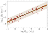 |
Fig. 5. Water emission at 998 GHz vs. envelope mass (Menv) for objects from WED used in the simulations. Colors as in Fig. 3. |
where the intensity is normalized to the distance of M 51 (i.e., 7.6 Mpc). From the above correlation we see that there is a near-proportionality between Iν and Menv, Iν ∝ Menv.
3. Results
With the default galactic and star formation parameters described in Sect. 2.2 and gathered in Table 1, we obtain an integrated intensity map of the desired molecular emission, as well as mass, total emitted emission, and number of stars of each star-forming cluster within the simulated galaxy. An example integrated intensity map for the model with default parameters is presented in Fig. 4. With the chosen spatial setup, most of the emission comes from the innermost parts of the galaxy where the bulge is located, and here individual clusters are not resolved with the applied beam size of  (see Table 1). The farther from the bulge, the lower the emission and the easier it is to resolve clusters within spiral arms, although the surface brightness of course also decreases.
Overview of the most important global parameters in the galaxy-in-a-box model.
Description of WED table columns.
To explore the impact of the global star formation parameters on the expected emission from clusters in a simulated galaxy as well as the galaxy itself, we conducted a parameter-space study. The changes in parameters were set with respect to the standard model configuration (Table 1). We focused on the variations caused by the most important global SF-related parameters: (i) α, describing the slope of molecular cloud mass distribution; (ii) εSF, the star formation efficiency per free-fall time; (iii)  , the free-fall scaling parameters; and (iv) the power-law slope for the high-mass end of IMF. For each change in parameters, we run ten simulations to derive the average of the predicted emission, while for the standard setup we decided on 30 model runs to lower the variations in the derived values. The choice of running ten simulations was motivated by cutting down on the computational time, and it is enough to show the variability in the model outcomes. We explored the cumulative impact of these parameters on the total galactic emission, radial profiles of the emission maps, and distributions of emitted flux by the galactic clusters. As we show below, these seem to be consistently skewed. Therefore, we chose median values as a measure of central tendency and explored the spread of these distributions with the interquartile range method (IQR or midspread), providing information on the middle 50% of values with the median being in the center of the range.
3.1. Molecular cloud mass distributions
The standard value of α is set to −1.64 (Roman-Duval et al. 2010). Different studies report a spread in α depending on the studied regions (e.g., Solomon et al. 1987; Rosolowsky 2005; Mok et al. 2020), and following these studies we explore the change in expected emission for α = −1.5, −2, and −2.9. The highest α follows the steepest index reported by Rosolowsky (2005). To investigate this impact we compared the distributions of flux emitted by the clusters and radial profiles of galactic emission.
We observe no apparent variations in the expected emission caused by the change in α. It is true both for the flux distributions and for the mean radial profiles Fig. 6. However, looking at the values obtained for the molecular cloud mass distribution (see Table 3) we see a clear trend, indicating that with increasing α, the median flux, the total galactic emission, and the interquartile range increase. This result is consistent with the nature of the corresponding mass distributions as the steeper the slope, the more emission comes from low-mass clusters, which in turn lowers the total observed emission.
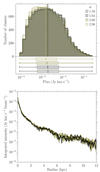 |
Fig. 6. Results of multiple model runs with varying power-law slopes α of molecular cloud mass distributions. Top: distributions of cluster emission derived for simulations with different power-law slopes α of molecular cloud mass distributions. The vertical dashed lines correspond to the median flux of each distribution. In the bottom box plot the interquartile ranges are presented. The notches in the boxes indicate the 95% confidence intervals around the median. The whiskers spread to the beginning (0%) and the end (100%) of the distributions. These are the mean distributions from a series of ten simulations for each varying parameter. Bottom: radial profiles of emission from the galaxies of the corresponding α values. The radial profiles were calculated from the center of the galaxy all the way to its outskirts. The solid lines correspond to the mean profiles derived from ten simulations, while the shaded regions represent the spread of the mean values based on their standard deviations. |
Simulation results for different molecular cloud mass distributions.
3.2. Initial mass function
In the model we adopted three types of IMF based on the Chabrier (2003) IMF form for young clusters and disk stars. By introducing changes in the slope of the high-mass end of the IMF (x), which applies to stars with M⋆ > 1 M⊙, we defined bottom-heavy and top-heavy forms. With the standard value of x = −2.3, the slope for the bottom-heavy IMF is defined as x − 1, while for the top-heavy it is x + 1. This is a purely empirical parameterization, although it is in reasonable agreement with studies reporting x values for bottom-heavy and top-heavy IMF forms (for a recent review, see Smith 2020).
There is no apparent difference in the examined values for any of the IMF types (see Table 4), although it is clear that our top-heavy IMF model tends to produce slightly more emission than the bottom-heavy model. We discuss this further in Sect. 4. The lack of dominance of any IMF type is also true for the mean radial profiles of galaxies depicted in Fig. 7. Here, we see that neither around the inner part of spiral arms nor around their outer parts do any of the considered IMF types take over the emission, and the radial profiles are indistinguishable.
Simulation results for different IMF configurations
3.3. Star formation efficiencies
We probed the impact of εSF on emission outputs by varying its values from 1% to 30%. The outputs vary strongly between different εSF values with a clear trend of increasing flux with εSF, as seen in Fig. 8. The difference between the highest and the lowest values roughly corresponds to one order of magnitude for all of the considered values. Moreover, we see that the shape of the distribution does not vary significantly across different εSF values; instead, higher εSF merely translates distributions to higher flux values. This way, for the lowest εSF = 1% we derived the total galactic emission of 6.96 Jy km s−1, while one order of magnitude higher εSF = 10% results in an increase in the same parameter of approximately one order of magnitude, giving 7.02 × 101 Jy km s−1. In addition to the total galactic emission Itot, this trend holds for the median fluxes  , and for the midspreads, and it is clear that the multiplication of εSF on average corresponds to the same multiplication of flux (see Table 5).
Simulation results for different star formation efficiencies.
From mean radial profiles (see Fig. 8) it is also clear that the increase in the εSF value results in a subsequent increase in average emission from the galaxy. Here the highest differences in intensities are also around one order of magnitude. Therefore, the higher the εSF, the more emission comes from spiral arms at different points of the radius. In addition, for εSF = 1% and εSF = 3%, the drop in emission in the outermost parts of the galaxy results in higher variations and a more significant drop in the observed emission.
3.4. Free-fall-time scaling
We studied the impact of the free-fall time in the form of  by adopting values ranging from
  to
to  . The scaling factor introduced in this study represents how many free-fall times it takes to form most of the stellar population in a single cluster and relates to the free-fall time efficiency as
  , following Da Rio et al. (2014), where they estimated the time required to form 90% of stars in the cluster. Therefore, with this choice of the
  values, we evaluate the impact of the free-fall time efficiencies spreading over one order of magnitude, between ϵff ∼ 0.01 − 0.1.
We observe a very distinct relation between emitted flux and  values, namely that with decreasing
  the observed total flux increases. Moreover, decreasing
  is associated with condensation of flux distributions, which get both narrower and flatter, and are shifted toward higher flux values (see Fig. 9). The lowest
  results in a median flux value that is one order of magnitude higher than that derived for the highest
  (see Table 6). In addition, the beginnings of each distribution are shifted by one order of magnitude from ∼10−5 to ∼10−4 Jy km s−1 for the highest and lowest
  , respectively.

Simulation results for different free-fall time scaling factors.
From the radially averaged flux from galaxies with different  we see a trend similar to that for varying εSF values. The flux profile from different model outcomes divides into distinguishable pairs for
  and
and  , although the differences stop being prominent at the galactic outskirts where the flux is the weakest. Here, in particular, the profiles for
  and 5 get blended and cause major fluctuations of more than two orders of magnitude in the observed flux.
3.5. Total galaxy emission
We calculated the integrated galactic emission for model outcomes with varying parameters (Fig. 10). The total integrated flux Itot was calculated from the mean flux distributions, and for the standard setup it is equal to 7.02 × 101 Jy km s−1.
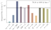 |
Fig. 10. Total galactic emissions derived from all of the clusters averaged over ten simulations for each setup. The dashed black horizontal line corresponds to the standard setup described in Table 1. |
From Fig. 10 we see that only two Itot-values significantly exceed the default model outcome. The highest value of Itot is observed for simulations with εSF = 30% and is equal to Itot = 2.11 × 10² Jy km s−1. The second highest value comes from the setup with  with 1.12 × 10² Jy km s−1. For the varying α the highest total emission is derived for α = −1.5 and falls almost at the same level as the output from the standard model. A similar thing happens for the top-heavy IMF, which exceeds the default Itot by 1.56 × 101 Jy km s−1.
The most visible changes are for the outputs that fall below the standard threshold. Here we observe that the lowest total emission output is derived for the setup with the lowest εSF resulting in a one order of magnitude drop in Itot = 6.96 Jy km s−1. Subsequently, the second lowest value is a result of setting  to 5.0 with Itot = 1.91 × 101 Jy km s−1. However, the second lowest value of εSF results in a very similar result with Itot = 2.10 × 101 Jy km s−1. Therefore, these two parameters have the biggest impact on emission and show the highest spread in derived Itot values, while the lowest impact is observed for changes introduced to the molecular cloud mass distribution with the α index.
4. Discussion
In the following we discuss model outcomes and their possible explanations. We also evaluate the impact of different star formation parameters and compare the joint effect of the most influential ones. Moreover, we focus on addressing the question of what other star formation-associated processes, not incorporated into the current version of the galaxy-in-a-box model, could influence the results. Finally, we explore the implications of this proof-of-concept study for observations.
4.1. Varying molecular cloud mass distributions
Molecular cloud mass distributions are usually described by a single power-law function (Eq. (4)). Some studies (e.g., McKee & Williams 1997; Rosolowsky 2005) propose truncated power-law distributions. However, when the truncated distribution applies, the cut-off point usually lies outside the mass range considered in this study (i.e., for MGMC > 106 M⊙). The mass distribution can be expressed either in differential form, as in this work, or in cumulative form with α > −1 (Heyer & Dame 2015). Many Galactic surveys report α > −2 (e.g., Solomon et al. 1987; Roman-Duval et al. 2010; Urquhart et al. 2014), while even steeper distributions are found in the outer parts of the Milky Way and in extragalactic regions, with −2.9 < α ≤ −2 (e.g., Rosolowsky 2005; Guszejnov et al. 2018; Mok et al. 2020). The α index indicates whether most of the mass is contained in high-mass (α > −2) or low-mass clouds (α < −2).
We evaluated the impact of α on the predicted emission. It appears that steeper distributions result in lower medians and lower total fluxes (see Figs. 6 and 10). For the standard setup with α = −1.64, we see a clear difference when comparing these outcomes to α = −2.9. For these, the median values differ by 3.44 × 10⁻⁴ Jy km s−1, where the IQRs are narrower by 1.17 × 10⁻³ Jy km s−1 for α = −2.9. This small yet potentially observable level of discrepancy means that the model could distinguish the molecular cloud distributions for slopes with a difference on the order of ∼1.
This effect of lowered values with increasing steepness of the mass distribution is somewhat expected. Steeper distributions result in a greater number of molecular clouds with lower masses and produce smaller star-forming clusters. The greater number of low-mass clusters in turn emit less and thus lower total galactic emission, and this is what we see in Fig. 6.
Comparing the impact of molecular cloud mass distribution and IMF, as these two seem to have the smallest impact on the predicted emission, we see that the standard and bottom-heavy IMFs result in median fluxes similar to molecular cloud mass distributions with α ≥ −2. However, the most bottom-heavy form of the molecular cloud mass distribution stands out, similarly to the top-heavy IMF. Therefore, when conducting observational comparisons to model outputs, putting constraints on the slope of α, at least for its most varying values, or IMF shape, may be required to fine-tune the model and obtain better agreement with the observations.
4.2. IMF constraints
The parameterization of the IMF varies between studies, where the used format and high-mass cutoff differs between objects and redshifts (e.g., Chabrier 2003; Hoversten & Glazebrook 2008; van Dokkum 2008; Smith 2020); the standard form is as follows: N(M)dM ∝ M−2.35 (Salpeter 1955). For more bottom-heavy IMF parameterizations, more low-mass stars are formed, while more top-heavy distributions lead to the presence of more high-mass stars.
In this study we followed a widely used form of the IMF, the Chabrier IMF (Chabrier 2003), and adjusted it so it roughly represents the three main functional forms: standard, bottom-heavy, and top-heavy. As the building blocks of our model are molecular clouds from which individual star-forming clusters form, the IMF directly influenced the stellar mass distribution of each cluster and emission component. By studying variations on these local building blocks and large galactic scales, we see no significant variations imposed by the different IMF forms. However, for the standard IMF we see that the top-heavy distribution results in a slight increase in emission, while the opposite happens after adopting the bottom-heavy distribution. This result is expected. On the one hand, low-mass protostars dominate star formation in total mass and number (Kroupa 2001). The size of this population is increased or decreased for the bottom- and top-heavy IMFs, respectively. On the other hand, high-mass protostars are far more energetic than low-mass ones. Moreover, with  water is a low-contrast mass tracer. Hence, the more massive the envelope, the higher the emission.
When comparing results obtained for different IMF forms, we also see that the total flux obtained for the bottom-heavy IMF is very similar to that derived for the standard IMF. These two are also very similar when we consider their flux distributions and radial profiles as seen in Fig. 7. The same for their IQRs. Therefore, the model cannot distinguish these from one another. The top-heavy IMF, on the other hand, seems to differ when it comes to the IQR and the range spanned by the flux distribution. However, the variation is in the range of 5.73 − 7.87 × 10⁻³ Jy km s−1 for IQR and only 1.81 − 2.51 × 10⁻³ Jy km s−1 for  . Nevertheless, this is the only IMF form that could be necessary to fine-tune the model when comparing it with observations.
Looking at the total flux plot in Fig. 10 we see that the output for the standard and bottom-heavy IMFs is comparable to other outputs derived for molecular cloud mass distributions for which α was set to −1.5 and 2.0. The only difference between these setups can be seen in the shapes of their radial profiles; however, this may be not significant enough to distinguish these distributions from each other.
4.3. Effect of star formation efficiency
The star formation efficiency describes the amount of molecular gas that ends up in stars. The increase in εSF directly translates to an increase in the number of (proto)stars, which results in more emission from clusters. Different values of εSF are reported toward different types of sources across cosmic time, varying from 3% in nearby molecular clouds to 30% in Galactic embedded clusters (Lada & Lada 2003) and extragalactic GMCs (Dessauges-Zavadsky et al. 2019). In this work, the impact of εSF > 30% is not evaluated, as εSF is closely related to the gas depletion time, and with higher εSF molecular gas is used at a higher rate and is sustained for a shorter time.
Analyzing the impact of εSF on the expected emission locally and on a galactic scale, we observe a clear and systematic increase in emission with increasing εSF. The observed increase in emission is roughly proportional to the increase in εSF. There is a shift of the flux distributions as seen in Fig. 8. The IQRs follow the same trend, and are in the range ∼6 × 10⁻⁴ − 2.0 × 10⁻² Jy km s−1. This suggests that the model can be used to distinguish different values of εSF, at least when no other parameter varies.
Distributions drawn from model outputs with varying εSF show significant variations when considering all of the analysis, which is also true for the impact of  . However, these two parameters significantly differ when it comes to the shape of the flux distributions and radial profiles. Therefore, it should be possible to evaluate which parameter could explain the observed galactic emission.
4.4. Influence of the free-fall time scaling factor
The last considered parameter is the free-fall time scaling factor  . Here we arbitrarily chose all of the values to explore how altering the ages of clusters could affect the expected emission. With
  we effectively lower the ages of protostars within the cluster, and therefore increase the contribution from Classes 0 and I. Therefore, with lower
  values we would expect higher emission both globally and locally.
From the flux distributions and radial profiles in Fig. 9 we see that there is indeed an increase in flux with the decrease in  . Moreover, all of the distributions tend to flatten with this decrease. We also observe a peculiar shape of the distribution derived for the smallest
  . The possible explanation for this peculiar shape is that such a huge change in free-fall time results in constraints on the age distribution of clusters within galaxies. It is also the distribution with the higher median, which indicates a greater number of Class 0 sources within clusters, which produce more molecular emission from outflows.
Following Kristensen & Dunham (2018), the fraction of Class 0/I cores decreases with the age of the cloud and reaches a steady state at ∼0.5 Myr. Therefore, as the scaling of the free-fall time increases, especially when  , clusters more accurately represent the dynamics of stellar formation. This in turn results in a greater range of flux distributions and lower median fluxes, as the fraction of Class 0/I cores decreases.
The outcome for  is similar to that for εSF = 3%, when considering the cumulative galactic flux shown in Fig. 10. Nevertheless, the difference between these outputs is potentially observable, especially that
  gives a flatter flux distribution. Therefore, the model could distinguish the emission for these global parameters.
4.5. Interplay of the most influential parameters
The most influential parameters in the model are  and εSF. Thus, to understand and explore the combined effect of these parameters on simulated galaxies we ran the model for all of the possible combinations of the values considered in this study. Then we evaluated the outcomes of these simulations by calculating the distributions of cluster fluxes and their corresponding midspreads (see Fig. 11) and galactic radial profiles (Fig. 12). Moreover, we color-coded the results of each simulation based on the integrated intensities of the flux distribution. The heat map with corresponding integrated fluxes is presented in Appendix A.
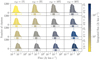 |
Fig. 11. Distributions of cluster emission derived for simulations with varying free-fall time scaling factor |


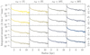 |
Fig. 12. Radial profiles of emission from the same set of simulations and color-coding as in Fig. 11. The solid lines correspond to the mean radial profile, while the shaded regions represent the variability of each profile, based on the standard deviation of each profile. |
The distribution of fluxes changes according to what we observed when studying the impact of  and εSF separately, namely that median flux and integrated intensity within galaxies increases with increasing εSF and decreasing
  . Interestingly, εSF seems to mainly influence the median flux by shifting the distribution toward higher flux values proportionally to the magnitude of the increase. In addition, the shift is not associated with any significant changes in the shape of the distributions. On the other hand,
  increases the median fluxes, but does not shift the whole distribution. With the decrease in
  the distributions flatten and, based on the midspreads, the high-flux tail seems to catch up with the rest of the distribution. Subsequently, there is a decrease in the spread of observed flux values. The lower-flux part of the distribution shifts toward higher flux values, but it does not affect the highest flux values.
The changes observed on galactic scales also reveal complex outcomes of the interplay of these parameters. Here we observe that εSF basically scales the radial profiles up and increases the level of each emission point, especially in the inner galaxy where most of the clusters reside. It also influences the visibility of the spiral arm bumps in the radial profiles. Surprisingly, these bumps are more prominent with the increase in the free-fall time scaling factor. However, this change is also associated with the increased radial profile variability.
By looking at the simulations obtained for all of the available combinations, we see that the impact of each parameter is different, and the only common characteristic is a strong influence on the observed emission. From the flux distributions we find that for spatially resolved observations the possible value of each parameter can be estimated because these parameters introduce very distinct features to the shape and properties of each distribution, while in the case of unresolved observations these values can be determined from the features seen in the galactic radial profiles. Therefore, our model can be used to reveal these global star formation parameters or at least indicate which one has the prevalence in increased or decreased star formation activity in a galaxy.
4.6. Other effects
Other factors could play a role in water excitation. These include the local and global effects of star formation processes and galactic evolution and structure.
The warm (≳100 K) and dense (≳106 cm−3) inner regions of protostars, known as hot cores, exhibit conditions that support the presence of a rich chemistry (Herbst & van Dishoeck 2009). Under these conditions all water ice should sublimate, and the observed gaseous water abundances should match the expected water ice abundances. However, the observations do not follow these expectations, showing that most of the observed gaseous water is universally associated with warm outflowing and shocked gas, with a negligible contribution from hot cores (van Dishoeck et al. 2021). The low surface brightness of the hot cores along with the high dust opacity at 1 THz obscuring the hot cores makes them practically invisible in a Herschel beam (Visser et al. 2013; Herpin et al. 2012).
On larger scales the question arises of the emission from molecular clouds themselves. Here, water vapor is generally not detected in the Milky Way (e.g., Dionatos et al. 2020). The only noteworthy exception are the regions exposed to enhanced UV radiation, the so-called photon dominated regions with one narrow emission component (Bjerkeli et al. 2012). However, the overall molecular cloud contribution to the observed water emission is insignificant for the results of this study, particularly for the higher-excited 202 − 111 transition. Taking a global view of galaxies, active galactic nuclei (AGNs) could play a role in increasing or decreasing water emission, both locally and globally. Studies report quenching of star formation in AGN host galaxies, which would lower the number of protostars and thus outflows (e.g., Fabian 2012; King & Pounds 2015; van Dishoeck et al. 2021, and references therein). Moreover, AGNs can produce conditions favoring molecular excitation or dissociation if the radiation becomes too strong. The exact influence of the AGN feedback on water excitation is not well understood, but it appears that the presence of AGNs has little impact on the excitation of the water line considered in this study, the para-H2O 202 − 111 line at 987.927 GHz. Specifically, Jarugula et al. (2019) spatially resolved H2O emission in this transition toward the Cloverleaf quasar, which is a strongly lensed AGN, at a resolution of 1 kpc, but found no trend with distance to the actual AGN. Thus, considering AGN feedback would likely have a negligible effect on the results of this study.
4.7. Implications for observations
Verification of the model can only be obtained by benchmarking its outcomes against observations. Ideally, these observations should spatially resolve individual star-forming clusters. This way, the cluster flux distribution is compared with a simulated galaxy. To come down to ∼10 pc scales and spatially resolve the whole range of molecular cloud sizes, the resolution should be on the order of  at 7.6 Mpc.
The results presented from our proof-of-concept study are for a resolution of  , which at 7.6 Mpc corresponds to ∼70 pc. This resolution is comparable to the resolution at which M 51 was observed as part of the PAWS program (Schinnerer et al. 2013), and where individual GMCs are resolved. Therefore, smaller clouds are unresolved in the galactic image. However, only a handful of high-redshift star-forming galaxies are spatially resolved in H2O emission, although at ∼1 kpc scales (Jarugula et al. 2019). Most observations do not resolve emission, and comparisons would have to be made based on the total fluxes or water line luminosities rather than on radial profiles or the shape of cluster flux distributions. With this assumption, we can make a tentative comparison of water line luminosities observed toward nearby and distant galaxies with the values derived in this study.
The average total flux of ∼70 Jy km s−1, corresponding to ∼1300 L⊙, derived for the simulated galaxies in this study remains approximately one order of magnitude below the luminosity derived for the nearby starburst M 82 (Yang et al. 2013), where the star formation rate (SFR) is approximately one order of magnitude higher (e.g., de Grijs et al. 2001) than the Milky Way or M 51. The observed luminosities toward several luminous infrared galaxies (LIRGs) and ultra-luminous infrared galaxies (ULIRGs) at larger distances (Yang et al. 2013) or high-z starbursts at z ∼ 2 − 4 (e.g., van der Werf et al. 2011; Omont et al. 2011, 2013; Yang et al. 2016; Jarugula et al. 2019) remain up to ∼2 − 4 orders of magnitude higher. However, this difference is expected and consistent with the increasing SFRs of these galaxies, especially when considering the high-z galaxies where SFRs often exceed ∼1000 M⊙ yr−1, which naturally boosts star formation, and hence the emission coming from the protostellar outflows. However, more comparisons are needed to fully assess the differences between the model and high-redshift observations, but this is beyond the scope of this paper.
There are several ways in which to interpret the difference between the model outcomes and the observations of high-z galaxies. First of all, our template galaxy resembles the nearby M 51 galaxy. We chose this particular galaxy instead of a well-studied high-redshift galaxy because we wanted to start with an object with a known molecular cloud distribution (e.g., Hughes et al. 2013; Colombo et al. 2014b) as this is one of the building blocks in our model. Second, our results are for a standard IMF (Lada & Lada 2003); there are indications that IMFs toward high-z galaxies are significantly more top-heavy than those we tested here, which would serve to further boost emission from the high-mass stars. However, this in turn implies that we are dealing with a different spatial setup, galactic size, and internal galactic environment. This size difference is very prominent, as spatially resolved high-redshift galaxies have radii in the range of 0.95 − 2.24 kpc (Jarugula et al. 2019), while M 51 has a radius of ∼12 kpc.
On the other hand, there is reasonable agreement between the model results and observations of galaxies that lie closer to M 51. Sandqvist et al. (2021) reported water flux measurements from the Herschel SPIRE observations toward the NGC 1365 galaxy, lying at a distance of 18.6 Mpc (Madore et al. 1998). The observed flux corresponds to 3081.9 Jy km s−1, which falls on the higher end of the fluxes derived for the model results when distance-corrected, and corrected for the SFR in NGC 1365 being approximately one order of magnitude higher than that of the Milky Way and M 51. For a nearby starburst, Mrk 231 at a distance of ∼200 Mpc (van der Werf et al. 2010), Omont et al. (2011) reports a flux of 718 Jy km s−1, which is distance- and SFR-corrected, and also falls at the high end of the simulated fluxes.
It is clear that both the star formation efficiency and the free-fall scaling parameter can affect the H2O flux dramatically (e.g., Fig. 11). A single integrated H2O flux is not going to constrain either parameter, and additional constraints are needed. To constrain the star formation efficiency, for example, the total number of stars formed combined with the amount of molecular material available should be observed. The former is best constrained through an in-depth look into stellar masses in galaxies, both nearby and at high-redshift. One way to do this is through near- and mid-IR observations, where the James Webb Space Telescope (JWST) will provide a great advance, especially for the high-redshift regime. The molecular material available can be probed either through low-J CO emission or dust emission. Although there are known problems with both tracers (e.g., Pitts & Barnes 2021), they are the best tracers at the moment for the total gas mass. Thus, with the combination of JWST observations of the stellar mass and, for example, ALMA observations of the total gas mass, the star formation efficiency can be independently constrained.
Another factor to consider is the detailed comparisons of spatially resolved observations with model results, where it would be possible to evaluate which sets of star formation parameters can reproduce the galactic emission. Here, for example, by analyzing the flux distribution of the observed emission (similar to Fig. 11), it would be possible to put constraints on these parameters and pinpoint their most probable values.
5. Conclusions
We created a galactic model of emission that could arise from active galactic star-forming regions. In this paper we demonstrated the main principles behind the galaxy-in-a-box model and explored how it can serve as a tool to study and better understand star formation activity in galaxies even at high redshift. For a template galaxy set to resemble the grand-design spiral Whirlpool Galaxy M 51, we evaluated the impact of important global star formation parameters on model results. We conducted this parameter space study for the para-H2O 202 − 111 line at 987.927 GHz. The main results are as follows:
-
Emission from the para-H2O 202 − 111 line is a low-contrast tracer of active star formation with ∫Iν ∝ Menv;
-
The initial mass function along with molecular cloud mass distribution have little impact on predicted water emission;
-
An increase and decrease in star formation efficiency εSF will respectively increase and decrease the predicted emission, both locally and globally;
-
With the decrease in free-fall time scaling factor
 we observe a corresponding increase in galactic emission and flattening of star-forming flux distribution, which indicates increasing populations of Class 0 and Class I protostars;
 -
At the moment, further constraints are needed to break model degeneracies; these additional constraints include JWST observations combined with low-J CO observations, and resolved observations of H2O emission.
A tentative comparison of model outcomes with observational data for high-redshift galaxies yields realistic results and opens new paths to improve the model, so it can become a reliable proxy to reveal star formation in galaxies throughout cosmological times. In the near future we plan to introduce the possibility of turning on or off AGN feedback and to conduct detailed comparisons of model results with observations of local and distant LIRGs, ULIRGs, and HyLiRGs (Hyper-Luminous InfraRed Galaxies). Furthermore, since our model is not designed specifically for water molecules, we intend to explore the results for other unique outflow tracers, like high-J CO (J ≥ 10). It will be important to constrain which global star formation parameters that have not impacted our results for water emission will behave differently for other molecular tracers.
The codes required for running the model are publicly available at https://github.com/egstrom/cluster-in-a-box
Acknowledgments
The research of KMD and LEK is supported by a research grant (19127) from VILLUM FONDEN. This article has been supported by the Polish National Agency for Academic Exchange under Grant No. PPI/APM/2018/1/00036/U/001.
References
- Adams, F. C., Fatuzzo, M., & Holden, L. 2014, ApJ, 789, 86 [NASA ADS] [CrossRef] [Google Scholar]
- André, P., Men’shchikov, A., Bontemps, S., et al. 2010, A&A, 518, L102 [NASA ADS] [CrossRef] [EDP Sciences] [Google Scholar]
- Arce, H. G., Shepherd, D., Gueth, F., et al. 2007, in Protostars and Planets V, eds. B. Reipurth, D. Jewitt, & K. Keil, 245 [Google Scholar]
- Bally, J. 2016, ARA&A, 54, 491 [Google Scholar]
- Bianchi, S. 2007, A&A, 471, 765 [NASA ADS] [CrossRef] [EDP Sciences] [Google Scholar]
- Bisschop, S. E., Jørgensen, J. K., van Dishoeck, E. F., & de Wachter, E. B. M. 2007, A&A, 465, 913 [NASA ADS] [CrossRef] [EDP Sciences] [Google Scholar]
- Bjerkeli, P., Liseau, R., Larsson, B., et al. 2012, A&A, 546, A29 [NASA ADS] [CrossRef] [EDP Sciences] [Google Scholar]
- Bland-Hawthorn, J., & Gerhard, O. 2016, ARA&A, 54, 529 [Google Scholar]
- Bontemps, S., Andre, P., Terebey, S., & Cabrit, S. 1996, A&A, 311, 858 [NASA ADS] [Google Scholar]
- Casasola, V., Cassarà, L. P., Bianchi, S., et al. 2017, A&A, 605, A18 [NASA ADS] [CrossRef] [EDP Sciences] [Google Scholar]
- Chabrier, G. 2003, PASP, 115, 763 [Google Scholar]
- Ciardullo, R., Feldmeier, J. J., Jacoby, G. H., et al. 2002, ApJ, 577, 31 [Google Scholar]
- Colombo, D., Meidt, S. E., Schinnerer, E., et al. 2014a, ApJ, 784, 4 [Google Scholar]
- Colombo, D., Hughes, A., Schinnerer, E., et al. 2014b, ApJ, 784, 3 [NASA ADS] [CrossRef] [Google Scholar]
- Da Rio, N., Tan, J. C., & Jaehnig, K. 2014, ApJ, 795, 55 [NASA ADS] [CrossRef] [Google Scholar]
- de Grijs, R., O’Connell, R. W., & Gallagher, J. S., III 2001, AJ, 121, 768 [NASA ADS] [CrossRef] [Google Scholar]
- Dessauges-Zavadsky, M., Richard, J., Combes, F., et al. 2019, Nat. Astron., 3, 1115 [NASA ADS] [CrossRef] [Google Scholar]
- Dionatos, O., Kristensen, L. E., Tafalla, M., Güdel, M., & Persson, M. 2020, A&A, 641, A36 [NASA ADS] [CrossRef] [EDP Sciences] [Google Scholar]
- Evans, N. J., II, Dunham, M. M., Jørgensen, J. K., et al. 2009, ApJS, 181, 321 [Google Scholar]
- Fabian, A. C. 2012, ARA&A, 50, 455 [Google Scholar]
- Fraser, H. J., Collings, M. P., McCoustra, M. R. S., & Williams, D. A. 2001, MNRAS, 327, 1165 [Google Scholar]
- González-Alfonso, E., Smith, H. A., Ashby, M. L. N., et al. 2008, ApJ, 675, 303 [CrossRef] [Google Scholar]
- González-Alfonso, E., Fischer, J., Aalto, S., & Falstad, N. 2014, A&A, 567, A91 [NASA ADS] [CrossRef] [EDP Sciences] [Google Scholar]
- Green, J. D., Evans, N. J., II, Jørgensen, J. K., et al. 2013, ApJ, 770, 123 [Google Scholar]
- Guszejnov, D., Hopkins, P. F., & Grudić, M. Y. 2018, MNRAS, 477, 5139 [NASA ADS] [CrossRef] [Google Scholar]
- Herbst, E., & van Dishoeck, E. F. 2009, ARA&A, 47, 427 [NASA ADS] [CrossRef] [Google Scholar]
- Herpin, F., Chavarría, L., van der Tak, F., et al. 2012, A&A, 542, A76 [NASA ADS] [CrossRef] [EDP Sciences] [Google Scholar]
- Heyer, M., & Dame, T. M. 2015, ARA&A, 53, 583 [Google Scholar]
- Hodge, J. A., & da Cunha, E. 2020, R. Soc. Open Sci., 7, 200556 [NASA ADS] [CrossRef] [Google Scholar]
- Hollenbach, D., Kaufman, M. J., Bergin, E. A., & Melnick, G. J. 2009, ApJ, 690, 1497 [NASA ADS] [CrossRef] [Google Scholar]
- Hoversten, E. A., & Glazebrook, K. 2008, ApJ, 675, 163 [Google Scholar]
- Hughes, A., Meidt, S. E., Colombo, D., et al. 2013, ApJ, 779, 46 [NASA ADS] [CrossRef] [Google Scholar]
- Hunt, L. K., Draine, B. T., Bianchi, S., et al. 2015, A&A, 576, A33 [NASA ADS] [CrossRef] [EDP Sciences] [Google Scholar]
- Jarrett, T. H., Chester, T., Cutri, R., Schneider, S. E., & Huchra, J. P. 2003, AJ, 125, 525 [Google Scholar]
- Jarugula, S., Vieira, J. D., Spilker, J. S., et al. 2019, ApJ, 880, 92 [Google Scholar]
- Jørgensen, J. K., Belloche, A., & Garrod, R. T. 2020, ARA&A, 58, 727 [Google Scholar]
- King, A., & Pounds, K. 2015, ARA&A, 53, 115 [NASA ADS] [CrossRef] [Google Scholar]
- Koda, J., Sawada, T., Wright, M. C. H., et al. 2011, ApJS, 193, 19 [NASA ADS] [CrossRef] [Google Scholar]
- Kristensen, L. E., & Bergin, E. A. 2015, ApJ, 807, L25 [NASA ADS] [CrossRef] [Google Scholar]
- Kristensen, L. E., & Dunham, M. M. 2018, A&A, 618, A158 [NASA ADS] [CrossRef] [EDP Sciences] [Google Scholar]
- Kroupa, P. 2001, MNRAS, 322, 231 [NASA ADS] [CrossRef] [Google Scholar]
- Lada, C. J., & Dame, T. M. 2020, ApJ, 898, 3 [NASA ADS] [CrossRef] [Google Scholar]
- Lada, C. J., & Lada, E. A. 2003, ARA&A, 41, 57 [Google Scholar]
- Lada, C. J., Lombardi, M., & Alves, J. F. 2010, ApJ, 724, 687 [Google Scholar]
- Madore, B. F., Freedman, W. L., Silbermann, N., et al. 1998, Nature, 395, 47 [Google Scholar]
- McGuire, B. A. 2022, ApJS, 559, 30 [NASA ADS] [CrossRef] [Google Scholar]
- McKee, C. F., & Williams, J. P. 1997, ApJ, 476, 144 [CrossRef] [Google Scholar]
- Meijerink, R., Spaans, M., Loenen, A. F., & van der Werf, P. P. 2011, A&A, 525, A119 [NASA ADS] [CrossRef] [EDP Sciences] [Google Scholar]
- Mok, A., Chandar, R., & Fall, S. M. 2020, ApJ, 893, 135 [NASA ADS] [CrossRef] [Google Scholar]
- Mottram, J. C., Kristensen, L. E., van Dishoeck, E. F., et al. 2014, A&A, 572, A21 [NASA ADS] [CrossRef] [EDP Sciences] [Google Scholar]
- Mottram, J. C., van Dishoeck, E. F., Kristensen, L. E., et al. 2017, A&A, 600, A99 [NASA ADS] [CrossRef] [EDP Sciences] [Google Scholar]
- Offner, S. S. R., Clark, P. C., Hennebelle, P., et al. 2014, in Protostars and Planets VI, eds. H. Beuther, R. S. Klessen, C. P. Dullemond, & T. Henning, 53 [Google Scholar]
- Omont, A., Neri, R., Cox, P., et al. 2011, A&A, 530, L3 [NASA ADS] [CrossRef] [EDP Sciences] [Google Scholar]
- Omont, A., Yang, C., Cox, P., et al. 2013, A&A, 551, A115 [NASA ADS] [CrossRef] [EDP Sciences] [Google Scholar]
- Pitts, R. L., & Barnes, P. J. 2021, ApJS, 256, 3 [NASA ADS] [CrossRef] [Google Scholar]
- Pokhrel, R., Gutermuth, R. A., Krumholz, M. R., et al. 2021, ApJ, 912, L19 [CrossRef] [Google Scholar]
- Ringermacher, H. I., & Mead, L. R. 2009, MNRAS, 397, 164 [NASA ADS] [CrossRef] [Google Scholar]
- Roman-Duval, J., Jackson, J. M., Heyer, M., Rathborne, J., & Simon, R. 2010, ApJ, 723, 492 [NASA ADS] [CrossRef] [Google Scholar]
- Rosolowsky, E. 2005, PASP, 117, 1403 [NASA ADS] [CrossRef] [Google Scholar]
- Sadavoy, S. I., Di Francesco, J., André, P., et al. 2014, ApJ, 787, L18 [NASA ADS] [CrossRef] [Google Scholar]
- Salpeter, E. E. 1955, ApJ, 121, 161 [Google Scholar]
- San José-García, I. 2015, PhD Thesis, Leiden University, The Netherlands [Google Scholar]
- San José-García, I., Mottram, J. C., van Dishoeck, E. F., et al. 2016, A&A, 585, A103 [CrossRef] [EDP Sciences] [Google Scholar]
- Sandqvist, A., Hjalmarson, Å., Larsson, B., et al. 2021, A&A, 647, A86 [NASA ADS] [CrossRef] [EDP Sciences] [Google Scholar]
- Scheepmaker, R. A., Lamers, H. J. G. L. M., Anders, P., & Larsen, S. S. 2009, A&A, 494, 81 [NASA ADS] [CrossRef] [EDP Sciences] [Google Scholar]
- Schinnerer, E., Meidt, S. E., Pety, J., et al. 2013, ApJ, 779, 42 [Google Scholar]
- Schöier, F. L., van der Tak, F. F. S., van Dishoeck, E. F., & Black, J. H. 2005, A&A, 432, 369 [Google Scholar]
- Skretas, I. M., & Kristensen, L. E. 2022, A&A, 660, A39 [NASA ADS] [CrossRef] [EDP Sciences] [Google Scholar]
- Smith, R. J. 2020, ARA&A, 58, 577 [NASA ADS] [CrossRef] [Google Scholar]
- Solomon, P. M., Rivolo, A. R., Barrett, J., & Yahil, A. 1987, ApJ, 319, 730 [Google Scholar]
- Stanley, F., Knudsen, K. K., Aalto, S., et al. 2021, A&A, 646, A178 [NASA ADS] [CrossRef] [EDP Sciences] [Google Scholar]
- Strandet, M. L., Weiss, A., De Breuck, C., et al. 2017, ApJ, 842, L15 [Google Scholar]
- Suutarinen, A. N., Kristensen, L. E., Mottram, J. C., Fraser, H. J., & van Dishoeck, E. F. 2014, MNRAS, 440, 1844 [Google Scholar]
- Urquhart, J. S., Moore, T. J. T., Csengeri, T., et al. 2014, MNRAS, 443, 1555 [Google Scholar]
- van der Tak, F. F. S., Chavarría, L., Herpin, F., et al. 2013, A&A, 554, A83 [NASA ADS] [CrossRef] [EDP Sciences] [Google Scholar]
- van der Werf, P. P., Isaak, K. G., Meijerink, R., et al. 2010, A&A, 518, L42 [NASA ADS] [CrossRef] [EDP Sciences] [Google Scholar]
- van der Werf, P. P., Berciano Alba, A., Spaans, M., et al. 2011, ApJ, 741, L38 [Google Scholar]
- van Dishoeck, E. F., Kristensen, L. E., Benz, A. O., et al. 2011, PASP, 123, 138 [NASA ADS] [CrossRef] [Google Scholar]
- van Dishoeck, E. F., Herbst, E., & Neufeld, D. A. 2013, Chem. Rev., 113, 9043 [Google Scholar]
- van Dishoeck, E. F., Kristensen, L. E., Mottram, J. C., et al. 2021, A&A, 648, A24 [NASA ADS] [CrossRef] [EDP Sciences] [Google Scholar]
- van Dokkum, P. G. 2008, ApJ, 674, 29 [Google Scholar]
- Visser, R., Jørgensen, J. K., Kristensen, L. E., van Dishoeck, E. F., & Bergin, E. A. 2013, ApJ, 769, 19 [NASA ADS] [CrossRef] [Google Scholar]
- Yang, C., Gao, Y., Omont, A., et al. 2013, ApJ, 771, L24 [NASA ADS] [CrossRef] [Google Scholar]
- Yang, C., Omont, A., Beelen, A., et al. 2016, A&A, 595, A80 [NASA ADS] [CrossRef] [EDP Sciences] [Google Scholar]
- Yang, C., Omont, A., Beelen, A., et al. 2017, A&A, 608, A144 [NASA ADS] [CrossRef] [EDP Sciences] [Google Scholar]
Appendix A: Integrated flux values of flux distributions
In order to evaluate the interplay between the most influential parameters,  and εSF, we color-coded the results from each set of simulations based on the integrated flux values calculated from the cluster flux distributions. We also created a corresponding flux value guide in the form of a heat map presented in Fig. A.1.
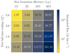 |
Fig. A.1. Heat map with integrated flux values calculated from the flux distributions presented in Fig. 11. |
All Tables
All Figures
|
Fig. 1. Schematic flowchart of the galaxy-in-a-box model. The computation starts with generating the spatial (Sect. 2.2.1) and mass (Sect. 2.2.2) distributions of GMCs in the simulated galaxy. The GMC mass distribution serves as the input to the module generating the protostellar spatial, mass, and age distributions within individual star-forming clusters. Here, each randomly chosen GMC mass is an initial mass of the cluster. Having calculated these distributions, the model uses them to assign molecular outflow emission to each protostar within the cluster, based on the envelope mass–outflow intensity relation calculated using the Water Emission Database (Sect. 2.3). After repeating these calculations for all GMCs, the emission and mass of star-forming clusters are returned to the galaxy-in-a-box model. Subsequently, the model merges the spatial distribution of the initial GMCs with water emission emerging from the corresponding star-forming clusters. Once the model returns the expected emission from the galaxy, this raw galactic emission grid is convolved with a Gaussian beam, producing the integrated intensity image of the galaxy. In this flowchart yellow corresponds to the galactic part of the model (Sect. 2.2), green to the cluster model (Sect. 2.1), red to the last stage of the model, and blue to the external data input. |
| In the text | |
|
Fig. 2. Two-part spatial configuration used in the galaxy-in-a-box model mapped onto the image of M 51 from NASA’s Hubble Space Telescope (credit: NASA, ESA, S. Beckwith (STScI) and the Hubble Heritage Team (STScI/AURA)). The M 51 image was scaled to fit within the spatial size settings used in the model. The white squares represent the location of stellar clusters along the spiral arms. |
| In the text | |
|
Fig. 3. Water line luminosity at 988 GHz vs. bolometric luminosity for objects from WED used in the simulations, with inclusion of a few additional sources that were excluded from the simulations due to lack of Menv data (San José-García 2015). The solid black line shows the best-fit proportionality, the orange filled region corresponds to the 95% confidence region of the correlation, and the shaded red region represents the region that contains 95% of the measurements. |
| In the text | |
|
Fig. 4. Example integrated intensity map of the template galaxy with the standard setup. |
| In the text | |
|
Fig. 5. Water emission at 998 GHz vs. envelope mass (Menv) for objects from WED used in the simulations. Colors as in Fig. 3. |
| In the text | |
|
Fig. 6. Results of multiple model runs with varying power-law slopes α of molecular cloud mass distributions. Top: distributions of cluster emission derived for simulations with different power-law slopes α of molecular cloud mass distributions. The vertical dashed lines correspond to the median flux of each distribution. In the bottom box plot the interquartile ranges are presented. The notches in the boxes indicate the 95% confidence intervals around the median. The whiskers spread to the beginning (0%) and the end (100%) of the distributions. These are the mean distributions from a series of ten simulations for each varying parameter. Bottom: radial profiles of emission from the galaxies of the corresponding α values. The radial profiles were calculated from the center of the galaxy all the way to its outskirts. The solid lines correspond to the mean profiles derived from ten simulations, while the shaded regions represent the spread of the mean values based on their standard deviations. |
| In the text | |
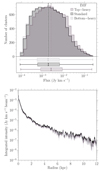 |
Fig. 7. As in Fig. 6, but for different IMF forms. |
| In the text | |
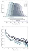 |
Fig. 8. As in Fig. 6, but for the varying εSF. |
| In the text | |
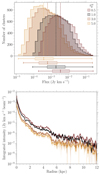 |
Fig. 9. As in Fig. 6, but for galaxies with different |
| In the text | |
|
Fig. 10. Total galactic emissions derived from all of the clusters averaged over ten simulations for each setup. The dashed black horizontal line corresponds to the standard setup described in Table 1. |
| In the text | |
|
Fig. 11. Distributions of cluster emission derived for simulations with varying free-fall time scaling factor |
| In the text | |
|
Fig. 12. Radial profiles of emission from the same set of simulations and color-coding as in Fig. 11. The solid lines correspond to the mean radial profile, while the shaded regions represent the variability of each profile, based on the standard deviation of each profile. |
| In the text | |
|
Fig. A.1. Heat map with integrated flux values calculated from the flux distributions presented in Fig. 11. |
| In the text | |
Current usage metrics show cumulative count of Article Views (full-text article views including HTML views, PDF and ePub downloads, according to the available data) and Abstracts Views on Vision4Press platform.
Data correspond to usage on the plateform after 2015. The current usage metrics is available 48-96 hours after online publication and is updated daily on week days.
Initial download of the metrics may take a while.