© Z. Brown et al. 2022

1 Introduction

Understanding the dynamics of inflation in the early universe is linked with the study of primordial density fluctuations, in particular with their deviations from a Gaussian distribution (see, e.g., Maldacena 2003; Bartolo et al. 2004; Acquaviva et al. 2003). High order correlations have been shown to be sensitive to non-Gaussian density fluctuations (see Meerburg et al. 2019 and references within). However, a brute force approach leads to prohibitively expensive O(Nⁿ) computations of correlations, where N is the number of tracer objects and n is the correlation order. This problem has been studied extensively (March 2013). Several approaches to mitigate it were suggested for the calculation of three-point correlations; for example, Yuan et al. (2018) used the small angle assumption, while Slepian & Eisenstein (2015) evaluated the Legendre expansion of the three-point correlation function (3pcf). The second approach was recently generalized for n-point correlation functions (npcfs) in Philcox et al. (2021) resulting in an O(N²) algorithm.

Here we present an alternative and computationally efficient way of evaluating these correlations. Similarly to March (2013), here this algorithm exploits spatial proximity, and similarly to Zhang & Yu (2011) and Slepian & Eisenstein (2016) it uses a fast Fourier transform (FFT) to speed up the calculation. These characteristics combined with implementation facilities help achieve a notable reduction in computational time and complexity.

The developed algorithm convolves kernels with matter maps, hence it is named ConKer¹. It is an extension of the CenterFinder algorithm (Brown et al. 2021), designed to find locations in space likely to be the centers of the baryon acoustic oscillations (BAOs). CenterFinder counts the number of galaxies removed from a particular location by a given distance by convolving spherical kernels with the matter distribution. ConKer uses the same functionality to evaluate npcfs. A similar approach was suggested in Slepian & Eisenstein (2016), and developed to evaluate the Legendre expansion of the 3pcf for continuous matter tracers in Portillo et al. (2018). In addition to implementing this approach for higher order correlations, ConKer introduces spatial partitioning defined with respect to the light of sight (LOS). This partitioning minimizes memory usage, allows for parallel computing, and enables an easy calculation of npcfs in the µ-slices, where the angle θ in the definition of µ = cos θ is measured with respect to the LOS.

ConKer is applicable to discrete matter tracers, such as galaxies, and to continuous tracers, such as Lyman-α and 21 cm line intensity, or matter maps derived from weak lenses. The method can be applied to evaluate autocorrelations, and cross-correlations between different matter tracers.

2 Algorithm description

2.1 Strategy

The two-point correlation can be visualized as an excess (or deficit) of sticks of a given length over a random combination of two points distributed over space. The three-point correlation corresponds to an excess of triangles, the four-point correlation to an excess of pyramids (the four points do not necessarily lie in one plane), and so on (see Fig. 1). We refer to these figures as n-pletes. We consider all possible n-pletes with one vertex at point 0, characterized by a vector r with the other vertices defined by vectors r_i, (i = 1, …n − 1). For each point we define a vector connecting it with point 0: s_i = r_i − r. We refer to a unit vector corresponding to any vector v as $\widehat{v}$.

We let ρ(r) be the density of the matter tracer (e.g., galaxy count per unit volume) at a location r, with $\overline{\rho }\left(r\right)$ being the density of expected observations from tracers randomly distributed over the surveyed volume. We define the deviation from the expected density as $$\Delta \left(r\right)=\rho \left(r\right)-\overline{\rho }\left(r\right).$$(1)

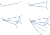Fig. 1 Cartoon illustrating the two-point correlation (0 – 1), three-point correlation (0 – 1 – 2), four-point correlation (0 – 1 – 2 – 3), and n-point correlation (0 – 1 – 2 – 3 – … - (n − 1)).

2.1.1 Isotropic npcf

The isotropic (averaged over the orientations of s_i) n-point correlation function is defined as $${\xi }_n^{iso}\left(s_1,\dots s_{\left(n-1\right)}\right)=\frac{1}{R_n^0}{\displaystyle \int \Delta \left(r\right)\Delta \left(r_1\right)\dots \Delta \left(r_{\left(n-1\right)}\right)d{\widehat{s}}_1\dots d{\widehat{s}}_{\left(n-1\right)}\text{d}r}$$(2)

where the integration over r implies all possible positions of point 0 in the surveyed volume. The normalization $R_n^0$ is evaluated by performing the same integration over the random distribution of tracers: $$R_n^0={\displaystyle \int \overline{\rho }\left(r\right)\overline{\rho }\left(r_1\right)\dots \overline{\rho }\left(r_{\left(n-1\right)}\right)d{\widehat{s}}_1\dots d{\widehat{s}}_{\left(n-1\right)}\text{d}r.}$$(3)

ConKer computes the integral of the matter density field over ${\widehat{s}}_i$ by placing a spherical kernel K_i of radius s_i on point 0 and taking its inner product with the ∆-field. For correlation order n, this implies a convolution of n − 1 kernels. This is illustrated in Fig. 2 for the three-point correlation. The sum of the product of the kernel with the matter density field is computed for a given location of point 0. Then the kernel is moved to a different location, thus scanning the entire surveyed volume and creating n − 1 maps of convolutions of kernels with the ∆-field. After this, the products of these maps and the original map of density fluctuations ∆(r) are summed over to produce the integral over r in Eq. (2). To evaluate $R_n^0$ the same procedure is performed on the random distribution of tracers.

2.1.2 Legendre expansion

We let θ_i indicate the angle between a vector s_i and r (see Fig. 2). We define the basis as a product of the Legendre polynomials, ${\text{Π}}_L\left(\cos {\theta }_i\right)=P_{l_1}\left(\cos {\theta }_1\right)P_{l_2}\left(\cos {\theta }_2\right)\mathrm{..}{P}_{l_{\left(n-1\right)}}\left(\cos {\theta }_{\left(n-1\right)}\right)$, where L = (l₁, l₂,…l_(n−1)) represents orders in the Legendre expansion. The angular dependence of the npcf can be characterized via a decomposition in this basis: $${\xi }_n\left(s_1,\dots s_{\left(n-1\right)}\right)={\displaystyle \sum _L{\xi }_n^L\left(s_1,\dots s_{\left(n-1\right)}\right){\text{Π}}_L\left(\cos {\theta }_i\right).}$$(4)

The coefficients ${\xi }_n^L$ in this expansion are functions of the distances s_i, but not the angles θ_i.

Following the example of Slepian & Eisenstein (2015) and its generalization (Philcox et al. 2021), we use the spherical harmonic addition theorem: $$P_l\left(\cos {\theta }_i\right)=\frac{4\pi }{2l+1}{\displaystyle \sum _{m=-l}^l{Y}_{lm}^{*}\left(\widehat{r}\right)Y_{lm}\left({\widehat{s}}_i\right)}.$$(5)

The evaluation of ${\xi }_n^L$ is then reduced to $${\xi }_n^L\left(s_1,\dots s\left(n-1\right)\right)=\frac{1}{R_n^0}{\displaystyle \int \text{d}r\Delta \left(r\right){\displaystyle \sum _{m_1}\mathrm{..}}{\displaystyle \sum _{m_{n-1}}\mathrm{..}}{C}_{LM}}{a}_{l_1{m}_1}^{*}\dots a_{l_{\left(n-1\right)}{m}_{\left(n-1\right)}},$$(6)

where coupling coefficients C_LM with M = (m₁, m₂, …m_(n−1)) are defined in terms of Wigner 3-j symbols (see Appendix A). The values of m_i are scanned from −l_i to +l_i. The calculation of the coefficients, $$a_{lm}\left(r,s_i\right)={\displaystyle \int \text{Δ}\left(r+s_i\right)Y_{lm}\left({\widehat{s}}_i\right)\text{d}{\widehat{s}}_i}$$(7)

implies an integration over all possible orientations of vector ${\widehat{s}}_i$. It is equivalent to convolving the matter density with a sphere of radius s_i centered on point 0 and populated with the values of Y_lm.

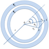Fig. 2 Cartoon illustrating a three-point correlation (0 – 1 – 2) with different scales s1 on the side (0 – 1) and s2 on the side (0 – 2). Integration over spherical shells K1 and K2 is equivalent to counting all possible triangles that have one vertex at point 0 and the other two anywhere on the spheres. For the calculation of ${\xi }_3^{\text{iso}}\left(s_1,s_2\right)$, the kernels are uniformly populated, while for the evaluation of the Legendre expansion coefficients ${\xi }_3^{l_1,l_2}\left(s_1,s_2\right)$ they are populated with the values of $Y_{l_i{m}_i}\left(i=1,2\right)$. The values of mi are scanned from −li to +li, resulting in 2(2l + 1) convolutions for each value of l, since both real and imaginary parts of Ylm must be used.

2.1.3 Edge correction

Irregular survey boundaries and nonuniformities in the redshift selection function can introduce anisotropies in an otherwise isotropic distribution. The formalism to correct for the edge effects developed in Slepian & Eisenstein (2015) and Philcox et al. (2021) is ideal for implementation using the kernel convolution functionality. The procedure involves the evaluation of Legendre moments of the random distribution $f_n^L$ according to Eqs. (6) and (7) with the $\overline{\rho }$-field used instead of ∆. In ConKer this is realized by convolving spherical kernels populated with the values of Y_1m with the random distribution of tracers.

A set of edge-corrected Legendre coefficients ${\widehat{\xi }}_n^L$ are calculated based on uncorrected ${\xi }_n^L$ evaluated using Eq. (6) and coefficients $f_n^L$ by solving a system of linear equations $${\widehat{\xi }}_n^L=M_{L{L}^{\prime }}^{-1}{\xi }_n^{L^{\prime }},$$(8)

where the matrix M_LL′ is defined as $$M_{L{L}^{\prime }}={\displaystyle \sum _K{\left(-1\right)}^{{\displaystyle \sum {l^{\prime }}_i}}{G}_{LK{L}^{\prime }}{f}_K.}$$(9)

For the definition of the Gaunt integral G_LKL′, see Appendix A.

2.2 Input

The inputs to the algorithm are catalogs of the observed number count of tracers D, with the total number being N_D, and R, which represents a number count of randomly distributed points within the same fiducial volume and corresponding number count N_R. Most surveys provide the angular coordinates: right ascension α and declination δ, and the redshift z of each tracer. The relationship between the redshift and the comoving radial distance is cosmology dependent: $$r\left(z\right)=\frac{c}{H_0}{\displaystyle {\int }_0^z\frac{d{z}^{\prime }}{\sqrt{{\text{Ω}}_M{\left(z^{\prime }+1\right)}^3+{\text{Ω}}_k{\left(z^{\prime }+1\right)}^2+{\text{Ω}}_{\Lambda }}}.}$$(10)

Here Ω_M, Ω_k, and Ω_Λ are the relative present-day matter, curvature, and cosmological constant densities, respectively; H₀ is the present-day Hubble constant; and c is the speed of light. These user-defined parameters represent the fiducial cosmology. In this study we used the following values for the cosmological parameters: c = 300 000 km s⁻¹, H₀ = 100h km s⁻¹ Mpc⁻¹, Ω_M = 0.29, Ω_Λ = 0.71, and Ω_k = 0. The integral in Eq. (10) is evaluated numerically in ConKer. Cartesian coordinates of a tracer labeled (X,Y,Z) are evaluated based on r, α, and δ.

The algorithm computes correlation functions over a given range of scales or separation distances s_i. The range of distances from s_min to s_max is divided into N_b bins, which sets the bin width ∆s.

2.3 Partitioning and mapping

The initial step of the algorithm divides data and random catalogs into partitions based on the angular variables (α, δ). Each partition spans the entire range of redshifts from z_min to z_max corresponding to the co-moving radii r_min and r_max, evaluated according to Eq. (10). The angular size θ_p is determined by the angle subtended by s_max at r_min: $${\theta }_p=\frac{s_{\max }}{r_{\min }}.$$(11)

Each (jk)th partition is populated by galaxies with angular coordinates within the following limits: $${\alpha }_{j-1}\to {\alpha }_j={\alpha }_{j-1}+\frac{2{\theta }_p}{\min \left(\cos {\delta }_k\right)},$$(12) $${\delta }_{k-1}\to {\delta }_k={\delta }_{k-1}+2{\theta }_p.$$(13)

Here min(cos δ_k) is the minimum value of cos δ_k in this partition. This factor is introduced for each region to have an approximately square span of 2s_max in the azimuthal and polar directions at the smallest comoving radius. The lowest boundaries are determined by the survey coverage.

The definition of the Cartesian $\left(\widehat{x},\widehat{y},\widehat{z}\right)$ system is unique to each partition with the $\widehat{x}$-axis pointing to its center cell. The transformation from global sky to local Cartesian coordinates is given in Appendix B.

The LOS in each partition is defined as pointing along the $\widehat{x}$-axis. Having the same definition of the LOS for all the objects in the partition introduces some inaccuracy in angles, especially for objects near the boundary. However, the maximum deviation in the LOS definition is on the order of ${\theta }_p^2/2$. Hence, this inaccuracy can be minimized by the proper choice of the partition size θp.

In each partition we define a grid with spacing g_S, such that the volume of each cubic grid cell is $g_S^3$. The default value of g_S is set to be equal to the bin width ∆s. However, the user can select a finer resolution in the density field and kernels. In this case, g_S is set to a desired fraction of the radial bin size ∆s. During the final steps of the algorithm, correlation functions are resampled to the appropriate s-bins.

On the grid we define three-dimensional histograms, D(X, Y, Z) and R(X, Y, Z), which represent tracer counts in the cell (X, Y, Z) from data and random catalogs, respectively. These histograms may be populated by the raw count or the weighted count of tracers from the input catalogs.

In every partition two additional grids are constructed, D_MP(X, Y, Z) and R_MP(X, Y, Z), which contain an extended map of objects within an additional θp in the declination direction and an additional θ_p/min(cos δ_k) in the right ascension direction of the LOS. During the convolution step the center of the kernel is placed on each cell of D(X, Y, Z) and R(X, Y, Z), while the convolution is performed with the extended maps D_MP(X, Y, Z) and R_MP(X, Y, Z). This procedure ensures that the entire survey region is covered, but that double-counting is avoided².

A three-dimensional local density variation histogram N(X, Y, Z), which is a discretized representation of the ∆ field, is defined on the grid to represent the difference in counts between D and R, normalized to N_D: $$N\left(X,Y,Z\right)=D\left(X,Y,Z\right)-R\left(X,Y,Z\right).$$(14)

A similar field N_MP(X, Y, Z) is defined using the extended grids.

The default mass assignment scheme used in ConKer is a three-dimensional histogram, or nearest grid point (NGP) method. However, Jing (2005) and Cui et al. (2008) showed that the galaxy power spectrum measured using FFT algorithms is sensitive to the choice of mass assignment scheme. The ConKer algorithm includes the option to use the cloud in cell (CIC) method when defining the density fields. Of the two methods, CIC is more computationally expensive since it maps each tracer to multiple grid cells. The stage of the algorithm that places matter tracers in grid cells is referred to as mapping.

2.4 Kernels

We construct spherical kernels $K_i^{lm}\left(X,Y,Z\right)$ on a cube, just large enough to encompass a sphere of radius s_i + ∆s/2. The grid defined on this cube has the same spacing g_S as that used to construct the density fields. The cube is extended to have an odd number of cells in each coordinate direction. This ensures that it has a well-defined center cell, the center of which defines the center of the kernel.

We construct a spherical shell of the inner radius s_i − ∆s/2 and the outer radius s_i + ∆s/2 centered on the center of the kernel. A numeric value is assigned to each kernel cell. If none of a cell’s volume falls within the shell, it is assigned 0. If, however, any part of the cell is within the shell, it is assigned the value that corresponds to the fraction of its volume within the shell. This is realized by considering a user defined number of random positions within the each cell. We refer to this kernel as “flat”.

If the user has elected to employ a grid resolution g_S finer than the desired radial binning, an integer number of extra kernels are constructed between the limits of each s-bin, where the integer gives the rate of resampling. For example, to resample correlation functions at twice the desired radial binning, 2g_S = ∆s and a factor of two additional kernels are constructed for each s-bin.

2.4.1 Kernels for Legendre expansion

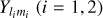
We let l_max be the largest Legendre multipole probed in the evaluation of the npcf. For each l from 0 to l_max, and each m from −l to +l, we compute the spherical harmonic Y_lm(θ_K, ϕ_K), where θ_K is the polar angle with respect to the kernel’s $\widehat{x}$-axis, and ϕ_κ is the azimuthal angle. In each nonzero cell the kernel $K_i^{lm}\left(X,Y,Z\right)$ is assigned values equal to the product of the flat kernel with the average of Y_lm, evaluated over the region of the kernel cell corresponding to the radial limits. The averaging is done during the same procedure of random sampling as used in the construction of the flat kernel. For cases when m ≠ 0, real and imaginary kernels are constructed using R[Y_lm] and J[Y_lm]. Kernels of various configurations are shown in slices along the LOS direction in Fig. 3.

2.4.2 Kernels for µ-slices

There is a class of problems (e.g., redshift distortion studies) where it is important to evaluate npcfs in several µ-slices (Sánchez et al. 2017). The parameter µ = cos θ is defined with respect to the LOS. The definition of LOS is the same through the entire partition, as discussed in Sect. 2.3, which introduces some inaccuracy for objects near the region’s boundary. For example, a maximum scanned distance of s_max = 150 Mpc h⁻¹ and a minimum redshift of z_min = 0.4 result in an upper boundary on the inaccuracy in the LOS definition of 0.8%. For interior objects and higher redshifts it is even smaller. The application of µ-slices is naturally implemented via a definition of kernel K_µ,i that is not populated over the entire sphere, but rather in a section corresponding to the desired range of µ, as shown in Fig. 4. They are normalized such that a complete µ-wedge kernel from µ = 0 to µ = 1 is identical to the l = 0 kernel used in the Legendre expansion.

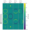Fig. 3 Two-dimensional slices of spherical kernels, radius 108 h−1 Mpc, gS = 8 h−1 Mpc. The slices are transverse to the LOS direction moving outward (top to bottom). The value of kernel cells is shown for four configurations: l = 0, m = 0 (real); l = 2, m = 0 (real); l = 2, m = 1 (real); l = 2, m = 1 (imaginary).

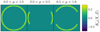Fig. 4 Two-dimensional slices of spherical kernels, radius 108 h−1 Mpc, gS = 8 h−1 Mpc. The slices are along the LOS direction. The value of kernel cells is shown for three configurations corresponding to a complete wedge (0.0 < µ < 1.0), ξ⊥ (0.0 < µ < 0.5), and ξ∥ (0.5 < µ < 1.0).

2.5 Convolution

We construct a three-dimensional histogram $W_i^{lm}\left(X,Y,Z\right)$ with entries equal to the inner product of kernel $K_i^{lm}$ centered on a cell with coordinates (X, Y, Z) and matter density variation field N_mp(X, Y, Z): $$W_i^{lm}\left(X,Y,Z\right)\equiv N_{MP}\left(X,Y,Z\right)***K_i^{lm}\left(X,Y,Z\right).$$(15)

Here * * * denotes a three-dimensional discrete convolution performed using FFT and $W_i^{lm}$ is a discretized representation of coefficients a_lm calculated according to Eq. (7). The procedure is performed in each partition, for each bin in s and for all possible values of l and m according to a given l_max, resulting in 2(l_max + 1)²N_b convolutions. Once these maps of $W_i^{lm}\left(X,Y,Z\right)$ are created, they can be used to calculate the correlation functions of arbitrary order n.

For normalization purposes we perform the same procedure on the field of random counts. The result of the convolution of random density field R_MP with kernel $K_i^{lm}$ is referred to as $B_i^{lm}\left(X,Y,Z\right)$: $$B_i^{lm}\left(X,Y,Z\right)\equiv R_{MP}\left(X,Y,Z\right)***K_i^{lm}\left(X,Y,Z\right).$$(16)

For the calculation of the normalization factor $R_n^0$, only convolution with the isotropic kernel (l = 0, m = 0) is required. However, for the edge correction the convolution of K^lm with the random catalog for all values of l and m is needed. Often a large ensemble of simulated catalogs, or mocks, each having the same survey boundaries is considered. In this case the convolution of all kernels with the random catalog needs only be performed once. This allows for a significant reduction in computation time and disk-space allocation. In the case corresponding to the µ-slice kernels, the convolution step is nearly identical, replacing only $K_i^{lm}$ with the appropriate kernel, K_µ,i, and repeating for each desired bin in µ. This stage of the algorithm is referred to as convolution.

2.6 Memory management

The mapping and especially convolution steps produce multiple large three-dimensional grids, $W_i^{lm}$ and $B_i^{lm}$; however, it is not feasible to store them in their entirety in the RAM of almost any computer. Thus, during the convolution step of the algorithm, ConKer writes each unique grid to a temporary file. The user can chose to save the entire grid as a three-dimensional array or to sparcify it. Sparcification is marginally more time consuming, but saves a considerable amount of disk space.

During this step of the algorithm, referred to as file operations, the grids are temporarily stored for the following summation step.

2.7 Evaluation of n-point correlation functions

For each (jk)th partition we concatenate every grid $W_i^{lm}$ and $B_i^{lm}$ such that they now represent a convolution of the kernel with the entire density field. A map of $W_i^{lm}$ represents discretized coefficients $a_i^{lm}$ in Eq. (6). According to this equation to evaluate coefficients ${\xi }_n^L$ these maps must be convolved with the matter distribution ∆(r), a discretized representation of which is N(X, Y, Z), and summed over the entire grid. Hence, $${\xi }_n^L\left(s_1,\dots s_{\left(n-1\right)}\right)=\frac{{\sum }_{\text{grid}}{W}_0{\sum }_{m_1}\mathrm{..}{\sum }_{m_{\left(n-1\right)}}{C}_{LM}{W}_1^{*l_1{m}_1}\mathrm{..}{W}_{n-1}^{l_{n-1}{m}_{n-1}}}{{\sum }_{\text{grid}}{B}_0{B}_1^0\mathrm{..}{B}_{n-1}^0},$$(17)

where W₀ = N(X, Y, Z) and B₀ = R(X, Y, Z). This step in the algorithm is referred to as summation.

2.7.1 Cases

The specific case of lth multipole of the 2pcf is calculated as $${\xi }_2^l\left(s\right)=\frac{1}{\sqrt{2l+1}}\frac{{\sum }_{\text{grid}}{W}_0{W}_1^{l0}}{{\sum }_{\text{grid}}{B}_0{B}_1^0}.$$(18)

The lth multipole of the 3pcf is then calculated as $${\xi }_3^l\left(s_1,s_2\right)=\frac{4\pi }{\sqrt{2l+1}}\frac{{\sum }_{\text{grid}}{W}_0{\sum }_m{W}_1^{*lm}{W}_2^{lm}}{{\sum }_{\text{grid}}{B}_0{B}_1^0{B}_2^0}.$$(19)

This procedure is repeated on the random field in order to construct the terms necessary for edge-correction (see Philcox et al. 2021): $$f_3^l\left(s_1,s_2\right)=\frac{4\pi }{\sqrt{2l+1}}\frac{{\sum }_{\text{grid}}{B}_0{\sum }_m{B}_1^{*lm}{B}_2^{lm}}{{\sum }_{\text{grid}}{B}_0{B}_1^0{B}_2^0}.$$(20)

At the summation stage, computing the npcf requires that the already computed grids defined by s, l, and m be combined and summed over. The execution time of this step is about two orders of magnitude lower than the convolution step in the case of the 3pcf, and trivial in the case of the 2pcf. Only at very large correlation orders does the execution time of the summation process begin to approach that of convolution.

Of particular interest are correlations between objects with a defined scale, such as those arising from spherical sound waves in the primordial plasma, also known as BAOs. In this case one tracer taken as a starting point is displaced from the other (n − 1) points by the same distance s₁ (e.g., the three-point correlation corresponds to isosceles triangles randomly distributed in space). This equidistant case corresponds to the diagonal of the n-point correlation function (hence referred to as the diagonal npcf) for l = 0, which is calculated as $${\xi }_n^{0,\text{diag}}\left(s\right)=\frac{{\sum }_{\text{grid}}{W}_0{\left(W_1^0\right)}^{n-1}}{{\sum }_{\text{grid}}{B}_0{\left(B_1^0\right)}^{n-1}}.$$(21)

One of the advantages of the ConKer algorithm is that regardless of the desired correlation order, n, no new convolution operations need take place. Thus, the time-consuming step is only performed once per catalog, which facilitates subsequent calculations of correlation functions to arbitrary order, n.

2.8 Procedure

A schematic flowchart of the ConKer algorithm is shown in Fig. 5. Beginning with a definition of the cosmological parameters and binning, the partitioning is performed on the random catalog. If that catalog has already been used, the previous partitioning scheme is employed. During the convolution step, the user can choose whether or not to perform the convolution with the catalog of random tracers for edge correction. It is more time consuming, but only needs to be performed once per random catalog. During the summation step the user is able to compute an arbitrary number of correlation functions of a desired order n and l_max. Since files corresponding to the convolved grids are often large, the user can choose to delete them upon completion of the summation step.

If the user wishes to employ the µ-wedge kernels, the procedure is nearly identical; however, each step of the calculation must be repeated for each slice. This increases the relevant computational parameters such as run time and file sizes, but does not affect memory considerations as the calculations in each slice are performed independently.

3 Performance study

We evaluated the performance of ConKer using SDSS DR12 CMASS galaxies (Ross et al. 2017), their associated random catalogs, and an ensemble of MultiDark-Patchy mocks (Kitaura et al. 2016; Rodríguez-Torres et al. 2016). We applied ConKer to the SGC and NGC catalogs for data, randoms, and 20 mocks. For this study, which highlights the algorithm’s ability to probe correlations near the clustering and the BAO scales, we computed correlation functions for a distance range of 8–176 h⁻¹ Mpc in 21 bins of width of 8 h⁻¹ Mpc. In all cases, the standard systematic (Ross et al. 2017) as well as FKP weights (Feldman et al. 1994) were used to create the density field map. The default NGP mass assignment scheme was used and the grid spacing of g_S = 8 h⁻¹ Mpc unless specified otherwise.

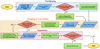Fig. 5 ConKer flowchart. Parameters or settings chosen by the user are in blue, internal processes are in green, and decisions made by the user are in red.

3.1 Timing study

We demonstrate the efficient nature of our algorithm with the following timing study, performed using a personal computer with a 10 CPU core Apple M1 Pro chip and 32 GB of memory. All execution times are in units of CPU seconds.

The primary advantage of ConKer is in the behavior of the execution time as a function of the total number of objects N = N_D + N_R shown in top plot of Fig. 6 for the four stages of the algorithm: mapping, convolution, file operations, and summation. The surveyed volume, V is kept fixed. As expected, the execution time of convolution, file operations, and summation are nearly independent of N, and all three scale below O(N^1/2). Mapping is an O(N) calculation, and only starts to dominate for catalogs significantly larger than 100M objects.

The main parameter that determines the computation time of ConKer is the grid spacing g_S, which is set by default to be equal to the bin width ∆s. The maximum distance probed s_max determines the number of steps in s: N_b = (s_max − s_min)/∆s. The total number of grid cells N_c depends on the surveyed volume: $N_{\text{c}}=V\text{/}{g}_S^3$. Mapping is independent of g_S. For g_S below approximately 5 h⁻¹ Mpc, the dominant process is convolution of cubic volumes, on which the kernels are defined, containing N_k cells: N_k = (s/g_s)³ < (s_max/g_S)³. It is repeated N_c times with each grid cell being the center of the kernel. Since the convolution is performed using FFT with a typical complexity of N log N, the complexity of each step in s is O(N_c log N_k). Thus, the time complexity of the convolution is $$t_{\text{conv}}\propto N_b{N}_{\text{c}}\log N_k<\frac{s_{\max }}{g_S}\frac{V}{g_S^3}\log \frac{V_k}{g_S^3}\propto g_S^{-4}\log g_S\propto N_{\text{c}}^{4/3}\log N_{\text{c}}.$$(22)

The observed scaling of the convolution step as $g_S^{-4.3}$ is in good agreement with this analytic prediction as depicted by the solid brown line in Fig. 6 (bottom).

The file operations step scales more favorably with g_S; however, it dominates the execution time for g_S above approximately 5 h⁻¹ Mpc.

3.2 Comparison to existing methods

We present comparisons of the 2pcf and 3pcf evaluated using ConKer to well-established methods. In Cuesta et al. (2016) the monopole and quadrupole terms of the Landy and Szalay estimator of the 2pcf (Landy & Szalay 1993; Hamilton 1993) are computed for the combined SGC and NGC catalogs of the SDSS DR12 CMASS survey galaxies. We performed the calculation using ConKer with the same binning, and compared it to the Cuesta et al. (2016) results in Fig. 7. For the monopole and the quadrupole terms, we note good agreement between the two methods. At low scales (s < 30 h⁻¹ Mpc), we find the largest deviation between the two. The differences expectedly arise due to the discretization of the density field and kernel in ConKer. The kernel represents a spherical shell of width g_S mapped onto a three-dimensional Cartesian grid. Thus, once the kernel size becomes comparable with the grid spacing a resolution in the distance determination is degraded. This occurs, when the kernel size is less than approximately 5g_S. This does not mean, however, that we are unable to probe correlations at small scales. Instead, this simply requires a finer grid, and resampling. By reducing the grid spacing (blue and red points in Fig. 7) we recovered the agreement down to lower scales. Based on this, we recommend setting the s_min parameter larger than 5∆s if using the default sampling. Any differences in the size of the errors results from the fact that we use two separate mock ensembles to estimate the covariance.

In addition to the Legendre expansion, we also compute the 2pcf of the NGC sample in two µ-slices, corresponding to the transverse (ξ_⊥) and parallel (ξ_∥) cases. To compare, we repeated the calculation using nbodykit, an open source cosmology toolkit (Hand 2018). The results are shown in Fig. 8. We find the same behavior at small scales as in the case of the Legendre expansion, where the agreement is recovered by reducing the grid spacing.

In Figs. 7 and 8 comparing the l = 0,2 and ξ_±‖ cases to existing clustering algorithms, the uncertainties on the survey data measurements were derived from the mock ensemble. The size of the error bar corresponding to point-i is ${\sigma }_i=\sqrt{C_{ii}}$, where C is the mock covariance matrix.

The 3pcf algorithm implemented in nbodykit is based on the work of Slepian & Eisenstein (2015). Using the two methods, we computed the edge-corrected 3pcf up to l = 3 of the same subsample of NGC galaxies used in the timing study (see caption of Fig. 6 for details). The 3pcf, using both estimators, is shown in Fig. 9, as well as the distributions of the differences between them. For this comparison, we computed 3pcf in 11 bins of width of 10 h⁻¹ Mpc for s from 45 to 155 h⁻¹ Mpc. Over this range of scales, we find a good agreement between the two methods. By convention, the diagonal terms of the 3pcf are excluded in this comparison (see Slepian & Eisenstein 2015).

More importantly, the distribution over the residuals is centered at approximately zero, meaning our estimator is not biased compared to the nbodykit implementation. The largest deviations between the algorithms again arise at smaller scales where the kernel resolution is degraded. The 3pcf calculation using ConKer was faster by a factor of ~3, and scales more favorably with N, since nbodykit is an O(N²) algorithm.

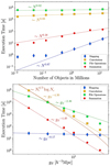Fig. 6 Execution time of the four processes in the ConKer algorithm, as applied to subsamples of the SDSS DR12 CMASS NGC galaxies (150° < αg < 210°, 0° < δg < 60°). Each point represents a calculation of the 2pcf (l = 0,2,4), 3pcf (l = 0–5), and diagonal npcf up to n = 5. Top: dependence on the number of combined data and random objects, using a grid resolution gS = 8 h−1 Mpc. Bottom: dependence on the grid resolution gS for 12.5M objects. The points represent the measured CPU time. The dashed lines are the results of the fit to a power law, with the scaling given in the figure. The solid line (bottom) is the time of the convolution step fit to $N_{\text{c}}^{4/3}\log N_{\text{c}}$.

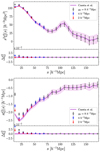Fig. 7 A comparison of the 2pcf as measured by the ConKer algorithm versus existing clustering algorithms. Top: 2pcf monopole ${\xi }_2^0\left(s\right)$ computed using ConKer with three different values of grid spacing gS = 8 (grey), 4 (blue), 2 (red) h−1 Mpc, and results from Cuesta et al. (2016) (purple line). Finer grids were resampled to ∆s = 8 h−1 Mpc bins. The error bars on the ConKer points were extracted from the covariance matrix of the Patchy mock ensemble. The errors in Cuesta et al. (2016; shaded region) are from an ensemble of quick particle mesh mocks (White et al. 2014). The 2pcf is multiplied by s2 to emphasize features at large scales. The lower subpanel shows the residual between the two methods. Bottom: same as the top panel, but for the 2pcf quadrupole ${\xi }_2^2\left(s\right)$. Here, the 2pcf is multiplied by s instead of s2 by convention.

3.3 ConKernpcf

We used ConKer to compute the diagonal elements of the npcf as defined in Eq. (21) for n = 2,3,4,5 and l = 0, and off-diagonal elements of the 3pcf for an ensemble of MultiDark-Patchy mocks. For this calculation, the NGC/SGC catalogs were divided into 27/14 partitions, as shown in Fig. 10.

The diagonal elements of the npcfs are shown in Fig. 11 for n = 2,3,4, and 5. We observe the expected features of the npcfs. These include an increase in magnitude at small scales present for n = 2 and n = 3, corresponding to galaxy clustering, and a well-defined “bump” at the BAO scale for all. The npcfs based on the random catalog fluctuate about ξ_n = 0 at several orders of magnitude below the signal observed in mocks.

In each case, the covariance matrix of the diagonal npcf is estimated on the set of 20 Patchy mocks using the following procedure. For the ith bin of the npcf, we let the average value across the mock ensemble be defined as <ξ>_i. If the number of mocks in the ensemble is N_q, then the covariance matrix elements are $$C_{ij}=\frac{1}{N_q-1}{\displaystyle \sum _q\left({\xi }_n^{0,\text{diag}}\left(s_i\right)-<\xi {>}_i\right)\left({\xi }_n^{0,\text{diag}}\left(s_j\right)-<\xi {>}_j\right).}$$(23)

We show an example of the reduced covariance matrix for the n = 2, l = 0 diagonal case in Fig. 12.

Off-diagonal elements of the edge-corrected 3pcf are shown in Fig. 13 for the NGC sample. Emphasizing for large-scale features, we observe strong indicators of BAO in both the l = 0 and l = 1 cases.

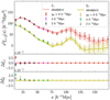Fig. 8 Points showing the transverse ξ⊥(s) and parallel ξ‖(s) components of the 2pcf computed using ConKer with three values of grid spacing gS = 8 (red–yellow), 4 (purple–green), 2 (black–grey) h−1 Mpc. Solid lines in the corresponding colors show the results from the nbodykit 2pcf algorithm. This figure corresponds only to NGC galaxies. The error bars and shaded regions are determined from the ensemble of Patchy mocks. The lower subpanels show the residual between the two methods.

4 Discussion

4.1 Algorithmic framework

The query for a pattern in matter distributions may prompt the employment of machine learning techniques. ConKer, being a spatial statistics algorithm, offers an alternative to such an approach that is fast and transparent. It exploits the fact that the full set of equidistant points from any given point makes a sphere, with its surface density being a direct measure of how spherically structured this subspace of points is. Aggregating and combining this measure over the whole space of N objects allows us to calculate the space’s n-point correlation function.

The algorithm exploits an intrinsic spatial proximity characteristic in the objective of querying structures of negligible dimensions in a much bigger space. This spatial proximity factor leads to space partitioning algorithms targeting a nearest neighbor query approach (see, e.g., the tree-based npcf algorithms in March 2013). However, ConKer uses this factor as a heuristic in limiting its query space immediately to only the defined separation for each point in the space. We note how this is in contrast with the former technique family. In a nearest neighbor approach to the npcf problem, the query space is grown at each point in the greater embedding space, aggregating the n-point statistic until the greater space is fully queried, whereas ConKer aggregates the statistic over all embedding space, and then grows the query space before repeating.

This design choice realized in ConKer’s core subroutine, a convolution of the query space with the embedding space performed by an FFT algorithm, distills the complexity from the brute force. This approach, combined with the heuristic above, lets the dominant components of ConKer achieve independence of the number of objects, as shown in Fig. 6. There is certainly a trade-off between the sparsity of the whole space and the bias toward linear complexity in number of objects, as expected from an FFT-based algorithm, but even for very dense catalogs, we expect the scaling in the number of objects to be capped by O(N), where N is the total number of objects. Ultimately, ConKer is a hybrid algorithm that draws from both computational geometry and signal processing to achieve linear complexity in the number of objects.

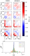Fig. 9 A comparison of the 3pcf estimated using ConKer compared to existing methods. Top: edge-corrected 3pcf, ${\xi }_3^l\left(s_1,s_2\right)$, computed using ConKer (left column) and nbodykit (right column) up to l = 3. The color scale is applicable to all panels. Bottom: residual between the two methods, shown as a distribution over all (s1, s2) pairs for l = 0 (blue), l = 1 (yellow), l = 2 (green), and l = 3 (red).

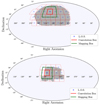Fig. 10 Angular footprint of the NGC (top) and SGC (bottom) galaxies (grey dots), divided into partitions (dashed red lines), each with a unique LOS (blue marker). The solid red line highlights one such partition. During the convolution step, the center of the kernel is positioned within these boundaries, while the convolution is performed over the region bound by the solid green line.

4.2 ConKer versus other methods

The idea of convolving spherically symmetric kernels with the density fields to evaluate the number of objects removed from a certain point by a given distance was originally proposed in Zhang & Yu (2011). In this work the Legendre expansion of npcf was not considered. In Slepian & Eisenstein (2015) and Philcox et al. (2021) a KdTree algorithm was used and the spherical function decomposition was evaluated for each galaxy pair, resulting in O(N²) calculation. This method works well for smaller scales or sparse surveys. In the same papers using FFT-based convolution for the Legendre expansion was also suggested. This approach has an advantage for denser surveys or continuous tracers since the computational time depends on the volume but not on density. The idea was later realized in (Portillo et al. 2018) for the evaluation of the 3pcf of the continuous tracer.

ConKer extends the approach to all n > 1. ConKer computes the integral in Eq. (7) by convolving a spherical kernel K_i of radius s_i populated with the values of Y_lm with the matter density field. The definition of a kernel on the grid necessarily leads to some loss of precision in the distance definition. This is partially mitigated in ConKer by weighting the grid cells with the fraction of the cell’s volume contained within a given spherical shell and averaging Y_lm’s over this volume. Convolving the entire surveyed volume (as in Portillo et al. 2018) leads to large arrays that need to be stored resulting in significant memory requirements. In light of anticipated large volume surveys such as DESI (DESI Collaboration 2016), this limitation becomes particularly stringent. ConKer convolves a cubic volume just large enough to encompass a sphere of the specified radius, thus limiting the memory requirements for kernel storage. Additionally, ConKer introduces a partitioning scheme, as discussed in Sect. 2.3. As a result, the array size is limited by the partition’s volume. This scheme has an additional benefit; it allows for the evaluation of npcfs in µ-slices as, discussed in Sect. 2.4.2, which is particularly relevant for parallel versus transverse to the LOS analysis. Finally, partitioning naturally allows for parallelized computing processes.

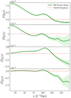Fig. 11 Diagonal npcf, ξn(s), from n = 2 to n = 5 (from top to bottom), for the combined SGC+NGC sample of the ensemble of MD Patchy mocks (green) and the associated randoms (red dashed line). The shaded green region around the mock average gives the errors computed from the diagonal elements of the mock co-variance matrix, C. The npcf is multiplied by a proxy for the total kernel volume, where $\tilde{s}=s\text{/}\left(100h^{-1}\text{\hspace{0.17em}Mpc}\right)$. This convention highlights features at large scales.

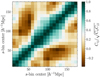Fig. 12 Reduced covariance matrix $C_{ij}\text{/}\sqrt{C_{ii}{C}_{jj}}$ for the n = 2 diagonal isotropic correlation function. It is computed from the ensemble of Patchy mocks.

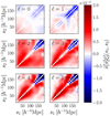Fig. 13 Three-point correlation function ${\xi }_3^l\left(s_1,s_2\right)$ of the NGC mock ensemble, computed up to l = 5. Multiplication by ${\tilde{s}}_1^2{\tilde{s}}_2^2$, emphasizes the same large-scale features as in Fig. 11. The diagonal elements are excluded from these plots.

4.3 Applications beyond correlation functions

Though traditionally the order of correlation n is viewed as an important parameter, for the diagonal npcf, all the information is entirely encoded by the weights W₀ and W₁. It was pointed out in Carron & Neyrinck (2012) that the npcf is inadequate in capturing the tails of non-Gaussianities. The distributions over W₀ and W₁ (as opposed to their sum over the sample, as is used in the npcf) could recover that sensitivity, which is a subject for future studies. The distribution of the product of two weights, W₀W₁ normalized by the average B₀B₁ is presented in Fig. 14 for a kernel size of 108 h⁻¹ Mpc for data, mock, and random catalogs.

Moreover, W₀ and W₁ as well as their product are maps. While in the npcf the location information is entirely lost, in the maps produced by ConKer it is preserved and can be used for cross-correlation studies between different tracers, such as weak lensing, Lyα, and CMB.

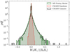Fig. 14 Distribution, W0W1/⟨B0B1⟩ at s1 = 108 h−1 Mpc, for the CMASS galaxy sample of the SDSS DR12 survey (black), one of the MD Patchy mocks (green), and the associated randoms (red). This plot includes NGC galaxies only.

5 Conclusion

We presented ConKer, an algorithm that convolves spherical kernels with matter maps allowing for fast evaluation of the n-point correlation functions, its expansion in Legendre polynomials, and its µ-slices. The algorithm can be broken into three stages: mapping, convolution, and summation. The execution time of convolution and summation are independent of the catalog size N, while mapping is a O(N) calculation, which starts dominating for catalogs larger than 100M objects. The dominant part of the convolution is with complexity $O\left(N_{\text{c}}^{4/3}\log N_{\text{c}}\right)$, where N_c is the number of grid cells.

A comparison to the standard techniques shows good agreement. We study the performance using SDSS DR12 CMASS galaxies, their associated random catalogs, and an ensemble of MultiDark-Patchy mocks. The results up to n = 5 are presented. Further metrics that may offer additional sensitivity to primordial non-Gaussianities are also suggested such as the distribution over weights W_i and their products.

Acknowledgements

The authors would like to thank Z. Slepian for his interest and insightful comments, F. Weisenhorn for assistance with the nbodykit 3pcf calculations, A. Ross for providing numeric values of SDSS DR12 CMASS 2pcf, and S. BenZvi, K. Douglass and S. Gontcho A Gontcho for useful discussions. The authors acknowledge support from the US Department of Energy under the grant DE-SC0008475.0. Funding for SDSS-III has been provided by the Alfred P. Sloan Foundation, the Participating Institutions, the National Science Foundation, and the US Department of Energy Office of Science. The SDSS-III web site is http://www.sdss3.org/. SDSS-III is managed by the Astrophysical Research Consortium for the Participating Institutions of the SDSS-III Collaboration including the University of Arizona, the Brazilian Participation Group, Brookhaven National Laboratory, Carnegie Mellon University, University of Florida, the French Participation Group, the German Participation Group, Harvard University, the Instituto de Astrofísica de Canarias, the Michigan State/Notre Dame/JINA Participation Group, Johns Hopkins University, Lawrence Berkeley National Laboratory, Max Planck Institute for Astrophysics, Max Planck Institute for Extraterrestrial Physics, New Mexico State University, New York University, Ohio State University, Pennsylvania State University, University of Portsmouth, Princeton University, the Spanish Participation Group, University of Tokyo, University of Utah, Vanderbilt University, University of Virginia, University of Washington, and Yale University. The massive production of all MultiDark-Patchy mocks for the BOSS Final Data Release has been performed at the BSC Marenostrum supercomputer, the Hydra cluster at the Instituto de Física Teorica UAM/CSIC, and NERSC at the Lawrence Berkeley National Laboratory. We acknowledge support from the Spanish MICINNs Consolider-Ingenio 2010 Programme under grant MultiDark CSD2009-00064, MINECO Centro de Excelencia Severo Ochoa Programme under grant SEV-2012-0249, and grant AYA2014-60641-C2-1-P. The MultiDark-Patchy mocks was an effort led from the IFT UAM-CSIC by F. Prada’s group (C.-H. Chuang, S. Rodriguez-Torres and C. Scoccola) in collaboration with C. Zhao (Tsinghua U.), F.-S. Kitaura (AIP), A. Klypin (NMSU), G. Yepes (UAM), and the BOSS galaxy clustering working group.

Appendix A Useful formulae

For L = (l₁, l₂, … l_(n−1)) and M = (m₁, m₂, …, m_(n−1)) with each −li ≤ m_i ≤ l_i we can define the coupling coefficient C_LM in terms of Wigner 3-j symbols (3×2 matrices) as $$\begin{array}{lll}\hfill C_{LM}& \hfill =& \hfill {\left(-1\right)}^{{\sum }^{l_i}}\sqrt{2l_{12}+\mathrm{1..}}\sqrt{2l_{\mathrm{12..}\left(n-3\right)}+1}{\displaystyle \sum _{m_{\mathrm{12..}}}{\left(-1\right)}^{\kappa }}\\ \hfill & \hfill & \hfill \left(\begin{array}{lll}\hfill l_1& \hfill l_2& \hfill l_{12}\\ \hfill m_1& \hfill m_2& \hfill -m_{12}\end{array}\right)\left(\begin{array}{lll}\hfill l_{12}& \hfill l_3& \hfill l_{123}\\ \hfill m_{12}& \hfill m_3& \hfill -m_{123}\end{array}\right)\\ \hfill & \hfill & \hfill \mathrm{..}\left(\begin{array}{lll}\hfill l_{\mathrm{12..}\left(n-3\right)}& \hfill l_{\left(n-2\right)}& \hfill l_{\left(n-1\right)}\\ \hfill m_{\mathrm{12..}\left(n-3\right)}& \hfill m_{\left(n-2\right)}& \hfill -m_{\left(n-1\right)}\end{array}\right),\end{array}$$(A.1)

where κ = l₁₂ − m₁₂ + l₁₂₃ − m₁₂₃ + ..l_(n−1) − m_(n−1).

The Gaunt integral G_L1L2L3 used in the edge correction procedure is defined as $$G_{L_1{L}_2{L}_3}={\displaystyle \int d\widehat{r}{\text{Π}}_{L_1}\left(\widehat{r}\right){\text{Π}}_{L_2}\left(\widehat{r}\right){\text{Π}}_{L_3}\left(\widehat{r}\right).}$$(A.2)

For n = 3 it is $$G_{l_1{l}_2{l}_3}=\frac{1}{4\pi }\sqrt{2l_1+1}\sqrt{2l_2+1}\sqrt{2l_3+1}{\left(\begin{array}{lll}{l}_1\hfill & l_2\hfill & l_3\hfill \\ 0\hfill & 0\hfill & 0\hfill \end{array}\right)}^2,$$(A.3)

for n = 4 $$\begin{array}{l}\hfill G_{L{L}^{\prime }{L}^{″}}=\frac{1}{{\left(4\pi \right)}^{3/2}}\left[{\displaystyle \prod _{i=1}^3\sqrt{2l_i+1}\sqrt{2l_1{}^{\prime }+1}\sqrt{2{l^{″}}_1+1}\left(\begin{array}{lll}\hfill l_i& \hfill {l^{\prime }}_i& \hfill {l^{″}}_i\\ \hfill 0& \hfill 0& \hfill 0\end{array}\right)}\right]\\ \hfill \left(\begin{array}{ccc}{l}_1& {l^{\prime }}_1& {l^{″}}_1\\ l_2& {l^{\prime }}_2& {l^{″}}_2\\ l_3& {l^{\prime }}_3& {l^{″}}_3\end{array}\right),\end{array}$$(A.4)

for n = 5 $$\begin{array}{l}\hfill G_{L{L}^{\prime }{L}^{″}}=\frac{1}{{\left(4\pi \right)}^2}\sqrt{2l_{12}+1}\sqrt{2{l^{\prime }}_{12}+1}\sqrt{2{l^{″}}_{12}+1}\\ \hfill \left[{\displaystyle \prod _{i=1}^4\sqrt{2l_i+1}\sqrt{2{l^{\prime }}_i+1}\sqrt{2{l^{″}}_i+1}}\left(\begin{array}{lll}\hfill l_i& \hfill {l^{\prime }}_i& \hfill {l^{″}}_i\\ \hfill 0& \hfill 0& \hfill 0\end{array}\right)\right]\\ \hfill \left(\begin{array}{ccc}{l}_1& l_2& l_{12}\\ {l^{\prime }}_1& {l^{\prime }}_2& {l^{\prime }}_{12}\\ {l^{″}}_1& {l^{″}}_2& {l^{″}}_{12}\end{array}\right)\left(\begin{array}{ccc}{l}_{12}& l_3& l_4\\ {l^{\prime }}_{12}& {l^{\prime }}_3& {l^{\prime }}_4\\ {l^{″}}_{12}& {l^{″}}_3& {l^{″}}_4\end{array}\right).\\ \hfill \end{array}$$(A.5)

Here three-dimensional matrices represent Wigner 9-j symbols.

Appendix B Coordinate transformation

A global coordinate system is defined so that the $\widehat{z}$-axis is pointing to the zenith, corresponding to declination angle δ = 90^o = π/2. For each partition we define the local coordinate system with the $\widehat{x}\prime$-axis pointing to its center cell, along the LOS, defined by angles (α_LOS, δ_LOS). Transformation from the global coordinate system F to the coordinate system F′ is obtained by the rotation by the azimuthal angle α_LOS. Then for a galaxy with angles (a, δ) the unit vector in system F′ is given by $${n^{\prime }}_x=\cos \delta \cos \left(\alpha -{\alpha }_{LOS}\right),$$(B.1) $${n^{\prime }}_y=\cos \delta \sin \left(\alpha -{\alpha }_{LOS}\right),$$(B.2) $${n^{\prime }}_z=\sin \delta .$$(B.3)

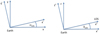Fig. B.1 Transformation from global coordinate system (z-axis pointing to zenith) to local coordinate system (x″ pointing along the LOS).

Rotation by the polar angle δ_LOS defines coordinate system F″, in which the galaxy’s unit vector is $${n^{″}}_x={n^{\prime }}_x\cos {\delta }_{LOS}+{n^{\prime }}_z\sin {\delta }_{LOS},$$(B.4) $${n^{″}}_y={n^{\prime }}_y,$$(B.5) $${n^{″}}_z=-{n^{\prime }}_{x}sin{\delta }_{LOS}+{n^{\prime }}_{z}cos{\delta }_{LOS}.$$(B.6)

In coordinate system F″, the $\widehat{x}\prime$-axis is directed along the LOS. The angular coordinates in F″ are $${\alpha }^{″}=\alpha -{\alpha }_{LOS},$$(B.7) $${\delta }^{″}={\sin }^{-1}\left({n^{″}}_z\right).$$(B.8)

Thus, Cartesian coordinates in the local coordinate system are defined as $$X=r\left(z\right){n^{″}}_x,$$(B.9) $$Y=r\left(z\right){n^{″}}_y,$$(B.10) $$Z=r\left(z\right){n^{″}}_z.$$(B.11)

References

All Figures

	Fig. 1 Cartoon illustrating the two-point correlation (0 – 1), three-point correlation (0 – 1 – 2), four-point correlation (0 – 1 – 2 – 3), and n-point correlation (0 – 1 – 2 – 3 – … - (n − 1)).
In the text

Fig. 2 Cartoon illustrating a three-point correlation (0 – 1 – 2) with different scales s1 on the side (0 – 1) and s2 on the side (0 – 2). Integration over spherical shells K1 and K2 is equivalent to counting all possible triangles that have one vertex at point 0 and the other two anywhere on the spheres. For the calculation of ${\xi }_3^{\text{iso}}\left(s_1,s_2\right)$, the kernels are uniformly populated, while for the evaluation of the Legendre expansion coefficients ${\xi }_3^{l_1,l_2}\left(s_1,s_2\right)$ they are populated with the values of $Y_{l_i{m}_i}\left(i=1,2\right)$. The values of mi are scanned from −li to +li, resulting in 2(2l + 1) convolutions for each value of l, since both real and imaginary parts of Ylm must be used.

In the text

	Fig. 3 Two-dimensional slices of spherical kernels, radius 108 h−1 Mpc, gS = 8 h−1 Mpc. The slices are transverse to the LOS direction moving outward (top to bottom). The value of kernel cells is shown for four configurations: l = 0, m = 0 (real); l = 2, m = 0 (real); l = 2, m = 1 (real); l = 2, m = 1 (imaginary).
In the text

	Fig. 4 Two-dimensional slices of spherical kernels, radius 108 h−1 Mpc, gS = 8 h−1 Mpc. The slices are along the LOS direction. The value of kernel cells is shown for three configurations corresponding to a complete wedge (0.0 < µ < 1.0), ξ⊥ (0.0 < µ < 0.5), and ξ∥ (0.5 < µ < 1.0).
In the text

	Fig. 5 ConKer flowchart. Parameters or settings chosen by the user are in blue, internal processes are in green, and decisions made by the user are in red.
In the text

Fig. 6 Execution time of the four processes in the ConKer algorithm, as applied to subsamples of the SDSS DR12 CMASS NGC galaxies (150° < αg < 210°, 0° < δg < 60°). Each point represents a calculation of the 2pcf (l = 0,2,4), 3pcf (l = 0–5), and diagonal npcf up to n = 5. Top: dependence on the number of combined data and random objects, using a grid resolution gS = 8 h−1 Mpc. Bottom: dependence on the grid resolution gS for 12.5M objects. The points represent the measured CPU time. The dashed lines are the results of the fit to a power law, with the scaling given in the figure. The solid line (bottom) is the time of the convolution step fit to $N_{\text{c}}^{4/3}\log N_{\text{c}}$.

In the text

Fig. 7 A comparison of the 2pcf as measured by the ConKer algorithm versus existing clustering algorithms. Top: 2pcf monopole ${\xi }_2^0\left(s\right)$ computed using ConKer with three different values of grid spacing gS = 8 (grey), 4 (blue), 2 (red) h−1 Mpc, and results from Cuesta et al. (2016) (purple line). Finer grids were resampled to ∆s = 8 h−1 Mpc bins. The error bars on the ConKer points were extracted from the covariance matrix of the Patchy mock ensemble. The errors in Cuesta et al. (2016; shaded region) are from an ensemble of quick particle mesh mocks (White et al. 2014). The 2pcf is multiplied by s2 to emphasize features at large scales. The lower subpanel shows the residual between the two methods. Bottom: same as the top panel, but for the 2pcf quadrupole ${\xi }_2^2\left(s\right)$. Here, the 2pcf is multiplied by s instead of s2 by convention.

In the text

Fig. 8 Points showing the transverse ξ⊥(s) and parallel ξ‖(s) components of the 2pcf computed using ConKer with three values of grid spacing gS = 8 (red–yellow), 4 (purple–green), 2 (black–grey) h−1 Mpc. Solid lines in the corresponding colors show the results from the nbodykit 2pcf algorithm. This figure corresponds only to NGC galaxies. The error bars and shaded regions are determined from the ensemble of Patchy mocks. The lower subpanels show the residual between the two methods.

In the text

Fig. 9 A comparison of the 3pcf estimated using ConKer compared to existing methods. Top: edge-corrected 3pcf, ${\xi }_3^l\left(s_1,s_2\right)$, computed using ConKer (left column) and nbodykit (right column) up to l = 3. The color scale is applicable to all panels. Bottom: residual between the two methods, shown as a distribution over all (s1, s2) pairs for l = 0 (blue), l = 1 (yellow), l = 2 (green), and l = 3 (red).

In the text

	Fig. 10 Angular footprint of the NGC (top) and SGC (bottom) galaxies (grey dots), divided into partitions (dashed red lines), each with a unique LOS (blue marker). The solid red line highlights one such partition. During the convolution step, the center of the kernel is positioned within these boundaries, while the convolution is performed over the region bound by the solid green line.
In the text

Fig. 11 Diagonal npcf, ξn(s), from n = 2 to n = 5 (from top to bottom), for the combined SGC+NGC sample of the ensemble of MD Patchy mocks (green) and the associated randoms (red dashed line). The shaded green region around the mock average gives the errors computed from the diagonal elements of the mock co-variance matrix, C. The npcf is multiplied by a proxy for the total kernel volume, where $\tilde{s}=s\text{/}\left(100h^{-1}\text{\hspace{0.17em}Mpc}\right)$. This convention highlights features at large scales.

In the text

	Fig. 12 Reduced covariance matrix $C_{ij}\text{/}\sqrt{C_{ii}{C}_{jj}}$ for the n = 2 diagonal isotropic correlation function. It is computed from the ensemble of Patchy mocks.
In the text

	Fig. 13 Three-point correlation function ${\xi }_3^l\left(s_1,s_2\right)$ of the NGC mock ensemble, computed up to l = 5. Multiplication by ${\tilde{s}}_1^2{\tilde{s}}_2^2$, emphasizes the same large-scale features as in Fig. 11. The diagonal elements are excluded from these plots.
In the text

	Fig. 14 Distribution, W0W1/⟨B0B1⟩ at s1 = 108 h−1 Mpc, for the CMASS galaxy sample of the SDSS DR12 survey (black), one of the MD Patchy mocks (green), and the associated randoms (red). This plot includes NGC galaxies only.
In the text

	Fig. B.1 Transformation from global coordinate system (z-axis pointing to zenith) to local coordinate system (x″ pointing along the LOS).
In the text

References

- Acquaviva, V., Bartolo, N., Matarrese, S., & Riotto, A. 2003, Nucl. Phys. B, 667, 119 [NASA ADS] [CrossRef] [Google Scholar]
- Bartolo, N., Komatsu, E., Matarrese, S., & Riotto, A. 2004, Phys. Rep., 402, 103 [NASA ADS] [CrossRef] [Google Scholar]
- Brown, Z., Mishtaku, G., Demina, R., Liu, Y., & Popik, C. 2021, A&A, 647, A196 [NASA ADS] [CrossRef] [EDP Sciences] [Google Scholar]
- Carron, J., & Neyrinck, M. 2012, ApJ, 750, 28 [NASA ADS] [CrossRef] [Google Scholar]
- Cuesta, A. J., Vargas-Magana, M., Beutler, F., et al. 2016, MNRAS, 457, 1770 [NASA ADS] [CrossRef] [Google Scholar]
- Cui, W., Liu, L., Yang, X., et al. 2008, ApJ, 687, 738 [NASA ADS] [CrossRef] [Google Scholar]
- DESI Collaboration (Aghamousa, A., et al.) 2016, The DESI Experiment Part I: Science, Targeting, and Survey Design [arXiv:1611.00036] [Google Scholar]
- Feldman, H. A., Kaiser, N., & Peacock, J. A. 1994, AJ, 426, 23 [NASA ADS] [CrossRef] [Google Scholar]
- Hamilton, A. J. S. 1993, ApJ, 417, 19 [Google Scholar]
- Hand, N. E. A. 2018, AJ, 156, 4 [Google Scholar]
- Jing, Y. 2005, ApJ, 620, 559 [NASA ADS] [CrossRef] [Google Scholar]
- Kitaura, F.-S., Rodríguez-Torres, S., Chuang, C.-H., et al. 2016, MNRAS, 456, 4156 [NASA ADS] [CrossRef] [Google Scholar]
- Landy, S. D., & Szalay, A. S. 1993, ApJ, 412, 64 [Google Scholar]
- Maldacena, J. M. 2003, JHEP, 05, 013 [NASA ADS] [CrossRef] [Google Scholar]
- March, W. B. 2013, Ph.D. Thesis, Georgia Institute of Technology, USA [Google Scholar]
- Meerburg, P.D., Green, D., Flauger, R., et al. 2019, BAAS, 51, 107 [NASA ADS] [Google Scholar]
- Philcox, O. H. E., Slepian, Z., Hou, J., et al. 2021, MNRAS, 509, 2457 [NASA ADS] [CrossRef] [Google Scholar]
- Portillo, S. K. N., Slepian, Z., Burkhart, B., Kahraman, S., & Finkbeiner, D. P. 2018, ApJ, 862, 119 [Google Scholar]
- Rodríguez-Torres, S. A., Chuang, C.-H., Prada, F., et al. 2016, MNRAS, 460, 1173 [CrossRef] [Google Scholar]
- Ross, A. J., Beutler, F., Chuang, C.-H., et al. 2017, MNRAS, 464, 1168 [Google Scholar]
- Sánchez, A. G., Scoccimarro, R., Crocce, M., et al. 2017, MNRAS, 464, 1640 [Google Scholar]
- Slepian, Z., & Eisenstein, D. J. 2015, MNRAS, 454, 4142 [NASA ADS] [CrossRef] [Google Scholar]
- Slepian, Z., & Eisenstein, D. J. 2016, MNRAS, 455, L31 [Google Scholar]
- White, M., Tinker, J. L., & McBride, C. K. 2014, MNRAS, 437, 2594 [NASA ADS] [CrossRef] [Google Scholar]
- Yuan, S., Eisenstein, D. J., & Garrison, L. H. 2018, MNRAS, 478, 2019 [NASA ADS] [CrossRef] [Google Scholar]
- Zhang, X., & Yu, C. 2011, Third IEEE International Conference on Cloud Computing Technology and Science, 634 [Google Scholar]
The python3 implementation of this algorithm can be downloaded at https://github.com/zbrown89/divide_conker
Technically, in this procedure each galaxy is counted twice, once when it is in the center cell and once when it is in the spherical shell, resulting in the overall factor of 2. However, since the same is also true for the random galaxies used for normalization, this factor cancels out.