| Issue |
A&A
Volume 667, November 2022
|
|
|---|---|---|
| Article Number | A147 | |
| Number of page(s) | 13 | |
| Section | Planets and planetary systems | |
| DOI | https://doi.org/10.1051/0004-6361/202141455 | |
| Published online | 21 November 2022 | |
SimAb: A simple, fast, and flexible model to assess the effects of planet formation on the atmospheric composition of gas giants
1
Anton Pannekoek Institute for Astronomy, University of Amsterdam,
Science Park 904,
1098XH
Amsterdam, The Netherlands
e-mail: This email address is being protected from spambots. You need JavaScript enabled to view it.
2
SRON Leiden,
Niels Bohrweg 4,
2333 CA
Leiden, The Netherlands
3
Space Research Institute, Austrian Academy of Sciences,
Schmiedlstrasse 6,
8042
Graz, Austria
4
SUPA, School of Physics & Astronomy, St Andrews University,
North Haugh, St Andrews
KY169SS, UK
5
Centre for Exoplanet Science, University of St Andrews,
North Haugh, St Andrews
KY169SS, UK
Received:
2
June
2021
Accepted:
21
December
2021
Abstract
Context. The composition of exoplanet atmospheres provides us with vital insight into their formation scenario. Conversely, planet formation processes shape the composition of atmospheres and imprint their specific signatures. In this context, models of planet formation containing key formation processes help supply clues to how planets form. This includes constraints on the metallicity and carbon-to-oxygen ratio (C/O ratio) of the planetary atmospheres. Gas giants in particular are of great interest due to the amount of information we can obtain about their atmospheric composition from their spectra, and also due to their relative ease of observation.
Aims. We present a basic, fast, and flexible planet formation model, called Simulating Abundances (SimAb), that forms giant planets and allows us to study their primary atmospheric composition soon after their formation.
Methods. In SimAb we introduce parameters to simplify the assumptions about the complex physics involved in the formation of a planet. This approach allows us to trace and understand the influence of complex physical processes on the formed planets. In this study we focus on four different parameters and how they influence the composition of the planetary atmospheres: initial protoplanet mass, initial orbital distance of the protoplanet, planetesimal ratio in the disk, and dust grain fraction in the disk.
Results. We focus on the C/O ratio and the metallicity of the planetary atmosphere as an indicator of their composition. We show that the initial protoplanet core mass does not influence the final composition of the planetary atmosphere in the context of our model. The initial orbital distance affects the C/O ratio due to the different C/O ratios in the gas phase and the solid phase at different orbital distances. Additionally, the initial orbital distance together with the amount of accreted planetesimals cause the planet to have subsolar or supersolar metallicity. Furthermore, the C/O ratio is affected by the dust grain fraction and the planetesimal ratio. Planets that accrete most of their heavy elements through dust grains will have a C/O ratio close to the solar C/O ratio, while planets that accrete most of their heavy elements from the planetesimals in the disk will end up with a C/O ratio closer to the C/O ratio in the solid phase of the disk.
Conclusions. By using the C/O ratio and metallicity together we can put a lower and upper boundary on the initial orbital distance where supersolar metallicity planets are formed. We show that planetesimals are the main source for reaching supersolar metallicity planets. On the other hand, planets that mainly accrete dust grains will show a more solar composition. Supersolar metallicity planets that initiate their formation farther than the CO ice line have a C/O ratio closer to the solar value.
Key words: planets and satellites: formation
© ESO 2022
1 Introduction
Over the past few decades different groups have addressed the question of whether the atmospheres of planets can provide any information on their formation histories. Mordasini et al. (2016) showed that the formation history of a planet affects the composition of the planetary atmosphere. Further studies show that the composition of the atmosphere of planets is affected by the composition of the disk (Öberg et al. 2011; Helling et al. 2014; Notsu et al. 2020). However, the composition of the disk can evolve over time. This evolution can affect the composition of the planets that are forming in these disks (Ali-Dib et al. 2014; Piso et al. 2016; Ilee et al. 2017; Booth & Ilee 2019). On the other hand, the processes that deliver solids to the planet forming envelope can play a considerable role in the composition. These processes can be either due to pebbles or planetesimals (Booth et al. 2017; Venturini et al. 2016; Pinhas et al. 2016; Voelkel et al. 2020). Additionally, Madhusudhan et al. (2014), showed that the composition of planetary atmospheres can provide us with information regarding the migration of the planet.
In recent years, advancements in observation techniques (Snellen et al. 2010; Otten et al. 2020; Brogi & Line 2019) have led to characterizations of exoplanet atmospheres, primarily hot Jupiters (e.g., Hoeijmakers et al. 2018; Helling et al. 2014; Kesseli & Snellen 2021; Serindag et al. 2021). In some of these studies the connection between the formation history of a planet and the observation of the planet atmosphere is addressed (Mollière et al. 2020; Giacobbe et al. 2021). In these studies they looked at the carbon-to-oxygen ratio (C/O ratio) in the atmosphere of HD 209456b and HR 8799e. Based on the C/O ratio of HD 209456b they suggest the planet is most likely formed farther than the H2O ice line and probably between the CO2 and CO ice lines. The C/O ratio and the individual abundances of the carbon and oxygen in HR 8799e suggest that the planet has accreted a solid mass between 65 and 360 Earth masses, and it is more likely for the planet to have initiated its formation beyond the CO ice line. Advancements in instrument precision and waveband coverage in the future with JWST and ARIEL (Tinetti et al. 2018) will make it possible to test and study the theories that have been developed and to validate the connections between the atmosphere composition to their formation history.
Of all the elements in exoplanet atmospheres, carbon, oxygen, and their ratio are some of the most widely studied, where important connections to a planet’s formation history have been drawn in various studies (Öberg & Bergin 2016; Cridland et al. 2016; Notsu et al. 2020). Further studies have delved into other elements, such as nitrogen (Bosman et al. 2019; Cridland et al. 2020; Turrini et al. 2021). These studies show that the nitrogen abundance in the giant planets can provide us with important information about the origin of planets that were formed beyond the CO snow line. Furthermore we can get information regarding the chemical evolution of the disk. Other studies have looked into the relative metallicity between a planet atmosphere and the host star and how the metallicity of the host star affects the metallicity of the planets (Thorngren et al. 2016; Santos et al. 2017; Hasegawa et al. 2019; Thiabaud et al. 2015). These studies show that there is a direct relation between the composition of the star and the planets; however, there is not a direct relationship between the C/O ratio of the planets and the metallicity of the hosting star.
The C/O ratio is a powerful tool for studying the composition of the planetary atmospheres because of its connection to the planet formation history and its relative ease in observation. Nonetheless, the C/O ratio alone cannot help us distinguish between the many processes that affect it, including but not limited to migration, the evolution of the disk, and the late enrichment of the atmosphere by planetesimals. Other markers must be used to untangle the history of the planet in combination with the C/O ratio.
In this study we construct a new way to look at planet formation that combines many vital processes together to form a gas giant planet. To do so, we bring the physical processes back to their essential form and dependences. This allows us to consider all dependences and parameterize unknown factors in the formation process. With SimAb1 we can perform large-scale parameter studies and eventually use it as retrieval and atmospheric analysis tools.
In Sect. 2 we discuss the basic assumptions. We describe how we set up the abundances in the disk in Sect. 2.1. In Sect. 2.2 we explain how we set up the disk module. In Sect. 2.3 we describe how the forming planet accretes gas and solid material from the disk. In Sect. 2.4 we explain how SimAb takes migration into account. In Sect. 3 we describe how the parameters were set up in this study. In Sect. 4 we describe the results of SimAb and how the input values can affect them. In Sect. 5 we discuss how our results in the context of previous studies can improve our understanding of how planet formation can be traced through the composition of the planetary atmospheres. Finally, in Sect. 6 we provide a summary of this study.
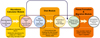 |
Fig. 1 Schematic showing how SimAb functions. SimAb has three main modules: the abundance module, the disk module, and the planet formation and migration module. The abundance module takes the total abundance of the disk and the condensation temperature of the most abundant molecules that each atom can form at each temperature. Then based on the integrated assumptions, SimAb calculates the dust-to-gas ratio and the abundances of the solid and gas for different temperatures with regard to the condensation temperatures. Additionally, the disk module calculates the disk temperature using a fixed dust-to-gas ratio and an alpha parameter, while it calculates the gas density using the dust-to-gas ratio that the abundance module calculates. The planet module takes the output of both the abundance module and the disk module together with the initial conditions of the protoplanetary core and calculates the mass and the composition of the planet based on a new dynamical alpha parameter to calculate the required migration rate to form the desired planet. |
2 Method
We constructed a planet formation simulation that takes planet core parameters, disk parameters, and the disk elemental abundances as input, and returns the planet atmospheric elemental abundances of a formed planet at a given orbital distance and a given mass. In this work we simulate the formation of gas giants assuming core accretion and Type II migration. By tracking the material the planet accretes, we track the atmospheric elemental abundances of planets. The simulation monitors the effects of the initial core mass, orbital separation, the dust grain fraction of the disk’s solid phase, and the planetesimal ratio.
SimAb is comprised of three main modules: a steady-state disk module, an abundance module, and a planet formation module. The overall structure of the method is depicted in Fig. 1. The disk module indicates the properties of the protoplanetary disk such as its temperature, density, and scale height. We use an abundance module to compute the abundance of the atoms in the solid and gas phase. The abundance calculator then calculates the dust-to-gas ratio based on how much material is in the solid phase at each temperature. The planet formation module computes how much mass is accreted onto the planet from the solid and gas phases of the disk. Moreover, the planet formation module calculates the migration distance due to Type II migration. In this simulation we adjust the migration speed by introducing a varying alpha parameter so the planet can reach the final orbital distance at the same time it reaches the desired mass. This allows us to form a planet with the same mass and orbital distance with various initial conditions. In the following sections we describe each of these modules and the assumptions therein.
Condensates used in our abundance module and their condensation temperatures.
2.1 Calculating the solid and gas abundances in the disk
The abundance module calculates the abundances of the different atoms in the solid and gas phases in the disk at a given temperature. Then, based on this composition, it calculates a dust-to-gas ratio. The values used in this study are not unique and there are many ways to deviate from the abundances assumed in this study. Therefore, our model allows the use of other abundances for the atoms in the gas and solid phase. This abundance would heavily affect the results and should be taken into account when studying the results. In this study we use certain assumptions for the abundances of the atoms in the disk which we explain in this section. The disk is assumed to have a solar composition following the reported values by Asplund et al. (2009). Furthermore, we assume that the condensation temperature is independent of the pressure and density in the disk. With these assumptions the module calculates the gas and solid abundance for each element for different temperatures in the disk. The atoms used in this work are presented in Table 1. We chose these atoms to keep the disk characterization simple and have a good variety of atoms for further studies on planetary atmospheres. The composition of the disk is known to follow a disequilibrium chemistry (Bergin et al. 2007). However, this is not true for a region close to the star within a few tenths of an AU. In this region the temperature and the density are higher; therefore, the composition can follow an equilibrium chemistry, following studies by Eistrup et al. (2018) and Öberg & Bergin (2021). In the inner region with a temperature of over 500 K, corresponding to a distance of 0.7 AU, we use condensate predicted by equilibrium chemistry for the temperatures and typical densities of this region. For temperatures lower than 500 K, we assume that atoms that are used to form refractories are all in the solid phase. Therefore, their abundances in the solid phase are the same as solar abundances. For other atoms, namely helium, carbon, and nitrogen, we use meteorite abundances reported by Asplund et al. (2009). The meteorite abundance in this study is water rich; therefore, we cannot separate the abundance of oxygen that was added because of water ice or other forms. Therefore, we assume the oxygen abundance at 500 K is the same as was calculated through the equilibrium chemistry. In order to determine how much hydrogen is in the solid phase we exclude the hydrogen abundance needed to form water from the hydrogen abundance that is reported in Asplund et al. (2009). At each ice line the condensed species abundance is added to the solid state abundances. Using the assumption in Öberg et al. (2011), we assume 15% of the remaining carbon is locked up in CO2 gas and the rest forms quickly into CO with the excess oxygen forming H2O.
In the hot region we use an approach similar to that mentioned in Min et al. (2011), assuming each atom forms a few main condensates (see Table 1). At each given temperature we first determine the main condensates in that temperature, and deplete all the atoms into those condensates with regard to the limiting atom. We use GG-chem (Woitke et al. 2018) to determine the main species formed for a wide range of pressures (101 to 10−6 bar) for temperatures above 500 K. The procedure of how the abundance module calculates the abundances of the solid using these abundances is explained in Table 1. This table is organized as a task list and shows how we remove elements from the gas phase at different temperatures. This process is not done based on the molecule condensation temperatures, but instead the molecules are sorted based on the abundance of their limiting atoms. As an example, for a temperature higher than 1100 K, first the magnesium and oxygen needed to form MgAl2O4 are removed from the gas phase. Then the magnesium and oxygen needed to form MgSiO3 are removed. This is to make sure at this temperature that all the aluminum is condensed in the solid phase. The abundance module then calculates the dust-togas ratio. Figure 2 shows the dust-to-gas ratio that the abundance module calculates. The increase in the dust-to-gas ratio is due to the condensation of the condensates mentioned in Table 1. Figure 3 shows the C/O ratio in the gas phase and the solid phase. The partition of carbon and oxygen is also presented in Table 2
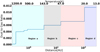 |
Fig. 2 Dust-to-gas ratio calculated by abundance module based on the amount of atoms in the solid and gas phase. This plot shows how the dust-to-gas ratio changes throughout the disk. The steps in the plot are caused by the condensation of different species mentioned in Table 1. The colors in the plot indicate different regions in the disk. Cyan indicates region A, and shows the disk within the water ice line. Black indicates region B, and shows the disk farther than the water ice line and within the CO2 ice line. Red indicates region C, and shows the disk between the CO2 ice line and CO ice line. Blue indicates region D, and shows the disk farther than the CO ice line. |
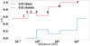 |
Fig. 3 C/O ratio over the disk in the gas phase and solid phase. The C/O ratio starts as a solar value in the gas phase, closer to the star. By condensation of Al2O3, at point 1, Mg2SiO4 at point 2, and KAlSi3O8 and NaAlSi3 O8 at point 3, the C/O ratio increases in the gas phase. Due to the lack of carbon in the solid phase for these steps, the C/O ratio is zero until point 4 where part of the carbon is condensed to form a meteorite-like composition. This results in a decrease in the C/O ratio in the gas phase. At point 5 the condensation of H2O increases the C/O ratio in the gas phase. At point 6 CO2 condenses into ice. This increases the C/O ratio in the gas phase up to 1. Finally at point 7, by condensing CO, the C/O ratio becomes solar in the solid phase. The gas phase at this point is oxygen and carbon free. |
Partition of carbon and oxygen in the disk.
2.2 Disk module
We assume a one-dimensional disk based on the analytical model represented in Min et al. (2011). The temperature is calculated assuming viscous heating in the inner regions where the disk is optically thick. For the regions where the temperature dominates by the irradiation of the star, we use the temperature reported in Ida et al. (2016). Equations (1) and (2) show the viscosity and irradiation temperature, respectively. The disk temperature is the maximum value of these two temperatures. Equation (3) calculates the density of the mid-plane:
![Mathematical equation: ${T^5} = {{3\mu {m_{\rm{p}}}\dot M} \over {3{\pi ^2}\alpha {k_{\rm{p}}}f\sigma }}{\left[ {{{G{M_*}} \over {{R^3}}}} \right]^{3/2}},$](/articles/aa/full_html/2022/11/aa41455-21/aa41455-21-eq1.png) (1)
(1)
 (2)
(2)
 (3)
(3)
In these equations µ is the mean molecular mass of the gas, mp is the proton mass,  is the mass accretion rate of the star, α is the viscosity constant, and
  is the dust-to-gas ratio. The dust-togas ratio varies between 0.01 and 0.004 depending on the atomic abundance of the solid and gas in the disk. We use a constant dust-to-gas ratio of 0.01 to calculate the temperature and a varying dust-to-gas ratio for the solid condensation. We assume that the planet is formed in a short time compared to the disk evolution so the star mass accretion rate as well as the ice line positions are constant during the planet formation, following Eistrup et al. (2018).
In addition to the temperature and density, the disk module calculates the scale height of the disk H, the speed of sound cs, and the angular velocity at the given orbital distance.
2.3 Planet module
The planet module forms a gas giant planet through a core accretion model. In SimAb we assume each single simulation forms a single planet. Since we are interested in the atmospheric composition of the planets, SimAb starts the formation after the protoplanet core is formed and starts the runaway gas accretion. Furthermore, we assume the protoplanet mass is higher than the pebble isolation mass. For simplicity, the planets formed go through Type II migration throughout the time they accrete their atmospheres. The model is set with the assumption that migration and gas accretion halt simultaneously when the planet reaches the desired mass and orbital distance.
The planet module calculates the composition of the atmosphere of planets and the mass of material accreted through the solid phase and the gas phase. It also adjusts the migration speed of the planet so that the planet reaches the required mass and orbital distance at once.
2.3.1 Gas accretion
In SimAb the planet formation starts by assuming a core of a few Earth masses starting runaway gas accretion. We assume this mass is already larger than the pebble isolation mass.
We use Bitsch et al. (2019) to calculate the accreted gas onto the planet. Equation (4) shows the rate at which the planet accretes mass. The planet gas accretion rate is restricted by the Bondi accretion rate (Ida & Lin 2004) and the viscous flux of the disk. In Eq. (4), the first part calculates the viscous flux and the result is equal to the star mass accretion, while the second part is the Bondi rate.
 (4)
(4)
The accreted gas consists of volatile material as well as some refractories in the form of dust grains. These grains are small enough that they are fully coupled to the gas and move around with the gas. The composition of the gas then depends on the dust-to-gas ratio as well as how much of the solid is in the form of dust grains, the dust grain fraction. In the case where all the material is in the form of dust, the dust grain fraction is one, the composition of the accreted gas would be solar. The abundance module calculates the dust-to-gas ratio that we use in this step for each given temperature. The densities of the gas and solids that we use in this step are given in Fig. 4. The gas accretion stops once the planet reaches its final orbital distance which happens at the same time that the planet reaches its final mass.
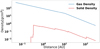 |
Fig. 4 Density change of the gas and the solid at different orbital distances. The steps in the solid density are caused by the different dust-to-gas ratios at different orbital distances. |
2.3.2 Solid accretion
The solid component of the disk is defined by four parameters. The first parameter is the dust-to-gas ratio,  , which indicates what fraction of the disk mass is in solids. We introduce the dust grain fraction, δdust, as the second parameter; the pebble fraction, δpebbie, as the third; and the planetesimal fraction, δpls, as the last. These last three parameters are smaller than one and together add up to one. A ratio of zero defines a situation where there is either no dust, no pebbles, or no planetesimals in the system (depending on which solid fraction has a ratio of zero) and a value of one represents the opposite case where the system is comprised solely of dust, pebbles, or planetesimals (depending on which solid has a fraction of one). In order to keep the model simple, we assume the solid fractions, δpls and δpebble, are the same throughout the disk.
We assume that the starting core mass in our simulation is higher than the pebble isolation mass, and therefore the planet does not accrete pebbles. On the other hand, the simulation recognizes accretion of dust grains and planetesimals.
Dust grains have a Stokes number much lower than one, are coupled to the gas, and are accreted through runaway gas accretion. The dust grain mass accreted via runaway gas accretion is determined by the dust-to-gas ratio,  , and by the dust grain fraction, δdstg. Equation (5) calculates the dust mass present in the accreted gas mass, Macc,g:
 (5)
(5)
Planetesimals are defined as objects with a Stokes number much higher than one and that have diameters of a few to a few hundred kilometers. Planetesimals are not much affected by gas drag, and even after the gap opening planets can accrete planetesimals. We assume that the planetesimals are spread throughout the disk with the same distribution as the gas density. The dynamical interaction between the planet and the planetesimals is ignored. The planet accretes planetesimals present in its feeding zone, which we define as one Hill radius around the planet. However, for the purpose of our study the exact radius of the feeding zone does not matter as the planet will eventually accrete a fixed ratio of planetesimals in the area that it sweeps through during its formation, єpls. The planetesimal fraction, δpls, and the efficiency in accreting planetesimals, єpls can vary independently. The product of these two values is called the planetesimal ratio, δє,pls, and is shown in Eq. (6). Equation (7) shows the increase in planet mass by accreting planetesimals:
 (6)
(6)
 (7)
(7)
In this equation Σg is the gas density and δє,pls is the planetesimal ratio. The planetesimals are dissolved in the atmosphere and the remaining mass reaching the surface of the planet core is negligible (Podolak et al. 1988; Pollack et al. 1996; Venturini et al. 2016).
The planetesimal composition is dependent on the formation region; therefore, SimAb allows for different assumptions for the planetesimal composition. In this study we adjust the composition of the planetesimals to the composition of the solids at the distance they are accreted.
2.4 Migration and evolution
SimAb assumes the planet is only going through Type II migration with an inward direction through the disk. The migration stops when the planet reaches its final orbital distance, which is given as an input in the initial parameters. This assumption allows us to have an estimate of the composition of the planet without overly complicating the model.
We implement migration using the migration rate from Alibert et al. (2005), shown in Eq. (8):
 (8)
(8)
Here, αd is the dynamical viscous constant of the disk, Ω is the angular velocity of the disk, rp is the planet orbital distance, mp is the planet mass, and Σg is the gas density. The value of αd can vary between 10−6 for very low viscosity disks and less than 1 for high viscosity disks. Varying α allows us to change the migration timescale and match it to the formation timescale of the planet. This assumption allows us to reproduce the formation of hot and ultrahot giant planets from small cores starting as far as 250 AU or form planets in situ.
The migration rate is slower once the mass of the gas within the planetary orbit is less than the planet mass; however, we assume the same migration rate, even when the planet mass is heavier than the disk mass within its orbit. This assumption allows us to adjust the model in a way so that all the formed planets can end in the same spot, without affecting their accretion rate. Using an accretion rate that is dependent on the planet mass would interact with the computational aspect of the model, which forces the planet to finish its formation at the same orbital distance and mass, and would force the planet to accrete the majority of its mass in situ. We discuss the impact of such a simplification in Sect. 5.
SimAb is not robust against non-physical αd values with values greater than one. For αd values close to one some of the assumptions we make are no longer valid. Even though focusing on such planets is beyond the scope of this study, such values would allow the prediction of planets formed with a similar composition that must have migrated through methods aside from just disk viscosity migration.
Variable input parameters and their ranges.
Fixed input parameters of the model.
3 Setting up the variables
We run simulations for a hundred and thirty thousand different initial conditions to form a Jupiter-mass planet at 0.02 AU. There are four main parameters governing the formation of these planets, the initial orbital distance and the initial core mass, the dust grain fraction, and the planetesimal ratio. The last two parameters describe the solid size distribution. The planetesimal ratio also contains information about the efficiency of the planets in accreting planetesimals.
The boundaries of these input parameters are given in Table 3. The initial orbital distance cannot be closer to the star than the final orbital distance because the model does not support outward migration. The planet cannot start its runaway gas accretion at the same distance as the final orbital distance because the migration step size must be greater than zero. The initial mass can vary between 5 and 30 Earth masses (Piso et al. 2015; Piso & Youdin 2014). We assume that the dust grain fraction and the planetesimal ratio are constant throughout the disk. The value of the other variables that we use in the model are given in Table 4.
4 Results
We ran simulations for a hundred thousand different initial conditions following the above procedure to form a Jupiter-mass planet at a distance of 0.02 AU. An additional 30 thousand runs were performed where the initial orbital distances were chosen from a uniform distribution within the CO2 ice line in order to populate the samples in the regions within this ice line. The calculated C/O ratio versus metallicity of the formed planets from these runs are plotted in Fig. 5. The plot uses four different colors to encode the starting distance of the planet embryo. The metallicities of planetary atmospheres that we report in this work only include the atoms we trace in SimAb and do not trace other atoms and are expressed in units of solar metallicity on a log scale. Moreover, the core composition does not contribute to the metallicity of the planets in this work.
Figures 6–8 show how each of these regions is affected by the four main parameters. In the following paragraphs we explain these plots.
Figure 6 consists of four subplots. These subplots show the C/O ratio versus metallicity of the atmosphere of the planets that SimAb produces. Each of the subplots is a zoom-in on a different region that was introduced in Fig. 5.
The color bar in these plots indicates the initial mass of the protoplanets. The initial core mass varies between 5 and 35 Earth masses. This plot shows that the composition of the planets does not have a clear correlation with the initial mass of the protoplanets. There is a lack of correlation between the initial mass and the composition of the planets because the metallicity and the C/O ratio are both affected by the amount of solids that the planet accretes. SimAb takes into account two ways to accrete solids onto the atmosphere: accretion of dust grains in the gas and accretion of planetesimals. The amount of dust grains in the gas is governed by the dust-to-gas ratio and how much solid mass is in the form of dust grains in the disk. On the other hand, in this model the solid mass accreted through planetesimals does not depend on the initial mass of the planet.
Figure 7 shows the relation between the composition of the planets, the C/O ratio and metallicity, and the initial orbital distance of the protoplanet. Each subplot shows planets that initiated their formation in a different region. In this figure the color bar shows the initial orbital distance of the protoplanet core. All the subplots show a clear correlation between the composition of the planet atmosphere, mainly the C/O ratio, and where the planet initiates its formation. However, depending on the region in which the planet initiates its formation, these correlations have different characteristics. In order to understand why this relation changes for different regions, we look at the planets with subsolar metallicity and supersolar metallicity separately for these regions. The reason for this approach is that planets with subsolar metallicity accrete most of their atmosphere mass from the gas phase of the disk, while planets with supersolar metallicity accrete a more substantial mass from the solid phase. Figure 3 shows the C/O ratio variations as a function of distance from the star, for both the solid phase and the gas phase in the disk. For planets with subsolar metallicity we need to focus on the C/O ratio of the gas phase in the disk. For supersolar metallicity planets, we need to mainly focus on the C/O ratio of the solid phase in the disk.
In the top left subplot, which is a zoom-in on planets initiating their migration from region A in Fig. 5, the C/O ratio decreases as the planet’s initial orbital distance increases. All of this region lies in the subsolar metallicity half of the C/O— metallicity plot. By looking at the C/O ratio in the gas phase for distances within the water ice line we see the C/O ratios increase for a short distance up to 0.7 AU. When the carbonaceous material condenses, this value decreases in the gas phase. Therefore, planets that initiate their formation beyond 0.7 AU accrete part of their mass from a gas with a lower C/O ratio. The farther out they initiate their formation, the more mass they accrete with a lower C/O ratio compared to planets initiating their formation at closer distances.
Planets that initiate their formation beyond the water ice line can have both supersolar and subsolar metallicity. We first focus on the planets with subsolar metallicity. In region B the C/O ratio in the gas phase increases due to the condensation of the water into its icy form. Therefore, planets that mainly accrete from the gas phase will end up with an increasing C/O ratio as their initiating distance increases. On the other hand, those planets that have a supersolar metallicity tend to have a decreasing C/O ratio as well as increasing metallicity when increasing their starting distance from the star.
In region C, beyond the CO2 ice line and within the CO ice line, we see that for the planets with the same metallicity, those that initiate their formation farther out have a higher C/O ratio. This is expected as the C/O ratio in this region increases in the solid phase and the gas phase. Hence, regardless of the phase of the material a planet accretes in this region, the farther out a planet initiates its formation, the more material it accretes with a higher C/O ratio compared to the inner regions. Planets with supersolar metallicity, migrating from within this region, tend to have a lower C/O ratio as their metallicity increases. These planets tend to accrete more from the solid phase and their C/O ratio approaches the C/O ratio in the solid phase.
Beyond the CO ice line, all the carbon and oxygen will be in the solid phase. In this region the solid phase will have a solar C/O ratio, while the gas phase is fully depleted from oxygen and carbon. Therefore, the C/O ratio of the planets that mainly accrete gas is largely influenced by the C/O ratio in the gas phase within the CO ice line. Figure 3 shows that the C/O ratio in the gas phase within the CO ice line is always supersolar, consequently the C/O ratio of such planets will be supersolar. On the other hand, planets that accrete a high mass from the solid phase (when the accreted solid mass to the accreted gas mass is higher than the dust-to-gas ratio of the disk) will end up with a subsolar to slightly supersolar C/O ratio. This is true because the C/O ratio in the solid phase is subsolar everywhere in the disk within the CO ice line, and is solar beyond the CO ice line. The farther out the planet initiates its formation, the more solids it can accrete with a solar C/O ratio. As a result, planets that initiate formation farther away from the star will have a C/O ratio closer to the solar value.
Figure 8 shows the relation between the C/O ratio and the metallicity of the atmosphere of the planets to the amount of solid mass that the planet accretes in the form of dust grains. The plot consists of four subplots which are oriented in the same way as the previous plots. The color bar in these subplots shows how much dust is available for the planet to accrete, yellow for disks where the majority of the solid material is in dust grain form, and dark blue for disks where there is not much dust available.
The top left subplot, showing protoplanets that migrated from region A, shows a very strong correlation between the C/O ratio and metallicity and the amount of dust grains accreted onto the planet. The planets that are formed in disks with a higher abundance of dust are more likely to have a solar composition. On the other hand, planets that are formed beyond the CO2 ice line do not show as much correlation. Nevertheless, planets that are formed in a disk with a high dust grain fraction tend to have a C/O ratio and a metallicity closer to solar compared to planets that are formed in disks where not much dust is available. As planets in this model accrete gas and dust simultaneously, in the extreme case where the dust grain fraction is one the accreted material and thus the atmosphere of such planets will have a solar composition. This explains why increasing the amount of dust in the natal disk causes the formed planet to have a more solar composition.
In Fig. 9, as in the previous plots, we plotted the C/O ratio versus the metallicity of the formed planets. The color bar in these plots shows the overall efficiency of accreting planetesimals and how many planetesimals are available for the formation of each planet. Planets that are shown in yellow are assumed to be very efficient in accreting planetesimals and are formed in disks with a high fraction of solid mass being in planetesimal form. On the other hand, planets that are shown in darker colors are formed in disks with few planetesimals and or are not very efficient in accreting them. This plot shows that planets that are formed within the water ice line, region A, behave differently compared to those that initiate their formation beyond the CO2 ice line, regions C and D. The composition of these planets is mainly affected by the dust grain fraction, and the accreted planetesimals would not affect the composition. The correlation that we see in this plot comes mainly from the assumption that the summation of planetesimal fraction together with the dust grain fraction cannot acquire a value higher than one. Planets that initiate their formation within the water ice line show a weaker correlation between their composition, the C/O ratio and metallicity, and the planetesimal ratio. On the other hand, planets that are formed farther than the CO2 ice line show a very strong correlation with the planetesimal ratio. Planets that are formed beyond the CO2 ice line show a higher metallicity as their efficiency in accreting planetesimal increases. They generally show a lower C/O ratio compared to planets that are formed at the same distance. To understand the behavior of the composition of the planets regarding their efficiency in accreting planetesimals for those planets that are formed in region B, we need to understand at what distance the accretion of planetesimals can dominate the heavy element abundance in the planetary atmosphere.
Figure 10 shows the metallicity of planets that SimAb forms compared to the distance where these planets initiate their formation. Planets that are shown in blue are Jupiter-mass planets at a distance of 0.02 AU, while planets in orange have five Jupiter masses and are at the same orbital distance. This plot shows that heavier planets acquire lower metallicities compared to less massive planets when initiating their formation at the same distance. Hence, in order to form a heavy planet with supersolar metallicity, it must form farther out compared to a less massive planet. In addition to this, planets that are more efficient in accreting dust grains tend to have solar metallicity, as demonstrated by Fig. 8, while planets that accrete more planetesimals end up with higher metallicity, as shown in Fig. 9. From all this we can conclude that heavier planets need to accrete a higher mass in the form of planetesimals compared to less massive planets in order for their metallicity to be supersolar.
Figure 11 shows how much mass can be accreted in the form of planetesimals based on where the planet initiates its migration. In this plot we assume that the planet final orbital distance is at 0.02 AU. In this plot we indicated the distances at which planets with one and five Jupiter masses can initiate their formation in order to have supersolar metallicity. For a planet composition to be affected by the planetesimal accretion, the ratio of total mass accreted in planetesimals to the total gas mass of the planet must be higher than the maximum dust-to-gas ratio of where the planet accretes its material. In this model the region with the maximum dust-to-gas ratio coincides with the region where the planet initiates its formation.
Comparing Figs. 11 and 10 we see that at distances of 7.8 AU, which is where a Jupiter-mass planet with supersolar metallicity can originate from, and 31.7 AU, where a five Jupiter-mass planet with supersolar metallicity can originate from, the total mass in the form of planetesimals that a forming planet can accrete are respectively 1.45 Earth masses and 9.75 Earth masses. The total mass that would contribute to the metallicity thus comes from the heavy elements accreted through the gas, dust grains, and the planetesimals. Comparing this to how much mass these planets accrete from the gas phase, we see that the ratio of the planetesimal mass to the gas mass must be 0.0046 for a Jupiter-mass planet at 7.75 AU, and 0.0061 for a five Jupiter-mass planet at 31.7 AU. These are similar values to the dust-to-gas ratio at the distance of 7.8 AU and 31.7 AU. Planets that can accrete enough mass from the solid phase so that the dust-to-gas ratio becomes higher than that in a disk with solar composition will have a supersolar metallicity. In this model this is only achievable by accreting planetesimals as the dust grain can at most bring the metallicity of the planet as high as solar. In other words, for a planet to have a supersolar metallicity it must accrete more solid mass in the form of planetesimals than it can through dust grains. Knowing this, we can put a lower limit on where a supersolar metallicity planet should have initiated its formation based on how massive the planet is.
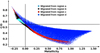 |
Fig. 5 C/O ratio and the log scale of metallicity of 100 thousand planets with one Jupiter mass at a distance of 0.02 AU with different compositions. The different compositions are caused by the different formation initial conditions (see Sect. 3). The four different colors show planets that initiated their formation in four different regions of the disk. Cyan indicates planets that initiated their migration within the water ice line, region A. Black indicates planets that initiated their migration farther than the water ice line and within the CO2 ice line, region B. Red indicates planets that initiated their migration beyond the CO2 ice line and within the CO ice line, region C. Blue indicates planets that initiated their migration farther than the CO ice line, region D. |
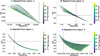 |
Fig. 6 C/O ratio and the log scale metallicity of the planets formed by the model and presented in Fig. 5. The color bar indicates the initial core mass of these planets. Shown are zoom-ins on the four regions explained in Fig. 5. The top left panel shows planets that initiate their formation in region A, the top right panel shows planets that initiate their formation in region B, the bottom left panel shows planets that initiate their formation in region C, and the bottom right panel shows planets that initiated their migration from region D. In all four panels there is no clear correlation between the C/O ratio and the metallicity of the planetary atmospheres and their initial core mass. |
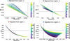 |
Fig. 7 C/O ratio and the log scale metallicity of the planets formed by SimAb and presented in Fig. 5. The color bar indicates the initial core orbital distances of these planets. Shown are zoom-ins on the four regions explained in Fig. 5. Top left panel: planets that initiate their formation in region A; in this region the planets that initiate their formation farther out would end up with a lower C/O ratio. Top right panel: planets that initiate their formation in region B; in this region planets with subsolar metallicity that are formed farther out have higher C/O ratios. Additionally, only planets that are formed closer to the CO2 ice line show supersolar metallicity. Bottom left panel: planets that initiate their formation in region C; given planets with the same metallicity, planets that initiate their formation farther out have a higher C/O ratio. Bottom right panel: planets that initiate their formation in region D; planets with supersolar metallicity show C/O ratios closer to the solar value as the planet initiates its formation farther out. Planets with supersolar metallicity can reach higher metallicities when initiating their formation farther out. |
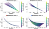 |
Fig. 8 C/O ratio and the log scale metallicity of the planets formed by SimAb and presented in Fig. 5. The color bar indicates the dust grain fraction. Shown are zoom-ins on the four regions explained in Fig. 5. In all four plots the planets that are formed in disks with higher dust grain fractions show metallicity and a C/O ratio closer to the solar value. This relation becomes less strong for planets that initiate their formation in farther regions, such as region C and D. |
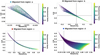 |
Fig. 9 C/O ratio and the log scale metallicity of the planets formed by SimAb presented in Fig. 5. The color bar indicates the planetesimal ratio. Shown are zoom-ins on the four regions explained in Fig. 5. Planets that initiate their formation in region A in disks with higher planetesimal ratio, show lower metallicity and a higher C/O ratio. On the other hand, planets that initiate their formation in regions B, C, or D show a very strong correlation with the planetesimal ratio. Planets that initiate their formation in these regions with a high planetesimal ratio show a higher metallicity and a lower C/O ratio. In all four plots the planets that are formed in disks with higher dust grain fractions show metallicities and C/O ratios closer to the solar value. This relation becomes less strong for planets that initiate their formation in farther regions, such as regions C and D. |
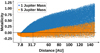 |
Fig. 10 Log scale metallicity and initial orbital distance of planets of one Jupiter mass (blue) and five Jupiter masses (orange) at an orbital distance of 0.02 AU. This plot shows that planets with five Jupiter masses need to initiate their formation farther out compared to planets with one Jupiter mass in order to have a supersolar metallicity. The dashed lines show the initial orbital distances at which these planets start showing supersolar metallicity. |
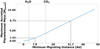 |
Fig. 11 Maximum mass that can be accreted through planetesimals for a planet that finishes its migration at a distance of 0.02 AU. The x-axis shows the minimum initial orbital distance where the planet starts its migration and the y-axis shows the maximum possible accreted mass in the form of planetesimals. The vertical lines show the different ice lines in the disk. The vertical dashed lines show the distances where a planet with one and five Jupiter masses can initiate its migration in order to have a supersolar metallicity. The horizontal dashed lines show the amount of planetesimal mass that a planet can accrete by initiating its migration at the indicated distances. |
5 Discussion
In this work we introduced SimAb, a planet formation model based on a simple planet formation scenario and studied how different initial conditions of the model would affect the final composition of the planetary atmosphere. We investigated the effect of four parameters, the initial protoplanet mass, the initial protoplanet orbital distance, the dust grain fraction, and the planetesimal ratio.
We find that the C/O ratios and metallicities of exoplanet atmospheres are affected by three of the four parameters investigated in the model (initial orbital distance of the protoplanet, the dust grain fraction, and the planetesimal ratio). However, we find that the initial core mass has no influence on the final C/O ratio or metallicity, as seen in Fig. 6.
Additionally, we find that this model predicts that the C/O ratio does not provide enough information to retrieve any of the four parameters. In order to estimate any of these planet formation parameters, we find that at least one other observable parameter must be included, such as the metallicity of the atmosphere of the planets, in order to accurately determine any parameters in a planet formation history.
5.1 Metallicity
In this work we show that metallicity is a powerful tool and can inform us about the initial orbital distance for supersolar metallicity planets where the planet starts its runaway gas accretion. We confirm that giant planets can achieve supersolar metallicity by accreting planetesimals during the rapid gas accretion phase which is in agreement with previous studies done by Thorngren et al. (2016) and Turrini et al. (2021). Furthermore, we show that the main source of metallicity is the accretion of planetesimals. This result is also supported by Mordasini et al. (2016). Moreover, Podolak et al. (2020) and Turrini et al. (2021) show that planetesimal accretion plays an important role during the rapid gas accretion phase.
In this work we confirm that there is a relation between the distance a planet migrates and its metallicity. The greater the distance a planet migrates, the more planetesimals it can accrete. This is in agreement with previous works such as Shibata et al. (2020) and Turrini et al. (2021). Our results show a relation between the mass of the planet, its metallicity, and the distance a planet needs to migrate in order to reach a certain metallicity which is in agreement with previous studies (Thorngren et al. 2016; Mordasini et al. 2016; Shibata et al. 2020). Additionally, Madhusudhan et al. (2014) showed that planets that go through disk migration have a supersolar metallicity. This is in agreement with the result of this study. However, Madhusudhan et al. (2014) showed that planets that initiate their formation very far out in the disk cannot go through disk migration. Therefore, they will have very low metallicity.
5.2 C/O ratio
In this work we show that as long as the solid phase and the gas phase stays oxygen rich the planet atmosphere will be oxygen rich. This is in agreement with Mordasini et al. (2016). In our study, no planet with a C/O ratio higher than 1 is formed because the C/O ratio of the disk does not reach any value higher than 1 in this model. This explains the differences we see in the C/O ratio between our study and other studies such as Mordasini et al. (2016) and Turrini et al. (2021). Madhusudhan et al. (2014) showed that planets that are formed very far out can achieve supersolar C/O ratios. Our results on the other hand show that planets formed at any distance can have a supersolar C/O ratio. This happens because the C/O ratio in the gas phase in all regions is supersolar. On the other hand, planets that initiate their formation farther out and accrete planetesimals can have a subsolar C/O ratio because the solid phase in the disk is subsolar in the model. It is worth mentioning that the C/O ratio in this study is heavily influenced by the initial assumptions about the oxygen and carbon carriers. If we use other abundances for the ice species or include other carriers such as organic compounds, the planets can acquire different C/O ratios (Eistrup et al. 2018; Öberg & Bergin 2021).
5.3 Metallicity–C/O plane
An important outcome of this run of SimAb is shown in Fig. 5, which reveals that formed planets are primarily found in two opposite areas: those with a supersolar C/O ratio and subsolar metallicity, and those with a subsolar C/O ratio and supersolar metallicity. This result was previously shown in Madhusudhan et al. (2014) and Turrini et al. (2021). This outcome was expected, and is a direct consequence of our assumptions of how the abundances change in the disk. Nevertheless, this is interesting because the metallicity of the formed planets is essentially affected by planetesimal accreted through planet migration in this model.
Migration significantly increases the availability of planetesimal accretion. Consequently, planets with subsolar metallicities mainly formed from gas accretion from the disk, whereas planets with supersolar metallicity were polluted by the solids that accreted during the migration phase. Therefore, for subsolar compositions a comparison to the gas phase is appropriate. However, for supersolar compositions it is important to investigate the C/O ratio of the solids that have been accreted during migration.
Planets can acquire higher metallicities if they accrete enough planetesimals, such that the ratio between the planetesimal mass accreted and the total mass of the planet becomes higher than the maximum dust-to-gas ratio of the accreted gas. This provides a lower boundary on the orbital distance where a planet with supersolar metallicity could have initiated its formation.
We can also place boundaries on the C/O ratio based on where a planet starts its formation, as seen in Fig. 7. As an example, a planet that initiates its formation at 12 AU can only have a C/O ratio between 0.5 and 0.7. In this range the lower boundary of the C/O ratio is acquired by planets that are more efficient in accreting solids, while the upper limit is acquired by a planet that mainly accretes gas. It is important to keep in mind that in Fig. 7 we show the maximum possible mass in the form of planetesimals that a planet can accrete by migrating from a certain distance. Shibata et al. (2020) and Turrini et al. (2021) show on the other hand that planets do not accrete all the planetesimals in a disk therefore this approach can determine a minimum distance from where a planet can accrete enough solid mass to achieve a certain metallicity. Using other information about the composition of the planets such as the C/O ratio, we can determine how efficient a planet is in accreting solids.
Comparing the C/O ratio of a planet to the minimum and maximum C/O ratio possible at each initial orbital distance in Fig. 7 informs us about how efficient the planet is in accreting solids when combined with information on its metallicity. For planets with supersolar metallicity, its metallicity gives information on the closest orbital distance where the planet could have initiated its formation. For these planets the C/O ratio gives information on how efficient the accretion of solids or gas is. Lower efficiency in accreting solids thus indicates that the planet must have formed farther out than the minimum orbital distance suggested by its metallicity. The combination of the two is thus a powerful tool to trace initial orbital distances for supersolar metallicity planets.
However, this approach is not as robust for planets with subsolar metallicity. For these planets we need to compare the metallicity of the planet with the metallicity of the gas in the disk. The metallicity in the disk decreases for larger orbital distance; therefore, lower metallicities are possible for planets that initiate their gas accretion farther out. In planets with subsolar metallicity, the heavy element abundance is affected by both the dust grain fraction and the composition of the disk in the gas and solid phase. By increasing the dust grain fraction to unity, the planet will end up accreting a solar composition from the disk regardless of the solid and gas composition. However, for lower values of dust grain fraction, knowing the ratio between the amount of solid and gas accreted from the disk can help us determine the effects on the composition caused by accreting mass from different regions. In such cases, it becomes much more important to have a clear idea of the ratio between the mass accreted from the solid phase and the gas phase. Therefore, it is better to look at another composition indicator in the atmosphere. Possible indicators could be S/N, Si/N, Fe/N, or Mg/N because sulfur, silicon, iron, and magnesium are mostly found in the solid phase, while the majority of the nitrogen in the disk stays in the gas phase except where the temperature is below 18 K. Hence, these elements are better indicators of how much solid and gas are accreted than just carbon and oxygen (Turrini et al. 2021). This study suggests that lower Si/N or Mg/N would indicate a higher rate of gas accretion compared to solid accretion, and a higher Si/N or Mg/N would indicate the opposite.
5.4 Limitations of SimAb and future work
In this section we go over the limitations of SimAb, how our assumptions can affect the results and what are our plans for the future to improve these limitations.
The first assumption we make is to assume the material accreted onto the planet after the planet initiates its Type II migration dominates the observable atmosphere of the mature planet. This reduces the number of processes that we include in the model and only focuses on the impact that Type II migration can have on the composition of the atmosphere. However, more detailed study is needed to compare the impact of different aspects of planet formation, such as Type I migration, and of early enrichment of the planetary envelope, as is discussed in Helled et al. (2014). It is also important to take care of the different triggering masses, such as the relation between pebble isolation mass and the runaway gas accretion mass, as these masses can vary due to different aspects of the disk and the forming planet. Venturini et al. (2016) suggested that the pebble isolation mass is higher at greater orbital distances, while Helled et al. (2014) and Venturini & Helled (2017) discuss different aspects of the disk that can result in varying masses to trigger runaway gas accretion such as how polluted the envelope around a forming planet is. Including these considerations may result in a composition different from what SimAb predicts for gas giants.
The other assumption concerning the initial core mass is that the starting core masses are between 5 and 35 Earth masses. However, the mass of the protoplanet cores in regions farther out need to be much higher than a few Earth masses in order to be able to initiate runaway gas accretion. This means some of the simulated planets in this work might not be able to form as the initial core mass is too low. As we show in Fig. 6, the initial core mass does not impact the results we report in this work; therefore, this inconsistency does not impact our results.
In addition to the source of the heavy elements, whether it is due to the accretion of planetesimals or pebbles, their composition is very important. Larger bodies can lock some icy material in them and have them at distances closer than the ice lines. This means that even planets that are formed in the close-in regions can have C/O ratios similar to planets that are formed farther out. Even though SimAb is flexible in its use of different compositions for larger solid bodies, we made the assumption that the composition of the solids accreted onto the planet varies by temperature. This would not affect how we estimate the initial orbital distance of the protoplanet, but would affect the range of distances at which a protoplanet might start forming as a gas giant.
The third assumption is that accreted planetesimals are fully dissolved into the atmosphere of the forming planets. Even though this is a valid assumption for planets with large and thick atmospheres, this is not necessarily correct for planets with smaller and thinner atmospheres. This means that in the early stages of formation the metallicity of the planet can stay intact, even though the mass of the planet increases due to the accretion of the planetesimals. The composition of the planets that are formed in region C may have lower metallicities and higher C/O ratios. Planets with supersolar metallicity that are formed in region D, on the other hand, would have lower C/O ratios (Fig. 5).
Another assumption is that the planet initiates a Type II migration as soon as it starts accreting its atmosphere. The planet migrates throughout the formation process, and the migration stops once the atmosphere accretion halts. However, we know that planets can accrete gas even before they start Type II migration (Ida & Lin 2004). This means that the planet can already have a thin atmosphere composed of the gas and dust in the surrounding area before it starts to migrate. This can affect the composition of the planetary atmosphere. These planets can eventually have a composition more similar to the disk at the orbital distance where they initiate their formation. In addition, planets can migrate outward; however, for this study we only implement an inward motion for the planets, and there could be pebble accretion; other processes that are not accounted for could also change the final composition of the planets. These processes are beyond the scope of the current paper.
SimAb only takes into account the orbital change due to Type II migration. As mentioned in Alibert et al. (2005), when the planet mass becomes higher than the mass of the disk within its orbit, its migration rate will be a fraction of the migration rate otherwise. However, we assume that the migration rate follows the same equation. Hence, the planets that are formed move faster than is predicted for them once they reach this boundary. This means that in this model planets would move faster through the inner regions than is predicted, which skews their composition toward the compositions of the outer regions. If the model instead slowed down the protoplanet in the final region, we would see possibly unrealistic compositions that are almost fully determined by the inner region compositions, due to how the time spent in each region influences what material and how much material is accreted in the model, which primarily affects the C/O ratio. This does not influence the metallicity of the planets as it would not affect the amount of planetesimals accreted onto the planets.
Another assumption that we want to discuss is on the accretion of planetesimals. We assume that the planetesimal ratio is a constant value. However, this may not be the case. There are different dynamical influences from the planet on the planetesimals that can change the amount of accreted planetesimals throughout its formation. Shibata et al. (2020) looked into these dynamical effects in great detail. Furthermore, Turrini et al. (2021) shows that the efficiency of accreting planetesimals varies throughout the disk. As we discussed earlier, the composition of the planetesimals and the amount of accreted planetesimals are important. Nonetheless, the metallicity of the planet can put a maximum limit on the maximum dust-to-gas ratio of the disk that was accreted onto the planet and provide a minimum orbital distance where the planet initiates its formation.
One of the assumptions in this study is the composition of the disk. This assumption has a significant impact on our results. However, SimAb allows for different elemental abundances as well as additional ices in the disk. By including new atoms and elements, SimAb can assist us in tracing new atmospheric observations back to the planet formation. Moreover, we can study the impact of disk composition on the composition of the planet atmosphere. Nitrogen is one of the elements that SimAb can allow us to study. As we mentioned in Sect. 5.3, nitrogen can give us insight into the planet formation history. Additionally, nitrogen can affect the oxygen and carbon partition in the disk (Eistrup et al. 2018).
6 Conclusion
We built SimAb, a simple planet formation model, to study the composition of planetary atmospheres. In this work we used a two-stage chemistry for the disk, an equilibrium chemistry region for hotter regions and a disequilibrium chemistry region for the cooler regions. The abundance calculator module includes CO2, CO, and H2O ice lines. We assumed that the planet is going through runaway gas accretion and accretes heavy elements either through planetesimal accretion or the dust grains that are coupled to the gas. We parameterized the formation scenario to be able to study the effect of different parameters of the formation. The parameters we used are the atomic abundances of the disk, host star properties, distribution of the solids in the disk, information about the planet, and viscosity of the disk. In this work we fixed the star and the atomic abundances in the disk; however, we studied the impact of solid distribution in the disk, the initial orbital distance, and mass of the protoplanet. We used the viscosity as an indirect variable to ensure that we formed the same planet by running different initial conditions. The conclusion of this work can be summarized as follows:
The metallicity and the C/O ratio (composition) of the formed planets are only moderately dependent on the initial core mass.
Planetesimals are the main source of heavy elements for planets with supersolar metallicity.
Planets that are mainly accreting dust grains show a solar value for their metallicity and their C/O ratio, regardless of the distance at which they initiate their formation.
Metallicity and the C/O ratio together can put restrictions on where the planet initiates its formation. Planets that are formed farther than CO ice line tend to show solar values for the C/O ratio when they accrete more planetesimals.
These results are compatible with previous studies (see Sect. 5) while providing freedom to analyze the impact of various assumptions about the planets and their environment on the atmospheric composition of the planet.
Acknowledgments
J.M.D. acknowledges support from the Amsterdam Academic Alliance (AAA) Program, and the European Research Council (ERC) European Union’s Horizon 2020 research and innovation program (grant agreement no. 679633; Exo-Atmos). This work is part of the research program VIDI New Frontiers in Exoplanetary Climatology with project number 614.001.601, which is (partly) financed by the Dutch Research Council (NWO). P. W. acknowledges funding from the European Union H2020-MSCA-ITN-2019 under Grant Agreement no. 860470 (CHAMELEON). We thank Alex Cridland, Douglas Lin, Melissa McClure, Christoph Mordasini, and Chris Ormel for the various discussions that contributed to this work.
References
- Alibert, Y., Mordasini, C., Mousis, O., & Benz, W. 2005, Space Sci. Rev., 116, 77 [NASA ADS] [CrossRef] [Google Scholar]
- Ali-Dib, M., Mousis, O., Petit, J.-M., & Lunine, J. I. 2014, ApJ, 785, 125 [NASA ADS] [CrossRef] [Google Scholar]
- Asplund, M., Grevesse, N., Sauval, A. J., & Scott, P. 2009, Ann. Rev. Astron. Astrophys., 47, 481 [CrossRef] [Google Scholar]
- Bergin, E. A., Aikawa, Y., Blake, G. A., & van Dishoeck, E. F. 2007, in Protostars and Planets V, eds. B. Reipurth, D. Jewitt, & K. Keil (Tucson: University of Arizona Press), 751 [Google Scholar]
- Bitsch, B., Izidoro, A., Johansen, A., et al. 2019, A&A, 623, A88 [NASA ADS] [CrossRef] [EDP Sciences] [Google Scholar]
- Booth, R. A., & Ilee, J. D. 2019, MNRAS, 487, 3998 [CrossRef] [Google Scholar]
- Booth, R. A., Clarke, C. J., Madhusudhan, N., & Ilee, J. D. 2017, MNRAS, 469, 3994 [Google Scholar]
- Bosman, A. D., Cridland, A. J., & Miguel, Y. 2019, A&A, 632, L11 [NASA ADS] [CrossRef] [EDP Sciences] [Google Scholar]
- Brogi, M., & Line, M. R. 2019, AJ, 157, 114 [Google Scholar]
- Cridland, A. J., Pudritz, R. E., & Alessi, M. 2016, MNRAS, 461, 3274 [Google Scholar]
- Cridland, A. J., van Dishoeck, E. F., Alessi, M., & Pudritz, R. E. 2020, A&A, 642, A229 [NASA ADS] [CrossRef] [EDP Sciences] [Google Scholar]
- Eistrup, C., Walsh, C., & van Dishoeck, E. F. 2018, A&A, 613, A14 [NASA ADS] [CrossRef] [EDP Sciences] [Google Scholar]
- Giacobbe, P., Brogi, M., Gandhi, S., et al. 2021, Nature, 592, 205 [NASA ADS] [CrossRef] [Google Scholar]
- Hasegawa, Y., Hansen, B. M. S., & Vasisht, G. 2019, ApJ, 876, L32 [NASA ADS] [CrossRef] [Google Scholar]
- Helled, R., Bodenheimer, P., Podolak, M., et al. 2014, Protostars and Planets VI (Tucson: University of Arizona Press) [Google Scholar]
- Helling, C., Woitke, P., Rimmer, P., et al. 2014, Life, 4, 142 [NASA ADS] [CrossRef] [Google Scholar]
- Hoeijmakers, H. J., Ehrenreich, D., Heng, K., et al. 2018, Nature, 560, 453 [CrossRef] [Google Scholar]
- Ida, S., & Lin, D. N. C. 2004, ApJ, 604, 388 [Google Scholar]
- Ida, S., Guillot, T., & Morbidelli, A. 2016, A&A, 591, A72 [NASA ADS] [CrossRef] [EDP Sciences] [Google Scholar]
- Ilee, J. D., Forgan, D. H., Evans, M. G., et al. 2017, MNRAS, 472, 189 [NASA ADS] [CrossRef] [Google Scholar]
- Kesseli, A. Y., & Snellen, I. A. G. 2021, ApJ, 908, L17 [Google Scholar]
- Madhusudhan, N., Amin, M. A., & Kennedy, G. M. 2014, ApJ, 794, L12 [Google Scholar]
- Min, M., Dullemond, C. P., Kama, M., & Dominik, C. 2011, Icarus, 212, 416 [Google Scholar]
- Mollière, P., Stolker, T., Lacour, S., et al. 2020, A&A, 640, A131 [Google Scholar]
- Mordasini, C., van Boekel, R., Mollière, P., Henning, T., & Benneke, B. 2016, ApJ, 832, 41 [Google Scholar]
- Notsu, S., Eistrup, C., Walsh, C., & Nomura, H. 2020, MNRAS, 499, 2229 [Google Scholar]
- Öberg, K. I., & Bergin, E. A. 2016, ApJ, 831, L19 [Google Scholar]
- Öberg, K. I., & Bergin, E. A. 2021, Phys. Rep., 893, 1 [Google Scholar]
- Öberg, K. I., Murray-Clay, R., & Bergin, E. A. 2011, ApJ, 743, L16 [Google Scholar]
- Otten, G. P. P. L., Vigan, A., Muslimov, E., et al. 2020, A&A, 646, A150 [Google Scholar]
- Pinhas, A., Madhusudhan, N., & Clarke, C. 2016, MNRAS, 463, 4516 [NASA ADS] [CrossRef] [Google Scholar]
- Piso, A.-M.A., & Youdin, A.N. 2014, ApJ, 786, 21 [NASA ADS] [CrossRef] [Google Scholar]
- Piso, A.-M.A., Youdin, A.N., & Murray-Clay, R.A. 2015, ApJ, 800, 82 [NASA ADS] [CrossRef] [Google Scholar]
- Piso, A.-M.A., Pegues, J., & öberg, K.I. 2016, ApJ, 833, 203 [NASA ADS] [CrossRef] [Google Scholar]
- Podolak, M., Pollack, J. B., & Reynolds, R. T. 1988, Icarus, 73, 163 [NASA ADS] [CrossRef] [Google Scholar]
- Podolak, M., Haghighipour, N., Bodenheimer, P., Helled, R., & Podolak, E. 2020, ApJ, 899, 45 [NASA ADS] [CrossRef] [Google Scholar]
- Pollack, J. B., Hubickyj, O., Bodenheimer, P., et al. 1996, Icarus, 124, 62 [NASA ADS] [CrossRef] [Google Scholar]
- Santos, N. C., Adibekyan, V., Dorn, C., et al. 2017, A&A, 608, A94 [NASA ADS] [CrossRef] [EDP Sciences] [Google Scholar]
- Serindag, D. B., Nugroho, S. K., Mollière, P., et al. 2021, A&A, 645, A90 [EDP Sciences] [Google Scholar]
- Shibata, S., Helled, R., & Ikoma, M. 2020, A&A, 633, A33 [NASA ADS] [CrossRef] [EDP Sciences] [Google Scholar]
- Snellen, I. A. G., de Kok, R. J., de Mooij, E. J. W., & Albrecht, S. 2010, Nature, 465, 1049 [Google Scholar]
- Thiabaud, A., Marboeuf, U., Alibert, Y., Leya, I., & Mezger, K. 2015, A&A, 580, A30 [NASA ADS] [CrossRef] [EDP Sciences] [Google Scholar]
- Thorngren, D. P., Fortney, J. J., Murray-Clay, R. A., & Lopez, E. D. 2016, ApJ, 831, 64 [NASA ADS] [CrossRef] [Google Scholar]
- Tinetti, G., Drossart, P., Eccleston, P., et al. 2018, Exp. Astron., 46, 135 [NASA ADS] [CrossRef] [Google Scholar]
- Turrini, D., Schisano, E., Fonte, S., et al. 2021, ApJ, 909, 40 [Google Scholar]
- Venturini, J., & Helled, R. 2017, ApJ, 848, 95 [NASA ADS] [CrossRef] [Google Scholar]
- Venturini, J., Alibert, Y., & Benz, W. 2016, A&A, 596, A90 [NASA ADS] [CrossRef] [EDP Sciences] [Google Scholar]
- Voelkel, O., Klahr, H., Mordasini, C., Emsenhuber, A., & Lenz, C. 2020, A&A, 642, A75 [NASA ADS] [CrossRef] [EDP Sciences] [Google Scholar]
- Woitke, P., Helling, C., Hunter, G. H., et al. 2018, A&A, 614, A1 [NASA ADS] [CrossRef] [EDP Sciences] [Google Scholar]
All Tables
All Figures
|
Fig. 1 Schematic showing how SimAb functions. SimAb has three main modules: the abundance module, the disk module, and the planet formation and migration module. The abundance module takes the total abundance of the disk and the condensation temperature of the most abundant molecules that each atom can form at each temperature. Then based on the integrated assumptions, SimAb calculates the dust-to-gas ratio and the abundances of the solid and gas for different temperatures with regard to the condensation temperatures. Additionally, the disk module calculates the disk temperature using a fixed dust-to-gas ratio and an alpha parameter, while it calculates the gas density using the dust-to-gas ratio that the abundance module calculates. The planet module takes the output of both the abundance module and the disk module together with the initial conditions of the protoplanetary core and calculates the mass and the composition of the planet based on a new dynamical alpha parameter to calculate the required migration rate to form the desired planet. |
| In the text | |
|
Fig. 2 Dust-to-gas ratio calculated by abundance module based on the amount of atoms in the solid and gas phase. This plot shows how the dust-to-gas ratio changes throughout the disk. The steps in the plot are caused by the condensation of different species mentioned in Table 1. The colors in the plot indicate different regions in the disk. Cyan indicates region A, and shows the disk within the water ice line. Black indicates region B, and shows the disk farther than the water ice line and within the CO2 ice line. Red indicates region C, and shows the disk between the CO2 ice line and CO ice line. Blue indicates region D, and shows the disk farther than the CO ice line. |
| In the text | |
|
Fig. 3 C/O ratio over the disk in the gas phase and solid phase. The C/O ratio starts as a solar value in the gas phase, closer to the star. By condensation of Al2O3, at point 1, Mg2SiO4 at point 2, and KAlSi3O8 and NaAlSi3 O8 at point 3, the C/O ratio increases in the gas phase. Due to the lack of carbon in the solid phase for these steps, the C/O ratio is zero until point 4 where part of the carbon is condensed to form a meteorite-like composition. This results in a decrease in the C/O ratio in the gas phase. At point 5 the condensation of H2O increases the C/O ratio in the gas phase. At point 6 CO2 condenses into ice. This increases the C/O ratio in the gas phase up to 1. Finally at point 7, by condensing CO, the C/O ratio becomes solar in the solid phase. The gas phase at this point is oxygen and carbon free. |
| In the text | |
|
Fig. 4 Density change of the gas and the solid at different orbital distances. The steps in the solid density are caused by the different dust-to-gas ratios at different orbital distances. |
| In the text | |
|
Fig. 5 C/O ratio and the log scale of metallicity of 100 thousand planets with one Jupiter mass at a distance of 0.02 AU with different compositions. The different compositions are caused by the different formation initial conditions (see Sect. 3). The four different colors show planets that initiated their formation in four different regions of the disk. Cyan indicates planets that initiated their migration within the water ice line, region A. Black indicates planets that initiated their migration farther than the water ice line and within the CO2 ice line, region B. Red indicates planets that initiated their migration beyond the CO2 ice line and within the CO ice line, region C. Blue indicates planets that initiated their migration farther than the CO ice line, region D. |
| In the text | |
|
Fig. 6 C/O ratio and the log scale metallicity of the planets formed by the model and presented in Fig. 5. The color bar indicates the initial core mass of these planets. Shown are zoom-ins on the four regions explained in Fig. 5. The top left panel shows planets that initiate their formation in region A, the top right panel shows planets that initiate their formation in region B, the bottom left panel shows planets that initiate their formation in region C, and the bottom right panel shows planets that initiated their migration from region D. In all four panels there is no clear correlation between the C/O ratio and the metallicity of the planetary atmospheres and their initial core mass. |
| In the text | |
|
Fig. 7 C/O ratio and the log scale metallicity of the planets formed by SimAb and presented in Fig. 5. The color bar indicates the initial core orbital distances of these planets. Shown are zoom-ins on the four regions explained in Fig. 5. Top left panel: planets that initiate their formation in region A; in this region the planets that initiate their formation farther out would end up with a lower C/O ratio. Top right panel: planets that initiate their formation in region B; in this region planets with subsolar metallicity that are formed farther out have higher C/O ratios. Additionally, only planets that are formed closer to the CO2 ice line show supersolar metallicity. Bottom left panel: planets that initiate their formation in region C; given planets with the same metallicity, planets that initiate their formation farther out have a higher C/O ratio. Bottom right panel: planets that initiate their formation in region D; planets with supersolar metallicity show C/O ratios closer to the solar value as the planet initiates its formation farther out. Planets with supersolar metallicity can reach higher metallicities when initiating their formation farther out. |
| In the text | |
|
Fig. 8 C/O ratio and the log scale metallicity of the planets formed by SimAb and presented in Fig. 5. The color bar indicates the dust grain fraction. Shown are zoom-ins on the four regions explained in Fig. 5. In all four plots the planets that are formed in disks with higher dust grain fractions show metallicity and a C/O ratio closer to the solar value. This relation becomes less strong for planets that initiate their formation in farther regions, such as region C and D. |
| In the text | |
|
Fig. 9 C/O ratio and the log scale metallicity of the planets formed by SimAb presented in Fig. 5. The color bar indicates the planetesimal ratio. Shown are zoom-ins on the four regions explained in Fig. 5. Planets that initiate their formation in region A in disks with higher planetesimal ratio, show lower metallicity and a higher C/O ratio. On the other hand, planets that initiate their formation in regions B, C, or D show a very strong correlation with the planetesimal ratio. Planets that initiate their formation in these regions with a high planetesimal ratio show a higher metallicity and a lower C/O ratio. In all four plots the planets that are formed in disks with higher dust grain fractions show metallicities and C/O ratios closer to the solar value. This relation becomes less strong for planets that initiate their formation in farther regions, such as regions C and D. |
| In the text | |
|
Fig. 10 Log scale metallicity and initial orbital distance of planets of one Jupiter mass (blue) and five Jupiter masses (orange) at an orbital distance of 0.02 AU. This plot shows that planets with five Jupiter masses need to initiate their formation farther out compared to planets with one Jupiter mass in order to have a supersolar metallicity. The dashed lines show the initial orbital distances at which these planets start showing supersolar metallicity. |
| In the text | |
|
Fig. 11 Maximum mass that can be accreted through planetesimals for a planet that finishes its migration at a distance of 0.02 AU. The x-axis shows the minimum initial orbital distance where the planet starts its migration and the y-axis shows the maximum possible accreted mass in the form of planetesimals. The vertical lines show the different ice lines in the disk. The vertical dashed lines show the distances where a planet with one and five Jupiter masses can initiate its migration in order to have a supersolar metallicity. The horizontal dashed lines show the amount of planetesimal mass that a planet can accrete by initiating its migration at the indicated distances. |
| In the text | |
Current usage metrics show cumulative count of Article Views (full-text article views including HTML views, PDF and ePub downloads, according to the available data) and Abstracts Views on Vision4Press platform.
Data correspond to usage on the plateform after 2015. The current usage metrics is available 48-96 hours after online publication and is updated daily on week days.
Initial download of the metrics may take a while.