| Issue |
A&A
Volume 666, October 2022
|
|
|---|---|---|
| Article Number | A17 | |
| Number of page(s) | 21 | |
| Section | Extragalactic astronomy | |
| DOI | https://doi.org/10.1051/0004-6361/202243708 | |
| Published online | 29 September 2022 | |
Supermassive black holes at high redshift are expected to be obscured by their massive host galaxies’ interstellar medium
1
INAF – Osservatorio di Astrofisica e Scienza dello Spazio di Bologna, Via P. Gobetti 93/3, 40129 Bologna, Italy
e-mail: roberto.gilli@inaf.it
2
Department of Physics and Astronomy, Johns Hopkins University, Baltimore, MD 21218, USA
3
Space Telescope Science Institute, 3700 San Martin Drive, Baltimore, MD 21218, USA
4
Department of Physics and Astronomy, Clemson University, Kinard Lab of Physics, Clemson, SC 29634, USA
5
Institut de Ciències del Cosmos (ICCUB), Universitat de Barcelona (IEEC-UB), Martí i Franquès, 1, 08028 Barcelona, Spain
6
ICREA, Pg. Lluís Companys 23, 08010 Barcelona, Spain
7
Dipartimento di Fisica e Astronomia, Università degli Studi di Bologna, Via P. Gobetti 93/2, 40129 Bologna, Italy
8
SISSA, Via Bonomea 265, 34136 Trieste, Italy
9
INAF – Istituto di Radioastronomia, Via P. Gobetti 101, 40129 Bologna, Italy
10
Institut d’Astrophysique de Paris, 98bis Boulevard Arago, 75014 Paris, France
Received:
4
April
2022
Accepted:
18
July
2022
We combine results from deep ALMA observations of massive (M* > 1010 M⊙) galaxies at different redshifts to show that the column density of their interstellar medium (ISM) rapidly increases toward early cosmic epochs. Our analysis includes objects from the ASPECS and ALPINE large programs, as well as individual observations of z ∼ 6 quasar hosts. When accounting for non-detections and correcting for selection effects, we find that the median surface density of the ISM of the massive galaxy population evolves as ∼(1 + z)3.3. This means that the ISM column density toward the nucleus of a z > 3 galaxy is typically > 100 times larger than locally, and it may reach values as high as Compton-thick at z ≳ 6. Remarkably, the median ISM column density is on the same order of what is measured from X-ray observations of large active galactic nucleus (AGN) samples already at z ≳ 2. We have developed a simple analytic model for the spatial distribution of ISM clouds within galaxies, and estimate the total covering factor toward active nuclei when obscuration by ISM clouds on the host scale is added to that of parsec-scale circumnuclear material (the so-called torus). The model includes clouds with a distribution of sizes, masses, and surface densities, and also allows for an evolution of the characteristic cloud surface density with redshift, Σc, * ∝ (1 + z)γ. We show that, for γ = 2, such a model successfully reproduces the increase in the obscured AGN fraction with redshift that is commonly observed in deep X-ray surveys, both when different absorption thresholds and AGN luminosities are considered. Our results suggest that 80–90% of supermassive black holes in the early Universe (z > 6 − 8) are hidden to our view, primarily by the ISM in their hosts. We finally discuss the implications of our results and how they can be tested observationally with current and forthcoming facilities (e.g., VLT, E-ELT, ALMA, and JWST) and with next-generation X-ray imaging satellites. By extrapolating the observed X-ray nebulae around local AGN to the environments of supermassive black holes at high redshifts, we find ≲1″ nebulae impose stringent design constraints on the spatial resolution of any future X-ray imaging Great Observatory in the coming decades.
Key words: galaxies: ISM / galaxies: evolution / galaxies: high-redshift / quasars: supermassive black holes
© R. Gilli et al. 2022
 Open Access article, published by EDP Sciences, under the terms of the Creative Commons Attribution License (https://creativecommons.org/licenses/by/4.0), which permits unrestricted use, distribution, and reproduction in any medium, provided the original work is properly cited.
This article is published in open access under the Subscribe-to-Open model. Subscribe to A&A to support open access publication.
1. Introduction
Deep X-ray observations of the Universe have shown that most supermassive black holes (SMBHs) at galaxy centers grow hidden by dust and gas (see, e.g., Hickox & Alexander 2018 for a review) and that the incidence of obscuration in active galactic nuclei (AGN) strongly increases with redshift (La Franca et al. 2005; Treister & Urry 2006; Liu et al. 2017; Lanzuisi et al. 2018; Vito et al. 2018; Iwasawa et al. 2020). This is especially true for intrinsically luminous systems, as the fraction of quasars (QSOs) with Lbol ≳ 1045 erg s−1 (LX > 1044 erg s−1) that are obscured by hydrogen column densities of NH > 1023 cm−2 rises from 10–20% in the local Universe to ∼80% at z ∼ 4, when the Universe was only 1.5 Gyr old (Vito et al. 2018). The origin of this trend is not yet understood.
Indirect arguments suggest that the observed increase may not be linked to the incidence of small-scale obscuration at different cosmic epochs, that is, in the physical and geometric properties of the circumnuclear medium surrounding the nucleus that is often associated with the torus of dusty gas postulated by the unified models (see Netzer 2015 and Ramos Almeida & Ricci 2017 for recent reviews). Remarkably, the broadband spectral energy distributions (SEDs) of UV-bright QSOs look the same across cosmic time (Richards et al. 2006; Leipski et al. 2014; Bianchini et al. 2019). These SEDs include a prominent rest-frame near-IR bump produced by dust heated to T ∼ 1000 − 1500 K by the QSO UV radiation field and distributed on a-few-parsec scales around the nucleus (Netzer 2015). The QSO near-IR to UV luminosity ratio is a measure of the dust covering factor, which is on the order of 30–50% (Lusso et al. 2013). The self-similarity of QSO SEDs across cosmic time suggests that this ratio is constant with redshift, and so consequently is the covering factor of the circumnuclear dusty gas.
Other arguments suggest instead that the increased obscuration with redshift might occur on the host galaxy scale (≲kpc). The physical properties of the interstellar medium (ISM) in galaxies change rapidly with cosmic time. Empirical trends are being measured in several samples of star-forming galaxies spanning a broad redshift range, where the amount of cold gas, which contains most of the ISM mass, is seen to rapidly grow toward early cosmic time (Scoville et al. 2017; Tacconi et al. 2018; Aravena et al. 2020), possibly as fast as Mgas ∼ (1 + z)2 (Scoville et al. 2017). At the same time, galaxies have been observed to become progressively smaller at high redshifts, with typical size decreasing as r ∼ (1 + z)−1 (Allen et al. 2017). It then seems unavoidable that the ISM density rapidly grows toward early cosmic epochs, possibly as fast as ρgas ∼ Mgas/r3 ∼ (1 + z)5. Similarly, the column density of the ISM, NH, gas ∼ Mgas/r2, may grow as fast as ∼(1 + z)4, reaching values of 1023 cm−2 or even Compton-thick (NH > 1/σT ∼ 1.5 × 1024 cm−2, where σT is the Thomson cross section) in the distant Universe, where large, Mgas ∼ 1010 M⊙ ISM reservoirs have been observed in compact galaxies of characteristic size 1–2 kpc (see, e.g., Hodge & da Cunha 2020 for a recent review on distant, star-forming galaxies). In massive galaxies, the ISM is metal-rich (Lequeux et al. 1979; Tremonti et al. 2004; Maiolino et al. 2008), and such column densities would absorb the X-ray nuclear radiation very effectively, adding to the obscuration produced by the small-scale circumnuclear medium. By using Atacama Large Millimeter Array (ALMA) observations of a z = 4.75 Compton-thick QSO in the Chandra deep field south (CDFS), Gilli et al. (2014) find the ISM column density measured in this source to be comparable with the absorption to the nucleus measured from the X-ray spectrum. The same analysis was then expanded to a small sample of distant, obscured AGN in the redshift range z ∼ 2.5 − 4.7 by Circosta et al. (2019) and D’Amato et al. (2020), who also find a good correspondence between the level of nuclear absorption measured in the X-rays (∼1023 − 24 cm−2) and the ISM column density measured through ALMA data.
Numerical simulations also suggest that the ISM column density in distant galaxies is substantial (Trebitsch et al. 2019; Ni et al. 2020; Lupi et al. 2022). For example, Ni et al. (2020) find that, in the early Universe, z > 7, the ISM column density and covering factor of galaxy nuclei are so large that 99% of early SMBHs in their simulated galaxies grow hidden by gas column densities of NH > 1023 cm−2.
This work focuses on galaxies with stellar masses M* > 1010 M⊙, as: (i) they are the hosts of active SMBHs detectable in deep X-ray surveys up to the highest redshifts (Lanzuisi et al. 2017; Yang et al. 2017), and (ii) despite the overall decrease in galaxy metallicity with redshift, in such massive systems the ISM metallicity remains close to solar even at z ∼ 2 (Maiolino et al. 2008; Maiolino & Mannucci 2019) and drops to only ≲0.5× solar at z > 4 according to simulations (Torrey et al. 2019). We recall that, in the literature, solar metallicities and abundances are usually assumed to convert the column density of metals estimated through X-ray spectroscopy of large AGN samples into a total gas (hydrogen) column density (Tozzi et al. 2006; Lanzuisi et al. 2017; Liu et al. 2017; Vito et al. 2018). In massive galaxies, the comparison between the ISM-based and X-ray-based column densities is then fair. We use sensitive ALMA observations to determine the column density toward the nuclei of galaxies in samples at different redshifts. We then derive the cosmological evolution of the average ISM column density toward galaxy nuclei and of the fraction of ISM-obscured AGN, and compare with observations from deep X-ray surveys.
The paper is organized as follows. In Sect. 2 we present the ALMA galaxy samples used in this work. In Sect. 3 we describe the methodology adopted to derive gas masses and sizes for the galaxies in our samples. In Sect. 4 we work out a simple model to estimate the ISM column density toward galaxies’ nuclei and to quantify the cosmic evolution of the ISM-obscured AGN fractions. In Sect. 5 we present our main results on the cosmic evolution of the ISM column density. In Sect. 6 we discuss our findings, add the contribution of a small-scale torus to our ISM obscuration model, and compare our results with the fractions of obscured AGN observed in different X-ray samples. We also compare our findings with expectations from numerical simulations and finally present some possible observational diagnostics to test the proposed ISM-obscuration scenario. We draw our conclusions in Sect. 7. We also note in Sects. 6 and 7 significant design constraints on future X-ray imaging Great Observatories that are consequences of this work.
A concordance cosmology with H0 = 70 km s−1 Mpc−1, Ωm = 0.3, and ΩΛ = 0.7, in agreement within the errors with the Planck 2015 results (Planck Collaboration XIII 2016), is used throughout this paper. All stellar masses in the considered galaxy samples were originally computed using the Chabrier (2003) initial mass function (IMF).
2. Galaxy samples
We searched for samples of galaxies with M* > 1010 M⊙ featuring deep ALMA far-infrared (FIR)/millimeter observations. We require a continuum root mean square (rms) smaller than a few tens of μJy in band 6 or 7 (∼1.2 mm and ∼850 μm, respectively). These bands are commonly used for dust observations as they maximize the ALMA observing efficiency by targeting wavelengths close to the redshifted FIR SED peak of distant galaxies. The required rms allows us to probe dust masses down to ≈107 M⊙ at all redshifts (see Fig. 1), corresponding to ISM masses down to a few ×109 M⊙ (see next sections), and to detect > 50% of massive galaxies. A large FIR/millimeter detection rate is indeed key to perform any reliable correction for those systems missed by ALMA, likely poorer in gas, and hence to derive a sensible value for the average ISM density of the entire massive galaxy population. For objects at z > 4, the [C II]157.74 μm fine structure emission line is redshifted at ≳800 μm, where the atmosphere is relatively transparent and allows effective observations with ALMA. As the [C II] line is a major coolant for cold (T ≲ 300 K) gas (Wolfire et al. 2003) and one of the brightest emission lines in star-forming galaxies (Stacey et al. 1991, 2010), we use it to probe the ISM content of distant galaxies in addition to dust emission. The main samples considered in this work are described below and summarized in Table 1 sorted by increasing redshift. The source selection criteria at the basis of these samples are admittedly not homogeneous, nonetheless we compiled a large, “best-effort” collection of galaxies with sufficiently good data to determine their ISM column density. In Sect. 5.2, we try to correct a posteriori for the main selection biases and, in turn, draw general conclusions for the whole population of massive galaxies.
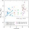 |
Fig. 1. Estimated dust mass vs. redshift for the considered galaxy samples as labeled. For high-z QSO hosts, dust masses have been estimated from Eq. (2) assuming Td = 47 K if Tmin < 47 K or Td = 1.2Tmin if Tmin > 47 K (see text for details). For the ASPECS and COSMOS samples, the original dust masses derived through SED-fitting (MAGPHYS) are plotted as open symbols, and those derived from a single MBB with Td = 47 K as filled symbols. The dashed curve shows the dust mass limit corresponding to a flux density of 30 μJy at 1.2 mm (i.e., the ∼3σ detection limit in ASPECS) from Eq. (2) assuming Td = 47 K. |
Summary of the galaxy samples with M* > 1010 M⊙ and reliable size estimates used in this work (see text for details).
2.1. ASPECS
The ALMA spectroscopic survey (ASPECS) large program (Decarli et al. 2019; Aravena et al. 2020; Walter et al. 2020) is a 4.6 arcmin2 blank-field survey at the center of the 7Ms CDFS (Luo et al. 2017). The ASPECS area falls within the 11 arcmin2 covered by the Hubble Ultra Deep Field (HUDF, Beckwith et al. 2006), and roughly overlaps with the Hubble eXtremely Deep Field (XDF), that is, the region of the HUDF with the deepest near-IR observations (Illingworth et al. 2013). The ALMA observations were performed in both band 3 (3 mm) and 6 (1.2 mm), with the main aim of reconstructing the content of molecular gas and dust in galaxies over cosmic time through the detection of carbon monoxide (CO) lines and millimeter continuum emission (Decarli et al. 2019; Aravena et al. 2020).
The ASPECS 1.2 mm continuum observations reach an ultimate depth of ∼10 μJy rms (Aravena et al. 2020). We considered both the main sample of 35 high-fidelity ALMA detections and the secondary sample of 26 lower-fidelity ALMA detections with optical and/or near-IR priors, from which we removed galaxies without redshifts or with stellar masses below 1010 M⊙ (the upper bound of the sample is M* = 3 × 10¹¹ M⊙). This leaves a total of 41 detected galaxies with redshifts (either spectroscopic or photometric) in the range z = 0.4 − 2.8. The ISM masses Mgas of ASPECS galaxies have been estimated in several ways, and the various methods produced results consistent with each other (Aravena et al. 2020). As described in Sect. 3.1, we considered the Mgas values derived from the dust masses assuming a fixed gas-to-dust mass ratio δGDR. The selection function for the ISM (dust) mass of ASPECS galaxies is rather flat as a function of redshift (see, e.g., Fig. 8 in Aravena et al. 2020 and Fig. 1 here): molecular gas masses down to ∼3 × 10⁹ M⊙ can be detected equally well at z ∼ 0.4 − 4. The angular resolution of ALMA data in ASPECS is ∼1.3″ full width at half maximum (FWHM), which is not enough to provide a reliable estimate of the extension of either the dust or molecular gas emission of high-z galaxies. As an example, at the median redshift of the sample, z = 1.5, ASPECS would only resolve galaxies with half-light radii > 5.5 kpc, whereas the typical galaxy radius at that redshift is ∼3 kpc (Allen et al. 2017). We then resort to galaxy sizes as estimated from stellar light in the optical-rest frame bands using F160W band photometry from the Hubble space telescope (HST) cosmic assembly near-infrared deep extragalactic legacy survey (CANDELS, Grogin et al. 2011; Koekemoer et al. 2011). We anticipate that a reliable optical size estimate is available for 32 galaxies out of the 41 massive galaxies in ASPECS (see Sect. 3.2).
2.2. COSMOS z ∼ 3.3
Suzuki et al. (2021) observed with ALMA a sample of 12 star-forming galaxies with spectroscopic redshift in the range zspec ∼ 3.1 − 3.6 in the cosmic evolution survey (COSMOS) field (Scoville et al. 2007). Their targets were drawn from a parent sample of galaxies observed with near-IR spectroscopy, and were selected to have M* > 1010 M⊙ and a reliable determination of their gas-phase metallicity. The individual ALMA observations were performed at 1.3 mm (band 6) down to 10 − 50 μJy rms in the dust continuum, and 6 sources were detected at > 4σ. Similarly to the ASPECS sample, the angular resolution of the ALMA observations (average beam size ∼1.4″) is not sufficient to provide a reliable estimate of the source extent, and we then resort to galaxy sizes as estimated from the available HST photometry (F814W band; Leauthaud et al. 2007).
2.3. ALPINE
The ALMA large program to investigate [C II] at early times (ALPINE; Le Fèvre et al. 2020; Béthermin et al. 2020) targeted 118 UV-selected normal star-forming galaxies with spectroscopic redshift in two windows, zspec ∼ 4.4 − 4.6, and zspec ∼ 5.1 − 5.9, in the COSMOS and Extended Chandra deep field south (ECDFS; Lehmer et al. 2005) fields. The main aim of ALPINE is probing obscured star formation in distant galaxies by means of their [C II] line and dust continuum emission. The observations were performed in band 7 at a typical wavelength and down to an average continuum rms of 850 μm and 28 μJy for the z ∼ 4.5 targets, and 1.05 mm and 50 μJy for the z ∼ 5.5 targets, respectively (Béthermin et al. 2020). The [C II] line was detected in 75 targets, and the continuum emission in 23 targets. Here we consider the 27 ALPINE galaxies with M* > 1010 M⊙: 21 are detected in [C II], and 13 in the continuum (all of the continuum detected galaxies except one are also detected in [C II]). The average beam size of the ALMA observations is ∼0.9″. This allowed Fujimoto et al. (2020) to measure the size of the [C II] emission in the visibility plane, and derive a reliable size estimate for 9 of the massive galaxies considered here. In addition, Fujimoto et al. (2020) derived optical size estimates for their targets based on HST F814W and F160W photometry: for example, 7 out of the 13 ALPINE massive galaxies detected in the continuum feature a reliable HST size estimate (see Sect. 3.2).
2.4. Hosts of z ∼ 6 QSOs
At z ∼ 6, the selection of massive galaxies with M* > 1010 − 11 M⊙ is difficult because of their low space density (Grazian et al. 2015; Stefanon et al. 2021). This requires sampling large sky areas down to very faint magnitudes to allow the collection of sizable source samples. A possible alternative is using bright QSOs as beacons to reveal the position of distant and massive galaxies to be followed up with dedicated ALMA observations. In fact, based on the estimated large dust content and dynamical masses, z ∼ 6 QSOs are believed to be hosted by galaxies with stellar masses of least ∼1010 − 11 M⊙ (Calura et al. 2014; Venemans et al. 2018; Izumi et al. 2019).
We considered the QSO sample published in Venemans et al. (2020), who compiled a series of ALMA observations of 27 UV-bright (MUV ≲ −25) QSOs at zspec > 5.7 drawn from the major wide-area optical and near-IR surveys. All targets were previously detected in both [C II] and 1.2 mm continuum emission, and have L[C II] ≳ 109 L⊙. The ALMA observations reported by Venemans et al. (2020) have a continuum sensitivity varying from rms ∼ 50 to ∼200 μJy, and an average angular resolution of ∼0.3″ FWHM, significantly improving over past observations. Such subarcsec resolution allowed Venemans et al. (2020) to determine the spatial extent of both continuum and [C II] emission. The sample overlaps significantly (> 50%) with that presented in Decarli et al. (2018) and Venemans et al. (2018), in which the only constraint required for ALMA observations was target visibility, and it is then not biased toward high dust continuum or [C II] emission. Nonetheless, the vast majority (> 85%) of the objects in Decarli et al. (2018) and Venemans et al. (2018) were indeed detected by ALMA in both [C II] and continuum emission. We therefore consider the ALMA measurements reported in Venemans et al. (2020) as representative of the population of massive high-z galaxies hosting luminous QSOs.
The Subaru high-z exploration of low-luminosity quasars project (SHELLQs, Matsuoka et al. 2016, 2019) is searching for faint QSOs at z ∼ 6 over the 1400 deg2 Wide area of the Subaru Hyper Suprime-Cam (HSC) strategic program survey (Aihara et al. 2018). SHELLQs is currently providing the faintest samples of UV-selected QSOs at z ∼ 6, reaching absolute magnitudes of MUV ∼ −22.8. Izumi et al. (2018) and Izumi et al. (2019) followed up with ALMA a total of 7 SHELLQs QSOs with −22.8 < MUV < −25.3 in the redshift range zspec = 5.9 − 6.4. The observations were performed down to an average continuum rms of ∼20 μJy at 1.2 mm and with an average beam size of ∼0.5″. All QSOs were detected in the [C II] line, and 6 out of 7 also in the continuum. In most cases the subarcsec angular resolution allowed a reliable determination of the source extent in both continuum and [C II] (see Sect. 3.2).
3. Methodology
In this section we describe the main data and calibrations used in the literature to derive ISM masses and sizes, that is, the basic quantities needed to compute the ISM column density. We apply the different calibrations and cross-check their consistency on our samples. Figure 2 summarizes the ISM mass and size proxies that are available for the different samples. We anticipate that, whenever ALMA [C II] data are available, these are at high spatial resolution. Therefore, we use them to estimate both ISM masses and sizes. Otherwise, we use dust continuum from ALMA to estimate ISM masses and optical/UV stellar emission from HST to estimate ISM sizes, as the spatial resolution of the available ALMA continuum data is often insufficient. This is detailed further below.
 |
Fig. 2. Summary chart of the ISM mass and size proxies available for our samples (green shaded cells). Dark green ticks mark those proxies that have been used in the final ISM column density estimates (see Sect. 3.1 and 3.2 for details). |
3.1. Gas mass estimates
The molecular gas content in galaxies can be estimated using different tracers. The most common are the dust continuum or CO emission lines corresponding to different rotational transitions CO(J → J − 1), where J is the rotational quantum number. ASPECS galaxies feature a high rate of CO detections and have well-sampled FIR SEDs, which allowed Aravena et al. (2020) to measure their gas masses Mgas using three different methods: (i) they converted the luminosity of different CO transitions  into the ground state line luminosity
  based on the average CO line ratios measured in their survey (Boogaard et al. 2020), and then applied a standard calibration
  with αCO = 3.6; (ii) the dust masses derived from broadband SED fitting with MAGPHYS (da Cunha et al. 2008, 2015) were converted into total gas masses as Mgas = δGDRMd assuming a gas-to-dust mass ratio δGDR = 200, which is appropriate for objects with slightly sub-solar metallicity as those in their sample (Rémy-Ruyer et al. 2014; De Vis et al. 2019; iii) directly from the observed 1.2 mm flux density assuming the dust continuum luminosity – Mgas calibration of Scoville et al. (2016). The three methods found results consistent with each other within a factor of ∼2 (see Aravena et al. 2020).
Recently, a new empirical calibration based on the [C II] line luminosity has been also proposed to track the molecular gas content of galaxies (Zanella et al. 2018). Because of the carbon’s low ionization potential (11.3 eV), C+ may be present in different phases of the ISM, but most of the [C II] emission is expected to emerge from the molecular phase (see Zanella et al. 2018 and references therein). The [C II] line, however, falls in the wavelength range where ALMA observations are mostly efficient (band ≤7) only at z ≳ 4, and hence no [C II] data are available for ASPECS galaxies, nor for the COSMOS z ∼ 3.3 sample. On the contrary, CO line observations are very sparse for our z > 4 samples, and the few detections refer to lines from very high-J rotational transitions, which are not reliable tracers of the molecular gas content. To compare ISM masses based on the same diagnostics, we then first investigate the dust content of galaxies in our samples, as continuum observations are available at all redshifts.
Aravena et al. (2020) and Suzuki et al. (2021) measured the dust masses of galaxies in the ASPECS and COSMOS z ∼ 3.3 sample, respectively, by means of broadband SED fitting with MAGPHYS. For ALPINE and for high-z QSO hosts, dust masses were obtained by normalizing a modified black body spectrum to single-band ALMA photometry, but using different dust temperatures: Td = 25 K for the ALPINE sample (Pozzi et al. 2021) and Td = 47 K for high-z QSO hosts (Venemans et al. 2020; Izumi et al. 2018, 2019). As the total estimated mass decreases with increasing dust temperature and there are no stringent constraints on the dust temperature for most of the considered galaxies, we recomputed all dust masses following the procedure described below (see also Walter et al. 2022).
We considered a general modified black body (MBB) spectrum of the form:
![$$ \begin{aligned} S_{\nu _{\rm obs}} = \Omega [B_{\nu }(T_{\rm d})-B_{\nu }(T_{\rm CMB})] (1 - \mathrm{e} ^{-\tau _{\nu }})(1+z)^{-3}, \end{aligned} $$](/articles/aa/full_html/2022/10/aa43708-22/aa43708-22-eq6.gif)
where Ω is the solid angle covered by the source,  is the Planck function, Td is the dust temperature, TCMB(z) = 2.75(1+z) K is the CMB temperature at redshift z, and τν is the dust optical depth. In the above equation νobs and ν are the observed and rest frequency, respectively [ν = νobs(1 + z)]. By considering that the dust optical depth is proportional to its surface density Σd, τν = κνΣd, where κν is the dust absorption coefficient, and that Σd = Md/A, where Md is the dust mass and A is the source physical area, once the FIR flux density, area and temperature of the dusty source are known, one can solve Eq. (1) for τν and in turn determine the dust surface density and mass, which reads as:
![$$ \begin{aligned} M_{\rm d} = - \mathrm{ln}\left\{ 1 - \frac{ (1+z)^3 \,S_{\nu _{\rm obs}} }{\Omega \, [B_{\nu }(T_{\rm d})-B_{\nu }(T_{\rm CMB})]} \right\} \, \frac{A}{\kappa _{\nu }} . \end{aligned} $$](/articles/aa/full_html/2022/10/aa43708-22/aa43708-22-eq8.gif)
We note that, for τν < < 1 and neglecting the correction for the cosmic microwave background (CMB) temperature, the above relation simplifies to the widely used formula (Hughes et al. 1997; Gilli et al. 2014; Venemans et al. 2018; Pozzi et al. 2021):
where DL is the luminosity distance (we recall that DL = (1 + z)2DA, and  is the angular diameter distance).
As the argument within the curly brackets of Eq. (2) needs to be positive, one gets:
which in turn translates into a minimum temperature condition T > Tmin, where:
![$$ \begin{aligned} T_{\rm min} \equiv \frac{h \,\nu }{k_{\rm B}}\frac{1}{\mathrm{ln}\left[ 1 + \frac{2h \nu ^3}{c^2\,I_{\nu , \, \mathrm{min}}} \right] } \end{aligned} $$](/articles/aa/full_html/2022/10/aa43708-22/aa43708-22-eq12.gif)
Physically, this means that the larger the observed surface brightness Sνobs/Ω, the hotter the dust needed to explain it. Equation (1) shows that, for a given dust temperature, the observed surface brightness increases with increasing dust optical depth, namely when the source approaches an optically thick black body. In this case, only lower limits to the dust mass can be obtained. However, Eq. (4) shows that dust of a given temperature cannot produce arbitrarily large surface brightnesses, even for arbitrarily large dust masses.
The dust temperature and emissivity index β cannot be determined for most galaxies in our samples, as these have single-band millimeter detections only (except for ASPECS). We then followed the literature on high-z QSOs and assumed Td = 47 K and β = 1.6 (Calura et al. 2014; Venemans et al. 2018; Izumi et al. 2018; Venemans et al. 2020). We also assumed κν(β) = 0.77(ν/352 GHz)β cm2 g−1 (Dunne et al. 2000).
Figure 3 shows the distribution of the minimum blackbody temperature Tmin needed to explain the 1.2 mm surface brightness of high-z QSOs obtained using Eq. (5) and the dust continuum flux densities and sizes measured by Venemans et al. (2020), Izumi et al. (2018, 2019): the FIR/millimeter emission on approximately kiloparsec scales of a few bright and compact systems can be reproduced only by hot dust with Td > 50 K, or even Td > 100 K for the two most extreme cases, namely PSO231-20 and J2348-3054 in Venemans et al. (2020), which, in fact, feature the smallest sizes and larger surface brightnesses among all QSOs in that sample. This is supported by the results of Walter et al. (2022), who recently observed the z = 6.9 QSO J2348-3054 with ALMA in band 6 at 0.035″ (200pc) resolution, and derived its FIR SED by combining Herschel and lower resolution ALMA data in different bands. From the FIR SED, they measured a dust temperature of Td ∼ 85 K averaged over the whole system size of ∼1 kpc, and through the high-resolution ALMA data they found that dust in the central regions is optically thick, and its minimum temperature increases to Tmin ∼ 130 K within the inner ∼100 pc. We then used Td = 47 K to derive the dust masses of all QSOs with Tmin < 47 K, and assumed Td = 1.2Tmin for hotter systems. The latter choice ensures a good agreement between the dust-based and the [C II]-based gas mass estimates in these hot systems (see below). In fact, as the assumed temperature increases, the total dust mass – and, in turn, the total gas mass – decreases: dust-based gas masses become two times smaller than [C II]-based masses already for Td > 1.5Tmin.
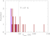 |
Fig. 3. Distribution of the minimum blackbody temperature Tmin required to explain the observed 1.2 mm brightness of z ∼ 6 QSOs. The Venemans et al. (2020) and SHELLQs samples are shown in brown and purple, respectively. Note that the 1.2 mm emission on approximately kiloparsec scales of a few bright objects can only be reproduced by hot dust with Td > 50 − 100 K. We used Td = 47 K, a standard reference value used in the literature (e.g., Venemans et al. 2020), to derive the dust masses of all QSOs with Tmin < 47 K. For hotter systems, we used Td = 1.2Tmin (see text for details). |
The dust masses derived for z ∼ 6 QSOs are shown in Fig. 1. They span a very wide mass range from ∼107 to ∼1010 M⊙, with bright QSOs having the larger dust contents. We applied the same method to compute dust masses for the other samples considered in this work, using the continuum flux densities as measured by ALMA and the source size derived from HST photometry (see Sect. 3.2), and compared the results with those published in the literature. We found an excellent agreement between our estimates obtained with Td = 47 K and those obtained with MAGPHYS for the ASPECS and COSMOS samples (see Fig. 1). For the ALPINE sample, the dust masses published by Pozzi et al. (2021) using a modified black body with Td = 25 K are a factor of 4 higher than those estimated here. This is mainly related to the cold dust temperature used in Pozzi et al. (2021): repeating the computation with Td = 25 K we obtained dust masses in excellent agreement with those of Pozzi et al. (2021). Figure 1 also shows the 3σ detection limit in dust mass for the ASPECS sample (rms ∼ 10 μJy), which is Md ∼ 2 × 10⁷ M⊙ at z = 1 and declines slowly toward higher redshifts. The typical detection limits of the other samples are from ∼2 (ALPINE, COSMOS, SHELLQs), to ∼10 (high-lum QSOs) times higher than the ASPECS limit.
We converted the dust masses into total gas masses by assuming δGDR = 200, as done by Aravena et al. (2020) for the ASPECS sample. Such a gas-to-dust mass ratio is in agreement with the expectations by chemical evolution models of evolved, massive disk galaxies with total baryonic mass Mtot > 1010 M⊙ (Calura et al. 2017), and with what is expected based on the metallicity of M* > 1010 M⊙ galaxies at z ∼ 6 in recent simulations (Torrey et al. 2019).
In addition, we derived the total gas mass of ALPINE galaxies and of z ∼ 6 QSO hosts by means of the [C II] line luminosity and the Zanella et al. (2018) calibration: Mgas/M⊙ = 31 × L[C II]/L⊙. The [C II]-based gas masses are generally consistent with those derived from the dust continuum (see left panel of Fig. 4).
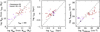 |
Fig. 4. Comparison between ISM mass (left), size (center) and column density (right) as derived from [C II] and dust continuum observations for the z ∼ 6 QSO samples. The ISM masses derived with the two methods agree for δGDR = 200. The [C II]-based sizes are on average ∼1.5 times larger than the dust continuum sizes. The total ISM column densities are on average higher for the dust continuum method, owing to the smaller sizes measured. Three sources with upper limits to their continuum size in the Venemans et al. (2020) sample are marked with arrows in the central and right panels. One SHELLQs source is not detected in the continuum, and is shown with an arrow in the left and right panels. For this and for another source in the same sample (both marked with large open squares in the central and right panels), the size could not be estimated, so we assumed it equal to the median of the sample. |
3.2. Galaxy size estimates
The relation between the galaxy size as measured through the stellar light, dust emission, or gas density profiles is subject of intense study. The effective radii found from HST photometry of distant galaxies (UV/optical rest-frame, i.e., probing the stellar light) are on average ∼1.5–1.7 times larger than those estimated with ALMA for the dust continuum emission (e.g., Fujimoto et al. 2017; Lang et al. 2019), whereas they are similar to those derived for the cold gas distribution, for example from CO data (Calistro Rivera et al. 2018). The reasons for this discrepancy could be ascribed to dust temperature and optical depth gradients, which may cause a steeper drop in the FIR/millimeter continuum emission at large radii (Calistro Rivera et al. 2018). If so, stellar emission would be a more reliable tracer of the spatial distribution of cold molecular gas, that is, of the bulk of the ISM, than the dust FIR-continuum emission. Recently, the effective radius of the [C II] line-emitting gas was measured by Fujimoto et al. (2020) for the ALPINE sample. For M* > 1010 M⊙ galaxies, the size of the [C II] emitting region was found to be on average ∼3 times larger than the HST UV/optical-rest size. [C II] emission traces both atomic and molecular gas, and atomic gas is known to be more diffuse (at least in local galaxies; Bigiel & Blitz 2012). Furthermore, large-scale, star-formation driven outflows of neutral gas are often observed in massive galaxies both in the local (Cazzoli et al. 2016; Roberts-Borsani et al. 2020) and distant (Ginolfi et al. 2020) Universe, which may also explain the larger [C II] sizes.
The resolution of the ALMA data available for both ASPECS and COSMOS z ∼ 3.3 galaxies (1.3 − 1.4″ FWHM) is not sharp enough to provide a reliable estimate of their cold gas extension. We then rely on UV/optical rest-frame measurements based on HST data. For ASPECS, we cross correlated the Aravena et al. (2020) sample with that presented by van der Wel et al. (2012), who run GALFIT (Peng et al. 2002, 2010) to measure the structural parameters of galaxies in the CANDELS fields selected by means of HST F160W photometry. The structural parameters relevant for this study are the effective radii re (actually, the half-light semimajor axes), Sersic indices n, and axial ratios q. The distributions of Sersic indices of the whole sample of van der Wel et al. (2012) and of the ASPECS subsample both peak at n = 1. We considered only the 32 ASPECS galaxies (23 from the main sample, and 9 from the secondary sample) where GALFIT returned a good fit (quality flag = 0). Typical sizes are re ∼ 3 − 4 kpc. For the COSMOS z ∼ 3.3 galaxies, we cross-correlated the Suzuki et al. (2021) sample with the COSMOS HST/ACS galaxy catalog (Leauthaud et al. 2007), which contains 1.2 millions galaxies detected in the F814W band down to 26.5 AB mag, and reports information about their half-light radii as measured from HST data. The UV sizes of galaxies in the Suzuki et al. (2021) sample are in the range re ∼ 1 − 2.5 kpc.
For the ALPINE sample (average ALMA beam size ∼0.9″), there are no public estimates of the size of the dust continuum emission, whereas [C II] sizes are available (Fujimoto et al. 2020) and will be used in the following. We also note that Fujimoto et al. (2020) derived optical/UV sizes for their targets using GALFIT on HST F814W and F160W photometric data. In particular, they were able to obtain a reliable size measurement (flag=0) for 7 massive ALPINE galaxies detected in the continuum (see Fig. 1 and Table 1).
For the sample of high-z QSO hosts, ALMA observations have been performed with a resolution of 0.3–0.5″, which is sufficient to resolve both dust and [C II] emission in most cases. The comparison between the [C II]-based and dust-based effective radii is shown in Fig. 4 (center). On average, the [C II]-based radii are ∼1.5 larger than dust-based radii. We recall that, in known high-z QSOs, the nuclear radiation largely outshines that of stars at optical/UV rest-wavelengths. As a result, in spite of the few attempts to separate the QSO light from that of its host through high-resolution HST observations (Mechtley et al. 2012; Marshall et al. 2020), no information is currently available about the stellar emission of z ∼ 6 QSO hosts.
4. ISM absorption estimates
4.1. ISM density profile and column toward galaxies’ nuclei
To estimate the ISM column density toward galaxy nuclei, we approximate galaxies as disks where both the light surface brightness and the gas density profiles decline exponentially along the radial direction. This is equivalent to assume a Sersic index of n = 1, which is consistent with the average light surface brightness profiles measured in the ASPECS and CANDELS samples. Furthermore, recent ALMA observations at 0.07″ resolution of a small sample of distant, submillimeter galaxies (Hodge et al. 2019) showed that their continuum emission is dominated by exponential dust disks, which also supports our assumptions. Given an exponential profile of the form:
where I0 is the central surface brightness and r0 is the scale (e-folding) radius, it is convenient to rewrite Eq. (6) in terms of the effective, or half-light radius re, defined as the radius enclosing half of the total luminosity:
Equation (6) then reads as:
For a pure exponential disk, re = 1.678 r0. We then consider a simple disk model for the gas distribution and work in cylindric coordinates. In the radial direction, we assume that the gas follows the same exponentially decreasing profile as the light surface brightness. For simplicity, we assume that there is no density gradient along the vertical (z) direction. A sketch of the adopted geometry is shown in Fig. 5. Denoting 2h as the disk thickness, the total gas surface density is:
 |
Fig. 5. Edge-on sketch of the adopted disk galaxy geometry. The darker shading reflects the higher ISM density of the assumed exponential profile. |
where ρ0 is the central gas volume density and Σgas, 0 = 2hρ0. By rewriting Eq. (9) in terms of the effective radius, one gets:
Observationally, from the total gas mass Mgas and effective radius re measured for a given galaxy, one can derive an average value for the gas surface density as:
This quantity can be easily related to the central gas surface density Σgas, 0 by considering that, by definition:
By combining Eqs. (9), (11), and (12), one derives:

Then, for a face-on view of a pure exponential disk galaxy one would measure a column density toward the nucleus equal to:

whereas for a random orientation angle θ between the galaxy axis and the line of sight, one has to integrate the density profile along the optical path ℓ (see the sketch in Fig. 5):
This gives:
![$$ \begin{aligned} N_{\mathrm{H},\ell } = \frac{r_0 \rho _0}{sin\theta } [ 1 - e^{-\frac{h}{r_0}tan\theta }] \; , \end{aligned} $$](/articles/aa/full_html/2022/10/aa43708-22/aa43708-22-eq23.gif)
which increases from hρ0 to r0ρ0 going from a face-on (θ = 0°) to an edge-on (θ = 90°) view. For random disk orientations, the average viewing angle is 1 radian, or ∼57.3o. By assuming a characteristic disk half scale-height h = 0.15re (Elmegreen & Elmegreen 2006; Bouché et al. 2015) and θ = 57.3o, from Eq. 16 one then finds a column density toward the nucleus equal to:

Therefore, for a purely exponential disk with random orientation, the average ISM column density toward the nucleus NH, ISM can be estimated as about twice the measured mean gas surface density Σgas.
We computed the column density toward the nucleus of ASPECS galaxies based on both Eqs. (16) and (17). In the thin-disk approximation, the orientation angle of each galaxy can be derived as θ = arcos(q), where q is the axial ratio reported by van der Wel et al. (2012) based on CANDELS F160W photometry. We note that the average axial ratio measured for ASPECS galaxies would correspond to θ ∼ 55°, remarkably similar to that expected for randomly oriented thin disks. The comparison between the column density obtained using a fixed, average orientation (Eq. (17)) versus those obtained from the individual orientations (Eq. (16)) is shown in Fig. 6. The two estimates generally agree within a factor of ∼2, and the Δlog NH, ISM distribution has mean around 0 and rms ∼ 0.15 dex. We therefore deem using a fixed, angle-average orientation a sufficiently good approximation for our purposes and utilize Eq. (17) to derive the ISM column densities in all the considered galaxy samples.
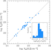 |
Fig. 6. Comparison between the ISM column densities toward the nucleus of ASPECS galaxies derived by assuming a fixed, average galaxy orientation (θ* = 57.3 deg) vs. those derived from individual galaxy orientations θ. The inset shows the distribution of the Δlog NH, ISM values: a Gaussian fit (dashed curve) is centered at about 0 (dotted line) and has rms ∼ 0.15 dex. |
In Fig. 4 (right) we show the comparison between the high-z QSO ISM column densities estimated using the [C II]-based ISM masses and sizes (NH,ISM,[C II]) versus those estimated with the dust-based gas masses and sizes (NH, ISM, dust). The column densities obtained with the two methods are in reasonable agreement with each other, but a nonlinear trend is visible, which is likely related to the overall system luminosity, as the high- and low-column regimes are mostly populated by high- (Venemans et al. 2020) and low- (SHELLQs) luminosity QSOs, respectively. Indeed, because of the well known [C II] luminosity deficit in FIR-bright systems (Malhotra et al. 2001; Graciá-Carpio et al. 2011; Díaz-Santos et al. 2017; Decarli et al. 2018), the ratio between the [C II]-based and the dust-based ISM masses decreases toward high QSO luminosities. More powerful QSOs have also stronger [C II] outflows (Bischetti et al. 2019) that may enhance the size difference between the [C II] and the dust emitting regions. Therefore, as the QSO luminosity increases, using the dust-based method one would derive larger ISM masses and smaller sizes than using the [C II]-based method, obtaining in turn the observed trend between the two column density estimates.
4.2. ISM clumpiness and obscured AGN fraction
In the previous sections we derived column density values assuming that the cold ISM is smoothly distributed across galaxy volumes. This is obviously not true: the molecular ISM phase, the one which is most concentrated and expected to produce most obscuration, is in fact distributed within dense clouds, which cover only a portion of the solid angle toward the nucleus. Here we aim to estimate the covering factor of these clouds and, in turn, the fraction of ISM-obscured AGN.
In the Milky Way, the average mass, radius, and surface density of molecular clouds are Mc = 105 M⊙, Rc = 30 pc, and Σc = 28 M⊙ pc−2, respectively (Miville-Deschênes et al. 2017). Their volume filling factor ϕ = ncVc, where nc is the number of clouds per unit volume, and Vc is the volume of each cloud, is about 1–2%. Such values may be radically different for massive galaxies at high redshift. As an example, the surface density of the individual molecular clouds detected in the “Snake” lensed galaxy at z = 1 (Dessauges-Zavadsky et al. 2019) is about 30 times higher than that of the Milky Way clouds. Furthermore, the cloud size and filling factor may be larger, hence producing significant coverage of the nucleus.
Similarly to what we did in the previous section for a smooth gas distribution, we assume that the cloud number density is exponentially decreasing along the galaxy radius and is constant in the vertical direction, that is:
where n0 is the number of clouds per unit volume at the galaxy center. Following Nenkova et al. (2008), the average number of clouds along a path ℓ at a given angle θ is given by:
where Nc = ncAc is the number of clouds per unit length and  is the cloud cross-sectional area. By integrating Eq. (19) we derive:
![$$ \begin{aligned} \mathcal{N} _{\rm T}(\theta ) = \frac{\tau }{\mathrm{sin}\theta } [ 1 - e^{-\epsilon \,\mathrm{tan}\theta }] \; , \end{aligned} $$](/articles/aa/full_html/2022/10/aa43708-22/aa43708-22-eq28.gif)
where τ = n0Acr0 and ϵ = h/r0 (see the analogous Eq. (16) for the total column density of a smooth medium).
Based on Eq. (20), the average number of clouds seen face-on or edge on is 𝒩T(0) = n0Ach and 𝒩T(π/2) = n0Acr0, respectively. So, the two parameters τ and ϵ in Eq. (20) correspond to the average number of clouds seen edge-on and to the ratio between the average number of clouds seen face-on versus edge-on, respectively. The variation of 𝒩T(θ) with θ is shown in Fig. 7 for a system with n0 = 270 kpc−3, Rc = (Ac/π)0.5 = 50 pc, ϵ = 0.25, re = 1.678r0 = 2.3 kpc. These numbers are representative of high-z galaxies. The assumed galaxy half-light radius re is, in fact, typical of massive systems at z = 2.5 (Allen et al. 2017). In addition, for Mc = 5 × 10⁶ M⊙ (which is a reasonable cloud mass at high-z, see the next sections), the total gas mass in the system is Mgas ∼ 1010 M⊙ (see, e.g., Eq. (23)), which is again typical of massive galaxies at z = 2.5 (Aravena et al. 2020). Clearly, the typical number of clouds intercepted along a given line of sight (e.g., Fig. 7) is subject to a series of uncertainties that increase when moving to progressively higher redshifts, where our knowledge of the average galaxy morphology (e.g., ϵ) and of the individual ISM cloud parameters (e.g., Rc) is poorer. Such uncertainties need to be kept in mind in the following analysis.
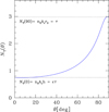 |
Fig. 7. Variation of the average number of ISM clouds along a given line of sight to the nucleus as a function of the viewing angle θ (90° is edge on) for a typical massive galaxy with Mgas ∼ 1010 M⊙ at z = 2.5. |
Once the average number of clouds along each line of sight is known, one can compute the total cloud covering factor to the nucleus, or, equivalently, the fraction of obscured nuclei fobsc in an unbiased sample of AGN (Nenkova et al. 2008):
We note that Eq. (21) assumes that individual clouds are optically thick. At soft X-ray energies, this condition is in fact satisfied given their typical column densities. As an example, the typical column density of molecular clouds in the Milky Way is NH ∼ 3 × 1021 cm−2 (Miville-Deschênes et al. 2017), meaning that they are optically thick to X-ray photons with E < 1 keV. The dependence of fobsc on the two parameters τ and ϵ is shown in Fig. 8.
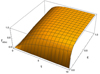 |
Fig. 8. Obscured AGN fraction as a function of τ, the average number of clouds along edge-on views, and ϵ, the ratio between the average number of clouds seen face-on vs. edge-on. |
The cloud number density at the galaxy center n0 can be related to the total number of clouds in the galaxy Ntot, and in turn to the total gas mass Mgas = NtotMc, as follows:
which gives:
By considering that  , re = 1.678r0, and Σc = Mc/Ac, Eq. (20) can be written as:
The main quantities that affect the average number of clouds observed in a given direction therefore depend only on the total galaxy gas surface density Σgas (which is an observable, see previous section), the gas surface density of each cloud Σc, and the galaxy “aspect ratio” ϵ. The meaning of Eq. (24) is clear: the number of clouds along a given direction increases as Σgas increases, as clouds are closer in space. Also, at a given Σgas, more clouds are intercepted along the line of sight if they are more diffuse, that is, if Σc decreases.
4.3. ISM clouds with a distribution of physical parameters
We now generalize the computations presented in Sect. 4.2 by moving from a single cloud type to a distribution of clouds with different radii Rc, masses Mc, and surface densities Σc. We assume that the shapes of these distributions are the same all over the galaxy volumes, and that only their normalizations, or the cloud number density, varies following the radial exponential decline described in the previous sections (see, e.g., Eq. (18)).
We first considered the distributions observed for molecular clouds in the Milky Way by Miville-Deschênes et al. (2017), who did not find any correlation between the cloud surface density and size. We then consider Σc and Rc as independent variables and write the number density of clouds at the galaxy center per unit cloud surface density and radius as:

where n(Rc) and n(Σc) are functions of only Rc and Σc, respectively, and k is a normalization constant.
By marginalizing over Σc and Rc one can write:

and

where no(Σc) and no(Rc) are the volume density of clouds at the galaxy center per unit Σc and Rc, respectively, I(Rc, *) = ∫n(Rc)dRc, and I(Σc, *) = ∫n(Σc)dΣc.
Miville-Deschênes et al. (2017) divide clouds in the Milky Way into inner clouds and outer clouds, depending on whether their distance to the Galactic center is smaller or larger than 8.5 kpc, respectively. The size distributions of inner and outer clouds both peak at Rc ∼ 30 pc and have similar shapes, whereas inner clouds are on average significantly denser and more massive, and contain ∼85% of the total gas mass in the Miville-Deschênes et al. (2017) catalog. We then derive the shape of no(Σc) and no(Rc), and hence of n(Rc) and n(Σc) by considering the Rc and Σc distributions of the inner Milky Way clouds, as these may be a better proxy of the clouds living in the compact environments of high-z galaxies. We downloaded the cloud catalog presented by Miville-Deschênes et al. (2017), and found that the Rc and Σc distributions can be well approximated by cut-off power-laws (Schechter functions) of the form:
and
with α = 1.7, Rc, * = 18 pc, β = 1.8, Σc, * = 25 M⊙ pc−2. With such approximations, I(Rc, *) and I(Σc, *) can be written as:
and
where  is the usual Gamma function. The total cloud number density at the galaxy center can then be written as:
Similarly, by recalling that the mass of each cloud is  , the total gas mass density at the galaxy center can be written as:

By integrating over the galaxy volume (see Eqs. (22), (23)), the total number of clouds and gas mass in a galaxy are then:
and
This simplified approach provides a satisfactory description of the overall cloud distribution and gas content of the Milky Way. As an example, for an input total gas mass equal to that contained in the inner Milky Way clouds (∼1.4 × 10⁹ M⊙, Miville-Deschênes et al. 2017), the model recovers the total number of clouds within a factor of ∼1.5 − 2. Furthermore, the model reproduces the inner Milky Way cloud distribution in the Rc versus Mc plane. The observed distribution is indeed well fit by the relation  and peaks at [Rc ∼ 35 pc, Mc ∼ 3 × 10⁵ M⊙], whereas in the model
  by definition, and the distribution peak is found at [Rc ∼ 30 pc, Mc ∼ 1.5 × 10⁵ M⊙].
4.4. ISM-obscured AGN fraction for different NH thresholds
The formalism developed in the previous sections allows us to compute the solid angle to galaxy nuclei intercepted by clouds above any given surface density threshold, or, equivalently, above any column density threshold NH, th. We can then compare our expectations with the fraction of AGN with NH > NH, th measured at different redshifts in wide and deep X-ray surveys. In addition, we can make forecasts about the obscured AGN populations at z > 5 − 6 which are still missing from our cosmic inventory.
For a cloud population with a distribution of sizes and surface densities, the number of clouds with NH > NH, th (Σc > Σth) per unit length can be written as:
where nc(Σc, Rc, r, z) = no(Σc, Rc)e−r/ro is the number density of clouds per unit cloud radius and surface density at a given position in the galaxy (r, z), and no(Σc, Rc) is the number density of clouds per unit cloud radius and surface density at the galaxy center, as defined in Eq. (25).
The average number of clouds with NH > NH, th along a path ℓ at a given angle θ is then given by (see Eq. (19)):
which leads to (see also Eq. (20)):
where

Here xth = Σth/Σc, * and  is the incomplete Gamma function. The normalization k of Eq. (39) can be expressed as a function of the total gas mass Mgas and galaxy scale ro by considering Eqs. (33) and (35). After some algebra one gets:
where 𝒢(β, xth) = Γ(β + 1, xth)/Γ(β + 1) decreases from 1 to 0 as xth increases from 0 to +∞. Equation (40) is the analog of Eq. (24), which was derived for a single cloud type. 𝒩T, th(θ) can be then estimated by specifying the total gas surface density and “aspect ratio” of the galaxy Σgas and ϵ, respectively, and assuming that the surface densities of individual molecular clouds are distributed as a Schechter function of slope β and characteristic density Σc, *.
Hence, for a population of identical galaxies, the fraction of ISM-obscured nuclei with NH > NH, th can be obtained as (see Eq. (21)):
In Eq. (41) one counts as obscured AGN with NH > NH, th only those systems where individual clouds with NH > NH, th fall along the line of sight. Of course, more than one cloud with NH < NH, th can lie along the line of sight and bring the total column density above the chosen threshold. Thus, the fractions of ISM-obscured AGN estimated from Eq. (41) should be considered as lower limits. We nonetheless note that for a population of high-z disk galaxies observed at an average orientation angle of θ = 57.3 (see Sect. 4.1), the average number of clouds along the line of sight is ∼1 (see, e.g., Fig. 7). We therefore consider Eq. (41) as a good proxy for the “true” fraction of ISM-obscured AGN with NH > NH, th.
5. Results
5.1. Evolution of the ISM column density
In Fig. 9 we show the distribution of the ISM column density as derived in Sect. 4.1 for the galaxy samples at different redshifts presented in Sect. 2. For ASPECS and COSMOS z ∼ 3.3 galaxies, we used the dust mass to estimate the total ISM mass and the UV/optical stellar size as a proxy for its size. For ALPINE and for the hosts of z ∼ 6 QSOs, we used [C II] data for both gas mass and size estimates. For comparison, for the 7 continuum-detected sources in ALPINE with a reliable HST size estimate (see Sect. 3.2) we also computed ISM column densities using the dust mass and the UV/optical stellar size as proxies for the total ISM mass and size, respectively. On average, as shown in Fig. 9, the column densities measured with this method are higher than those derived from [C II] data (the median value is higher by ∼0.5 dex). However, as discussed in Sect. 5.2, when accounting for selection biases, the ranges allowed for the column densities derived with the two methods fully overlap.
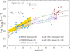 |
Fig. 9. ISM column density vs. redshift for different samples of M* > 1010 M⊙ galaxies as labeled. For ASPECS and COSMOS z ∼ 3.3 galaxies, ISM masses were derived from dust masses, and ISM sizes from UV/optical stellar sizes. For ALPINE galaxies and for z ∼ 6 QSO hosts both ISM masses and sizes were derived from [C II] data. For comparison, we also show for the ALPINE sample the results obtained using ISM masses derived from dust mass and ISM sizes derived from UV/optical stellar sizes (green open pentagons; see text for details). The upper bound of the light blue shaded area shows the median NH values obtained for the different samples (ASPECS was divided into two redshift bins). The lower bound shows the median NH values after including a conservative correction for incompleteness and observational biases (see Sect. 5.2). The NH ∝ (1 + z)4 solid curve is obtained by combining empirical trends for the gas mass and galaxy size and is normalized to NH = 1021 cm−2 at z = 0, which is consistent with the angle-averaged column density of the Milky Way (Willingale et al. 2013) and with the upper limit to the median column density of local massive galaxies as derived from the EDGE-CALIFA survey (Bolatto et al. 2017; big square at z = 0.1). The long-dashed curve running through the light-blue shaded area corresponds to (1 + z)3.3. The gold shaded area is from Buchner et al. (2017) as derived from the Illustris-1 simulation: lower and upper bounds are for galaxies with M* > 1010 M⊙ and M* > 1011 M⊙, respectively. The horizontal dashed line shows the column density corresponding to Compton-thick absorption. |
A steady increase of the ISM column density with redshfit is observed, with typical values going from ∼1022 cm−2 at z < 1 to ∼1024 cm−2 at z > 6. That is, the ISM in early, massive galaxies can reach values as high as Compton-thick and hence provide significant obscuration to any nuclear emission. Interestingly, at z ∼ 6, the ISM in the hosts of luminous QSOs (Venemans et al. 2020) is denser than what is measured in the hosts of less luminous QSOs (Izumi et al. 2018, 2019). Clearly, all known QSOs at z ∼ 6 are UV-bright and, by selection, are seen along lines of sight free from such heavy ISM columns.
By normalizing the ISM column density at z = 0 to the average value observed in the Milky Way, NH = 1021 cm−2 (Willingale et al. 2013), the increase of the average ISM column density with redshift can be parameterized as NH(z)/NH(0)∼(1 + z)4 (see black solid curve in Fig. 9). The adopted value for the z = 0 normalization is based on a single object and is then somewhat arbitrary. We nonetheless verified that this is consistent with what is measured in local samples of massive galaxies. To this end, we considered the 67 galaxies with M* > 1010 M⊙ in the extragalactic database for galaxy evolution drawn from the Calar Alto legacy integral field area survey (EDGE-CALIFA; Bolatto et al. 2017). Based on CO(1–0) observations with the combined array for millimeter-wave astronomy (CARMA; Bock et al. 2006), this survey measured the content and extent of the molecular gas reservoirs in a sample of nearby, z < 0.03 galaxies that were detected at 22 μm by the wide-field infrared survey explorer (WISE; Wright et al. 2010). We used those measurements to derive a median surface density of Σgas = 4.3 × 1021 cm−2, which translates (Eq. (17)) into a typical column density toward galaxy nuclei of NH = 9.0 × 1021 cm−2. Requiring a mid-IR detection with WISE preselects gas-rich galaxies. We then consider this column density estimate as an upper limit to the true, typical ISM obscuration in local massive galaxies, and we plot it as a downward arrow in Fig. 9.
Similarly, the overall ISM density versus redshift trend shown in Fig. 9 relies on samples of galaxies that are relatively bright in the FIR/millimeter domain, and one may then ask whether its validity is limited to those galaxy populations that are richer in gas at any redshift. We show in the next section that the ISM column density steeply increases with redshift even when accounting for selection biases, generalizing our results to the entire population of massive galaxies.
5.2. Median NH, ISM and correction of selection biases
By definition, any object with millimeter flux density below the ALMA detection limit is not included in the previous analysis. This can both bias high the overall NH, ISM measurements and distort its redshift evolution. Broadly speaking, as the fraction of massive, gas poor galaxies increases with decreasing redshift (Calura et al. 2008; Fontana et al. 2009), one may expect that the strongest bias is at low-z. The strength of this bias is however obviously also related to the sensitivity of the considered ALMA observations.
ASPECS is currently the deepest blind survey at 1.2 mm and is able to detect gas masses down to approximately 2.5 × 10⁹ M⊙ at any redshift above z ∼ 0.5. We then checked how many massive galaxies with M* > 1010 M⊙ in the part of the HUDF covered by ASPECS (∼2.1 × 2.1 arcmin2) went undetected by ALMA. We considered the catalog of stellar masses computed by Santini et al. (2015) in the whole GOODS-S area, which also includes the HUDF and probes stellar masses down to M* ∼ 3 × 10⁷ M⊙ up to z ∼ 3. Santini et al. (2015) compared several SED-based stellar mass estimates for GOODS-S galaxies as determined by different groups using the same photometry and redshift catalogs but different fitting codes, assumptions, priors, and parameter grids. In this work, we used the estimates flagged as “13aτ” in Santini et al. (2015; see their Table 1), which were derived assuming a Chabrier IMF and an exponentially decreasing star formation history, as they provide the best agreement with those published by Aravena et al. (2020) (we derived a null offset and ∼0.25 dex rms for the mass ratio distribution of common objects). We matched the Santini et al. (2015) catalog with that of van der Wel et al. (2012) and found 23 galaxies in the ASPECS survey area with reliable structural parameters (q = 0 in van der Wel et al. 2012), redshift in the range z = 0.5 − 3 and stellar mass M* > 1010 M⊙ (i.e., using the same cuts applied to the Aravena et al. 2020 sample). Their size distribution is similar to that of ASPECS galaxies. We then used the size measured by van der Wel et al. (2012) and assumed a gas mass of 2.5 × 10⁹ M⊙ to derive upper limits to their ISM column densities. Many of these limits fall in the cloud occupied by ASPECS galaxies in Fig. 9. However, in order to have a conservative estimate of the lowest possible median column density of the entire population of massive galaxies at z = 0.5 − 3 (i.e., both detected and undetected by ALMA), we considered all of these 23 objects to lie below the lower envelope of the NH versus z distribution of ASPECS galaxies. By dividing the sample into two redshift bins, we found that, when ALMA undetected galaxies are included, the median NH, ISM value decreases from 4 × 1022 cm−2 to 7 × 1021 cm−2 at z = 1, and from 6 × 1022 cm−2 to 3 × 1022 cm−2 at z = 2 (see Fig. 9). The quoted NH ranges can therefore be considered as bracketing the true median values in both redshift bins.
The six COSMOS z ∼ 3.3 galaxies detected at 1.2 mm are drawn from the sample of Suzuki et al. (2021), who observed with ALMA twelve star-forming galaxies (11 with M* > 1010 M⊙) with reliable gas phase metallicity measurements based on near-IR spectroscopy. Incidentally, by means of the dust-to-gas mass ratio δGDR versus gas-phase metallicity relation derived by Magdis et al. (2012), Suzuki et al. (2021) estimated an average δGDR = 210 for their sample, in excellent agreement with what is assumed throughout this work (δGDR = 200). The median column density of the six ALMA-detected galaxies is log NH, ISM ∼ 23.6. Assuming that the five ALMA-undetected massive galaxies in Suzuki et al. (2021) have gas masses and column densities smaller than ALMA-detected galaxies, the median ISM column density of the whole sample in Suzuki et al. (2021) would then coincide with the lowest column density measured, log NH, ISM ∼ 22.9 (see Fig. 9). All star-forming galaxies in Suzuki et al. (2021) lie on the main sequence. Since quiescent, gas-poor systems represent only a few percent of the whole population of massive galaxies at z > 3 (Girelli et al. 2019), we consider the median NH, ISM estimated above as representative of the whole population.
Out of the 27 galaxies with M* > 1010 M⊙ in the ALPINE sample of Fujimoto et al. (2020), 21 were detected in [C II]. The median column density of the nine galaxies with a reliable [C II]-based size estimate is log NH, ISM = 23.5 (see Fig. 9, we plot it at z = 5). We verified that the 12 galaxies with no good [C II]-size estimate have an NH, ISM distribution similar to that shown in Fig. 9, and we have assumed that the six [C II]-undetected galaxies all have NH, ISM below the lowest measured value for the detected galaxies. This brings the corrected median log NH, ISM value of the whole sample to 23.2. Similarly to the COSMOS z ∼ 3.3 sample, ALPINE galaxies lie on the main sequence (Fujimoto et al. 2020), and therefore we consider the corrected median NH, ISM as representative of the whole population of massive galaxies at z ∼ 5. We repeated the same exercise on the ALPINE sample by considering the ISM column densities derived from dust mass and UV/optical sizes. The median column density of the 7 continuum detected galaxies with reliable HST size is log NH, ISM ∼ 24. When considering the whole sample of 13 dust-detected galaxies without requirements on the size reliability, we found that the lowest column density of the sample is about log NH, ISM = 22.8. By conservatively assuming that the 14 continuum undetected galaxies all have column densities below this value, we estimate that a plausible range for the median dust-based NH, ISM is 22.8–24, which is larger than the range derived from [C II] data and fully encompasses it (see also Fig. 9).
For the sample of z ∼ 6 QSO hosts, we note that any correction to account for ALMA undetected objects does not affect significantly the mean NH, ISM derived from ALMA detections only. As a matter of fact, all of the seven low-luminosity QSOs observed by Izumi et al. (2018, 2019) are detected in [C II], and six of them also in the continuum. The sample of high-luminosity QSOs in Venemans et al. (2020) instead includes only objects that were previously known to be FIR-bright. We evaluate the non-detection rate of high-luminosity QSOs hosts based on the sample discussed in Venemans et al. (2018) and Decarli et al. (2018), which largely overlap with the Venemans et al. (2020) sample and include targets selected by UV luminosity only. The non-detection rate in that sample is less than 15% for both [C II] and continuum observations. As the ALMA observations in Venemans et al. (2020) are on average more sensitive than in Venemans et al. (2018), this non-detection rate can be considered as an upper limit. Nonetheless, we checked that assuming a 15% non-detection rate for luminous high-z QSOs would change the median NH, ISM estimates, either based on [C II] or continuum emission, by less than 10%, and therefore we neglected this correction. To derive a representative median NH, ISM for the entire population of z ∼ 6 QSO hosts, one has instead to consider that the number of ALMA observations of low-luminosity and high-luminosity QSOs do not reflect the actual abundance of the two populations. Bright QSOs were indeed discovered earlier and are easier targets, and then dominate the statistics of currently observed objects. As shown in Fig. 4, luminous QSOs are also the ones with larger gas masses and column densities, and therefore their median NH, ISM cannot be considered as representative of the whole population. To correct for this, we considered the UV-rest luminosity function (LF) of z ∼ 6 QSOs published by Matsuoka et al. (2019), which combines the results from SHELLQs with those of shallower, wider-area optical surveys. By first integrating the QSO LF in the range MUV = [ − 22, −25] covered by the Izumi et al. (2018, 2019) samples, and then at magnitudes MUV < −25, as typical of the Venemans et al. (2020) sample, we estimate that low-luminosity QSOs are about 9 times more abundant than high-luminosity QSOs. We then smoothed the observed NH, ISM distributions of high- and low-luminosity QSOs with a boxcar of 1 dex in log NH, ISM, and resampled each distribution 1000 and 9000 times, respectively. The corrected median value of the final distribution is log NH, ISM = 23.7, which we consider as representative of the observed population of z > 6 QSOs, that is, of z ∼ 6 massive galaxies. When compared with the allowed ranges for the median column density of massive galaxies at lower redshifts (see Fig. 9), this calls for an increase of the median ISM column density with redshift as (1 + z)δ, where δ is in the range 2.3–3.6. When the median column density of local galaxies is fixed to NH = 1021cm−2, as observed in the Milky Way (Willingale et al. 2013), the cosmic evolution of the corrected median ISM column density is best described by δ = 3.3 (see Fig. 9).
5.3. Comparison with the median AGN X-ray column density
In Fig. 10 we compare the evolution of the median ISM column density derived in the previous section, both as measured and corrected for selection biases, with the median column densities derived from X-ray observations of large AGN samples. To minimize the biases against heavily obscured AGN we considered either results from the deep Chandra and XMM-Newton observations of the CDFS (Iwasawa et al. 2012, 2020; Liu et al. 2017; Vito et al. 2018), or, for the local Universe, results from AGN samples selected at energies above ∼10 keV with Swift/BAT (Burlon et al. 2011) or NuSTAR (Zappacosta et al. 2018).
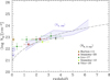 |
Fig. 10. Comparison between the evolution of the median column density of the ISM (light blue shaded area and black dashed curve – same meaning as in Fig. 9) and of the median absorption column density measured in different AGN samples through X-ray spectroscopy (see text for details). At z ≳ 1.5 − 2 the ISM column density becomes comparable to that measured in the X-rays. |
As shown in Fig. 10, the median column densities derived for the X-ray nuclear obscuration are on the same order of the ISM column densities, especially at z ≳ 1.5 − 2. This indicates that the ISM may in fact produce a substantial fraction of the nuclear obscuration measured around distant SMBHs. Instead, in the local Universe, and likely up to z ∼ 1.5 − 2, the median X-ray derived column densities appear in excess of what can be produced by the ISM, suggesting that most of the nuclear obscuration is produced on small scales by the AGN torus.
We note that several caveats apply to the above comparison: first, the considered AGN samples generally do not contain any cut in host stellar mass, whereas our ISM density computations are valid for systems with M* > 1010 M⊙. Most AGN in the considered X-ray samples, however, are likely hosted by massive galaxies. For example, we checked that this is in fact the case for the BAT and for the Vito et al. (2018) samples, and that the average column densities obtained cutting at M* > 1010 M⊙ are in good agreement with those of the total samples. Second, detecting the most heavily obscured, Compton-thick AGN is hard even for the deepest X-ray surveys (Lambrides et al. 2020). As a result, completeness corrections are difficult, and the median column density estimates may have been underestimated. Third, the fraction of obscured AGN is known to decrease with X-ray luminosity (Gilli et al. 2007; Hasinger 2008), which again may bias low the derived median NH estimates, especially toward high redshifts where low-luminosity systems cannot be detected effectively. We defer to the Discussion a more detailed comparison between the X-ray and ISM obscuration. Here it is just worth remarking that, at high-z, the ISM column densities are on the same order of what is measured via X-ray absorption.
5.4. Redshift evolution of the ISM-obscured AGN fraction
The formalism developed in Sects. 4.2–4.4, can be used to follow the redshift evolution of the average number of ISM clouds toward galaxy nuclei and, in turn, of the ISM-obscured AGN fraction. Since the surface density of individual molecular clouds has been found to significantly increase with redshift for a given cloud size (Dessauges-Zavadsky et al. 2019), we allow the characteristic surface density Σc, * of molecular clouds to increase with redshift as Σc, *(z) = Σc, *(0)(1 + z)γ, exploring the range γ = 2 − 3 to account for the large uncertainties associated with the above trend. We instead assume for simplicity that the distribution of the cloud radii does not vary with redshift, as observations of molecular clouds in distant galaxies are unavoidably biased against small systems and hence cannot probe the entire size distribution. As an example, the ALMA observations of the Snake lensed galaxy at z = 1 in Dessauges-Zavadsky et al. (2019) could only resolve clouds with Rc > 30 pc.
The redshift evolution of the ISM-obscured AGN fraction above a given NH, ISM threshold is derived using Eqs. (40) and (41). The redshift dependence is encapsulated in the function (Σgas/Σc, *)×𝒢(β, xth)∝(1 + z)δ − γ𝒢(β, xth(z, γ)). Once the characteristic gas surface density and cloud surface density distribution of galaxies at z = 0 are specified (that is, Σgas(0), Σc, *(0), and β), and assuming that the ratio, ϵ, between the number of galaxy clouds seen face-on versus edge-on is the same at all redshifts, the cosmic evolution of the ISM-obscured AGN fraction is determined by how fast the galaxy total gas surface density increases with respect to the characteristic cloud surface density (1 + z)δ − γ modulated by 𝒢(β, xth(z, γ)). 𝒢 depends on z and γ through the lower integration limit xth = Σth/(Σc, *(1 + z)γ): for a fixed NH (Σ) threshold, it increases with increasing redshift at a rate that grows with increasing γ.
We show in Fig. 11 the cosmic evolution of the fraction of ISM-obscured AGN for γ = 2 and 3, and for three different column density thresholds, Nth = 1022, 1023, and 1024 cm−2. Based on the evolution of the ISM column density (Sect. 5.2), which is linked to the total gas surface density through Eq. (17), we assume δ = 3.3 to describe the increase in the total gas surface density with redshift. We also fixed the total gas surface density of local galaxies to Σobs(0)∼5 × 1020 cm−2, corresponding to an average column density toward the nucleus of NH ∼ 1021 cm−2, and the shape parameters of the cloud density distribution to what is observed for the inner Milky Way clouds (Σc, *(0) = 25 M⊙ pc−2, β = 1.8). We also fixed ϵ = 0.25, consistently with the adopted value of h/re = 0.15 assumed in Sect. 4.1.
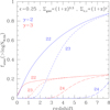 |
Fig. 11. Expected redshift evolution of the ISM-obscured AGN fraction. Blue curves consider a slower (γ = 2) increase with redshift of the characteristic cloud density Σc, *. Red curves assume a faster increase (γ = 3). Labels refer to different thresholds in log column density (see text for details). |
As shown in Fig. 11, given the global increase of the ISM column density with redshift, the cosmic evolution of the ISM-obscured AGN fraction heavily depends on the evolution of the characteristic cloud density Σc, *: on the one hand, if Σc, * rapidly grows with redshift (γ = 3), the fraction of ISM-obscured AGN evolves weakly, as only a few, dense clouds are needed to match the total column density increase with redshift. On the other hand, if Σc, * grows slowly (γ = 2), more clouds are needed to produce the same column, and hence there are more chances to see the nucleus through a cloud. In both cases, at z = 0, the fraction of ISM-obscured AGN is expected to be below 5% for a column density threshold of NH, th = 1022 cm−2, and to be negligible for NH, th = 1023 cm−2 (see Fig. 11). At z = 3.5, instead, fobsc(> 1023) grows from 0.21 to 0.43 when moving from γ = 3 to γ = 2. As expected, the fraction of heavily obscured nuclei fobsc(> 1023) is always smaller than what is obtained by relaxing the absorption threshold fobsc(> 1022), but the two numbers progressively get closer toward higher redshifts as the fraction of low-column clouds in galaxies gets smaller. Remarkably, in the γ = 2 scenario, more than 80% of all early SMBHs at z > 6 may be obscured by the ISM in their hosts. At even higher redshifts, z > 8, one may further expect to see Compton-thick absorption from the ISM in about 15–20% of accreting SMBHs. Clearly, the cosmic evolution of the surface density of individual molecular clouds is largely unknown. On the one hand, by comparing the typical densities of clouds in the Snake galaxy at z ∼ 1 (Dessauges-Zavadsky et al. 2019) with that of Milky Way clouds one would get γ > 3 (which may be however biased high as selection effects would favor the detection of bigger and denser clouds in the Snake). On the other hand, theory works on z ∼ 6 galaxies (e.g., Vallini et al. 2018, 2019) often assume fiducial cloud sizes and masses corresponding to surface densities similar to what is measured in the Milky Way and other nearby star-forming galaxies, meaning γ = 0. We actually do not consider the γ = 2 scenario as the more plausible a priori, but anticipate that it provides the best representation of the obscured AGN fractions measured at different cosmic times (see Sect. 6.3).
6. Discussion
6.1. ISM column density: uncertainties and empirical trends
In Sect. 5.2, we showed that the median column density of massive galaxies increases with redshift as NH ∝ (1 + z)δ, where δ = 3.3. The exact value of the slope δ is admittedly uncertain, and an adequate representation of the median column density values observed at different redshifts would still be obtained for δ = 2.3 − 3.6. Nonetheless, the derived slope is similar to what one would derive from simple empirical trends reported in the literature about the cosmic evolution of the average gas mass and size of massive galaxies. The gas mass of galaxies is in fact known to rapidly increase with redshift as (1 + z)a, with a ∼ 2 (Scoville et al. 2017; Tacconi et al. 2018; Liu et al. 2019). For instance, for main sequence star-forming galaxies, Scoville et al. (2017) found that the ISM content increases as a function of redshift as MISM ∝ (1 + z)1.84 ± 0.14, and is also a weak function of stellar mass ( , see their Eq. (6)). We note that the Scoville et al. (2017) sample is essentially made by galaxies with stellar masses in the same range of the previously considered ASPECS sample, M* = 1 − 30 × 1010 M⊙ (see Sect. 2.1): in fact, fewer than 3% of the > 700 objects in Scoville et al. (2017) have masses below 1010 M⊙ and 1% have masses above 3 × 10¹¹ M⊙. The size of galaxies is known to decrease with redshift (e.g., Allen et al. 2017). This decrease is commonly parameterized as re ∝ (1 + z)−b, where re is the effective (or half-light) radius of the galaxy and b ∼ 1.0. The exact value of b depends on the specifics of the galaxy population under consideration. For instance, Shibuya et al. (2016, 2019) measured b = 1.20 and 1.37 for LBGs and LAEs, respectively. For a mass-complete sample of star-forming galaxies with M* > 1010 M⊙ in the redshift range z = 1 − 7 selected in the CANDELS fields, Allen et al. (2017) found b in the range 0.9–1.0, depending on the adopted IMF and analysis methodology. They measured the effective radius by means of HST F160W photometry. The upper mass bound of the Allen et al. (2017) sample is again M* ∼ 3 × 10¹¹ M⊙. Assuming that gas and stars follow the same spatial distribution and then have equal effective radii, by combining the empirical relations found by Scoville et al. (2017) and Allen et al. (2017) one would trivially get that the average ISM volume and surface density increase with redshift as (1 + z)5 and (1 + z)4, respectively, for galaxies within the same stellar mass range considered in this work. The slope of the column density relation, δ = 4, derived from this simple exercise is then similar to what we derive in Sect. 5.2 from our samples (δ = 3.3), and again points to a steep increase of the ISM density toward early epochs.
Concerns in the evolution rates derived for the ISM density may be related to how gas masses and sizes have been estimated. As discussed in Sect. 3.2, the effective radii of stellar emission as probed by UV/optical rest-frame data are similar to those derived from CO emission, but a factor of 1.5–1.7 larger than those measured from dust continuum emission (Fujimoto et al. 2017; Lang et al. 2019). Calistro Rivera et al. (2018) suggest that this difference is due to temperature and optical depth gradients which cause a steeper drop in the FIR emission at large radii: stellar emission would then be a more reliable tracer of the spatial distribution of cold molecular gas, as also found by recent numerical simulations (Popping et al. 2022). This seems to be true at all redshifts, as the effective radius measured from ALMA continuum emission decreases with redshift with the same rate (b ∼ 1) as measured from CANDELS (UV/optical-rest) photometry (Fujimoto et al. 2017). In Sect. 3.2 we used for ASPECS and COSMOS z ∼ 3.3 galaxies the stellar sizes derived from HST photometry. For the z > 4 samples, ALPINE and z ∼ 6 QSOs, [C II]-based size measurements are available and we resorted to those. For the ALPINE sample, the [C II]-based sizes are ∼2× larger than the rest-frame UV-continuum size measured with HST (Fujimoto et al. 2020) We note that, as yet, no public information is available on the dust-continuum sizes for this sample. For the high-z QSOs samples, [C II]-based sizes are on average ∼1.5× larger than those estimated from the dust continuum (the host UV/optical stellar emission is as yet undetected in these systems). Hence, in general, we may conclude that: (i) using dust-based measurements would likely produce a global increase of the ISM densities by a factor of ∼2 − 4 at all redshifts, making ISM-obscuration of AGN even stronger; (ii) replacing the [C II] sizes with the optical/UV-rest sizes (when available) would increase by a factor of ∼4 the ISM densities of our highest redshifts samples, hence making the observed evolution even steeper.
6.2. Adding the parsec-scale torus
In Sect. 5.4 we discussed how the redshift evolution of the ISM-obscured AGN fraction depends on our cloud model assumptions, particularly on the evolution of the cloud characteristic density Σc, *. Figure 11 shows that, if the evolution in Σc, * is not too fast, the fraction of ISM-obscured AGN rapidly increases toward early cosmic epochs. The model predictions, however, cannot be directly compared with the observed fractions of X-ray obscured AGN, as these include any absorption along the line of sight, especially that produced by dense, dusty gas around the nucleus. This so-called torus, is thought to be azimuthally distributed within a few to tens of parsecs from the SMBH (e.g., Combes et al. 2019; García-Burillo et al. 2019). Locally, the torus covering factor is used to explain the abundance of heavily obscured SMBHs with NH > 1023 cm−2 (Risaliti et al. 1999; Marchesi et al. 2018), as opposed to the local global ISM, which, at z ∼ 0, can only produce mild obscuration (NH, ISM ≲ 1022 cm−2 ; see Sect. 5.1 and Fig. 9).
Recent progress has been made in both observations (Zhao et al. 2021; Torres-Albà et al. 2021) and modeling (Baloković et al. 2018; Buchner et al. 2019) of the torus component. Accurate fits to the NuSTAR and XMM-Netwon spectra of local Seyfert 2 galaxies (Marchesi et al. 2019; Zhao et al. 2021) revealed that the torus covering factor is about 0.6–0.7. Although the torus structure is likely complex and patchy, in the simple assumption of a medium uniformly distributed in a donut-like shape around the SMBH, a covering factor of 0.71 corresponds to a half-opening angle of θtorus = 45°. Moving from Seyfert to QSO luminosities, the torus covering factor is known to decrease, possibly because of the increased radiation pressure (Maiolino et al. 2007; Lusso et al. 2013; Ricci et al. 2017): at Lbol ∼ 1046 − 47 L⊙, the torus covering factor is estimated to be 0.4–0.5, where 0.5 corresponds to a half-opening angle of 60°. Here we shall now assume that the torus covering factor does not evolve with redshift. This is supported by the lack of evolution in the broadband SEDs of luminous quasars, which are remarkably self-similar up to the highest redshifts, z ∼ 6 − 7 (Barnett et al. 2015; Nanni et al. 2018). In particular, no evolution has been observed in the typical ratio ℛ between the QSO UV/optical and mid-IR luminosity (Leipski et al. 2014; Bianchini et al. 2019), which is considered as a proxy for the fraction of nuclear radiation reprocessed by hot dust (T < 1500 K) within a few parsecs of the nucleus, that is, for the torus covering factor. For example, Bianchini et al. (2019) divided a sample of > 250 000 luminous QSOs at 1 < z < 5 into three redshift bins populated by objects with similar luminosities1 and found a remarkably constant average value ℛ ∼ 1.1 in the three bins. This suggests that the covering factor of the small-scale, circumnuclear medium is primarily regulated by QSO feedback across cosmic times.
ALMA observations of nearby Seyfert galaxies at parsec-scale resolution showed that the torus axis and the galaxy disk axis are often misaligned (Combes et al. 2019). Accounting for any torus-disk misalignment in our model (see below) would increase the total gas covering factor around the nucleus, and, in turn, the total obscured fraction of AGN at any redshift. For simplicity, we considered the torus and the galaxy disk as coaxial (see Fig. 12), keeping in mind that the derived obscured AGN fractions may represent lower limits. Again, for the sake of simplicity, we assumed that the torus produces Compton-thick absorption through all lines of sight crossing it. We considered two cases for its half-opening angle: θtorus = 45° or 60°. In this simple configuration, the total fraction of obscured AGN can be simply obtained with Eq. (41) by using θtorus instead of 90° as the integral upper bound, as all lines of sight with θtorus < θ < 90° are now heavily obscured by the torus component.
 |
Fig. 12. Edge-on view of the considered geometry for the ISM clouds and the torus (not to scale). |
6.3. Cosmic evolution of the total nuclear obscuration
In Fig. 13 we show the effects of adding the small-scale torus absorption to the large-scale ISM absorption for different assumptions on the evolution of the characteristic cloud surface density. As in Fig. 11, we fixed the evolution rate of the average ISM density to δ = 3.3 and the ratio between the average number of ISM clouds crossed face-on versus edge-on to ϵ = 0.25. If the evolution in Σc, * is fast, γ = 3, the torus covering factor overwhelms that of ISM clouds. In this case, the obscured AGN fraction is expected to mildly increase up to z ≈ 1 − 2 and then stay almost constant. For γ = 2 instead, the rapid increase in the ISM covering factor with redshift is not washed out by the constant torus coverage, and an overall increase of the obscured AGN fraction toward early cosmic times is then expected. In Fig. 14 we compare the model curves for γ = 2 with the obscured AGN fractions measured in different X-ray samples for two different NH thresholds (1022 and 1023 cm−2). In addition to the X-ray samples already used in Sect. 5.3, we also considered the results from published AGN X-ray luminosity functions that try to correct for selection biases against heavily obscured sources (Ueda et al. 2014; Aird et al. 2015; Buchner et al. 2015). As the fraction of obscured AGN depends on X-ray luminosity (Gilli et al. 2007; Hasinger 2008; see also the discussion above), we considered separately high-luminosity and low-luminosity AGN, using samples with intrinsic, median 2-10 keV luminosity log LX = 44 ± 0.3 erg s−1 for the high-luminosity bin, or log LX < 43 erg s−1 for the low-luminosity bin.
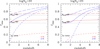 |
Fig. 13. Total fraction of obscured AGN with log NH > 22 (left panel) and log NH > 23 (right panel) vs. redshift for different combinations of large-scale (ISM) and small-scale (torus) obscuration. All curves are for δ = 3.3 and ϵ = 0.25. The characteristic surface density Σc, * of ISM clouds is assumed to evolve as ∝(1 + z)γ, with γ = 2 (blue curves) or γ = 3 (red curves). Short dashed lines refer to ISM-only obscuration (i.e., no torus considered, as in Fig. 11). Long dashed and solid lines show the total obscured AGN fraction when adding a torus with half-opening angle θtorus = 45° and 60°, respectively. The horizontal dotted lines show the obscured AGN fraction expected by torus-only obscuration. |
The ISM model with γ = 2, combined with a torus with θtorus = 60° (the expected opening angle at log LX ∼ 44; see above), is able to explain quantitatively the increase with cosmic time in the fractions of luminous AGN with NH > 1022 cm−2 and NH > 1023 cm−2 (see solid lines in Fig. 14). In Fig. 15 we show the same comparison for obscured AGN of lower luminosities (log LX ∼ 42.5 erg s−1). Here we also considered a recent update on the fraction of obscured AGN measured locally that is based on the BAT 100-month sample (Marchesi et al., in prep.). At these low luminosities, measurements of the obscured AGN fraction are clearly sparser and incomplete, especially toward high redshifts, but the same model of ISM plus torus absorption (this time using a torus opening angle θtorus = 45°, as expected for low-luminosity AGN) provides a good match to the data.
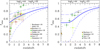 |
Fig. 14. Total fraction of obscured AGN with log NH > 22 (left panel) and log NH > 23 (right panel) vs. redshift measured in different X-ray samples (see labels) and compared with model curves of large-scale (ISM) plus small-scale (torus) obscuration. Only samples with median log LX ≈ 44 have been considered here (see text for details). Curves have the same meaning as in Fig. 13. The model with γ = 2 and θtorus = 60° (thick solid blue line) provides a good representation of the data. |
Our results are subject to a number of uncertainties, both in the data and in the model, as discussed below. In Sect. 5.3, we mentioned that no preselection in their host stellar mass was originally applied to the X-ray AGN samples considered here. Nonetheless, we expect that the obscured AGN fractions would not change significantly when cutting the sample at M* > 1010 M⊙, as most AGN in those samples are likely hosted by massive galaxies. Also, because of the difficulties to detect Compton-thick AGN in sizable numbers, many studies just measure the fraction of obscured objects within the Compton-thin AGN population (log NH < 24). Assuming that the relative abundance of Compton-thick AGN is similar to what is assumed in the population synthesis model of the cosmic X-ray background of Gilli et al. (2007), we estimate that a plausible correction for the missing Compton-thick AGN would increase the total fractions of obscured AGN by Δfobsc ∼ 0.1 on average. Finally, although the observed increase in the obscured AGN fraction may look somewhat steeper than the expectations (Fig. 14), we note that the model curves are not meant to best-fit the data and may be adjusted by varying the input parameters. For instance, one could modify the face-on versus edge-on cloud number ratio ϵ, or introduce different density gradients in the cloud distribution along the galaxy disk thickness, to cope with the variations in the galaxy morphology across cosmic time, as the fraction of mergers and irregular systems is known to increase with redshift (Mortlock et al. 2013; Whitney et al. 2021). In addition, one cannot entirely rule out a redshift evolution of the torus covering factor, although this might be at odds with the lack of evolution in the UV/optical to mid-IR luminosity ratio observed in luminous QSOs at different redshifts (Bianchini et al. 2019) and discussed in Sect. 6.2. For example, the observed increase in the obscured AGN fractions shown in Fig. 14 could be also reproduced assuming that the fraction of ISM-obscured AGN does not evolve significantly (i.e., γ = 3), but that the torus half-opening angle evolves from θtorus = 60° at z = 0 to θtorus = 45° at z ∼ 4 (see, e.g., Fig. 13). Exploring the full model parameter space is, however, beyond the scope of this paper and is deferred to future work. With all this in mind, we believe that our combined, ISM plus torus model provides a good description of the observed trends: obscuration by the ISM alone would be too small to explain local data; torus obscuration only would not explain the observed increase toward early cosmic times.
Interestingly, such a model predicts that the fraction of obscured AGN is about 80–85% at z = 6 and > 90% at z > 8 (∼50–55% of the systems being Compton-thick). That is, the bulk of SMBHs in the first 0.5–1 Gyr of the Universe are expected to be hidden by dust and gas distributed across all galaxy scales, from pc to kpc. Currently, we do not have any known example of such obscured systems. The best candidates to date may hide among the population of z ∼ 6 LBGs and QSOs discovered by the Subaru HSC surveys. Among the published 93 SHELLQs QSOs, 18 objects in fact exhibit narrow Lyα with FWHM < 500 km s−1. Since the Lyα luminosity exceeds 1043 erg s−1, as in AGN-dominated systems (Sobral et al. 2018), they are tentatively classified as QSOs. The origin of these narrow line (NL) objects is, however, not entirely clear, since star-forming galaxies could produce strong Lyα and high-ionization condition reminiscent to AGN (Nakajima et al. 2018a). Deep X-ray observations will be a viable method to reveal whether obscured QSOs really hide among them.
6.4. Comparison with other works
Buchner et al. (2017) used X-ray spectra of long gamma-ray burst (GRB) afterglows to derive ISM column densities in a sample of galaxies in the redshift range 0.5–3 with > 90% redshift completeness and selected independently of their stellar mass (SHOALS sample; Perley et al. 2016). They found a positive correlation between ISM column density and galaxy stellar mass of the form  . The median column density of their high-mass sample with M* > 1010 M⊙, is log NH, ISM = 22.13 ± 0.10. This value was derived using GRB at random locations along galaxy disks, and would increase to log NH, ISM ∼ 22.4 (Eq. (17)) when seen from galaxy nuclei. This is already in agreement within a factor of ∼2 with the median ISM column density toward the nuclei of ASPECS galaxies, cut at the same mass threshold, and with a similar redshift range (log NH, ISM = 22.70 ± 0.10), but the agreement may further improve by considering that: (i) as reported in Perley et al. (2016), the GRB rate per unit star formation in the SHOALS sample is constant in galaxies with gas-phase metallicity below the solar value but heavily suppressed in more metal-rich environments. Therefore, the most massive and gas-rich galaxies may be under-represented in GRB-selected samples; (ii) as discussed in Sect. 5.2, the ASPECS sample only includes gas-rich galaxies detected by ALMA with Mgas ≳ 3 × 10⁹ M⊙ and, when accounting for ALMA-undetected galaxies, the true average column density of massive galaxies at z = 0.5 − 3 would likely decrease by a factor of ≈2. In summary, our ISM column density estimates are in good agreement with those of Buchner et al. (2017) for galaxies with similar stellar masses and redshifts. However, as opposed to Buchner et al. (2017), we found evidence that NH, ISM evolves with redshift even within the ASPECS sample, with typical values increasing by more than one dex from z = 0.5 to z = 3 (see, e.g., Fig. 9).
Recently, Masoura et al. (2021) analyzed the host galaxy properties of > 300 X-ray selected AGN in the XMM-XXL survey (Pierre et al. 2016), without finding any strong correlation between AGN type (obscured vs. unobscured) and host physical properties. In particular, they found no correlation between the nuclear column density as estimated from X-ray colors (hardness ratios, HR) and star formation rate, and hence suggested that the obscuration is not related to the large-scale star formation in the galaxy, that is, to the host ISM. We note that our findings are not in contrast with those of Masoura et al. (2021). In fact, in our model both obscured and unobscured AGN share the same ISM content, and hence the same SFR, and the AGN type classification depends only on the chance that the line of sight to the nucleus is occulted by an ISM cloud. It is then the fraction of obscured AGN, rather than the AGN average column density, the quantity we expect to correlate more with SFR in a given population of galaxies.
6.5. Comparison with theory
In Fig. 9 we compared the redshift evolution measured for the ISM density with the expectations extracted by Buchner et al. (2017) from the Illustris-1 numerical simulation (Vogelsberger et al. 2014), which reaches spatial resolutions down to ∼50 pc. By using a ray tracing technique, Buchner et al. (2017) derived the average column density of ISM metals in simulated galaxies with different stellar masses and in different redshift bins. The metal column density was then converted to total ISM column density assuming solar abundances. Based on their Fig. 16, we inferred the evolution of the average ISM column density in the redshift range z = 0 − 3 at two fixed stellar masses, 1010 and 1011 M⊙. Here we do not apply the factor of ∼2 correction to go from average to nuclear column density (as per Eq. (17)) since Buchner et al. (2017) perform their ray-tracing analysis starting from the densest regions of simulated galaxies, which are presumably those at galaxy centers. The agreement between the measured and the expected evolution of the ISM density of massive galaxies is very good in the range z ∼ 1 − 3. At lower redshifts, the simulated trend is just consistent with the upper limit we derived from the EDGE-CALIFA survey.
Recently, a series of simulations have investigated the ISM properties of galaxies at very high redshifts, and they all invariably found that in such early and compact systems, the ISM density toward galaxy nuclei is substantial. Trebitsch et al. (2019) performed a high-resolution, zoom-in simulation of a single massive BH/galaxy system in the early Universe starting from a cosmological hydrodynamical simulation with radiative transfer and accounting for AGN feedback. By z = 5.7, the mass of their simulated galaxy and BH reached M* ∼ 2.5 × 10¹⁰ M⊙ and MBH = 1.4 × 10⁷ M⊙, respectively (the maximum AGN luminosity in the simulation is LX ∼ 1043 erg s−1). With a spatial resolution as good as ∼7 pc, Trebitsch et al. (2019) found that, during AGN phases, when the gas is funneled toward the galaxy center, its distribution within 40 pc from the BH hides most of the lines of sight to it. Further, they find that gas distributed up to kpc scales can contribute to the total column density and obscuration at a level that is comparable to the innermost gas. Similar results were found by Lupi et al. (2022) in another high-resolution, zoom-in simulation of an early, more massive system (M* = 1010 M⊙, MBH ∼ 6 × 10⁸ M⊙), in which they were able to follow the evolution of gas in different phases. They found that most obscuration is produced by molecular gas distributed over a-few-hundred-parsec scales. The covering factor of gas with column densities above 1022 cm−2 is 0.5–0.6 at z = 7 and rapidly goes to unity at z ∼ 8, when the gas disk of the host galaxy has still to settle and AGN feedback has still to clear the BH surroundings.
Moving from high-resolution, zoom-in to lower-resolution, large-volume simulations, Ni et al. (2020) investigated the host properties of the QSO population at z ≥ 7 in Blue Tides (Feng et al. 2016). With a spatial resolution of a few hundred parsecs at z ∼ 7, they found that the host galaxies of high-z AGN feature compact ISM distributions (∼1 − 2 kpc half-mass radius for the molecular component) whose column density can reach values as high as Compton-thick for massive (M* > 1010 M⊙) systems. In the simulation, the onset of QSO feedback clears a significant portion of the solid angle to galaxy nuclei, yet ∼90% of luminous (LX > 1044 erg s−1) AGN at z = 7 are expected to be observed along lines of sight with ISM column densities larger than 1023 cm−2. This fraction is predicted to be even higher at earlier times. Overall, the results from numerical simulations are consistent with those of our models with γ = 2, and would point to a dominant, yet undiscovered, population of hidden SMBHs at cosmic dawn.
6.6. Diffuse hard X-ray nebulae and other diagnostics of ISM-obscured, high-z AGN
At high-z, the interaction of nuclear photons with the dense ISM clouds may produce detectable diffuse hard X-ray emission across the entire host galaxy. Hard X-ray nebulae around the nuclei of local Seyfert 2 galaxies are now routinely discovered (Ma et al. 2020; Jones et al. 2021). The first such evidence was presented by Iwasawa et al. (2003) for NGC 4388. On top of a larger, diffuse soft X-ray emission produced by photo-ionized gas, they also found X-ray emission at E > 4 keV extending up to a few kiloparsecs from the nucleus. Remarkably, they also found extended Fe Kα emission at 6.4 keV on the same scales, which points to emission from cold, low-ionization medium. In another local Seyfert 2 galaxy, ESO 428-G014, Fabbiano et al. (2017) found similar evidence for kiloparsec-scale diffuse hard X-rays, including Fe Kα photons. The extended component is responsible for at least 1/4 of the observed 3–8 keV emission, and represents ∼0.5% of the intrinsic X-ray nuclear power. Fabbiano et al. (2017) estimated that a uniform scattering medium with density of 1 cm−3 and NH = 3.5 × 1021 cm−2 is needed to reproduce the extended hard X-ray luminosity. Alternatively, denser molecular clouds in the galaxy disk may do the job. Our results indicate that the ISM column and volume density of high-z galaxies are far larger than those observed locally, for instance by 2–3 dex at z = 3, providing larger reprocessing efficiencies of nuclear X-ray photons. This suggests that prominent hard X-ray nebulae extending on scales comparable with the size of the AGN host galaxies may be observed in high-z systems. Clearly, high-resolution X-ray imaging is needed. The typical half-light radius of massive star-forming galaxies at z = 3 is ∼2 kpc (Allen et al. 2017), which corresponds to a half-light diameter of 0.52″. This is equal to the angular resolution (half energy width, HEW) of Chandra. Therefore, one may hope to marginally resolve hard X-ray and Fe Kα emission in distant AGN, either individually, if they are sufficiently bright, or through stacking experiments. Recently, Yan et al. (2021) performed a spectral stacking experiment with Chandra on two samples of massive (M* > 1010 M⊙) galaxies at 0.5 < z < 2 in the 7Ms CDFS with different star formation rates. They found a stronger Fe Kα line in the stacked spectrum of highly star-forming galaxies, and interpret this result as possible evidence for enhanced X-ray reflection linked to the cold, star-forming gas on galaxy scales. While this is in support of the widespread existence of diffuse X-ray nebulae, confirmation through the analysis of the X-ray spatial extension is needed. Next-generation X-ray missions are not expected to improve on the Chandra image quality. Athena, the large class mission accepted by ESA and planned for the 2030s (Nandra et al. 2013), would reach 5″ HEW at best. The Lynx (The Lynx Team 2018) and AXIS (Mushotzky 2018; Marchesi et al. 2020) mission concepts proposed to NASA aim at angular resolutions comparable to that of Chandra with ∼10 − 30× larger collecting areas. The photon statistics might then compensate for the lack of improved resolution, allowing for an accurate analysis of the source surface density profile in comparison with the instrumental point spread function. Ultimately, this may allow for the detection of ISM-induced, diffuse hard X-ray halos in distant AGN beyond their point-like, nuclear emission.
In addition to diffuse X-ray nebulae, the interaction of nuclear photons with the ISM in high-z QSOs may leave an imprint in the FIR colors of their hosts. For example, based on numerical simulations, Di Mascia et al. (2021) showed that most of the UV radiation in z ∼ 6 QSOs may be obscured by dust inhomogeneities in their host galaxies on scales of a few hundred parsecs. The AGN radiation would heat some of the dust in the ISM to temperatures of 200 K and more, producing warmer MIR-to-FIR colors than in normal star-forming galaxies at the same redshifts. In principle, hidden QSOs at z ∼ 6 may be discovered though a combination of data from the mid-IR instrument (MIRI) onboard the James Webb space telescope (JWST) at ∼25 μm (F2550W filter) and ALMA data in band 6÷7 (corresponding to ∼4 μm and ∼120 ÷ 160 μm rest-frame, respectively). The resolution of JWST/MIRI data (∼0.9″, i.e., ∼5 kpc at z = 6) is, however, not sufficient to resolve the dust emission in the QSO host, as the typical half-light radius of the dust continuum is expected to be around 1 kpc (see Fig. 4 center). Therefore, it will not be possible to determine whether warm dust colors extend across the whole host galaxy or are just limited to its nucleus (i.e., to the torus). Wide-field slitless spectroscopy at 3.5 μm with JWST/NIRCam is expected to be another way to discover hidden QSOs at z = 6, for instance through the detection of emission lines at optical rest-frame wavelengths such as Hα, [N II], [O III], Hβ, which are also key diagnostics for the gas ionization state. Subsequent follow-up observations with JWST/NIRSpec in IFU mode at 0.13″ (700 pc) resolution at the same wavelength may probe the morphology of the line emission in the most extended systems, allowing for spatially resolved maps of the ISM ionization state. This would reveal whether the ionization maps are patchy and irregular, as it may be expected from large-scale obscuration by ISM clouds, or instead show a classic bi-conical structure as in local AGN obscured by a parsec-scale torus (Maksym et al. 2017; Venturi et al. 2018).
From the ground, near-IR integral field spectrographs assisted by adaptive optics (AO) modules may also provide spatially resolved maps of the hosts of ISM-obscured, high-z QSOs. At z = 6, near-IR spectroscopy in the ∼1 − 2.4 μm range samples emission lines at UV-rest wavelengths, such as C IV, C III], He II, [Ne V]. UV-line ratios have been demonstrated to be a valuable alternative to standard optical diagnostic diagrams to probe AGN activity at high redshift (Feltre et al. 2016; Nakajima et al. 2018b; Mignoli et al. 2019). The AO-assisted near-IR ERIS-SPIFFIER spectrograph (Davies et al. 2018), expected to be operational at the VLT by the end of 2022, will be able to deliver UV-line ratio maps spatially resolved on scales of a few hundred parsecs at z = 6. In the future, HARMONI (Thatte et al. 2021) at the ELT will provide similar maps at the same redshifts, but with ∼60 pc resolution.
Finally, FIR emission lines are another way to probe hidden high-z quasars and determine the distribution and the physical conditions of the cold ISM in their hosts. Vallini et al. (2019) used a semi-analytic model to investigate the effects of AGN irradiation on the physics of giant molecular clouds distributed in the host ISM. They considered different system geometries, including one featuring a small-scale torus and ISM clouds distributed in a galaxy disk similar to that used in this work. In general, they found that the CO spectral line energy distribution (CO SLED) – that is, the CO line luminosity as a function of rotational quantum number J – is strongly affected by the X-ray irradiation from the AGN, as X-ray photons penetrate deeper into molecular clouds heating their cores to higher temperatures and increasing the luminosity of CO transitions with J ≳ 5. The excitation of high-J CO lines increases with X-ray luminosity (and with the system compactness). For instance, CO(7-6)/[C II] line luminosity ratios as high as ∼0.1 can only be observed in systems hosting QSOs with LX ≳ 1045 erg s−1. ALMA observations at very high resolution (e.g., 0.03″, or 200 pc at z = 6, see, e.g., Walter et al. 2022) may then track the spatial variations of these line ratios and test how far from the galaxy center the QSO radiation is being absorbed by giant molecular clouds.
7. Conclusions
We combined samples of massive (M* > 1010 M⊙) galaxies observed with ALMA to measure the cosmic evolution of the ISM density and assess its role in hiding SMBHs at early epochs. We considered ALMA-detected objects in the ASPECS and ALPINE large programs, as well as in individual observations of z ∼ 6 QSO hosts. We then corrected for selection effects and derived the ISM density evolution for the whole population of massive galaxies. We also developed a simple analytic model for the ISM cloud distribution to estimate the covering factor of galaxy nuclei due to the large-scale ISM in addition to that of parsec-scale, circumnuclear material. Our main results are as follows:
− We used different tracers for the total ISM mass (dust continuum and [C II] emission) and different proxies for its spatial extent (UV/optical stellar size, [C II] size) to derive the ISM surface density Σgas in our galaxy samples. By assuming that most galaxies are disks with exponential ISM density profiles, we estimated that the average column density seen at galaxy centers is NH, ISM∼2 × Σgas (Eq. 17).
– We found that the median ISM column density evolves as ∼(1 + z)3.3 over the redshift range z ∼ 0 − 6 (Fig. 9). This means that the ISM obscuration toward the nucleus of a z > 3 galaxy is typically > 100 times larger than in local systems. At z ≳ 6, the ISM may even be Compton-thick.
– In massive galaxies the ISM is metal rich, and, at z ≳ 2, its median column density is similar to what is typically measured in AGN X-ray spectra (Fig. 10). This suggests that the metal content in the ISM of distant galaxies is large enough to absorb significantly the X-ray radiation from the galaxy nucleus.
– Based on the size, mass, and surface density distributions observed for molecular clouds in the Milky Way, we built an analytic model to describe the covering factor toward galaxy nuclei of ISM clouds with different column densities. The model allows for an evolution in the characteristic cloud surface density with redshift, Σc, * ∝ (1 + z)γ. We found that the rate at which the fraction of ISM-obscured nuclei (i.e., the cloud covering factor) increases with redshift anticorrelates with γ (Fig. 11): in fact, if Σc, * increases steeply with redshift, then fewer clouds are needed to match the total, volume-averaged ISM column density observed at high redshifts.
– We included in our galaxy-scale, ISM-obscuration model the contribution from a parsec-scale torus, assuming its covering factor decreases with increasing AGN luminosity as observed locally. We found that, for γ = 2, such a model successfully reproduces the increase of the obscured AGN fraction with redshift that is commonly observed in deep X-ray surveys, both when different absorption thresholds (1022, 1023 cm−2) and AGN X-ray luminosities (1042.5, 1044 erg s−1) are considered (Figs. 14, 15).
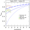 |
Fig. 15. Total fraction of obscured AGN with log NH > 22 vs. redshift observed in different X-ray samples of low-luminosity AGN (log LX ≈ 42.5; see text for details). Model curves are as in Fig. 14. The model with γ = 2 and θtorus = 45° (thick dashed blue line) provides a reasonable representation of the data. |
– Similarly to what is found by recent numerical simulations, our results suggest that 80–90% of SMBHs in the early Universe (z > 6 − 8) are hidden to our view, largely because of the ISM in their hosts. This would prevent standard UV-rest color selection for most SMBHs growing at early epochs.
Discovering hidden SMBHs in the early Universe and testing whether they are obscured by their host ISM are extremely challenging tasks, which may nonetheless be tackled efficiently with state-of-the-art or forthcoming facilities. For example, spatially resolved maps of emission line ratios at rest-UV, optical, and FIR wavelengths are all promising tools that rely on data from the VLT (in the future E-ELT), JWST, and ALMA, respectively. In addition, the diffuse, hard X-ray glow expected from the interaction of central AGN photons with the global galaxy-scale ISM may be resolved by next-generation imaging X-ray missions if these are designed to have sub-arcsec resolution optics.
Acknowledgments
We acknowledge financial contribution from the agreement ASI-INAF n. 2017-14-H.O. KI acknowledges support by the Spanish MCINN under grant PID2019-105510GB-C33/AEI/10.13039/501100011033 and “Unit of excellence María de Maeztu 2020–2023” awarded to ICCUB (CEX2019-000918-M). SM acknowledges funding from the INAF “Progetti di Ricerca di Rilevante Interesse Nazionale” (PRIN), Bando 2019 (project: “Piercing through the clouds: a multiwavelength study of obscured accretion in nearby supermassive black holes”). We finally thank the referee for their useful and insightful comments.
References
- Aihara, H., Arimoto, N., Armstrong, R., et al. 2018, PASJ, 70, S4 [NASA ADS] [Google Scholar]
- Aird, J., Coil, A. L., Georgakakis, A., et al. 2015, MNRAS, 451, 1892 [Google Scholar]
- Allen, R. J., Kacprzak, G. G., Glazebrook, K., et al. 2017, ApJ, 834, L11 [NASA ADS] [CrossRef] [Google Scholar]
- Aravena, M., Boogaard, L., Gónzalez-López, J., et al. 2020, ApJ, 901, 79 [NASA ADS] [CrossRef] [Google Scholar]
- Baloković, M., Brightman, M., Harrison, F. A., et al. 2018, ApJ, 854, 42 [Google Scholar]
- Barnett, R., Warren, S. J., Banerji, M., et al. 2015, A&A, 575, A31 [NASA ADS] [CrossRef] [EDP Sciences] [Google Scholar]
- Beckwith, S. V. W., Stiavelli, M., Koekemoer, A. M., et al. 2006, AJ, 132, 1729 [Google Scholar]
- Béthermin, M., Fudamoto, Y., Ginolfi, M., et al. 2020, A&A, 643, A2 [Google Scholar]
- Bianchini, F., Fabbian, G., Lapi, A., et al. 2019, ApJ, 871, 136 [CrossRef] [Google Scholar]
- Bigiel, F., & Blitz, L. 2012, ApJ, 756, 183 [Google Scholar]
- Bischetti, M., Maiolino, R., Carniani, S., et al. 2019, A&A, 630, A59 [NASA ADS] [CrossRef] [EDP Sciences] [Google Scholar]
- Bock, D. C. J., Bolatto, A. D., Hawkins, D. W., et al. 2006, SPIE Conf. Ser., 6267 [Google Scholar]
- Bolatto, A. D., Wong, T., Utomo, D., et al. 2017, ApJ, 846, 159 [Google Scholar]
- Boogaard, L. A., van der Werf, P., Weiss, A., et al. 2020, ApJ, 902, 109 [NASA ADS] [CrossRef] [Google Scholar]
- Bouché, N., Carfantan, H., Schroetter, I., Michel-Dansac, L., & Contini, T. 2015, AJ, 150, 92 [Google Scholar]
- Buchner, J., Georgakakis, A., Nandra, K., et al. 2015, ApJ, 802, 89 [Google Scholar]
- Buchner, J., Schulze, S., & Bauer, F. E. 2017, MNRAS, 464, 4545 [NASA ADS] [CrossRef] [Google Scholar]
- Buchner, J., Brightman, M., Nandra, K., Nikutta, R., & Bauer, F. E. 2019, A&A, 629, A16 [NASA ADS] [CrossRef] [EDP Sciences] [Google Scholar]
- Burlon, D., Ajello, M., Greiner, J., et al. 2011, ApJ, 728, 58 [Google Scholar]
- Calistro Rivera, G., Hodge, J. A., Smail, I., et al. 2018, ApJ, 863, 56 [Google Scholar]
- Calura, F., Jimenez, R., Panter, B., Matteucci, F., & Heavens, A. F. 2008, ApJ, 682, 252 [NASA ADS] [CrossRef] [Google Scholar]
- Calura, F., Gilli, R., Vignali, C., et al. 2014, MNRAS, 438, 2765 [NASA ADS] [CrossRef] [Google Scholar]
- Calura, F., Pozzi, F., Cresci, G., et al. 2017, MNRAS, 465, 54 [Google Scholar]
- Cazzoli, S., Arribas, S., Maiolino, R., & Colina, L. 2016, A&A, 590, A125 [NASA ADS] [CrossRef] [EDP Sciences] [Google Scholar]
- Chabrier, G. 2003, PASP, 115, 763 [Google Scholar]
- Circosta, C., Vignali, C., Gilli, R., et al. 2019, A&A, 623, A172 [NASA ADS] [CrossRef] [EDP Sciences] [Google Scholar]
- Combes, F., García-Burillo, S., Audibert, A., et al. 2019, A&A, 623, A79 [NASA ADS] [CrossRef] [EDP Sciences] [Google Scholar]
- da Cunha, E., Charlot, S., & Elbaz, D. 2008, MNRAS, 388, 1595 [Google Scholar]
- da Cunha, E., Walter, F., Smail, I. R., et al. 2015, ApJ, 806, 110 [Google Scholar]
- D’Amato, Q., Gilli, R., Vignali, C., et al. 2020, A&A, 636, A37 [NASA ADS] [CrossRef] [EDP Sciences] [Google Scholar]
- Davies, R., Esposito, S., Schmid, H. M., et al. 2018, in Ground-based and Airborne Instrumentation for Astronomy VII, eds. C. J. Evans, L. Simard, & H. Takami, SPIE Conf. Ser., 10702, 1070209 [Google Scholar]
- Decarli, R., Walter, F., Venemans, B. P., et al. 2018, ApJ, 854, 97 [Google Scholar]
- Decarli, R., Walter, F., Gónzalez-López, J., et al. 2019, ApJ, 882, 138 [Google Scholar]
- Dessauges-Zavadsky, M., Richard, J., Combes, F., et al. 2019, Nat. Astron., 3, 1115 [NASA ADS] [CrossRef] [Google Scholar]
- De Vis, P., Jones, A., Viaene, S., et al. 2019, A&A, 623, A5 [NASA ADS] [CrossRef] [EDP Sciences] [Google Scholar]
- Di Mascia, F., Gallerani, S., Behrens, C., et al. 2021, MNRAS, 503, 2349 [NASA ADS] [CrossRef] [Google Scholar]
- Díaz-Santos, T., Armus, L., Charmandaris, V., et al. 2017, ApJ, 846, 32 [Google Scholar]
- Dunne, L., Eales, S., Edmunds, M., et al. 2000, MNRAS, 315, 115 [Google Scholar]
- Elmegreen, B. G., & Elmegreen, D. M. 2006, ApJ, 650, 644 [CrossRef] [Google Scholar]
- Fabbiano, G., Elvis, M., Paggi, A., et al. 2017, ApJ, 842, L4 [NASA ADS] [CrossRef] [Google Scholar]
- Feltre, A., Charlot, S., & Gutkin, J. 2016, MNRAS, 456, 3354 [Google Scholar]
- Feng, Y., Di-Matteo, T., Croft, R. A., et al. 2016, MNRAS, 455, 2778 [NASA ADS] [CrossRef] [Google Scholar]
- Fontana, A., Santini, P., Grazian, A., et al. 2009, A&A, 501, 15 [NASA ADS] [CrossRef] [EDP Sciences] [Google Scholar]
- Fujimoto, S., Ouchi, M., Shibuya, T., & Nagai, H. 2017, ApJ, 850, 83 [Google Scholar]
- Fujimoto, S., Silverman, J. D., Bethermin, M., et al. 2020, ApJ, 900, 1 [Google Scholar]
- García-Burillo, S., Combes, F., Ramos Almeida, C., et al. 2019, A&A, 632, A61 [Google Scholar]
- Gilli, R., Comastri, A., & Hasinger, G. 2007, A&A, 463, 79 [NASA ADS] [CrossRef] [EDP Sciences] [Google Scholar]
- Gilli, R., Norman, C., Vignali, C., et al. 2014, A&A, 562, A67 [NASA ADS] [CrossRef] [EDP Sciences] [Google Scholar]
- Ginolfi, M., Jones, G. C., Béthermin, M., et al. 2020, A&A, 633, A90 [NASA ADS] [CrossRef] [EDP Sciences] [Google Scholar]
- Girelli, G., Bolzonella, M., & Cimatti, A. 2019, A&A, 632, A80 [NASA ADS] [CrossRef] [EDP Sciences] [Google Scholar]
- Graciá-Carpio, J., Sturm, E., Hailey-Dunsheath, S., et al. 2011, ApJ, 728, L7 [Google Scholar]
- Grazian, A., Fontana, A., Santini, P., et al. 2015, A&A, 575, A96 [NASA ADS] [CrossRef] [EDP Sciences] [Google Scholar]
- Grogin, N. A., Kocevski, D. D., Faber, S. M., et al. 2011, ApJS, 197, 35 [NASA ADS] [CrossRef] [Google Scholar]
- Hasinger, G. 2008, A&A, 490, 905 [NASA ADS] [CrossRef] [EDP Sciences] [Google Scholar]
- Hickox, R. C., & Alexander, D. M. 2018, ARA&A, 56, 625 [Google Scholar]
- Hodge, J. A., & da Cunha, E. 2020, R. Soc. Open Sci., 7, 200556 [NASA ADS] [CrossRef] [Google Scholar]
- Hodge, J. A., Smail, I., Walter, F., et al. 2019, ApJ, 876, 130 [Google Scholar]
- Hughes, D. H., Dunlop, J. S., & Rawlings, S. 1997, MNRAS, 289, 766 [NASA ADS] [CrossRef] [Google Scholar]
- Illingworth, G. D., Magee, D., Oesch, P. A., et al. 2013, ApJS, 209, 6 [Google Scholar]
- Iwasawa, K., Wilson, A. S., Fabian, A. C., & Young, A. J. 2003, MNRAS, 345, 369 [NASA ADS] [CrossRef] [Google Scholar]
- Iwasawa, K., Gilli, R., Vignali, C., et al. 2012, A&A, 546, A84 [NASA ADS] [CrossRef] [EDP Sciences] [Google Scholar]
- Iwasawa, K., Comastri, A., Vignali, C., et al. 2020, A&A, 639, A51 [NASA ADS] [CrossRef] [EDP Sciences] [Google Scholar]
- Izumi, T., Onoue, M., Shirakata, H., et al. 2018, PASJ, 70, 36 [NASA ADS] [Google Scholar]
- Izumi, T., Onoue, M., Matsuoka, Y., et al. 2019, PASJ, 71, 111 [CrossRef] [Google Scholar]
- Jones, M. L., Parker, K., Fabbiano, G., et al. 2021, ApJ, 910, 19 [NASA ADS] [CrossRef] [Google Scholar]
- Koekemoer, A. M., Faber, S. M., Ferguson, H. C., et al. 2011, ApJS, 197, 36 [NASA ADS] [CrossRef] [Google Scholar]
- La Franca, F., Fiore, F., Comastri, A., et al. 2005, ApJ, 635, 864 [NASA ADS] [CrossRef] [Google Scholar]
- Lambrides, E. L., Chiaberge, M., Heckman, T., et al. 2020, ApJ, 897, 160 [Google Scholar]
- Lang, P., Schinnerer, E., Smail, I., et al. 2019, ApJ, 879, 54 [Google Scholar]
- Lanzuisi, G., Delvecchio, I., Berta, S., et al. 2017, A&A, 602, A123 [NASA ADS] [CrossRef] [EDP Sciences] [Google Scholar]
- Lanzuisi, G., Civano, F., Marchesi, S., et al. 2018, MNRAS, 480, 2578 [Google Scholar]
- Leauthaud, A., Massey, R., Kneib, J.-P., et al. 2007, ApJS, 172, 219 [NASA ADS] [CrossRef] [Google Scholar]
- Le Fèvre, O., Béthermin, M., Faisst, A., et al. 2020, A&A, 643, A1 [Google Scholar]
- Lehmer, B. D., Brandt, W. N., Alexander, D. M., et al. 2005, ApJS, 161, 21 [NASA ADS] [CrossRef] [Google Scholar]
- Leipski, C., Meisenheimer, K., Walter, F., et al. 2014, ApJ, 785, 154 [Google Scholar]
- Lequeux, J., Peimbert, M., Rayo, J. F., Serrano, A., & Torres-Peimbert, S. 1979, A&A, 80, 155 [Google Scholar]
- Liu, T., Tozzi, P., Wang, J.-X., et al. 2017, ApJS, 232, 8 [NASA ADS] [CrossRef] [Google Scholar]
- Liu, D., Schinnerer, E., Groves, B., et al. 2019, ApJ, 887, 235 [Google Scholar]
- Luo, B., Brandt, W. N., Xue, Y. Q., et al. 2017, ApJS, 228, 2 [Google Scholar]
- Lupi, A., Volonteri, M., Decarli, R., Bovino, S., & Silk, J. 2022, MNRAS, 510, 5760 [NASA ADS] [CrossRef] [Google Scholar]
- Lusso, E., Hennawi, J. F., Comastri, A., et al. 2013, ApJ, 777, 86 [Google Scholar]
- Ma, J., Elvis, M., Fabbiano, G., et al. 2020, ApJ, 900, 164 [NASA ADS] [CrossRef] [Google Scholar]
- Magdis, G. E., Daddi, E., Béthermin, M., et al. 2012, ApJ, 760, 6 [NASA ADS] [CrossRef] [Google Scholar]
- Maiolino, R., & Mannucci, F. 2019, A&ARv, 27, 3 [Google Scholar]
- Maiolino, R., Shemmer, O., Imanishi, M., et al. 2007, A&A, 468, 979 [NASA ADS] [CrossRef] [EDP Sciences] [Google Scholar]
- Maiolino, R., Nagao, T., Grazian, A., et al. 2008, A&A, 488, 463 [NASA ADS] [CrossRef] [EDP Sciences] [Google Scholar]
- Maksym, W. P., Fabbiano, G., Elvis, M., et al. 2017, ApJ, 844, 69 [NASA ADS] [CrossRef] [Google Scholar]
- Malhotra, S., Kaufman, M. J., Hollenbach, D., et al. 2001, ApJ, 561, 766 [Google Scholar]
- Marchesi, S., Ajello, M., Marcotulli, L., et al. 2018, ApJ, 854, 49 [Google Scholar]
- Marchesi, S., Ajello, M., Zhao, X., et al. 2019, ApJ, 872, 8 [Google Scholar]
- Marchesi, S., Gilli, R., Lanzuisi, G., et al. 2020, A&A, 642, A184 [EDP Sciences] [Google Scholar]
- Marshall, M. A., Mechtley, M., Windhorst, R. A., et al. 2020, ApJ, 900, 21 [NASA ADS] [CrossRef] [Google Scholar]
- Masoura, V. A., Mountrichas, G., Georgantopoulos, I., & Plionis, M. 2021, A&A, 646, A167 [EDP Sciences] [Google Scholar]
- Matsuoka, Y., Onoue, M., Kashikawa, N., et al. 2016, ApJ, 828, 26 [Google Scholar]
- Matsuoka, Y., Iwasawa, K., Onoue, M., et al. 2019, ApJ, 883, 183 [Google Scholar]
- Mechtley, M., Windhorst, R. A., Ryan, R. E., et al. 2012, ApJ, 756, L38 [NASA ADS] [CrossRef] [Google Scholar]
- Mignoli, M., Feltre, A., Bongiorno, A., et al. 2019, A&A, 626, A9 [NASA ADS] [CrossRef] [EDP Sciences] [Google Scholar]
- Miville-Deschênes, M.-A., Murray, N., & Lee, E. J. 2017, ApJ, 834, 57 [Google Scholar]
- Mortlock, A., Conselice, C. J., Hartley, W. G., et al. 2013, MNRAS, 433, 1185 [NASA ADS] [CrossRef] [Google Scholar]
- Mushotzky, R. 2018, in Space Telescopes and Instrumentation 2018: Ultraviolet to Gamma Ray, eds. J. W. A. den Herder, S. Nikzad, & K. Nakazawa, SPIE Conf. Ser., 10699, 1069929 [NASA ADS] [Google Scholar]
- Nakajima, K., Fletcher, T., Ellis, R. S., Robertson, B. E., & Iwata, I. 2018a, MNRAS, 477, 2098 [NASA ADS] [CrossRef] [Google Scholar]
- Nakajima, K., Schaerer, D., Le Fèvre, O., et al. 2018b, A&A, 612, A94 [NASA ADS] [CrossRef] [EDP Sciences] [Google Scholar]
- Nandra, K., Barret, D., Barcons, X., et al. 2013, ArXiv e-prints [arXiv:1306.2307] [Google Scholar]
- Nanni, R., Gilli, R., Vignali, C., et al. 2018, A&A, 614, A121 [NASA ADS] [CrossRef] [EDP Sciences] [Google Scholar]
- Nenkova, M., Sirocky, M. M., Ivezić, Ž., & Elitzur, M. 2008, ApJ, 685, 147 [Google Scholar]
- Netzer, H. 2015, ARA&A, 53, 365 [Google Scholar]
- Ni, Y., Di Matteo, T., Gilli, R., et al. 2020, MNRAS, 495, 2135 [NASA ADS] [CrossRef] [Google Scholar]
- Peng, C. Y., Ho, L. C., Impey, C. D., & Rix, H.-W. 2002, AJ, 124, 266 [Google Scholar]
- Peng, C. Y., Ho, L. C., Impey, C. D., & Rix, H.-W. 2010, AJ, 139, 2097 [Google Scholar]
- Perley, D. A., Krühler, T., Schulze, S., et al. 2016, ApJ, 817, 7 [Google Scholar]
- Pierre, M., Pacaud, F., Adami, C., et al. 2016, A&A, 592, A1 [NASA ADS] [CrossRef] [EDP Sciences] [Google Scholar]
- Planck Collaboration XIII. 2016, A&A, 594, A13 [NASA ADS] [CrossRef] [EDP Sciences] [Google Scholar]
- Popping, G., Pillepich, A., Calistro Rivera, G., et al. 2022, MNRAS, 510, 3321 [CrossRef] [Google Scholar]
- Pozzi, F., Calura, F., Fudamoto, Y., et al. 2021, A&A, 653, A84 [NASA ADS] [CrossRef] [EDP Sciences] [Google Scholar]
- Ramos Almeida, C., & Ricci, C. 2017, Nat. Astron., 1, 679 [Google Scholar]
- Rémy-Ruyer, A., Madden, S. C., Galliano, F., et al. 2014, A&A, 563, A31 [Google Scholar]
- Ricci, C., Trakhtenbrot, B., Koss, M. J., et al. 2017, Nature, 549, 488 [NASA ADS] [CrossRef] [Google Scholar]
- Richards, G. T., Strauss, M. A., Fan, X., et al. 2006, AJ, 131, 2766 [Google Scholar]
- Risaliti, G., Maiolino, R., & Salvati, M. 1999, ApJ, 522, 157 [Google Scholar]
- Roberts-Borsani, G. W., Saintonge, A., Masters, K. L., & Stark, D. V. 2020, MNRAS, 493, 3081 [Google Scholar]
- Santini, P., Ferguson, H. C., Fontana, A., et al. 2015, ApJ, 801, 97 [Google Scholar]
- Scoville, N., Aussel, H., Brusa, M., et al. 2007, ApJS, 172, 1 [Google Scholar]
- Scoville, N., Sheth, K., Aussel, H., et al. 2016, ApJ, 820, 83 [Google Scholar]
- Scoville, N., Lee, N., Vanden Bout, P., et al. 2017, ApJ, 837, 150 [Google Scholar]
- Shibuya, T., Ouchi, M., Kubo, M., & Harikane, Y. 2016, ApJ, 821, 72 [NASA ADS] [CrossRef] [Google Scholar]
- Shibuya, T., Ouchi, M., Harikane, Y., & Nakajima, K. 2019, ApJ, 871, 164 [NASA ADS] [CrossRef] [Google Scholar]
- Sobral, D., Matthee, J., Darvish, B., et al. 2018, MNRAS, 477, 2817 [Google Scholar]
- Stacey, G. J., Geis, N., Genzel, R., et al. 1991, ApJ, 373, 423 [NASA ADS] [CrossRef] [Google Scholar]
- Stacey, G. J., Hailey-Dunsheath, S., Ferkinhoff, C., et al. 2010, ApJ, 724, 957 [NASA ADS] [CrossRef] [Google Scholar]
- Stefanon, M., Bouwens, R. J., Labbé, I., et al. 2021, ApJ, 922, 29 [NASA ADS] [CrossRef] [Google Scholar]
- Suzuki, T. L., Onodera, M., Kodama, T., et al. 2021, ApJ, 908, 15 [NASA ADS] [CrossRef] [Google Scholar]
- Tacconi, L. J., Genzel, R., Saintonge, A., et al. 2018, ApJ, 853, 179 [Google Scholar]
- Thatte, N., Tecza, M., Schnetler, H., et al. 2021, The Messenger, 182, 7 [NASA ADS] [Google Scholar]
- The Lynx Team 2018, ArXiv e-prints [arXiv:1809.09642] [Google Scholar]
- Torres-Albà, N., Marchesi, S., Zhao, X., et al. 2021, ApJ, 922, 252 [CrossRef] [Google Scholar]
- Torrey, P., Vogelsberger, M., Marinacci, F., et al. 2019, MNRAS, 484, 5587 [NASA ADS] [Google Scholar]
- Tozzi, P., Gilli, R., Mainieri, V., et al. 2006, A&A, 451, 457 [NASA ADS] [CrossRef] [EDP Sciences] [Google Scholar]
- Trebitsch, M., Volonteri, M., & Dubois, Y. 2019, MNRAS, 487, 819 [CrossRef] [Google Scholar]
- Treister, E., & Urry, C. M. 2006, ApJ, 652, L79 [NASA ADS] [CrossRef] [Google Scholar]
- Tremonti, C. A., Heckman, T. M., Kauffmann, G., et al. 2004, ApJ, 613, 898 [Google Scholar]
- Ueda, Y., Akiyama, M., Hasinger, G., Miyaji, T., & Watson, M. G. 2014, ApJ, 786, 104 [Google Scholar]
- Vallini, L., Pallottini, A., Ferrara, A., et al. 2018, MNRAS, 473, 271 [NASA ADS] [CrossRef] [Google Scholar]
- Vallini, L., Tielens, A. G. G. M., Pallottini, A., et al. 2019, MNRAS, 490, 4502 [CrossRef] [Google Scholar]
- van der Wel, A., Bell, E. F., Häussler, B., et al. 2012, ApJS, 203, 24 [NASA ADS] [CrossRef] [Google Scholar]
- Venemans, B. P., Decarli, R., Walter, F., et al. 2018, ApJ, 866, 159 [Google Scholar]
- Venemans, B. P., Walter, F., Neeleman, M., et al. 2020, ApJ, 904, 130 [Google Scholar]
- Venturi, G., Nardini, E., Marconi, A., et al. 2018, A&A, 619, A74 [NASA ADS] [CrossRef] [EDP Sciences] [Google Scholar]
- Vito, F., Brandt, W. N., Yang, G., et al. 2018, MNRAS, 473, 2378 [Google Scholar]
- Vogelsberger, M., Genel, S., Springel, V., et al. 2014, MNRAS, 444, 1518 [Google Scholar]
- Walter, F., Carilli, C., Neeleman, M., et al. 2020, ApJ, 902, 111 [Google Scholar]
- Walter, F., Neeleman, M., Decarli, R., et al. 2022, ApJ, 927, 21 [NASA ADS] [CrossRef] [Google Scholar]
- Whitney, A., Ferreira, L., Conselice, C. J., & Duncan, K. 2021, ApJ, 919, 139 [NASA ADS] [CrossRef] [Google Scholar]
- Willingale, R., Starling, R. L. C., Beardmore, A. P., Tanvir, N. R., & O’Brien, P. T. 2013, MNRAS, 431, 394 [Google Scholar]
- Wolfire, M. G., McKee, C. F., Hollenbach, D., & Tielens, A. G. G. M. 2003, ApJ, 587, 278 [Google Scholar]
- Wright, E. L., Eisenhardt, P. R. M., Mainzer, A. K., et al. 2010, AJ, 140, 1868 [Google Scholar]
- Yan, W., Hickox, R. C., Chen, C.-T. J., et al. 2021, ApJ, 914, 83 [NASA ADS] [CrossRef] [Google Scholar]
- Yang, G., Chen, C. T. J., Vito, F., et al. 2017, ApJ, 842, 72 [NASA ADS] [CrossRef] [Google Scholar]
- Zanella, A., Daddi, E., Magdis, G., et al. 2018, MNRAS, 481, 1976 [Google Scholar]
- Zappacosta, L., Comastri, A., Civano, F., et al. 2018, ApJ, 854, 33 [Google Scholar]
- Zhao, X., Marchesi, S., Ajello, M., et al. 2021, A&A, 650, A57 [NASA ADS] [CrossRef] [EDP Sciences] [Google Scholar]
All Tables
Summary of the galaxy samples with M* > 1010 M⊙ and reliable size estimates used in this work (see text for details).
All Figures
|
Fig. 1. Estimated dust mass vs. redshift for the considered galaxy samples as labeled. For high-z QSO hosts, dust masses have been estimated from Eq. (2) assuming Td = 47 K if Tmin < 47 K or Td = 1.2Tmin if Tmin > 47 K (see text for details). For the ASPECS and COSMOS samples, the original dust masses derived through SED-fitting (MAGPHYS) are plotted as open symbols, and those derived from a single MBB with Td = 47 K as filled symbols. The dashed curve shows the dust mass limit corresponding to a flux density of 30 μJy at 1.2 mm (i.e., the ∼3σ detection limit in ASPECS) from Eq. (2) assuming Td = 47 K. |
| In the text | |
|
Fig. 2. Summary chart of the ISM mass and size proxies available for our samples (green shaded cells). Dark green ticks mark those proxies that have been used in the final ISM column density estimates (see Sect. 3.1 and 3.2 for details). |
| In the text | |
|
Fig. 3. Distribution of the minimum blackbody temperature Tmin required to explain the observed 1.2 mm brightness of z ∼ 6 QSOs. The Venemans et al. (2020) and SHELLQs samples are shown in brown and purple, respectively. Note that the 1.2 mm emission on approximately kiloparsec scales of a few bright objects can only be reproduced by hot dust with Td > 50 − 100 K. We used Td = 47 K, a standard reference value used in the literature (e.g., Venemans et al. 2020), to derive the dust masses of all QSOs with Tmin < 47 K. For hotter systems, we used Td = 1.2Tmin (see text for details). |
| In the text | |
|
Fig. 4. Comparison between ISM mass (left), size (center) and column density (right) as derived from [C II] and dust continuum observations for the z ∼ 6 QSO samples. The ISM masses derived with the two methods agree for δGDR = 200. The [C II]-based sizes are on average ∼1.5 times larger than the dust continuum sizes. The total ISM column densities are on average higher for the dust continuum method, owing to the smaller sizes measured. Three sources with upper limits to their continuum size in the Venemans et al. (2020) sample are marked with arrows in the central and right panels. One SHELLQs source is not detected in the continuum, and is shown with an arrow in the left and right panels. For this and for another source in the same sample (both marked with large open squares in the central and right panels), the size could not be estimated, so we assumed it equal to the median of the sample. |
| In the text | |
|
Fig. 5. Edge-on sketch of the adopted disk galaxy geometry. The darker shading reflects the higher ISM density of the assumed exponential profile. |
| In the text | |
|
Fig. 6. Comparison between the ISM column densities toward the nucleus of ASPECS galaxies derived by assuming a fixed, average galaxy orientation (θ* = 57.3 deg) vs. those derived from individual galaxy orientations θ. The inset shows the distribution of the Δlog NH, ISM values: a Gaussian fit (dashed curve) is centered at about 0 (dotted line) and has rms ∼ 0.15 dex. |
| In the text | |
|
Fig. 7. Variation of the average number of ISM clouds along a given line of sight to the nucleus as a function of the viewing angle θ (90° is edge on) for a typical massive galaxy with Mgas ∼ 1010 M⊙ at z = 2.5. |
| In the text | |
|
Fig. 8. Obscured AGN fraction as a function of τ, the average number of clouds along edge-on views, and ϵ, the ratio between the average number of clouds seen face-on vs. edge-on. |
| In the text | |
|
Fig. 9. ISM column density vs. redshift for different samples of M* > 1010 M⊙ galaxies as labeled. For ASPECS and COSMOS z ∼ 3.3 galaxies, ISM masses were derived from dust masses, and ISM sizes from UV/optical stellar sizes. For ALPINE galaxies and for z ∼ 6 QSO hosts both ISM masses and sizes were derived from [C II] data. For comparison, we also show for the ALPINE sample the results obtained using ISM masses derived from dust mass and ISM sizes derived from UV/optical stellar sizes (green open pentagons; see text for details). The upper bound of the light blue shaded area shows the median NH values obtained for the different samples (ASPECS was divided into two redshift bins). The lower bound shows the median NH values after including a conservative correction for incompleteness and observational biases (see Sect. 5.2). The NH ∝ (1 + z)4 solid curve is obtained by combining empirical trends for the gas mass and galaxy size and is normalized to NH = 1021 cm−2 at z = 0, which is consistent with the angle-averaged column density of the Milky Way (Willingale et al. 2013) and with the upper limit to the median column density of local massive galaxies as derived from the EDGE-CALIFA survey (Bolatto et al. 2017; big square at z = 0.1). The long-dashed curve running through the light-blue shaded area corresponds to (1 + z)3.3. The gold shaded area is from Buchner et al. (2017) as derived from the Illustris-1 simulation: lower and upper bounds are for galaxies with M* > 1010 M⊙ and M* > 1011 M⊙, respectively. The horizontal dashed line shows the column density corresponding to Compton-thick absorption. |
| In the text | |
|
Fig. 10. Comparison between the evolution of the median column density of the ISM (light blue shaded area and black dashed curve – same meaning as in Fig. 9) and of the median absorption column density measured in different AGN samples through X-ray spectroscopy (see text for details). At z ≳ 1.5 − 2 the ISM column density becomes comparable to that measured in the X-rays. |
| In the text | |
|
Fig. 11. Expected redshift evolution of the ISM-obscured AGN fraction. Blue curves consider a slower (γ = 2) increase with redshift of the characteristic cloud density Σc, *. Red curves assume a faster increase (γ = 3). Labels refer to different thresholds in log column density (see text for details). |
| In the text | |
|
Fig. 12. Edge-on view of the considered geometry for the ISM clouds and the torus (not to scale). |
| In the text | |
|
Fig. 13. Total fraction of obscured AGN with log NH > 22 (left panel) and log NH > 23 (right panel) vs. redshift for different combinations of large-scale (ISM) and small-scale (torus) obscuration. All curves are for δ = 3.3 and ϵ = 0.25. The characteristic surface density Σc, * of ISM clouds is assumed to evolve as ∝(1 + z)γ, with γ = 2 (blue curves) or γ = 3 (red curves). Short dashed lines refer to ISM-only obscuration (i.e., no torus considered, as in Fig. 11). Long dashed and solid lines show the total obscured AGN fraction when adding a torus with half-opening angle θtorus = 45° and 60°, respectively. The horizontal dotted lines show the obscured AGN fraction expected by torus-only obscuration. |
| In the text | |
|
Fig. 14. Total fraction of obscured AGN with log NH > 22 (left panel) and log NH > 23 (right panel) vs. redshift measured in different X-ray samples (see labels) and compared with model curves of large-scale (ISM) plus small-scale (torus) obscuration. Only samples with median log LX ≈ 44 have been considered here (see text for details). Curves have the same meaning as in Fig. 13. The model with γ = 2 and θtorus = 60° (thick solid blue line) provides a good representation of the data. |
| In the text | |
|
Fig. 15. Total fraction of obscured AGN with log NH > 22 vs. redshift observed in different X-ray samples of low-luminosity AGN (log LX ≈ 42.5; see text for details). Model curves are as in Fig. 14. The model with γ = 2 and θtorus = 45° (thick dashed blue line) provides a reasonable representation of the data. |
| In the text | |
Current usage metrics show cumulative count of Article Views (full-text article views including HTML views, PDF and ePub downloads, according to the available data) and Abstracts Views on Vision4Press platform.
Data correspond to usage on the plateform after 2015. The current usage metrics is available 48-96 hours after online publication and is updated daily on week days.
Initial download of the metrics may take a while.