| Issue |
A&A
Volume 666, October 2022
|
|
|---|---|---|
| Article Number | A197 | |
| Number of page(s) | 13 | |
| Section | Interstellar and circumstellar matter | |
| DOI | https://doi.org/10.1051/0004-6361/202243297 | |
| Published online | 28 October 2022 | |
Closing of the astrotail
Space Research Centre,
Polish Academy of Sciences Bartycka 18A,
00-716
Warsaw, Poland
e-mail: This email address is being protected from spambots. You need JavaScript enabled to view it.
Received:
9
February
2022
Accepted:
31
July
2022
Abstract
Context. The structure of astrospheres depends on the interaction between the host star and the surrounding interstellar medium (ISM). Observations of astrospheres offer new opportunities to learn about the details of this interaction.
Aims. The aim of this work is to study the global structure of astrospheres, concentrating on the case of strong interstellar magnetic field and low relative velocity between the star and the ISM.
Methods. We used a simple magnetohydrodynamical numerical code to simulate the interaction between the stellar wind and the ISM, using different assumptions about the interstellar magnetic field strength, the velocity of the star, and the parameters of the interstellar medium. From the resulting time-stationary solutions, we derived the mass flux distribution of the stellar plasma inside the astrosphere, with particular attention to the flow topology.
Results. We find that the tube-like topology of the astrosphere can occur for an interstellar magnetic field strength of 7 µG (a realistic value in the Galactic disk region), provided that the velocity of the star relative to the ISM is low enough (0.5 km s−1 ). The two-stream structure of the stellar wind mass flow appears to some extent in all our models.
Key words: magnetohydrodynamics (MHD) / ISM: bubbles / ISM: magnetic fields / stars: solar-type
© A. Czechowski and J. Grygorczuk 2022
 Open Access article, published by EDP Sciences, under the terms of the Creative Commons Attribution License (https://creativecommons.org/licenses/by/4.0), which permits unrestricted use, distribution, and reproduction in any medium, provided the original work is properly cited.
This article is published in open access under the Subscribe-to-Open model. This email address is being protected from spambots. You need JavaScript enabled to view it. to support open access publication.
1 Introduction
Astrospheres are cavities in the interstellar plasma filled by the stellar wind of the host star. Their structures are expected to vary, depending on parameters like stellar wind strength, relative velocity between the star and the interstellar plasma, and strength and orientation of the interstellar magnetic field. Observations of astrospheres are by now numerous, using hydrogen Ly-α (see e.g. Wood 2004; Linsky & Wood 2014), other UV signals (Wood et al. 2016; Sahai & Chronopoulos 2010, and many others), and IR emissions from bow shock region (Decin et al. 2012). Theoretical studies include the magnetohydrodynamics (MHD) structure of astrospheres (Scherer et al. 2016, 2020), simulations of magnetised stellar wind bubbles around massive stars (Van Marle 2015; Meyer et al. 2014; Mackey et al. 2020) or double stars (Mueller & Juric 2021), and interactions of astrospheres with cosmic rays (Struminsky & Sadovski 2019). With improving means of observation, we may hope that more features of astrospheres will become accessible for study.
In a pioneering work, Parker (1961, 1963) described three astrosphere models: a closed but expanding bubble around a star at rest relative to the interstellar medium (ISM), a comet-like cavity for the moving star, and a tube-like structure with two stellar wind streams directed parallel and antiparallel to the interstellar magnetic field. Each of these models has a different topology. The comet-like possibility was given most attention because it might be applied to the heliosphere.
The aim of the present work is to study the model astrospheres in the region of parameter space in which the topology of the stellar plasma flow is likely to change. We use simple 3D MHD numerical time-stationary models, assuming different values of the parameters of the interstellar medium, in particular, the interstellar magnetic field strength and the speed of the interstellar plasma relative to the star, trying to determine the change from the single-tail to the two-stream topology. We restrict our attention to Sun-like stars.
We concentrate on the mass flux distribution inside the astrospheres. The mass flux was approximated by a finite number of flow lines, each representing the same fraction of the total flux.
The structure of the paper is as follows. Our methods are described in Sect. 2. Section 3 presents the results. Section 3.1 describes the two-stream structure of the plasma flow, Sect. 3.2 the flow structure at large distances downstream (by “downstream” we mean here the direction of the ISM flow), Sect. 3.3 discusses the effect of the magnetic field of the host star, and Sect. 3.4 the case when the neutral hydrogen density is close to zero. Section 4 contains the discussion and our conclusions.
2 Method
The model astrospheres we considered rely on MHD simulations of the interaction between the stellar wind and the interstellar medium. The code is a modification of the code used by Ratkiewicz et al. (1998), extended to include the neutral component of the interstellar medium (Ratkiewicz et al. 2002, the Warsaw model). Our modification permits including the neutral component in a simulation together with a self-adjusting iteration step, which speeds up the calculation.
The neutral component of the interstellar medium is treated as a background, with a constant number density and velocity. The stellar wind and the interstellar plasma interact with this background via charge exchange, but the effect of this interaction on the neutral component is not taken into account. This approximation is partly justified because the plasma density inside the astropause in most of our models is much lower than the interstellar density. For simplicity, we considered only the proton (hydrogen) component of the stellar wind and the interstellar medium. Mass loading of the stellar wind is absent from our models.
We restricted our attention to time-stationary solutions. We assumed that the stellar wind is spherically symmetric at the inner boundary of our region of calculations (a one-component stellar wind). The direction of the interstellar magnetic field, the number density, the temperature and flow direction of the interstellar plasma and initial velocity, the density, and the temperature of the stellar wind were the same for most simulations (see Table 1). The stellar magnetic field was neglected for most simulations: in these cases, the models are symmetric with respect to the (B, V) plane. For comparison, we included some examples in which the stellar magnetic field was taken into account, and some examples in which neutral hydrogen or the proton density in the ISM were set to a low value. The list of all our models is given in Table 2, and Table 3 lists the values of the Alfvénic Mach number and plasma β for the undisturbed ISM.
We used a system of coordinates (see Fig. 1) with the origin at the host star of the considered astrosphere. The x-axis is directed opposite to the direction of the stellar velocity relative to ISM, that is, along the ISM inflow direction into the astrosphere. The x- and y-axes belong to the (B, V) plane (the plane defined by the interstellar magnetic field B and the ISM flow velocity V relative to the star) and the z-axis completes the right-handed system. In the numerical simulation, we used a spherical grid, logarithmic in distance from the star (constant steps in log(r), 348 grid points, and a range from 30 AU to 5900 AU) and uniform in angles (90 grid points for the polar angle, from 1° to 179°, and 180 grid points for the azimuthal angle, from 1° to 359°) with –x as the polar axis.
To present our results, we also used the astrospheric longitude (ϕ) and latitude (θ) angles, with the (B, V) plane considered as the equator plane. The astrospheric latitude θ is positive for z > 0. The astrospheric longitude ϕ is counted from the x-axis (see Fig. 1).
The boundary conditions are defined as follows. At the outer boundary (the sphere of radius 5900 AU with the centre at the star), we used the parameters of the undisturbed interstellar plasma. The direction of the plasma flow is parallel to the x-axis. The direction (bx, by, bz) of the interstellar magnetic field and the plasma temperature TIS are given in Table 1. The magnetic field magnitude BIS, the plasma speed VIS, and the plasma number density np,IS of the undisturbed ISM are listed in Table 2.
At the inner boundary (the sphere with a radius of 30 AU), the boundary conditions are defined by the parameters of the stellar wind of the host star. To derive the boundary values, we assumed that in the region just outside the inner boundary, we can use a spherically symmetric model of the stellar wind, with constant speed and temperature, and the number density behaving as 1/r2 , where r is the distance from the host star. The speed VSW, the temperature TSW, and the number density  (the latter at 1 AU from the star) are given in Table 1.
In most simulations, the magnetic field at the inner boundary is assumed equal to zero. When the magnetic field of the host star is taken into account, we defined the boundary condition using the analytical model described in Sect. 3.3.
The parameters of the neutral component, that is, number density, velocity, and temperature, were constant throughout the calculation domain. This includes the two boundaries.
The aim of the present work is to study the mass flux distribution of the wind from the host star inside the astrosphere. Our method is to approximate the mass flux by a finite set of plasma flow lines.
For each MHD solution, we calculated numerically (using the Runge–Kutta method with an adaptive step size) the plasma flow lines starting from a sphere with the centre at the star and situated inside the stellar wind termination shock. The initial points of the flow lines were distributed uniformly over this sphere. In all models considered here, the stellar wind was spherically symmetric near the star. We therefore assumed that each of these flow lines corresponds to the same portion of the total flux of the stellar wind. The mass flux across some surface element inside the astrosphere can then be estimated by counting the number of flow lines passing through this surface. For trajectories crossing the surface more than once, we used the last of the crossings.
The distribution of mass flux at the distance r from the star is then approximately represented by the distribution of the points at which the flow lines cross the spherical surface of radius r surrounding the star. Varying the radius r of the sphere, we can follow the evolution of the mass flux with the distance from the star. To study the flow far downstream from the star, we used the planes perpendicular to the x-axis instead of spheres with the centre at the star.
If the astrosphere has a single tail, we expect to obtain (at a distance far enough from the termination shock) the crossing points distributed over a singly connected region. A tube-like astrosphere would correspond to the case of two clearly separated regions, each representing one plasma stream. Two plasma streams may also coexist with a third (tail) component of the flow.
In all calculations, we used Ntot = 9999 flow lines. When the parameters in Table 1 are used, the total proton flux from the host star is approximately Ftot = 8.5 × 1035 protons/s. N flow lines carry the flux F = N Ftot/Ntot protons s−1. In the following, we sometimes use for brevity “flux” for the number of flow lines (see Table 3 and the following discussion).
Model parameters, common values (bi = BIS,i/BIS ).
List of models.
Alfvénic Mach number and plasma β values for the models.
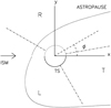 |
Fig. 1 Definition of our coordinate system. The termination shock and the astropause in the (B, V) plane (model 1: V = 2 km s−1, B = 3 µG case) are outlined. The x- and y-axes lie on the (B, V) plane. The x-axis is directed along the ISM inflow. The z-axis (not shown) completes the right-handed system. The angle ϕ (the astrospheric longitude) is counted from the x-axis. The astrospheric latitude θ is counted from the (B, V) plane. Dash-dotted lines show the limits in longitude of the R, L, and T sectors. |
3 Results
The results presented here describe the case of a solar-type star moving through different environments. In all our simulations, the interstellar magnetic field was inclined at the same angle (ϕ = 48.3°) to the velocity of the undisturbed ISM relative to the star. The speed of the ISM inflow V and the interstellar magnetic field strength B depend on the model. For B, we considered four cases: 3 µG, 7 µG, 10 µG, and 20 µG. The case of B = 20 µG, which is too high to be realistic outside of the Galactic bulge region, was included for comparison.
We expect that astrospheres with a tube-like topology are likely to appear when the velocity of the host star relative to the ISM is low. Observations and theoretical arguments (Belfort & Crovisier 1984; Marchal & Miville-Deschenes 2021) imply that very low values of this speed are not probable (V ≈ 26 km s−1 in the case of the Sun; Swaczyna et al. 2022). Therefore, we included also the cases with the ISM inflow speed V equal to 10 and 15 km s−1, searching for situations with a prominent two-stream structure of the astrospheric plasma flow.
In most of our simulations, the stellar magnetic field was neglected. When the stellar magnetic field was included, we assumed the rotation axis of the host star to be directed at θ = 47°, ϕ = 83° using our astrospheric latitude and longitude angles.
The neutral component of the interstellar medium was treated as a constant background. The speed Vis and the hydrogen density nH,IS were the same as in the undisturbed ISM far upstream of the astrosphere (see Table 2). In some calculations, the neutral background was effectively neglected by setting the hydrogen number density to a low value (nH,IS = 0.001 cm−3). We also considered some models in which the ISM proton density np,IS was reduced from the value of 0.06 cm−3 that was used in most calculations.
3.1 Evolution of the two-stream structure
The flow of the stellar wind plasma in most our models exhibits (to some degree) a two-stream structure, with two streams initially (i.e. before they turn towards the positive x-axis) directed approximately along or opposite to the interstellar magnetic field direction. A similar structure was obtained in our earlier work (Czechowski & Grygorczuk 2017). The two-stream structure arises because of the anisotropic pressure of the strong interstellar magnetic field and becomes more pronounced when the ISM inflow speed is low. This structure may persist throughout our region of calculation (the case of a strong interstellar magnetic field and low inflow speed) or acquire a strong tail component.
The two-stream structure is present in Fig. 2, which shows the selected flow lines (those staying near to the (B, V) plane) for two models: the V = 2 km s−1, B = 7 µG (upper panel) and V = 2 km s−1, B = 20 µG (lower panel). In the upper panel, the streams are not clearly separated from the tail component. The lower panel shows a purely two-stream flow. We use the designation of “R” (“rear” ) and “L” (“leading” ) streams, and “T” is used for the astrotail (Figs. 1 and 2).
More complete information about the flow is provided by Figs. 3 and 4. They show the distributions of the crossing points (in the astrospheric longitude-latitude plane) for the flow lines passing a sphere with a radius of 300 AU with the centre at the host star. In the upper plot of Fig. 3 (inflow speed V = 0.5 km s−1), the regions representing the R and L streams are separated from each other. In the lower panel (V = 2 km s−1), they are linked together, suggesting the existence of a weaker third component (the tail).
In Fig. 4, the inflow speed is higher (V = 10 km s−1). The upper plot shows the case (model 9) in which an ISM proton density of np,IS = 0.06 cm−3 as assumed in most simulations. The flux in the tail component is then not weak, and the R and L streams cannot be considered separate. The lower plot corresponds to the case in which the proton density is reduced to np,IS =0.002 cm−3 (model 11). The tail component is then diluted, and the two-stream structure becomes prominent.
To follow the evolution of the stream structure of the flow, it is convenient to plot the numbers of the crossing points as a function of the astrospheric longitude. To obtain these plots, we added together the numbers of the crossing points within equally sized longitude bins.
The two-stream structure first appears at some distance (2–3 RTS) downstream from the stellar wind termination shock. Because we focused on low values of V, the termination shock is approximately spherically symmetric, and the termination shock distance RTS is determined predominantly by the magnetic field strength B (see Table 2). We assumed that RTS sets the characteristic scale for the flow near the termination shock.
To study the behaviour of the two streams (R and L) and the tail (T) component of the mass flux, we defined three sectors (R, L, and T) of astrospheric longitude ϕ: 10°−150° for sector R, 150−300° for L, and 301−10° for T (see Fig. 1). These sectors are also indicated by vertical lines in Figs. 5 and 7.
Figure 5 shows the numbers of the crossing points versus the astrospheric longitude for the flow lines that cross the spherical surfaces at distances 3RTS (solid line) and 2RTS (dotted line) from the star. Three cases are illustrated, each with the same value of np,IS = 0.06 cm−3. In each case, the flux has two peaks, one in the R and the other in the L sector. For the cases with a low inflow speed and a strong magnetic field (V = 2 km s−1, B = 7 µG and V = 5 km s−1, B = 20 µG), the flux in the T region becomes weak at 3 RTS, almost causing the R and L streams to separate. This does not occur for the case with a weak magnetic field (V = 2 km s−1, B = 3 µG).
In Tables 4 and 5, we present the numbers of the flow lines that cross the spheres at five different distances from the star within the R, L, and T longitude sectors. For brevity, we use the word “flux” instead of “number of the crossing points” (see the preceding section). Table 4 presents the models with low values of the ISM velocity (V = 0.1, 0.5, 2, and 5 km s−1), and Table 5 corresponds to higher values (V = 10, 15 and 20 km s−1). The results shown in Table 4 differ qualitatively from those in Table 5, and we discuss them separately.
The results for Table 4 are summarized as follows: (1) The R sector flux and the sum of the L and T sector fluxes are approximately constant with distance. (2) There is some exchange of flux between sectors L and T. (3) For models 3 (V = 0.1km s−1, B = 7 µG) and 17 (V = 2 km s−1, B = 20 µG) at distances ≤300 AU, the fluxes in sectors R and T are strictly constant, and the T flux = 0 (examples of a tube-like topology).
The difference in time evolution between the R and L streams can be understood as follows (see Fig. 2). The x component of the stellar wind plasma flow velocity is > 0 in the R stream and (initially) < 0 in the L stream. The charge-exchange interaction with the interstellar neutrals causes the R and L streams to turn ultimately towards the positive x-axis (the T direction). The velocity change in the L stream is therefore larger than in the R stream, suggesting also a larger amount of disturbance in the structure of the L stream.
Table 4 also includes two cases (models 2 and 7) with a very low value of the interstellar H density (nH,IS = 0.001 cm−3) so that the charge-exchange interaction is suppressed. The L flux is then approximately constant with distance, as expected from the above argument.
Some examples in Table 5 (models 10, 11, 16, 20, 22, and 23) follow the L + T ≈ const, R ≈ const rule. In the models with a high ISM neutral density (models 12, 13, 14, 15, and 21 with nH,IS = 0.5 cm−3) and also model 9 (with nH,IS = 0.2 cm−3), the R flux decreases with distance. It merges with the T sector flux (see Fig. 6). The explanation is that because of the high values of the inflow speed V and (except for models 19 and 20) of the neutral density in the ISM, the two-stream structure is either absent or restricted, and the astrospheric plasma flow becomes approximately parallel to the ISM flow already at distances of 300–500 AU from the star (see Fig. 6). The neutral hydrogen with the density as high as 0.5 cm−3 penetrates the astrosphere and has a strong braking effect on the astrospheric plasma flow outside the termination shock. This contracts the astrosphere in width.
The effect of the inflow velocity on the structure of the flux is illustrated by Fig. 7, which presents the flux as a function of astrospheric longitude at distances of 300, 500, and 800 AU from the star. The boundaries of sectors R, L, and T are marked by vertical lines. The plots for three models with a magnetic field B = 7 µG are shown: model 4 (V = 0.5 km s−1), model 5 (V = 2 km s−1), and model 9 (V = 10 km s−1). For a low inflow speed (models 4 and 5), the two-stream structure persists at a large distance (800 AU), although the T sector flux becomes high for the model 5. For the high-speed case (model 9), all flux at 800 AU is concentrated near the boundary between sectors R and T.
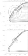 |
Fig. 2 Selected flow lines near the (B, V) plane for the cases with V = 2 km s−1, B = 7 µG, (model 5, upper panel), and V = 2 km s−1, B =20 µG, (model 17, lower panel). The two-stream structure of the stellar plasma flow (L and R streams) and the possible tail region (T) are indicated. The circles indicate the distances of 2 RTS, 4 RTS, and 6 RTS from the star, where RTS is the distance to the termination shock. |
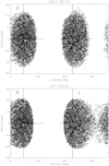 |
Fig. 3 Longitude-latitude distributions of the flow lines crossing points on the sphere with a radius of 300 AU and the centre at the host star for two cases with low inflow speed: V = 0.5 km s−1, nH,IS = 0.1 cm−3 (model 4, upper panel), V = 2km s−1, nH,IS =0.1 cm−3 (model 5, lower panel). B = 7 µG in all cases. Crossed lines show the direction and anti-direction of the interstellar field. |
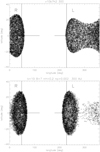 |
Fig. 4 As Fig. 3, but for the ISM inflow speed V = 10 km s−1. The upper panel (model 9) corresponds to the ISM proton density np,IS = 0.06 cm−3, and the lower panel (model 11) to a very low density np,IS = 0.002 cm−3. In both cases, B = 7 µG and nH,IS = 0.2 cm−3. |
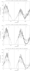 |
Fig. 5 Number of the flow lines that cross the spheres at a distance 3 RTS (solid line) and 2 RTS (dotted) from the star vs the astro-spheric longitude ϕ for three cases (in order from the top): V = 2 km s−1, B = 3 µG (model 1), V = 2 km s−1, B = 7 µG (model 5), and V = 5 km s−1, B = 20 µG (model 18). Boundaries of the R, L, and T sectors are marked by vertical dash-dotted lines. |
R, L, and T fluxes (total flux = 9999) at astrocentric distances 200–999 AU (models with V = 0.1, 0.5, 2, and 5 km s−1 ).
3.2 Closing of the astrotail
To observe the evolution of the astrospheric flow far downstream (i.e. in the direction of the ISM flow), it is convenient to consider the crossings of flow lines with the planes perpendicular to the x-axis, downstream from the host star. Instead of longitude-latitude plots of the crossing points, we used plots in the (y, z) plane. We then divided the y-axis into bins of equal length and added the numbers of crossings in each bin together. The results are shown in Figs. 8 (the B = 7 µG case) and 9 (the B = 20 µG case). The range of y was chosen to include all 9999 flow lines.
Figure 8 includes the cases of a very low relative speed between the ISM and the star: V = 0.1 km s−1 and V = 0.5 km s−1.
For these cases, there is a region without crossing points between the L and R peaks (the L peak lies in the negative y region). A possible interpretation is that the astrosphere has the tubelike topology. For the case V = 2 km s−1, there is a region with a low but non-zero number of crossings between the peaks. We conclude that for the case B = 7 µG, the closing of the astrotail occurs between V = 0.5 and V = 2 km s−1.
The case of B = 20 µG (Fig. 9) is included here not as a realistic example in the Galactic disk region, but for the purpose of comparison. In this case, a wide gap opens in the number of crossings between the L and R peaks for V = 2 km s−1. For V = 5 km s−1, there is a region with a very low number of crossings (much lower than for the V = 2 km s−1, B = 7 µG case), and for V = 15 km s−1, the flux in the region between the two peaks is only about 2 times lower than the L peak.
In these examples, the L peak is broader and lower than the R peak. The exception is the lowest value of V (0.1 kms−1 for B = 7 µG and 2 km s−1 for B = 20 µG). The closing of the astro-tail between V = 0.5 km s−1 and V = 2 km s−1 for B = 7 µG and between V = 2 km s−1 and V = 5 km s−1 for B = 20 µG agrees with our results for the shape of the astrosphere obtained by backward integration of flow lines (Figs. 13 and 14).
It is interesting that for the B = 7 µG and B = 20 µG cases (taking the same value of np,IS = 0.06 cm−3), the closing occurs within similar intervals of the Alfvénic Mach number MA for the interstellar plasma flow: for B = 7 µG MA = 0.008 at V = 0.5 km s−1 (tail closed) and MA = 0.032 at V = 2 km s−1 (tail open), and for B = 20 µG MA = 0.011 at V = 2 km s−1 (tail closed) and MA = 0.028 at V = 5 km s−1 (tail open). An order-of-magnitude estimation would place the tail crossing in the 0.01–0.03 interval of MA.
The question now is whether a tube-like astrosphere can appear when the inflow ISM speed is of the order of 10 km s−1. In Figs. 10 and 11, we plot the number of flow lines that cross the plane at x = 300 AU downstream from the star as a function of the coordinate y for different models with the same inflow speed V = 10 km s−1. For models with an ISM proton density np = 0.06 cm−3 as used in most of our simulations, we obtain a two-peak structure (Fig. 10, nH,IS = 0.5 cm−3), but with a weak contrast between the peak and the minimum value. The two-stream structure, however, becomes more pronounced when we assume a lower value of np,IS = 0.01 cm−3 (solid line in Fig. 10).
Figures 11 and 12 present the results obtained for nH,IS = 0.2 cm−3 for low proton densities: 0.002 cm−3 (B = 7 µG), 0.002 cm−3 (B =10 µG) and 0.015 cm−3 (B = 20 µG). The two streams are now much better separated, with the flux density in the link less than 10% of the peak values. Termination shocks and the astropauses in the (x, z) plane are shown in Fig. 15.
R, L, and T fluxes (total flux = 9999) at astrocentric distances of 200 to 999 AU (models with V = 10, 15 and 20 km s−1).
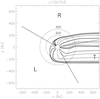 |
Fig. 6 Selected flow lines near the (B, V) plane for the case of high inflow speed and high neutral density (model 12: V = 10 km s−1, B = 7 µG, nH,IS =0.5 cm−3). The limits of the R, L, and T sectors are indicated by radial dotted straight lines. The circles show the limits of the regions within 200 and 300 AU from the star. The flow lines starting in the L sector cross into the T sector at the astrocentric distance ≤300 AU. |
3.3 Effect of the magnetic field of the host star
Because we considered only the time-stationary models, our simulations of the magnetic field of the host star are restricted to the case in which the stellar magnetic field is constant in time.
The boundary condition for the stellar magnetic field is defined at the inner boundary, which in most of our simulations is a sphere at 30 AU from the star. The rotation axis of the host star we assumed to be directed along the (astrospheric) latitude θ = 47° and longitude ϕ = 83°. This assumption introduces an asymmetry with respect to the (B, V) plane. For numerical reasons (to avoid numerical reconnection across the boundary between the regions of opposite polarity), we took the magnetic field not in the form of a dipole, but a monopole (Czechowski et al. 2010; see also the discussion in Pogorelov et al. 2017, 2021).
Let Θ and Φ denote the polar and azimuthal angles defined relative to the rotation axis of the host star. To obtain the boundary condition for the stellar magnetic field, we assumed that near the inner boundary, the magnetic field is given by the following analytical model (see Weber & Davis 1967):
 (1)
(1)
 (2)
(2)
 (3)
(3)
where Ω = 2π/Trot is the rotation rate of the star (we assumed Trot = 25.4 days), VSW = 750 km s−1 is the stellar wind speed (Table 1), and  is the value of Br at 1 AU from the star (0 or 37.5 Table 2). The conditions ∇ · B = 0 and ∇× (VSW × B) = 0 (the freezing condition) are satisfied by the model. The inner boundary conditions for the magnetic field are given by the values of the magnetic field components (Eqs. (1), (2), and (3)) calculated at the distance 30 AU from the star.
The effect of the stellar magnetic field on mass flow distribution is shown in Figs. 16, 17, and 18. Figure 16 shows the longitude-latitude plots of flow lines crossing points for the case V = 2 km s−1, B = 7 µG at distances of 300 AU (upper plot) and 500 AU (lower plot). Most of the L stream is shifted to negative latitudes.
Figures 17 and 18 show the numbers of flow lines crossing points versus astrospheric longitude at astrocentric distances of 3 RTS and 6 RTS, respectively. In each case, the upper panel shows the distribution of flow lines separately above (solid lines) and below (dotted lines) the (B, V) plane: the asymmetry is pronounced, most of the L stream flows below the plane. The middle panel shows the result of adding the two distributions together: the result can then be compared to the case without the stellar magnetic field, which is shown in the bottom panel. We conclude that the stellar magnetic field produces a large asymmetry in the distributions of flow lines relative to the (B, V) plane, but the effect on the two-stream structure of the flow is weak (compare models 4 and 4b in Table 4).
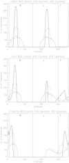 |
Fig. 7 Number of the flow lines that cross the spheres at a distance of 800 AU (solid line), 500 AU (dotted), and 300 AU (dashed line) from the star vs the astrospheric longitude ϕ for three cases (in order from the top): V = 0.5 km s−1, B = 7 µG (model 4), V = 2 km s−1, B = 7 µG (model 5), and V = 10 km s−1, B = 7 µG (model 9). For clarity, the data were averaged over 3° longitude bins. Boundaries of the R, L, and T sectors are marked by vertical dash-dotted lines. |
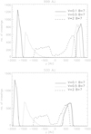 |
Fig. 8 Number of the flow lines that cross the planes x = 999 AU (upper panel), and x = 500 AU (lower panel) plotted vs. the coordinate y (see Fig. 1). Solid, dotted, and dashed lines correspond to the cases V = 0.1 km s−1 (model 3), V = 0.5 km s−1 (model 4), and V = 2 km s−1 (model 5), respectively. B = 7 µG for all cases. |
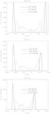 |
Fig. 9 Number of the flow lines that cross the planes x = 999 AU (upper panel), x = 500 AU (middle panel), and x = 200 AU (lower panel) plotted vs the coordinate y (see Fig. 1). Solid, dotted, and dashed lines correspond to the cases V = 2 km s−1 (model 17), V = 5 km s−1 (model 18), and V = 15 km s−1 (model 22), respectively. B = 20 µG, nH,IS = 0.1 cm−3 and np,IS = 0.06 cm−3 for all cases. |
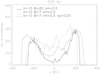 |
Fig. 10 Number of the flow lines that cross the plane x = 300 AU plotted vs the coordinate y (see Fig. 1) for an ISM neutral density nH,IS = 0.5 cm−3. The following cases are shown: V = 10 km s−1, B =20 µG, np,IS =0.06 cm−3 (model 21, solid line), V = 10 km s−1, B = 7 µG, np,IS =0.06cm−3 (model 12, dotted line), and V = 10 km s−1, B = 7 µG, np,IS =0.01 cm−3 (model 13, dashed line). |
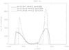 |
Fig. 11 Number of the flow lines that cross the plane x = 300 AU plotted vs the coordinate y (see Fig. 1) for an ISM neutral density nH,IS = 0.2 cm−3. The following cases are shown: V = 10 km s−1, B = 7 µG, np,IS = 0.002cm−3 (model 11, solid line), V = 10 km s−1, B =10 µG, np,IS = 0.004 cm−3 (model 16, dotted line), and V = 10 km s−1, B =20 µG, np,IS =0.015 cm−3 (model 20, dashed line). |
3.4 Very low density of neutral hydrogen in the ISM
Most of our simulations assumed a number density 0.1−0.5 cm−3 of the neutral hydrogen component in the ISM. We also performed simulations with a very low value (nH,IS = 0.001 cm−3) of this density. The effect of this change on the size of the astro-sphere is quite strong. In the (B, V) plane, the boundaries of the astrospheres approach the limit of our calculation domain.
Figure 19 shows selected flow lines near the (B, V) plane for two cases with the same value of the ISM inflow speed (2 km s−1), but two different values of the interstellar magnetic field strength (3 µG and 7 µG). In both cases, the R and L streams show no signs of turning downstream up to at least 5000 AU from the star. For B = 7 µG, the streams are well collimated, but for B = 3 µG, they spread out.
In Fig. 20, we show the numbers of flow lines that cross a sphere with a radius of 4000 AU plotted against the astrospheric longitude. For B = 7 µG, there are two narrow, well-separated peaks, but for B = 3 µG, the peaks are wider and linked by the tail.
Finally, Fig. 21 presents the distribution of the crossing points over the same sphere for B = 7 µG. There are some crossing points between the streams (too few to be visible in the upper plot of Fig. 20). If we take the limits of the stream regions in longitude to be 30–60 deg for R and 210–260 deg for the L stream, the number of crossing points outside is 40, that is, only 0.4% of the total flow. The question is whether a stable astrotail could be maintained by only 0.4% of the total plasma flow from the host star.
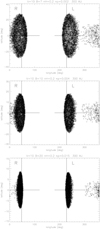 |
Fig. 12 Longitude-latitude distributions of the crossing points of the flow lines with the sphere of radius 300 AU for the cases illustrated in the Fig. 11. |
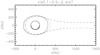 |
Fig. 13 Astropause and the termination shock in the “meridional” (x, z) plane for B = 7 µG assuming nH,IS = 0.1 cm−3 for V = 0.1 km s−1 (solid line, model 3) 0.5 km s−1 (dotted line, model 4) and 2 km s−1 (dashed line, model 5). |
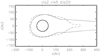 |
Fig. 14 As previous figure, but for B = 20 µG assuming V = 5 km s−1 (solid line, model 18) and 2 km s−1 (dashed line, model 17). |
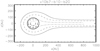 |
Fig. 15 As the previous figure, but for V = 10 km s−1 nH = 0.2 cm−3 assuming B = 7 µG, np,IS = 0.002 cm−3 (solid line, model 11), B = 10 µG np,IS = 0.004 cm−3 (dotted line, model 16), and B = 20 µG np,IS = 0.015 cm−3 (dashed line, model 20). |
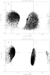 |
Fig. 16 Longitude-latitude distributions of the flow line crossing points on the spheres at 300 AU (top) and 500 AU (bottom) from the host star for the case V = 2 km s−1, B = 7 µG including the stellar magnetic field (model 6). The crossed lines show the direction and anti-direction of the interstellar field. |
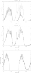 |
Fig. 17 Distribution in longitude of the number of the flow lines that cross the sphere at a distance of 3 RTS from the host star for the case V = 2 km s−1, B = 7 µG, including the magnetic field of the host star (model 6). In the upper panel, the solid (dotted) lines show the numbers of the crossing points above (below) the (B, V) plane. The middle panel shows the sum of both. The lower panel shows the result for the case in which the stellar magnetic field is neglected (model 5). |
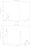 |
Fig. 18 As the previous figure, but for a distance of 6 RTS from the star (the middle panel is omitted). |
4 Discussion and conclusions
We have considered the distributions of stellar wind mass flux (approximated by a finite set of plasma flow lines) in a variety of model astrospheres based on simple MHD simulations. The parameters of the star and of the stellar wind, as well as the angle between the interstellar field and the ISM flow direction, were the same in all simulations and are close to the respective values that are commonly assumed for the Sun.
Our main result is that the two-stream structure of the plasma flow inside the astrosphere appears in most of our simulations. Downstream from the stellar wind termination shock, the flow is dominated by two streams (R and L streams), which initially are directed approximately along and opposite to the interstellar magnetic field. This structure arises because of anisotropic pressure of the interstellar magnetic field, as predicted by Parker (1961, 1963). The remaining part of the flow forms the tail component.
In some cases, the tail component is absent (the closed tail case) and the flow consists of two disjointed streams. The astropause then has the topology of a tube. The weak tail occurs when the tail component is only a very small fraction of the total plasma flow.
If the interstellar medium includes a non-negligible neutral component, the directions of the streams are affected by chargeexchange between the astrospheric plasma and the neutral ISM. At large distances from the star, the astrospheric flow becomes then parallel to the flow direction of the undisturbed ISM. If the neutral ISM density is high (0.5 cm−3 for B = 7 µG and a solar-type host star), the astrosphere contracts and no two-stream structure develops (see Fig. 6).
Simulations that include the stellar magnetic field lead to astrospheres that are not symmetric with respect to the (B, V) plane. The conclusion about the domination of two streams is still valid, but with the L stream moving below the (B, V) plane.
We used four values of the interstellar magnetic field strength (B = 3, 7, 10, and 20 µG) and seven values of the ISM speed relative to the host star (0.1, 0.5, 2, 5, 10, 15, and 20 km s−1). The ISM plasma density was set to 0.06 cm−3 in most cases. The neutral density values were 0.1 cm−3, 0.2cm−3, or 0.5 cm−3. We also considered some examples with a very low interstellar neutral density (nH,IS = 0.001 cm−3) or a very low interstellar proton density (between 0.002 cm−3 and 0.015 cm−3). In most calculations, the stellar magnetic field was ignored: when it was included, we assumed a monopole orientation.
We found a closing of the astrotail only for a very low ISM inflow speed: 0.1 and 0.5 km s−1 if B = 7 µG and 2 km s−1 for the extreme case of B = 20 µG. For both B = 7 µG and B = 20 µG, the closing occurs for similar ranges of the Alfvénic Mach number of the interstellar flow. For V = 5 km s−1, B = 20 µG, the flow in the tail region was not zero, but very weak. A weak tail flow was also found for V = 2 km s−1, B = 7 µG with a very low IS neutral density. All these results were obtained by time-stationary calculations. To answer the question of stability of the astrotail in the weak tail case, we must consider time-dependent models.
For a higher inflow speed (V = 10 km s−1), we found that although no tube-like topology was reached, the flow structure may be very close to it provided that proton density in the ISM is very low. The tail component becomes less than 10% of the peak flux for an ISM proton density of 0.015 cm−3 for B = 20 µG, 0.004 cm−3 at 10 µG, and 0.002 cm−3 at 7 µG. The ISM neutral density was 0.2 cm−3 in these cases. Our results imply that tubelike astrospheres occupy only a small region of the parameter space.
A question of interest is whether the astrospheres discussed in this work might be observed. Leaving aside the case of hot stars, most detections of astrospheres are based on observations of the Ly α line in the spectrum of the host star. The signature of an astrosphere is the absorption of the Ly α line (additional to absorption by the ISM) by the hydrogen wall (Zank et al. 2013), which forms by a slowing-down of the ISM in front of the astrosphere.
This method of observation becomes inefficient for the astrospheres we considered. For a slow inflow speed and also for a weakly ionised ISM, the hydrogen wall would be a weakly developed structure and the astrospheric absorption would be difficult to detect. In any case, the observation would not provide any details about the structure of the flow inside the astrosphere.
Astrospheric absorption might also be observed in the absence of a hydrogen wall. For the case of the heliosphere, Ly α absorption was detected in the heliotail direction (Wood et al. 2014). A feature of the two-stream astrosphere that might be observed in principle are fast collimated plasma streams. The fast-flowing plasma in the stream can accelerate the neutral atoms from the ISM by charge-exchange. An observer looking upstream could then attempt to detect the shifted absorption of the Ly α line from the star by the accelerated neutral atoms. For a solar-type star as assumed in our simulations, this effect would, however, be much weaker than the Ly α absorption by the hydrogen wall observed in the usual astrospheres: the estimation using a simple model of the flow implies that only a few percent of neutral H would be accelerated.
A desirable technique of observation would be one that permits imaging of the astrospheric structure. Baalmann et al. (2020) investigated the possibilities of observing the astrospheres by measuring different observables, in particular, H α emission. The astrospheres were described by four MHD models, including the solar heliosphere (observer at a distance of 1 pc) and the astrosphere of λ Cephei (observer at 617 pc). Only for λ Cephei was the Ha flux above the current observational threshold. The bow shock was the only feature that could be distinguished.
Finally, we comment on the relation between the two-stream structure and the heliosphere. The results of our simulations together with the estimated parameters of the local ISM (V~26 km s−1, B ~ 3µG: Zirnstein et al. 2016) do not suggest a two-stream structure for the heliosphere. A topology with a significant tube-like component has nevertheless been considered for the heliospheric plasma flow in connection with observations of the energetic neutral atoms by INCA and IBEX (Krimigis et al. 2009; McComas et al. 2013). A possible explanation of the departure from the expected comet-like structure of the heliosphere is provided by a class of models of the astrospheres with a tube-like structure, for which the flow inside the astrosphere is shaped not by the interstellar magnetic field, but by the magnetic field of the host star (Golikov et al. 2017; Korolkov & Izmodenov 2021). A related mechanism that was first described theoretically by Yu (1974) leads to a splitting of the plasma flow (the split-tail structure) in some models of the heliosphere (Opher et al. 2015, Pogorelov et al. 2021). According to Pogorelov et al. (2021), the split flow merges into a single heliotail when realistic boundary conditions are used.
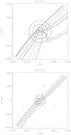 |
Fig. 19 Selected flow lines near the (B, V) plane for the astrospheres with V = 2 km s−1, B = 3 µG (model 2, upper plot) and V = 2 km s−1, B = 7 µG for the case of very low density of the neutral component of the ISM (nH,IS = 0.001 cm−3, model 7, lower plot). The outlines of the spheres at 2 RTS, 4 RTS, and 6 RTS are also shown. |
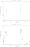 |
Fig. 20 Number of flow lines that cross the sphere at 4000 AU from the star vs astrospheric longitude. Two cases are illustrated: B = 7 µG (upper panel, model 7) and B = 3 µG (lower panel, model 2). The values of V (2 km s−1) and nH,IS (0.001 cm−3) are the same for both cases. |
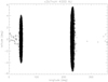 |
Fig. 21 Longitude-latitude distribution of the flow lines crossing points on a sphere with a radius of 4000 AU and the centre at the host star for the case V = 2 km s−1, B = 7 µG, nH,IS = 0.001 cm−3 (model 7). In addition to the R and L streams, there are a few crossing points in the tail region (less than 1% of the total flux). |
Acknowledgements
We thank the referee (Will Henney) for helpful comments.
References
- Baalmann, L. R., Scherer, K., Fichtner, H., et al. 2020, A&Amp;A, 634, A67 [NASA ADS] [CrossRef] [EDP Sciences] [Google Scholar]
- Belfort, P., & Crovisier, J., 1984, A&Amp;A, 136, 368B [NASA ADS] [Google Scholar]
- Czechowski, A., Strumik, M., & Grygorczuk, J. 2010, A&Amp;A, 516, A17 [NASA ADS] [CrossRef] [EDP Sciences] [Google Scholar]
- Czechowski, A., & Grygorczuk, J. 2017, J. Phys.: Conf. Ser., 900, 012004 [NASA ADS] [CrossRef] [Google Scholar]
- Decin, L., Cox, N. L. J., Royer, P., et al. 2012, A&Amp;A, 548, A113 [NASA ADS] [CrossRef] [EDP Sciences] [Google Scholar]
- Golikov, E. A., Izmodenov, V., Alexashov, D. B., & Belov, N.A. 2017, MNRAS, 464, 1065 [CrossRef] [Google Scholar]
- Korolkov, S., & Izmodenov, V. 2021, MNRAS, 504, 4589 [NASA ADS] [CrossRef] [Google Scholar]
- Krimigis, S. M., Mitchell, D. G., Roelof, E. C., Hsieh, K. C., & McComas, D. J. 2009, Science, 326, 971 [NASA ADS] [CrossRef] [Google Scholar]
- Linsky, J. L., & Wood, B. E. 2014, ASTRA Proc., 1, 43 [NASA ADS] [CrossRef] [Google Scholar]
- Mackey, J., Green, S., & Moutzouri, M. 2020, J. Phys.: Conf. Ser., 1620, 012012 [NASA ADS] [CrossRef] [Google Scholar]
- Marchal, A., & Miville-Deschenes, M.-A. 2021, ApJ, 908, 186M [NASA ADS] [CrossRef] [Google Scholar]
- McComas, D. J., Dayeh, M. A., Funsten, H. O., Livadiotis, G., & Schwadron, N. A. 2013, ApJ, 771, 77 [NASA ADS] [CrossRef] [Google Scholar]
- Meyer, D. M.-A., Mackey, J., Langer, N., et al. 2014, MNRAS, 444, 2754 [NASA ADS] [CrossRef] [Google Scholar]
- Mueller, H., & Juric, A. 2021, Bull. Am. Astron. Soc., 53, 2021n1i553p04 [Google Scholar]
- Opher, M., Drake, J. F., Zieger, B., & Gombosi, T. I. 2015, ApJ, 800, L28 [NASA ADS] [CrossRef] [Google Scholar]
- Parker, E.N. 1961, ApJ, 134, 20 [NASA ADS] [CrossRef] [Google Scholar]
- Parker, E. N. 1963, Interplanetary Dynamical Processes (New York: Interscience) Pogorelov, N. V., Borovikov, S. N., Heerikhuisen, J., & Zhang, M. 2015, ApJ, 812, L6 [Google Scholar]
- Pogorelov, N. V., Heerikhuisen, J., Roytershteyn, V., et al. 2017, ApJ, 845, 9 [NASA ADS] [CrossRef] [Google Scholar]
- Pogorelov, N. V., Fraternale, F., Kim, T. K., Burlaga, L.F., & Gurnett, D. A. 2021, ApJ, 917, L20 [NASA ADS] [CrossRef] [Google Scholar]
- Ratkiewicz, R., Molvik, G. A., Spreiter, J. R., et al. 1998, A&Amp;A, 335, 363 [NASA ADS] [Google Scholar]
- Ratkiewicz, R., Barnes, A., Müller, H.-R., Zank, G. P., & Webb, G. M. 2002, Adv. Space Res., 29, 433 [NASA ADS] [CrossRef] [Google Scholar]
- Sahai, R., & Chronopoulos, C. K. 2010 ApJ, 711, L53 [NASA ADS] [CrossRef] [Google Scholar]
- Scherer, K., Fichtner, H., Kleimann, J., et al. 2016, A&Amp;A, 586, A111 [NASA ADS] [CrossRef] [EDP Sciences] [Google Scholar]
- Scherer, K., Baalmann, L. R., Fichtner, H., et al. 2020, MNRAS, 493, 4172 [Google Scholar]
- Struminsky, A., & Sadovski, A. 2019, J. Phys.: Conf. Ser., 1181, 012002 [NASA ADS] [CrossRef] [Google Scholar]
- Swaczyna, P., McComas, D. J., Zirnstein, E. J., et al. 2020, ApJ, 903, 48 [NASA ADS] [CrossRef] [Google Scholar]
- Swaczyna, P., Kubiak, M. A., Bzowski, M., et al. 2022, ApJS, 259, 42 [NASA ADS] [CrossRef] [Google Scholar]
- Van Marle, A. J., Meliani, Z., & Marcowith, A. 2015, A&Amp;A, 584, A49 [NASA ADS] [CrossRef] [EDP Sciences] [Google Scholar]
- Weber, E. J., & Davis, L. 1967, ApJ, 148, 217 [Google Scholar]
- Wood, B. E. 2004, Living Rev. Solar Phys., 1, 2 [NASA ADS] [CrossRef] [Google Scholar]
- Wood, B. E., Izmodenov, V. V., Alexashov, D. B., Redfield, S., & Edelman, E. 2014, ApJ, 780, 108 [Google Scholar]
- Wood, B. E., Müller, H.-R., & Harper, G. M. 2016, ApJ, 829, 74 [NASA ADS] [CrossRef] [Google Scholar]
- Yu, G. 1974, ApJ, 194, 187 [NASA ADS] [CrossRef] [Google Scholar]
- Zank, G. P., Heerikhuisen, J., Wood, B. E., et al. 2013, ApJ, 763, 20 [NASA ADS] [CrossRef] [Google Scholar]
- Zirnstein, E. J., Heerikhuisen, J., Funsten, H. O., et al. 2016, ApJ, 818, L18 [CrossRef] [Google Scholar]
All Tables
R, L, and T fluxes (total flux = 9999) at astrocentric distances 200–999 AU (models with V = 0.1, 0.5, 2, and 5 km s−1 ).
R, L, and T fluxes (total flux = 9999) at astrocentric distances of 200 to 999 AU (models with V = 10, 15 and 20 km s−1).
All Figures
|
Fig. 1 Definition of our coordinate system. The termination shock and the astropause in the (B, V) plane (model 1: V = 2 km s−1, B = 3 µG case) are outlined. The x- and y-axes lie on the (B, V) plane. The x-axis is directed along the ISM inflow. The z-axis (not shown) completes the right-handed system. The angle ϕ (the astrospheric longitude) is counted from the x-axis. The astrospheric latitude θ is counted from the (B, V) plane. Dash-dotted lines show the limits in longitude of the R, L, and T sectors. |
| In the text | |
|
Fig. 2 Selected flow lines near the (B, V) plane for the cases with V = 2 km s−1, B = 7 µG, (model 5, upper panel), and V = 2 km s−1, B =20 µG, (model 17, lower panel). The two-stream structure of the stellar plasma flow (L and R streams) and the possible tail region (T) are indicated. The circles indicate the distances of 2 RTS, 4 RTS, and 6 RTS from the star, where RTS is the distance to the termination shock. |
| In the text | |
|
Fig. 3 Longitude-latitude distributions of the flow lines crossing points on the sphere with a radius of 300 AU and the centre at the host star for two cases with low inflow speed: V = 0.5 km s−1, nH,IS = 0.1 cm−3 (model 4, upper panel), V = 2km s−1, nH,IS =0.1 cm−3 (model 5, lower panel). B = 7 µG in all cases. Crossed lines show the direction and anti-direction of the interstellar field. |
| In the text | |
|
Fig. 4 As Fig. 3, but for the ISM inflow speed V = 10 km s−1. The upper panel (model 9) corresponds to the ISM proton density np,IS = 0.06 cm−3, and the lower panel (model 11) to a very low density np,IS = 0.002 cm−3. In both cases, B = 7 µG and nH,IS = 0.2 cm−3. |
| In the text | |
|
Fig. 5 Number of the flow lines that cross the spheres at a distance 3 RTS (solid line) and 2 RTS (dotted) from the star vs the astro-spheric longitude ϕ for three cases (in order from the top): V = 2 km s−1, B = 3 µG (model 1), V = 2 km s−1, B = 7 µG (model 5), and V = 5 km s−1, B = 20 µG (model 18). Boundaries of the R, L, and T sectors are marked by vertical dash-dotted lines. |
| In the text | |
|
Fig. 6 Selected flow lines near the (B, V) plane for the case of high inflow speed and high neutral density (model 12: V = 10 km s−1, B = 7 µG, nH,IS =0.5 cm−3). The limits of the R, L, and T sectors are indicated by radial dotted straight lines. The circles show the limits of the regions within 200 and 300 AU from the star. The flow lines starting in the L sector cross into the T sector at the astrocentric distance ≤300 AU. |
| In the text | |
|
Fig. 7 Number of the flow lines that cross the spheres at a distance of 800 AU (solid line), 500 AU (dotted), and 300 AU (dashed line) from the star vs the astrospheric longitude ϕ for three cases (in order from the top): V = 0.5 km s−1, B = 7 µG (model 4), V = 2 km s−1, B = 7 µG (model 5), and V = 10 km s−1, B = 7 µG (model 9). For clarity, the data were averaged over 3° longitude bins. Boundaries of the R, L, and T sectors are marked by vertical dash-dotted lines. |
| In the text | |
|
Fig. 8 Number of the flow lines that cross the planes x = 999 AU (upper panel), and x = 500 AU (lower panel) plotted vs. the coordinate y (see Fig. 1). Solid, dotted, and dashed lines correspond to the cases V = 0.1 km s−1 (model 3), V = 0.5 km s−1 (model 4), and V = 2 km s−1 (model 5), respectively. B = 7 µG for all cases. |
| In the text | |
|
Fig. 9 Number of the flow lines that cross the planes x = 999 AU (upper panel), x = 500 AU (middle panel), and x = 200 AU (lower panel) plotted vs the coordinate y (see Fig. 1). Solid, dotted, and dashed lines correspond to the cases V = 2 km s−1 (model 17), V = 5 km s−1 (model 18), and V = 15 km s−1 (model 22), respectively. B = 20 µG, nH,IS = 0.1 cm−3 and np,IS = 0.06 cm−3 for all cases. |
| In the text | |
|
Fig. 10 Number of the flow lines that cross the plane x = 300 AU plotted vs the coordinate y (see Fig. 1) for an ISM neutral density nH,IS = 0.5 cm−3. The following cases are shown: V = 10 km s−1, B =20 µG, np,IS =0.06 cm−3 (model 21, solid line), V = 10 km s−1, B = 7 µG, np,IS =0.06cm−3 (model 12, dotted line), and V = 10 km s−1, B = 7 µG, np,IS =0.01 cm−3 (model 13, dashed line). |
| In the text | |
|
Fig. 11 Number of the flow lines that cross the plane x = 300 AU plotted vs the coordinate y (see Fig. 1) for an ISM neutral density nH,IS = 0.2 cm−3. The following cases are shown: V = 10 km s−1, B = 7 µG, np,IS = 0.002cm−3 (model 11, solid line), V = 10 km s−1, B =10 µG, np,IS = 0.004 cm−3 (model 16, dotted line), and V = 10 km s−1, B =20 µG, np,IS =0.015 cm−3 (model 20, dashed line). |
| In the text | |
|
Fig. 12 Longitude-latitude distributions of the crossing points of the flow lines with the sphere of radius 300 AU for the cases illustrated in the Fig. 11. |
| In the text | |
|
Fig. 13 Astropause and the termination shock in the “meridional” (x, z) plane for B = 7 µG assuming nH,IS = 0.1 cm−3 for V = 0.1 km s−1 (solid line, model 3) 0.5 km s−1 (dotted line, model 4) and 2 km s−1 (dashed line, model 5). |
| In the text | |
|
Fig. 14 As previous figure, but for B = 20 µG assuming V = 5 km s−1 (solid line, model 18) and 2 km s−1 (dashed line, model 17). |
| In the text | |
|
Fig. 15 As the previous figure, but for V = 10 km s−1 nH = 0.2 cm−3 assuming B = 7 µG, np,IS = 0.002 cm−3 (solid line, model 11), B = 10 µG np,IS = 0.004 cm−3 (dotted line, model 16), and B = 20 µG np,IS = 0.015 cm−3 (dashed line, model 20). |
| In the text | |
|
Fig. 16 Longitude-latitude distributions of the flow line crossing points on the spheres at 300 AU (top) and 500 AU (bottom) from the host star for the case V = 2 km s−1, B = 7 µG including the stellar magnetic field (model 6). The crossed lines show the direction and anti-direction of the interstellar field. |
| In the text | |
|
Fig. 17 Distribution in longitude of the number of the flow lines that cross the sphere at a distance of 3 RTS from the host star for the case V = 2 km s−1, B = 7 µG, including the magnetic field of the host star (model 6). In the upper panel, the solid (dotted) lines show the numbers of the crossing points above (below) the (B, V) plane. The middle panel shows the sum of both. The lower panel shows the result for the case in which the stellar magnetic field is neglected (model 5). |
| In the text | |
|
Fig. 18 As the previous figure, but for a distance of 6 RTS from the star (the middle panel is omitted). |
| In the text | |
|
Fig. 19 Selected flow lines near the (B, V) plane for the astrospheres with V = 2 km s−1, B = 3 µG (model 2, upper plot) and V = 2 km s−1, B = 7 µG for the case of very low density of the neutral component of the ISM (nH,IS = 0.001 cm−3, model 7, lower plot). The outlines of the spheres at 2 RTS, 4 RTS, and 6 RTS are also shown. |
| In the text | |
|
Fig. 20 Number of flow lines that cross the sphere at 4000 AU from the star vs astrospheric longitude. Two cases are illustrated: B = 7 µG (upper panel, model 7) and B = 3 µG (lower panel, model 2). The values of V (2 km s−1) and nH,IS (0.001 cm−3) are the same for both cases. |
| In the text | |
|
Fig. 21 Longitude-latitude distribution of the flow lines crossing points on a sphere with a radius of 4000 AU and the centre at the host star for the case V = 2 km s−1, B = 7 µG, nH,IS = 0.001 cm−3 (model 7). In addition to the R and L streams, there are a few crossing points in the tail region (less than 1% of the total flux). |
| In the text | |
Current usage metrics show cumulative count of Article Views (full-text article views including HTML views, PDF and ePub downloads, according to the available data) and Abstracts Views on Vision4Press platform.
Data correspond to usage on the plateform after 2015. The current usage metrics is available 48-96 hours after online publication and is updated daily on week days.
Initial download of the metrics may take a while.