| Issue |
A&A
Volume 666, October 2022
|
|
|---|---|---|
| Article Number | A93 | |
| Number of page(s) | 14 | |
| Section | Astronomical instrumentation | |
| DOI | https://doi.org/10.1051/0004-6361/202142920 | |
| Published online | 13 October 2022 | |
Calibration scheme for space-borne full-disk vector magnetograph under the influence of orbiter velocity
1
Key Laboratory of Solar Activity, National Astronomical Observatories, Chinese Academy of Sciences,
Beijing
100101, PR China
e-mail: hzy@nao.cas.cn; chenjie@bao.ac.cn
2
Yunnan Observatories, Chinese Academy of Sciences,
Kunming
650216, PR China
e-mail: jkf@ynao.ac.cn
3
School of Astronomy and Space Science, University of Chinese Academy of Sciences,
Beijing
101408, PR China
4
College of Information and Computer, Taiyuan University of Technology,
Taiyuan
030024, PR China
5
Astrophysics Research Centre, School of Mathematics and Physics, Queen’s University,
Belfast
BT7 1NN, UK
6
Swedish Institute of Space Physics,
Scheelevagen 17,
223 70
Lund, Sweden
Received:
15
December
2021
Accepted:
30
May
2022
Context. The Full-disk Vector MagnetoGraph (FMG) is one of the three payloads on the Advanced Space-based Solar Observatory (ASO-S). The FMG is set to observe the full disk vector magnetic field at a single wavelength point. The magnetograph in orbit will encounter the wavelength shift problem caused by the Doppler effect in the magnetic field, which mainly comes from the Sun’s rotation velocity and the satellite–sun relative velocity.
Aims. We look to use neural networks for single-wavelength calibration to solve the wavelength shift problem.
Methods. We used the existing data from the Helioseismic and Magnetic Imager (HMI) on the Solar Dynamics Observatory (SDO). To simulate plausible single-wavelength observations, we used the Stokes polarization image from the HMI at a single wavelength point. We also input the satellite orbital velocity given by the HMI data file and the solar rotation velocity to the network. We developed a set of data preprocessing methods before entering the network and we trained the network to get the calibration model.
Results. By analyzing and comparing the prediction of the neural network with the target magnetogram, we believe that our network model has learned a single-wavelength full-disk calibration model. The mean absolute error (MAE) of the longitudinal field and the transverse field of the full disk are 3.68 G and 28.08 G, respectively. The MAE error of the azimuth angle of pixels above 300 G is 12.29°.
Key words: magnetic fields / Sun: magnetic fields
© Z. Hu et al. 2022
 Open Access article, published by EDP Sciences, under the terms of the Creative Commons Attribution License (https://creativecommons.org/licenses/by/4.0), which permits unrestricted use, distribution, and reproduction in any medium, provided the original work is properly cited.
This article is published in open access under the Subscribe-to-Open model. Subscribe to A&A to support open access publication.
1 Introduction
Astronomers had begun to measure the solar magnetic field by observing the Zeeman effect of sunlight (Hale 1908). The measurement of the solar magnetic field is mainly based on observing the polarization of sunlight. For spectroscopic magnetic imagers observed at multiple wavelength points, the vector magnetic field can be obtained through an inversion of the Stokes profile of the spectrum (Skumanich & Lites 1987; Ruiz Cobo & del Toro Iniesta 1992; Socas-Navarro 2001; Asensio Ramos & de la Cruz Rodríguez 2015; Li et al. 2019). One such device in operation is the Stokes Spectro-Polarimeter (SP) on the Hinode satellite (Tsuneta et al. 2008). For filter-type magnetic imagers observing at a single wavelength point or limited wavelength points, a linear calibration method is used (Bai et al. 2013, 2014; Ai et al. 1982). There are also some filter-type magnetic imagers observed at multiple wavelength points, such as the Helioseismic and Magnetic Imager (HMI) on the Solar Dynamics Observatory (SDO) (Schou et al. 2012; Pesnell et al. 2012). Linear calibration is based on the assumption of a weak field approximation (Stenflo 1994). When the magnetic field is weak enough or the Lande factor of the spectral line is small enough, the vector magnetic field parameter can be expressed as a linear function of the Stokes parameters (Jefferies et al. 1989):
 (1)
(1)
 (2)
(2)
 (3)
(3)
Here, Cl and Ct are calibration coefficients that are to be determined, however, in strong magnetic fields, the linear calibration method eventually encounters the problem of magnetic saturation. In regions with a weak magnetic field, the polarization signal becomes stronger as the magnetic field increases. In strong field regions, however, the polarization signal becomes weaker as the magnetic field becomes larger because the Zeeman split distance increases. The linear calibration must then face the influence of the magneto-optical effect in the measurement of the azimuth angle, resulting in larger errors in the strong field area (Hagyard et al. 2000; Su & Zhang 2004).
The Advanced Space-based Solar Observatory (ASO-S) (Gan et al. 2019) is expected to be launched in 2022 in order to observe the maximum of the Solar Cycle 25. Full-disk Vector MagnetoGгaph (FMG) is one of the three payloads of ASO-S (Deng et al. 2019). The purpose of FMG is to detect the vector magnetic field of the entire disk with high time and spatial resolution. As a filter-based magnetograph that mainly works in single-wavelength observation mode, FMG currently plans to acquire magnetic field images with linear calibration (Su et al. 2019). As a satellite-borne full-disk magnetograph, FMG is subject to wavelength shifts caused by two important Doppler velocities during the calibration process. One is the relative movement velocity between the satellite and the sun caused by the orbital velocity of the satellite. The other is the relative movement velocity of the solar surface relative to the satellite caused by the solar rotation. In addition, HMI is also a space-based full-disk magnetic imager. It is estimated that the line-of-sight solar-satellite velocity brought by the orbital velocity is in the range of ±3.5 km s−1 and the line-of-sight component of the sun’s rotation velocity is in the range of ±2 km s−1 (Centeno et al. 2014).
Due to the movement of the center of the spectral line, the image I(λ) taken by the detector at the wavelength λ is actually the signal I(λ + Δλ) sent by the sun at λ + Δλ. Depending on whether this movement makes the observation point closer to or far from the center of the line, I(λ + Δλ) will be greater or less than I(λ). If a magnetograph is observing at enough wavelength points, for example Hinode/SP at 112 points, then even if the spectral line moves, we can still get a good enough fit to get the true spectral line profile. But when the observed wavelength points are relatively few, it is obvious that the fitting of the spectral line profile will be distorted due to wavelength shift. In the extreme case, for a magnetic imager that observes at a single wavelength point, if the Doppler velocity information is not considered, it is difficult to judge whether the signal change is the real signal change or whether it is caused by the Doppler velocity. Therefore, the linear calibration will end up with a large error in this case.
We consider that the line-of-sight components of the orbital velocity and the rotation velocity are known. In the magnetic field calibration mission, the orbital velocity is given by the satellite operation information. The rotation velocity can be calculated from the formula of the solar rotation to get a theoretical value. Therefore, we want to find a method that can use the velocity information to correct the vector magnetic field calibration. The calibration of the magnetic field is actually to find the functional relationship between the Stokes signal of a single or multiple wavelength points to the vector magnetic field parameters. Therefore, the single-wavelength calibration affected by the Doppler velocity is to determine a function relationship from a set of Stokes parameters and the corresponding Doppler velocity information to the vector magnetic field parameters. This is exactly the fitting task that artificial neural networks (ANNs) are optimized for. Currently, ANNs serve as a mature machine learning methods used in a variety of regression and classification tasks. Hornik (1991) has pointed out the powerful representation ability of ANN for nonlinear functions, which is the so-called universal approximation theorem. It has been used in many astronomical fields, such as solar magnetic field calibration. At the earliest, Carroll & Staude (2001) used a multi-layer perceptron (MLP) to fit the Stokes inversion of 81 wavelength points to output many parameters such as total magnetic field. Socas-Navarro (2003) developed an inversion method based on principal component analysis (PCA). They also used PCA for the preprocessing of neural network input data and reduced the dimensionality of the data to accelerate network prediction (see Socas-Navarro 2003). Carroll et al. (2008) used MLP to model the radiative transfer of Zeeman-Doppler imaging and Stokes profile inversion. Teng (2015) used statistical machine learning techniques based on the Mercer kernel to invert the photosphere’s magnetic field from polarization data. Asensio Ramos & Díaz Baso (2019) applies convolutional neural network (CNN) to solar magnetic field calibration for the first time. Guo et al. (2020, 2021) used MLP and CNN to perform magnetic field inversion on Hinode/SP data and demonstrated the feasibility of neural network for single-wavelength magnetic field calibration. Higgins et al. (2021) used the unet code to invert the HMI/SDO data and used the output of regression-by-classification. Bai et al. (2021) suggested a new method for quickly estimating the unsigned radial component of the magnetic field and the transverse field by CNN solely on the basis of photospheric continuum images.
Our work is aimed at applying CNN to calibrate single-wavelength vector magnetic field affected by two Doppler velocities. We use existing multi-wavelength space-borne observation data to simulate this scenario. We introduce the data set and the preprocessing process before the data enters the network in Sect. 2. In Sect. 3, the established network model, the loss function used, and the training are described. We show the results of the network output in Sect. 4 and we discuss the quality of the network output in Sect. 5.
2 Dataset and data preprocessing
2.1 Dataset
We used the data from SDO/HMI to simulate the future observation of ASO-S/FMG. Observations by HMI cover polarization images at six wavelength points near the Fe I 6173.34 Å spectral line (Norton et al. 2006; Schou et al. 2012). Then the Very Fast Inversion of the Stokes Vector code (VFISV) (Borrero et al. 2011) inverts the Stokes profile to obtain the vector magnetic field image and other solar atmospheric parameters. In this study, data is selected from HMI 720s data product series (Hoeksema et al. 2014). The HMI instrument generates a group of images with 4096 × 4096 pixels every 720 s. There are Stokes parameters (I, Q, U, and V) at six wavelengths in level 1 data (hmi.S_720s) and vector magnetic field in level 2 data (hmi.B_720s). We chose the data of the second wavelength point. This is probably the half-peak position of the I signal without wavelength shift. We separate the obtained data into training set, validation set, and test set. The data before 2015 is used as the training and validation set and the data from 2015 and later is used as the test set. During training, due to the limitation of the video memory size of the GPU, it is impossible to load the image with 4096 × 4096 pixels and network for back propagation and parameter update. Therefore, we cut the image into a small size around the active regions and loaded it with a big batch-size in training. In our experiments, this small size is 256 × 256 pixels. The benefit of cropping is to balance the data set, which we will discuss later in the neural network training method. In order to quickly iterate to correct the hyperparameters, we also want a validation set of small-sized images. Therefore, the full disk data of the training and validation set are cut into small-size images before they are randomly divided into 8:2.
2.2 Preprocessing
To calibrate the full-disk magnetic field in the presence of the wavelength shift, the data preprocessing in this study is important. This operation can remove as much as possible the influence of different positions on the solar surface and the different relative velocities between the satellite and the sun.
The most important part of the preprocessing is the processing of the I channel. The processing of I consists of two steps, dealing with limb darkening and dealing with what we call tilt. In Fig. 1, we show the original I and the I after different processing steps. This is equivalent to looking at the entire disk from the side of the 2D solar image and we can see that the signal intensity is unevenly distributed on the disk. In the original I, the low curve is mostly a straight line, which comes from the edge of the Sun. Because of the edge-dimming effect, the edge part of the disk is obviously darker than the middle part. This effect can be coarsely seen from the shape of the median and high curves. Parts of the low curve with significantly low value come from sunspots.
The way we deal with limb darkening is to calculate the limb darkening image and use it to divide the I image. Limb darkening can be expressed as follows, where θ is the heliocentric angle:
 (4)
(4)
where Iλ(0, 0) is the radiation intensity at the center of the solar surface. It can be assumed that Fλ is the second-order form of
 (5)
(5)
We used the least-squares method to fit Eq. (5) to the original I image. It should be noted that the right formula is only a ratio, which is a dimensionless quantity. However, the direct result of fitting the image is actually Iλ(0, θ), which is equal to the right formula multiplied by Iλ(0, 0). For a single image, Iλ(0, 0) is a constant, namely, the signal strength at the center of the Sun. We divide the original image by the limb darkening obtained by fitting to get an image with the limb darkening removed. Since the Iλ(0, θ) obtained by fitting has the same order of magnitude and the same unit as the original image, this operation also normalizes the image. Therefore, the processed image is dimensionless and the order of magnitude is 1. When fitting, a threshold used is the median of the low curve. This setting assumes that the sunspot area occupies a small area on the sun, so the median value of the low curve comes from the edge area of the solar surface. The fitting of limb darkening only uses pixels above the threshold. This is meant to avoid the influence of pixels in the sunspot area. Fig. 2 is a 2D image of limb darkening obtained by fitting. We divide the original image by Fig. 2 to get the image with the limb darkening background removed. It can be seen in the middle panel of Fig. 1 that the image after dealing with the limb darkening has been normalized. The vast majority of pixels are between 0 and 1, and a small number of pixels exceed 1.
It is worth noting that the curves in the middle panel of Fig. 1 are tilted. The entire disk appears dark on one side and bright on the other. One of the reasons for this tilt is the wavelength shift caused by the solar rotation. Like limb darkening, the uneven background of this signal intensity distribution should be removed. According to the image, we assume that this tilt background is linear with respect to pixel coordinates. The method for removing this tilt background still involves using the least-squares method to fit it, followed by the use of the fitted 2D image to remove the image obtained in the previous step.
When single-wavelength images taken at the same wavelength position are calibrated under different wavelength shifts, it is equivalent to having different calibration functions. Thus, we hope to let the network learn the calibration relationship in different situations by inputting the wavelength shift information. Because the wavelength shift is caused by the velocity of relative motion, it is reasonable to believe that the velocity infor-matio n can be used to indicate different wavelength shifts. There are two main sources of velocity in magnetic field measurement: the line-of-sight velocity between the Sun and the spacecraft and the Sun rotation velocity. The range of these two velocities can be assumed to be ±3.5 km s−1 and ±2kms−1 (Centeno et al. 2014). The line-of-sight velocity between th e sun and the s pacecraft is given in the header of trie HMI data file, which is the OBSVR keyword, and OBSVR takes the positive sign when the satellite is far away from the Sun. In the following, we use OBSVR to represent the line-of-sight velocity between the sun and the spacecraft, and use a similar method to represent other velocity terms. For a measurement at a certain moment, OBSVR is scalar. In order to enter the network together with the polarizaaion parameter, we expand it into a 2D array witti all the same values as the OBSVR channel in the input data.
The rotation velocity of the Sun input to the network is a theoretical value obtained from
 (6)
(6)
where ϕ is the latitude. The parameters used are from Timothy et al. (1975)). We multiply the angular velocity by the radius of the latitude circle to obtain the rotation linear velocity of different pixels. Due to the Doppler effect caused by velocity, the line-of-sight component of velocity is important. We project the rotation velocity to the sun-spacecraft direction to obtain the line-of-sight component of the rotation velocity, namely, ROTVR.
Figure 3 is an example of the final data input to the network, using the full disk: image at 199:48:00 on July 5, 2014. Normalization is usually a necessary step for the network to converge quickly. This operation can transform the data of different physical quantities into the same range, such as (0, 1) or (−1, 1). In the process of removing limb darkening, channel I has been scaled to proximate (0, 1). The normalization of other channels uses direct scaling of the data range individually. We set respective thresholds for different channels and used this to divide the original data. Thus, the deta in the range proximate (−1, 1) can be obtained. Similarly to the I channel, a small number of pixels may leave this range due to different threshold selections, but this is not a problem. For the Q, U, and V channels the threshold we set is 6000. This is because we found that the vast majority of pixels are below 6000. For both velocity channels, we set the threshold to 300 m/s. The images in Fig. 3 are those that have been normalized and can be directly entered into the network. It should be noted that the OBSVR image is almost pure white in this example because trie OBSVR of this example is close to 0. In the input of any data, the OBSVR channel is an image with all pixels of the same values.
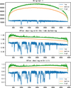 |
Fig. 1 Preprocessing: Three sub-images are features of the I image at three different stages in the preprocessing, i.e., the original data, the data with limb darkening corrected, and the data with tilt corrected. The three curves in each picture represent: the minimum (blue curve labeled by low in the figure), median (orange curve labeled by median in the figure), and maximum (green curve labeled by high in the figure) values of each column in the image, respectively. The horizontal axis represents the column of the image, and the unit is pixel. 0 is east of the sun, 4096 is west of the sun. The vertical axis is the value of each pixel. |
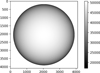 |
Fig. 2 Limb darkening background. Fitted from Stokes I image, the meaning of gray value is the same as I. The horizontal and vertical axis units are pixels. |
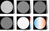 |
Fig. 3 Input images after preprocessing. All six input channels are normalized. The two velocity channels are stained with red and blue to represent Doppler movement. Red (greater than 0) means that trie sun and the probe are far away from each other, and blue means that they are close to each other. Since OBSVR is an observation parameter that; is only related to time, the entire image has the same value. ROTVR is the line of sight component of the rotation velocity of the solar surface. |
3 Method
3.1 Network
Residual network (ResNet) is a very popular CNN structure that was first published in 2016 (He et al. 2016). Manye studies have used this type of method in tackling astronomical problems.
Guo et al. (2021) used this method to the inversion of magnetic field. The design of the residual block in ResNet makes training deep networks possible. Shortcut connections in this structure can aptly solve the problems of vanishing gradients, exploding gradients, and degradation. In order to calculate the vector magnetic field, three parameters need to be obtained. The magnetic field parameters given by HMI level 2 data are field strength, inclination and azimuth. We use the longitudinal magnetic field, the transverse magnetic field and the azimuth as the output of the neural network prediction. The relationship between the two sets of vector magnetic field parameters is shown below:
 (7)
(7)
 (8)
(8)
Here, B is the field strength of the magnetic field, and θ is the inclination. Through Eqs. (7) and (8), we transform the magnetic field strength and inclination in the HMI magnetogram images into images of the longitudinal magnetic field Bl and the transverse magnetic field Bt and we use them as the target for neural network training.
We trained three neural networks for the three components: Bl, Bt, and the azimuthal angle φ of the vector magnetic field. Using different networks to predict different components instead of using one network to directly output three-channel images is helpful because it is difficult to design a reasonable loss function for three physical quantities with different units. Since it is difficult to balance the weights of different physical quantities in the loss function, it may appear that in order to reduce the loss for one physical quantity during training, the loss in terms of another quantity is greater. Therefore, the best method is to train different networks separately, even if these parameters may not be independent in the traditional inversion process.
Figure 4 shows the network structure we used in our study. Our model has 16 residual blocks, with two convolution layers in each block. There are a total of 34 convolutional layers in our model, each with 64 filter kernels except the last one. The final convolutional layer has only one output channel, so the final output of the network is a single-channel image. The size of the every kernel is 3 pixel × 3 pixel. The activation function we use is Leaky ReLU, defined as:
 (9)
(9)
where a is a very small value (e.g., in our model it is 0.01). Compared with the classic ReLU, the derivative of Leaky ReLU is not zero when it is less than zero. Thus, the gradient can still be propagated. This reduces the appearance of dead neurons (Maas et al. 2013).
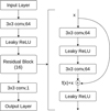 |
Fig. 4 ResNet model used in this study. |
3.2 Loss function and training
The commonly used loss functions in regression tasks are the mean squared error loss (MSE,L2 loss) and mean absolute error loss (MAE,L1 loss).
 (10)
(10)
 (11)
(11)
Here yi is the value of pixel i in target, and ŷi is the value of pixel i predicted by the network. Because MSE amplifies the error relatively, it can be solved for faster than with MAE. It can make the network converge quickly in the early stages of training. But MSE is not robust enough in the presence of many abnormal points. To consider the information at the strong field in greater depth, we define a weighted loss function:
 (12)
(12)
where loss(yi, ŷi) can be any loss function, such as (yi − ŷi)2 or |yi − ŷi|, and weight is the weight of the pixel, which is related to the field strength at this point. We designed such a weight function as:
 (13)
(13)
where p(B) is the probability of the field strength B in the training set. In the algorithm implementation, we divide the magnetic field strength into multiple bins and use the frequency of each bin as the probability of the magnetic field strength in the bin. Multiplying each pixel by such a weight, ω, is equivalent to expanding one pixel to the same ω. This is equivalent to undersample the case with a large number of times in the data set (weak magnetic field), and oversample the case with a small number of times (strong magnetic field). The strong magnetic field occupies a minority on the surface of the sun. If such weighting is not used, since the strong magnetic field accounts for a very small proportion, the contribution of the strong magnetic field to the loss function is also very small. Therefore, the optimizer can hardly consider the error of the strong magnetic field area when updating the network parameters. So, the network mainly learns the characteristics of the weak magnetic field area. In this way, it would be difficult for the network to accurately predict the magnetic field parameters of strong magnetic fields, and even though these areas account for a small proportion, they are still a very important part of solar physics research.
When training the azimuth angle, one important thing is that the azimuth angle is a periodic function. According to the definition of azimuth, the period of azimuth is 180°. We anticipate what the output azimuth angle is before correcting the 180° ambiguity, that is, the predicted transverse field direction can be the reverse of the actual direction. So, we then use the residual between prediction and target, which was used by Guo et al. (2021) when training the network of azimuth angle:
 (14)
(14)
That is, when the residual error between the prediction and the target is greater than 90°, the direction of reducing the loss function is meant to increase the residual to 180° instead of simply trying to reduce the residual.
The weighting of the loss function eventually brings on the problem of amplifying the error of the singularity of the magnetic field strength. In the solar magnetic field inversion, when the magnetic field intensity is very high, it will cause the spectral line to split too widely, pushing the peak of the polarization spectral line out of the scope of the detector’s observation (Hoeksema et al. 2014). At certain times, the Doppler effect will also intensify this problem. Therefore, when inverting the magnetic field, the inversion code may not converge in this case. There may be some discontinuous pixels in time or space in the inversion image, which would appear as sudden and sharp increase or decrease. These bad pixels mainly appear inside the sunspots, where the magnetic field is relatively large. Therefore, due to the weighting of pixels with large magnetic fields, the weight of these bad pixels is increased, which hinders the convergence of neural network training. Thus, we adopted several methods to remove these bad pixels; for example, by judging the relationship between a pixel and its eight neighborhoods. If all the pixels in the eight neighborhoods are much larger or much smaller than this pixel, then this point is deemed a bad pixel and this point is ignored when calculating the loss function. This can remove the influence of some bad pixels.
As previously mentioned, we cut input images to smaller shape in training process in order to load more data in a batch. The input image was cut into 256 pixel × 256 pixel. Data augmentation was then performed to randomly rotate, flip, or otherwise do no operation on the image. This makes the data more diversified and also makes the model have better generalization ability.
This work uses PyTorch 1.6.0 as the deep learning framework and also uses a graphics card to accelerate the calculation. Our model was trained on a NVIDIA Tesla V100-PCIE-16GB, with 5120 CUDA Cores and 640 Tensor Cores.
4 Results
We trained three networks to output longitudinal field strength, Bl, transverse field strength, Bt, and azimuth φ separately. We used these three networks to predict the full-disk data in the test set shown in Table 1. The data in the test set does not participate in training and is used to adjust network hyperparameters. In this section, we evaluate the difference between the prediction and the target and we analyze the error under different conditions in the discussion section. Since the convolution operation will diffuse the error outside the edge of the image inward, we excluded some pixels at the edge of the solar surface when performing the evaluation. Because the network has a total of thirty-four 3 × 3 convolutional layers, we discarded the 40-pixel (need to be greater than 34) ring on the edge of the solar surface.
In order to consider the output results in different situations, we used the network to predict 1665 full-disk data of the entire full-disk test set and counted the results. The data at 00:00:00 on December 6, 2015 is selected. In this section, we mainly discuss the characteristics of the full-disk magnetic field. The details of the activity regions are presented in the next section.
Data set.
4.1 Longitudinal field strength
For all the full disk data in the test set, the MAE between the prediction and the inversion of Bl is 3.68 G. However, considering the large number of quiet areas, the magnetic field strength itself is small, so the error of full disk will be small compared to that of the strong magnetic field. The error of the magnetic field is averaged in the statistics of the full disk. Therefore, our evaluation of the network predictions also needs to consider strong magnetic fields, such as pixels with an absolute value of Bl above 300 G. For pixels above 300 G, the MAE of Bl is 64.35, and the coefficient of determination R2 is 0.98. The definition of the coefficient of determination is as follows:
 (15)
(15)
where y̅ is the average value of target yi. This value is usually used to measure the correlation between the result of the ragres-sion and the target. The closer R2 is to 1 means the better tire result of the regression.
In Fig. 5, wife s how the full disk prediction and target of Bl, as well as the slices of the two active areas. The two active areas, shown are NOAA ARI2463 and NOAA ARS2462. The horizontal axis of the scatter plot is the inversion value, and the vertical axis iss the prediction output. From such a scatter plot, we can see the correlation between the prediction data and the target data. The 45° diagonal line is prediction = target. So the closer the point distribution is to this line means the better the regression effect.
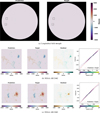 |
Fig. 5 Result of the longitudinal field. (a) Full disk: longitudinal magnetogram at 00:00:00 on December 6, 2015, both images are 4096 × 4096 pixels. Left: prediction from neural network. Right: inversion result from VFISV. Two activity regions are marked with black boxes. (b)Active region NOAA AR12462 in (a). From left to right: prediction of the neural network; inversion result from VFISV; Residual of the prediction and inversion; Scatter diagram, the horizontal axis is the target, and the vertical axis is the prediction. (c) The active region NOAA AR12463 in (a). Same as (b).– |
4.2 Transverse field strength
The measurement accuracy of the transverse field is lower than that of the longitudinal field. The MAE of the error between the predicted Bt and the inversion result is 28.08 G. For pixels above 300G, the MAE of the Bt error is 62.08 G, and the R2 is 0.87. It is worth noting that there is a minimum value and the transverse field pre dictions given by the neural network are all greater than this minimum value. The minimum value is around 60 G. Trie interesting thing is that our neural network does not set the minimum value of output and there are pixels smaller than this minimum in lite target image in training and testing. This error should come from the effect of the photon noise (Borrero & Kobel 2011). Since the signals of Stokes Q and U are weaker, thr signat-to-noise ratio (S/N) is also lower. Therefore, there is a lot of noise in the Q and U signals from the weak field, so that the weaker trans vert e field of inversion is largely from the noise.
Similarly, we show the full disk prediction of the transverse field and two active regions in Fig. 6. It can be seen in the scatter plot that there is a minimum value for the prediction of the transverse field. In general, the prediction results for the transverse field in the strong area are still good enough.
4.3 Azimuth
Similarly to the tran sverse field, in the quiet zone that o ccup ies a large area on the solar surface, due to the low S/N of the Q and U signals, there is a lot of noise in the azimuth obtained by the inversion. This also leads to the different pюrformance of the neural network’s prediction of the azimuth angle in the quiet and active regions. For the full disk:, the MAE of the error between the azimuth prediction and the target is 42.16°. For pixels with a transverse field strength of 300 G or more, the MAE of the azimuth error is 12.29°.
In Fig. 7, we show the azimuth of the full disk and two active regions. It can clearly be seen that in the residual map, the sunspots area are mostly close to white. Interestingly, a large number of points are also gathered near the upper left corner (0, 180l and trie lower right corn er (180, 0) of the scatter plot.
Since the period of the azimuth angle is 180°, 0 and 180 are the same before the 180° disambiguation of the azimuth angle. Therefore, when we train the azimuth angle, we use the aforementioned loss function Eq. (14), which causes the points that are too far from the 45° line in the scatter plot to gather in two corners.
5 Discussion
The main purpose of our research is to verify whether a neural network calibration can solve the wavelength drift problem of calibration under a single wavelength. In this section, we examine the accuracy of neural network predictions at different relative velocities. There are two main sources of wavelength shift in polarization observations, namely, the rotation velocity of the sun and the orbital velocity of the satellite. It is worth noting that a key role is played by the line-of-sight component of each velocity.Therefore, the velocities mentioned later are all line-of-sight components. The velocity is set to be positive when they are moving away from each other, to be consistent with the JSOC keys.
5.1 OBSVR
In Fig. 8, we show the results of the neural network prediction of the longitudinal field strength Bl at different velocities. The two events selected have maximum positive and negative velocities, respectively, among the 120 datasets on December 6, 2015. The velocity of observer in radial direction OBSVR is 1738.65 ms−1 at 01:00 and −2208.77 ms−1 at 13:00, respectively. In Fig. 8, we also show the image of the circularly polarized signal Stokes V. Here, V has been normalized by Stokes I. The single-wavelength calibration under the weak field approximation linearly approximates the longitudinal field as a function of V, and we can see from the scatter diagram of V-Target that the linear relationship with V is no longer valid while the field strength increases. Another interesting point is that at different velocities, the scatter plots of V-Target show different shapes. This is derived from the change in the observed wavelength. The existence of OBSVR makes the actually observed wavelength points at different wavelength positions on the spectrum. The calibration relations at different positions are obviously different, which causes the difference in the shape of the scatter plot. It is worth noting that at different velocities, the shapes of the scatter plots for V-Prediction and V-Target have maintained consistent changes. This is strong evidence that the neural network has learned the nonlinear calibration relationship under different wavelength shifts. We counted the variation of the error at different velocities during the day. For the longitudinal magnetic map, the maximum MAE error of Bl is 4.90 G and the minimum is 3.64G; the maximum MAE error of Bt is 62.79 G, and the minimum is 42.52 G. In addition, we tracked and observed the error changes in the active area. The statistics of NOAA AR12463 and NOAA AR12462 are respectively counted.
In Fig. 9, we show the relationship between MAE and OBSVR of the prediction results of the magnetic field components of the whole solar surface and the two active regions on December 6, 2015. The error of the active region is greater than the error of the full solar surface because the field strength of the active area is much greater than the field strength of the active region, making the absolute error larger. This does not mean that the calibration result in the strong field area is worse than that in the weak field area. The error of the prediction results varies with OBSVR. We consider the range of this error that varies with OBSVR as a reference for the error brought by OBSVR in the system. The MAE floating range of Bl in the two active regions is about 10 G, and the MAE floating range of Bt is also less than 25 G. The error fluctuation range of Bl and Bt predicted in the active area is smaller than the change of the average field strength of the active area with the LoS velocity. This demonstrates that the training of the neural network has reduced the error caused by OBSVR in the prediction to the level of the error caused by OBSVR in the data itself. The statistics of the azimuth angle is the selected pixels with a transverse field above 300 G. This is because the previously mentioned error in the azimuth inversion in the quiet zone means it is optimal to only count the azimuth of the strong magnetic field.
5.2 ROTVR
We also investigated the influence of the solar rotation on the calibration results. Similarly, what affects the observation is its line-of-sight component, namely, the ROTVR. The difference in the rotation velocity of the sun is reflected in the spatial distribution of the image. As shown in Fig. 3f, from east (left of image) to west (right of image) on the solar surface, the spectral line gradually shifts from blue to red shift. Hence, we found two active areas in the test set, located on the east and west of the sun. One activity region is NOAA AR12463 on December 6, 2015, and the other is NOAA AR12600 on October 17, 2016. In Fig. 10, we show the positions of these two active regions as the areas enclosed by the black boxes in the picture. The ROTVR in the central area of NOAA AR12463 at the moment in the figure is about −1800 m s−1, and the ROTVR in the central area of NOAA AR12104 is about 1650 ms−1. This is the first magnetogram in each date at 00:00. With the rotation, the absolute values of ROTVR of NOAA AR12111 and NOAA AR12104 gradually decrease and increase respectively. In Fig. 11, the errors of the magnetic field parameters of the two active regions are counted as a function of OBSVR. The errors of the two active regions show opposite trends with the changes of OBSVR. This is because the two active regions are in opposite ROTVR directions. The difference between the maximum value of the MAE of Bl of the two active regions is 3.15 G, and the difference of the minimum value is 4.05 G; the difference of the maximum of MAE of Bt is 35.16 G, and the difference of minimum MAE is 8.95 G. It can be seen that the error range brought by ROTVR is slightly smaller than the error brought by OBSVR. It is interesting that the azimuth error of NOAA AR12600 becomes larger as OBSVR increases. This means that the superposition of the two relative motion further enlarges the wavelength shift effect and thus increases the error. We also show the error of the results obtained using linear calibration for these two active regions. The variation trend of the error of linear calibration with OBSVR is the same as the result that comes from ANN, showing different trends under different ROTVR. Moreover, the error of linear calibration is significantly larger than the result of ANN. This shows that ANN calibration is better than linear calibration and performs better at the edge of the Sun.
5.3 Wavelength shift
Earlier in this paper, we discuss the impact of two line-of-sight velocity terms on the observation accuracy. We hope to further and more directly discuss the effect of the two velocities on the calibration error. According to the Doppler formula:
 (16)
(16)
where f′is the frequency received by the observer and ƒ is the frequency emitted by the wave source; υ0 is the velocity of the observer’s movement and υs is the velocity of the wave source movement, both of which are positive when the observer and wave source arre moving away from each other (and vise verse). After substituting the terms with OBSVR, ROTVR, and the velocity of light, c, the measurement of the wavelength change can be obtained:
 (17)
(17)
wehere λ is trie wavelength emitted by the wave source, 6173.34 Å. In particulan, Eq. (17) is ai first-order approximation that ignores high-order small terms. Assuming that the maximum value of ROTVR and OBSVR is ±3000 ms−1, the maximum error of Δλ obteined by Eq. (17) is about 6 × 10⁻⁷ Å. Therefore, the accuracy of calculatingthe wavelength shift in this way is sufficient, so we can directly add the two velocity terms to get the wavelength shift when we investigate the influence of velority.
Figure 12 calculates the MAE under different VR on each full disk in the test set, and then displays the MAE of each full disk: as a 2D histogram about VR. Here, VR is the total relative velocity of a point on the image and the detector:
 (18)
(18)
Horizontal axis in the figure also identify the wavelength shift corresponding to the VR in the figure. As mentioned earlier, the quiet zone has a low absolute error due to its low intensity, which ends up reducing trie average error of all pixds. In addition: due to the low S/N of the linearly polarized signal under a weak mag-netic field, the horizontal field and azimuth angle measurement accuracy of these pixels is poor. Therefore, in order to accurately examine the variation of error with VR, in our statistics, the error of Bl only counts the pixels whose absolute value of Bl is above 100 G; the error of Bt and azimuth only counts the pixels whose Bt is above 300 G. In addition, all bad pixels are ignored in the statistics. The bad pixel algorithm in the loss function mentioned above is used. It can be seen that the MAE of Bl varies by 25 G with VR ranging from 0 to ±4000 ms−1. Interestingly, the error of Bt and azimulh reaches the peak value at ±2000 ms−1, and the error decreases as the velocity continues to increase. Trie Bt and azimuth errors at the peak are about 50 G and 15° higher than those at 0 ms−1.
To examine the role of the velocity channels in the network input, we trained the network without input OBSVR. The inputs to these networks are only five channels, that is, Stokes IQUV and ROTVR. We find that the predictions of such a network suffer from background noise. In Fig. 13, we show an example of this, which is the residual between the network prediction and the target, with a distinctly uneven background.
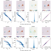 |
Fig. 8 Longitudinal magnetic field of NOAA AR12463. (a) Result at 01:00, OBSVR is 1738.65 m s−1; (b) is at 133:00, OBSVR is −2208.77 m s−1. The first row of sub-images of (a) and (b) are the prediction of NOAA AR12463; the inverted image as the target; the residual error between the prediction and the target; the circular polarization signal Stokes V related to the longitudinal magnetic field. The first two pictures in the second row of subpicturec aire scatter plots of V and the longitudinal field. The horizontal axis; is V, and the vertical axis is the longitudinal field. The vertical axis of the left first picture in the row two is the prediction of the neural network, and the vertical axis of the second picture is the target. The third picrure in trie second row is a statistical histogram of errors, and the unit of the horizontal axis is G. The fourth picture is a scatter histogram of prediction and target. The horizontal axis is target and the verticai axis is prediction, and both units are G. |
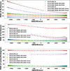 |
Fig. 9 MAE changes with OBSVR. The three sets of data are the MAE errors of full disk, NOAA AR12462, and NOAA AR12463 on December 6, 2015. From top to bottom: errors of the longitudinal magnetic field, the transverse magnetic field, and the azimuth angle. The results of linear calibration are also added for comparison and plotted as stars. |
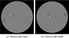 |
Fig. 10 Position of the active area on the sun surface. (a) The LoS magnetic map at 00:00 ont December 6, 22015, where the framed part is NOAA AR12463. (b) The LoS magnetic map at 00:00 on October 17, 2016, where the framed part is NNOAA AR12600. |
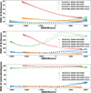 |
Fig. 11 Change in MAE with OBSVR under different ROTVR. Same as Fig. 9. Two sets A data are: NOAA AR12463 on December 6, 2015 and NOAA AR12600 on October 17, 2016, along with the error of the magnetic field obtained by linear calibration. |
6 Conclusion
In this work, our aim is to verify whether the neural network is effective for the vector magnetic field calibration method in the presence of wavelength drift. We selected the 720s data series of HMI/SDO as thee training and test data. We used the polarization image of the second wavelength position from the level 1 data of the HMI as the input of the neural network, and we used the vector magnetogram of the HMI as the target output: for the neural network. We converted the total field strength, inclination angle and azimuth angle of the three components of the vector magnetic field into longitudinal magnetic field, transverse magnetic field, and azimuth angle as the target in practical applications.
Our network uses a modified ResNet (without the Batch-Norm layer). At the end of the network used to output azimuth, a layer of transformation was added to limit the network output to the range of [0, 180). There are no learnable parameters in this layen We designed a set of pre processing methods to process the raw data. We removed a variety of uneven backgrounds in the Stokes I image. And the normalization operations were carried out on Stokes I, Q, U and V.
The relative motion between the probe and the Sun causes the wavelength of the spectral line to shift when observing the magnetic field. Since our input is a single-wavelength polarization signal, a complete spectral line Stokes profile cannot be obtained, so trie wavelength shift will bring on calibration errors. There are two main sources for the wavelength shift, namely, the Sun’s rotation velocity and the orbital velocity of the satellite.
In order to obtain the calibration results that adapt to multiple wavelength drift situations, we put the velocity term that causes the wavelength drift into the input data of the neural network.
In view of the characteristics ot the data in rhe training, we designed some special loss function corrections. Since there are fewer samples in the strong magnetic field area, we did not want the network to learn only the weak magnetic field characteristics that account for the majority of the number of samptes; thus, we weighted different magnetic field strengths. This is equivalent to re-sampling the data set.
To examine thee overall performance of our neural network, we tested it on a full disk test set of 1665 data. For the entire test set: the error (MAE) of Bl and Bt on thee whole disk are 4.29 G and 30.99 G, respectively. In addition, considering the regions where Bt is above 300 G, the MAE of azimuth is 14.34°. Due to the low S/N of Stokes Q and U signals in the quiet region, the corresponding errors of the transverse field and azimuth angle are relatively large. Therefore, it is only meaningful for the azimuth to investigate regions with strong field strength.
The purpose of our work is to explore whether the neural network method can meet the needs of vector magnetic field calibration with wavelength drift. We separately examined the effects of the Sun’s rotation velocity and orbital velocity. We also counts the errors caused by wavelength drift at different total relative motion velocities for the entire test set. In nonextreme cases, the errors of B1, Bt and azimuth will increase with the VR by up to 25 G, 50 G, and 15°. When the total velocity is extremely high, the wavelength shift is about twice the distance between each of the six wavelength points observed by the HMI. This leads to the disappearance of the signal and, thus, the error would rise rapidly. This is irreversible under single-wavelength calibrations. However, this situation only accounts for a very small number of magnetic field measurements and neural network single-wavelength calibration is acceptable in most cases.
By analyzing the errors in various situations, we believe that the neural network has the ability to perform the single-wavelength calibration task of the vector magnetic field with wavelength shift, but there are still some limitations.
The first is the unbalanced field strength of the training set and the problem of bad pixels. At present, a better method is to weight the pixels to achieve the effect of a resampled data set. However, the weights need to be designed according to the characteristics of the data set. In addition, the impact of bad pixels needs to be considered. The high weight of strong magnetic fields will increase the misleading training caused by these strong magnetic fields. We adopted a conservative bad pixel algorithm to ascertain that the removed pixels are indeed bad pixels, but we did not remove all the bad pixels.
The second is the distribution and data volume of OBSVR in the training set. The data set used for training should include full disk images at various orbital velocities. This is difficult to do through resampling because it is related to the observation time. It is also difficult to establish a data set with sufficient samples at various Doppler velocities.
Last but not least, the neural network calibration method is data-driven. The prediction accuracy of the ANN in the regression task depends on the accuracy of the target used for training, and cannot be higher than the accuracy of the target. Therefore, the observation accuracy used for calibration will largely determine the accuracy of the neural network.
In conclusion, our work verifies the finding that it is feasible to use neural networks for single-wavelength vector magnetic field calibration tasks with wavelength drift. We will conduct further work to further improve the accuracy of network prediction as well as to verify the feasibility of neural network calibration for the FMG/ASO-S mission.
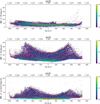 |
Fig. 12 2D histogram of MAE error and relative motion VR in the test set. Red line is the median MAE at different relative velocities. From top to bottom: MAEerrors of the longitudinal magnetic field, the transverse magnetic field, and the azimuth angle. The horizontal axis at the top of each graph indicates the wavelength shift Δλ corresponding to the relative velocity. Color bars show the bin counts. |
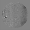 |
Fig. 13 Residual of the prediction from the network without OBSVR. This map is at 13:00 on July 8, 2017. |
Acknowledgements
This work is supported by National Natural Science Foundation of China (Grant Nos. 12073077, 11427901, 11773038, U1831107, 1210030183), and the Strategic Priority Research Program on Space Science, the Chinese Academy of Sciences (Grant Nos. XDA15320302, XDA15052200, XDA15320102), and Beijing Natural Science Foundation(Grant No.1222029), and National Key R&D Program of China (Grant No. 2021YFA1600500).
References
- Ai, G.-X., Li, W., & Zhang, H.-Q. 1982, Chinese Astron. Astrophys., 6, 129 [CrossRef] [Google Scholar]
- Asensio Ramos, A., & de la Cruz Rodríguez, J. 2015, A&A, 577, A140 [NASA ADS] [CrossRef] [EDP Sciences] [Google Scholar]
- Asensio Ramos, A., & Díaz Baso, C. J. 2019, A&A, 626, A102 [NASA ADS] [CrossRef] [EDP Sciences] [Google Scholar]
- Bai, X. Y., Deng, Y. Y., & Su, J. T. 2013, Sol. Phys., 282, 405 [CrossRef] [Google Scholar]
- Bai, X. Y., Deng, Y. Y., Teng, F., et al. 2014, MNRAS, 445, 49 [Google Scholar]
- Bai, X., Liu, H., Deng, Y., et al. 2021, A&A, 652, A143 [NASA ADS] [CrossRef] [EDP Sciences] [Google Scholar]
- Borrero, J. M., & Kobel, P. 2011, A&A, 527, A29 [NASA ADS] [CrossRef] [EDP Sciences] [Google Scholar]
- Borrero, J. M., Tomczyk, S., Kubo, M., et al. 2011, Sol. Phys., 273, 267 [Google Scholar]
- Carroll, T. A., & Staude, J. 2001, A&A, 378, 316 [NASA ADS] [CrossRef] [EDP Sciences] [Google Scholar]
- Carroll, T. A., Kopf, M., & Strassmeier, K. G. 2008, A&A, 488, 781 [NASA ADS] [CrossRef] [EDP Sciences] [Google Scholar]
- Centeno, R., Schou, J., Hayashi, K., et al. 2014, Solar Phys., 289, 3531 [NASA ADS] [CrossRef] [Google Scholar]
- Deng, Y. Y., Zhang, H. Y., Yang, J. F., et al. 2019, Res. Astron. Astrophys., 11, 157 [CrossRef] [Google Scholar]
- Gan, W. Q., Zhu, C., Deng, Y. Y., et al. 2019, Res. Astron. Astrophys., 19, 156 [CrossRef] [Google Scholar]
- Guo, J., Bai, X., Deng, Y., et al. 2020, Sol. Phys., 295, 5 [NASA ADS] [CrossRef] [Google Scholar]
- Guo, J., Bai, X., Liu, H., et al. 2021, A&A, 646, A41 [NASA ADS] [CrossRef] [EDP Sciences] [Google Scholar]
- Hagyard, M. J., Adams, M. L., Smith, J. E., & West, E. A. 2000, Sol. Phys., 191, 309 [Google Scholar]
- Hale, G. E. 1908, ApJ, 28, 315 [Google Scholar]
- He, K., Zhang, X., Ren, S., & Sun, J. 2016, in 2016 IEEE Conference on Computer Vision and Pattern Recognition (CVPR), 770 [Google Scholar]
- Higgins, R. E. L., Fouhey, D. F., Zhang, D., et al. 2021, ApJ, 911, 130 [NASA ADS] [CrossRef] [Google Scholar]
- Hoeksema, J. T., Liu, Y., Hayashi, K., et al. 2014, Sol. Phys., 289, 3483 [Google Scholar]
- Hornik, K. 1991, Neural Netwo., 4, 251 [CrossRef] [Google Scholar]
- Jefferies, J., Lites, B. W., & Skumanich, A. 1989, ApJ, 343, 920 [Google Scholar]
- Li, H., Xu, Z., Qu, Z., & Sun, L. 2019, ApJ, 875, 127 [Google Scholar]
- Maas, A. L., Hannun, A. Y., & Ng, A. Y. 2013 Proc. icml, 30, 3 [Google Scholar]
- Norton, A. A., Graham, J. P., Ulrich, R. K., et al. 2006, Sol. Phys., 239, 69 [NASA ADS] [CrossRef] [Google Scholar]
- Pesnell, W. D., Thompson, B. J., & Chamberlin, P. C. 2012, Sol. Phys., 275, 3 [Google Scholar]
- Ruiz Cobo, B., & del Toro Iniesta, J. C. 1992, ApJ, 398, 375 [Google Scholar]
- Schou, J., Scherrer, P. H., Bush, R. I., et al. 2012, Sol. Phys., 275, 229 [Google Scholar]
- Skumanich, A., & Lites, B. W. 1987, ApJ, 322, 473 [Google Scholar]
- Socas-Navarro, H. 2001, in Astronomical Society of the Pacific Conference Series, 236, Advanced Solar Polarimetry – Theory, Observation, and Instrumentation, ed. M. Sigwarth, 487 [Google Scholar]
- Socas-Navarro, H. 2003, Neural Networks, 16, 355, Neural Network Analysis of Complex Scientific Data: Astronomy and Geosciences [Google Scholar]
- Socas-Navarro, H. 2003, Neural Netw., 16, 355 [NASA ADS] [CrossRef] [Google Scholar]
- Stenflo, J. 1994, Solar Magnetic Fields: Polarized Radiation Diagnostics, 189 [Google Scholar]
- Su, J., & Zhang, H. 2004, Sol. Phys., 222, 17 [Google Scholar]
- Su, J.-T., Bai, X.-Y., Chen, J., et al. 2019, Res. Astron. Astrophys., 19, 161 [Google Scholar]
- Sykes, J. B. 1953, MNRAS, 113, 198 [NASA ADS] [CrossRef] [Google Scholar]
- Teng, F. 2015, Sol. Phys., 290, 2693 [Google Scholar]
- Timothy, A. F., Krieger, A. S., & Vaiana, G. S. 1975, Solar Phys., 42, 135 [NASA ADS] [CrossRef] [Google Scholar]
- Tsuneta, S., Ichimoto, K., Katsukawa, Y., et al. 2008, Sol. Phys., 249, 167 [Google Scholar]
All Tables
All Figures
|
Fig. 1 Preprocessing: Three sub-images are features of the I image at three different stages in the preprocessing, i.e., the original data, the data with limb darkening corrected, and the data with tilt corrected. The three curves in each picture represent: the minimum (blue curve labeled by low in the figure), median (orange curve labeled by median in the figure), and maximum (green curve labeled by high in the figure) values of each column in the image, respectively. The horizontal axis represents the column of the image, and the unit is pixel. 0 is east of the sun, 4096 is west of the sun. The vertical axis is the value of each pixel. |
| In the text | |
|
Fig. 2 Limb darkening background. Fitted from Stokes I image, the meaning of gray value is the same as I. The horizontal and vertical axis units are pixels. |
| In the text | |
|
Fig. 3 Input images after preprocessing. All six input channels are normalized. The two velocity channels are stained with red and blue to represent Doppler movement. Red (greater than 0) means that trie sun and the probe are far away from each other, and blue means that they are close to each other. Since OBSVR is an observation parameter that; is only related to time, the entire image has the same value. ROTVR is the line of sight component of the rotation velocity of the solar surface. |
| In the text | |
|
Fig. 4 ResNet model used in this study. |
| In the text | |
|
Fig. 5 Result of the longitudinal field. (a) Full disk: longitudinal magnetogram at 00:00:00 on December 6, 2015, both images are 4096 × 4096 pixels. Left: prediction from neural network. Right: inversion result from VFISV. Two activity regions are marked with black boxes. (b)Active region NOAA AR12462 in (a). From left to right: prediction of the neural network; inversion result from VFISV; Residual of the prediction and inversion; Scatter diagram, the horizontal axis is the target, and the vertical axis is the prediction. (c) The active region NOAA AR12463 in (a). Same as (b).– |
| In the text | |
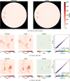 |
Fig. 6 Result of the trans verse field. Details are the same as in Fig. 5. |
| In the text | |
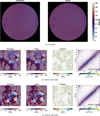 |
Fig. 7 Result of the azimuth angle. Details are the same as in Fig. 5. |
| In the text | |
|
Fig. 8 Longitudinal magnetic field of NOAA AR12463. (a) Result at 01:00, OBSVR is 1738.65 m s−1; (b) is at 133:00, OBSVR is −2208.77 m s−1. The first row of sub-images of (a) and (b) are the prediction of NOAA AR12463; the inverted image as the target; the residual error between the prediction and the target; the circular polarization signal Stokes V related to the longitudinal magnetic field. The first two pictures in the second row of subpicturec aire scatter plots of V and the longitudinal field. The horizontal axis; is V, and the vertical axis is the longitudinal field. The vertical axis of the left first picture in the row two is the prediction of the neural network, and the vertical axis of the second picture is the target. The third picrure in trie second row is a statistical histogram of errors, and the unit of the horizontal axis is G. The fourth picture is a scatter histogram of prediction and target. The horizontal axis is target and the verticai axis is prediction, and both units are G. |
| In the text | |
|
Fig. 9 MAE changes with OBSVR. The three sets of data are the MAE errors of full disk, NOAA AR12462, and NOAA AR12463 on December 6, 2015. From top to bottom: errors of the longitudinal magnetic field, the transverse magnetic field, and the azimuth angle. The results of linear calibration are also added for comparison and plotted as stars. |
| In the text | |
|
Fig. 10 Position of the active area on the sun surface. (a) The LoS magnetic map at 00:00 ont December 6, 22015, where the framed part is NOAA AR12463. (b) The LoS magnetic map at 00:00 on October 17, 2016, where the framed part is NNOAA AR12600. |
| In the text | |
|
Fig. 11 Change in MAE with OBSVR under different ROTVR. Same as Fig. 9. Two sets A data are: NOAA AR12463 on December 6, 2015 and NOAA AR12600 on October 17, 2016, along with the error of the magnetic field obtained by linear calibration. |
| In the text | |
|
Fig. 12 2D histogram of MAE error and relative motion VR in the test set. Red line is the median MAE at different relative velocities. From top to bottom: MAEerrors of the longitudinal magnetic field, the transverse magnetic field, and the azimuth angle. The horizontal axis at the top of each graph indicates the wavelength shift Δλ corresponding to the relative velocity. Color bars show the bin counts. |
| In the text | |
|
Fig. 13 Residual of the prediction from the network without OBSVR. This map is at 13:00 on July 8, 2017. |
| In the text | |
Current usage metrics show cumulative count of Article Views (full-text article views including HTML views, PDF and ePub downloads, according to the available data) and Abstracts Views on Vision4Press platform.
Data correspond to usage on the plateform after 2015. The current usage metrics is available 48-96 hours after online publication and is updated daily on week days.
Initial download of the metrics may take a while.