| Issue |
A&A
Volume 697, May 2025
|
|
|---|---|---|
| Article Number | A28 | |
| Number of page(s) | 15 | |
| Section | The Sun and the Heliosphere | |
| DOI | https://doi.org/10.1051/0004-6361/202553918 | |
| Published online | 06 May 2025 | |
Deconvolution of SDO/HMI intensity and the vector magnetic field to achieve Hinode/SOT-SP data quality
1
Astronomical Institute of the Czech Academy of Sciences, Fričova 298, 25165 Ondřejov, Czech Republic
2
Astronomical Institute, Charles University, V Holešovičkách 2, 18000 Prague, Czech Republic
3
Institut für Sonnenphysik (KIS), Georges-Köhler-Allee 401A, 79110 Freiburg im Breisgau, Germany
⋆ Corresponding author: This email address is being protected from spambots. You need JavaScript enabled to view it.
Received:
27
January
2025
Accepted:
21
March
2025
Abstract
Context. The SDO/HMI instrument provides continuous full-disk observations with a high temporal cadence but moderate spatial resolution. In contrast, Hinode/SOT-SP observes the Sun with high spatial resolution but at a low temporal cadence and within a limited field of view.
Aims. This study seeks to enhance SDO/HMI observations by applying deconvolution techniques, specifically to the continuum intensity and full vector magnetic field in a local reference frame. Hinode datum, used as a training set, helps the model improve the resolution of HMI data to a Hinode-like level.
Methods. We use deep residual convolutional neural networks trained on HMI-like and SOT-SP observations. The HMI-like observations utilise the SOT-SP observations and the exact HMI point-spread function and noise realisation.
Results. The trained model successfully deconvolves both the intensity and the vector magnetic field. The model predictions and SOT-SP observations show the same level of detail. The root mean square difference between the two is 0.02 quiet-Sun level for intensity and between 40 and 45 G for vector magnetic field that is below the disambiguation noise level.
Conclusions. Our model effectively addresses disambiguation noise and enables the deconvolution of the full vector magnetic field. Additionally, the modelled deconvolution provides enhanced results compared to the standard HMI pipeline products.
Key words: methods: numerical / Sun: magnetic fields / Sun: photosphere
© The Authors 2025
 Open Access article, published by EDP Sciences, under the terms of the Creative Commons Attribution License (https://creativecommons.org/licenses/by/4.0), which permits unrestricted use, distribution, and reproduction in any medium, provided the original work is properly cited.
This article is published in open access under the Subscribe to Open model. This email address is being protected from spambots. You need JavaScript enabled to view it. to support open access publication.
1. Introduction
The Hinode satellite (Kosugi et al. 2007) and the Solar Dynamics Observatory (SDO, Pesnell et al. 2012) are complementary solar observation missions designed to study the solar magnetic field and its influence on solar activity. Hinode, launched by JAXA in 2006, utilises the Solar Optical Telescope Spectro-Polarimeter (SOT-SP, Tsuneta et al. 2008; Lites et al. 2013), which specialises in high-resolution spectro-polarimetric observations of localised regions on the solar surface, typically focusing on active regions. SOT-SP scans these regions, resulting in a temporal resolution of the order of hours. SDO, launched by NASA in 2010, is equipped with three instruments, including the Helioseismic and Magnetic Imager (HMI, Scherrer et al. 2012; Schou et al. 2012), which provides continuous, full-disk observations of the solar photospheric magnetic field and Doppler velocity. HMI is particularly well-suited for large-scale studies, utilising Dopplergrams for helioseismology and vector magnetic field data to investigate sunspot evolution and global magnetic activity. Although SOT-SP captures fine details of magnetic fields in specific regions with high spatial resolution, HMI offers broader spatial and temporal coverage, making the two instruments highly complementary for studying solar magnetic dynamics across spatial and temporal scales. This study aims to enhance HMI data by applying neural network-based deconvolution techniques to convert them into Hinode-like resolution. Hinode data, degraded to HMI resolution, are used as a training set, enabling the model to restore HMI data to a higher resolution. The model allows for the enhancement of full-disk, high-cadence HMI data to Hinode-like data.
Deconvolution is a mathematical technique used to restore or reconstruct signals or images that have been degraded by a point-spread function (PSF). This degradation typically occurs in observational systems due to instrument limitations, atmospheric effects, or other sources of distortion. In its simplest form, deconvolution aims to reverse the convolution process, where the ideal signal or image is combined with the PSF. However, direct inversion methods can be unstable, especially in the presence of noise, as they tend to amplify high-frequency components. To address this, regularised approaches, such as Wiener deconvolution, are commonly employed. These methods balance the restoration of the signal with noise suppression, ensuring more stable and reliable solutions. Deconvolution methods are widely applied in various fields, including astronomy, medical imaging, and remote sensing, where recovering fine details from blurred data is crucial for scientific analysis and interpretation.
Artificial neural networks (ANN, Goodfellow et al. 2016) are empirical computational models inspired by the structure and function of biological neural systems, designed to process and analyse complex data. They consist of interconnected layers of artificial neurons, where each neuron applies a mathematical function to its input and passes the result to the next layer. Neural networks are particularly effective at identifying patterns and relationships in large datasets. Due to their flexibility, they have been successfully used to solve very different tasks in astrophysics, from exoplanet detection (Valizadegan et al. 2022), over asteroid classification (Penttilä et al. 2021), to coronal magnetic field extrapolation (Jarolim et al. 2023), to name a few.
Recently, several studies have been conducted using neural networks to improve the resolution of HMI data. Díaz Baso & Asensio Ramos (2018) demonstrated that neural network-based deconvolution outperforms traditional methods in both image enhancement and artefact reduction. They trained the ENHANCE model using simulated data and an approximated HMI PSF. This model is capable of deconvolving intensitygrams and line-of-sight magnetograms. Rahman et al. (2020) found that neural networks are particularly effective in improving the resolution of HMI line-of-sight magnetograms. Wang et al. (2024) introduced the advanced SUPERSYNTHIA model, which was trained to map the HMI Stokes vector data to the vector magnetic field in a local reference frame, calculated using the SOT-SP pipeline. Despite careful co-alignment of the HMI and SOT-SP observations, they faced difficulties due to imprecise pointing information from the Hinode satellite and the evolution of the solar surface during Hinode’s observations. This imprecise co-alignment made pixel-to-pixel comparisons between the processed HMI data and the Hinode pipeline outputs challenging.
This study introduces an independent neural network model trained to convert HMI observations into Hinode-like intensitygrams and vector magnetic fields, where the term ‘observations’ refers to the outputs of processing pipelines rather than raw satellite data. To address the challenge of co-aligning HMI and SOT-SP data, we simulate this process by degrading SOT-SP observations using the exact HMI PSF and noise statistics. By incorporating precise noise contributions, the model can reconstruct HMI data without amplifying the noise. We resampled the HMI data to match the pixel resolution of SOT-SP. The model then performs deconvolution on the resampled data, restoring its quality to a level comparable to that of SOT-SP. This approach enables detailed studies of flux emergence and active region formation over extended timescales while preserving HMI’s broad spatial and temporal coverage. By combining the advantages of HMI’s full-disk coverage and high temporal resolution with enhanced detail, this method facilitates more comprehensive investigations of solar magnetic field dynamics and activity across multiple spatial and temporal scales, including high-resolution observations of both flux emergence and decay phases. While Hinode SOT-SP provides high-resolution observations of the magnetic field, its limited field of view and discontinuous coverage primarily capture already-developed active regions rather than their initial emergence.
The neural network model used in this work was written in Python using the TensorFlow/Keras (Abadi et al. 2015; Chollet et al. 2015) library. All code and pretrained models are available in the GitHub repository HMI_to_SP1, version v1.0, under the MIT license.
2. Deconvolution
Deconvolution is a data restoration technique that aims to reconstruct high-frequency details that have been corrupted by a non-ideal point-spread function. For 2D data, where the observed data f, the ideal data z, the constant PSF h, and the additive noise n are involved, the relationship between these quantities is given by the following equation:
 (1)
(1)
where * denotes the convolution operator.
The formal solution to this equation, assuming perfect knowledge of the PSF and noise realisation, is expressed as:
![Mathematical equation: $$ \begin{aligned} z(x, y) = \mathcal{F} ^{-1}\left[\frac{F(k_x, k_y) - N(k_x, k_y)}{H(k_x, k_y)}\right], \end{aligned} $$](/articles/aa/full_html/2025/05/aa53918-25/aa53918-25-eq2.gif) (2)
(2)
where ℱ−1 represents the inverse Fourier transform and F(kx, ky), H(kx, ky), and N(kx, ky) are the Fourier transforms of f(x, y), h(x, y), and n(x, y), respectively.
In practice, when the exact realisation of the noise is unknown, applying the formal solution can lead to an amplification of high-frequency noise. When the statistical distribution of the noise is known, as is the case with SDO/HMI, we can use the statistical properties of the noise along with the known PSF to obtain a more accurate approximate solution  , reducing the amplification of high-frequency noise.
2.1. Wiener algorithm
The standard Wiener deconvolution (Wiener 1949) provides an approximate solution by filtering the observed data in the frequency domain. The estimated solution and the Wiener filter G(kx, ky) are defined as:
![Mathematical equation: $$ \begin{aligned} \hat{z}(x, y)&= \mathcal{F} ^{-1}\left[G(k_x, k_y) F(k_x, k_y)\right],\end{aligned} $$](/articles/aa/full_html/2025/05/aa53918-25/aa53918-25-eq4.gif) (3)
(3)
 (4)
(4)
Here, H*(kx, ky) is the complex conjugate of H(kx, ky) and 𝔼[X] represents the expected value of the quantity X. We note that the ideal signal’s power spectral density 𝔼|Z(kx,ky)|2 is unknown. In practice, an estimate or assumption of the signal’s power spectrum is typically used, while the noise power spectral density 𝔼|N(kx,ky)|2 and the PSF H(kx, ky) are known or can be estimated. The Wiener filter works by balancing the signal’s power spectrum with the noise’s power spectrum to reduce the amplification of noise, particularly in high-frequency regions.
2.2. Richardson–Lucy algorithm
Unlike Wiener deconvolution, which operates in the Fourier domain, the Richardson–Lucy algorithm (Richardson 1972; Lucy 1974), used in the further utilised ‘HMI_dconS’ series (Norton et al. 2017, 2018), employs an iterative approach based on Bayesian inference. It assumes that the observed datum f(x, y) is affected by Poisson noise, making it well-suited for photon-limited applications such as those encountered in astronomical imaging. The method iteratively refines an estimate  of the true data z(x, y) by maximising the likelihood of the observed data under the Poisson noise model.
The iterative update rule for Richardson–Lucy deconvolution is expressed as:
![Mathematical equation: $$ \begin{aligned} \hat{z}_{i+1}(x, y) = \hat{z}_i(x, y) \cdot \left[\frac{f(x, y)}{h(x, y) *\hat{z}_i(x, y)} *h^*(-x, -y)\right], \end{aligned} $$](/articles/aa/full_html/2025/05/aa53918-25/aa53918-25-eq7.gif) (5)
(5)
where i is the iteration index, and h*(−x, −y) represents the complex conjugate of the PSF flipped in both dimensions. The initial estimate  is typically chosen as a uniform image or the observed datum f(x, y) itself.
The algorithm converges to a solution that maximises the likelihood of the observed data given the PSF. It inherently enforces positivity, ensuring that the restored image does not contain negative values, which is particularly advantageous in physical applications.
While Richardson–Lucy deconvolution is effective at recovering fine details, it is sensitive to noise amplification. Without regularisation or appropriate stopping criteria, the iterative process can lead to the enhancement of high-frequency noise. To mitigate this, variations of the algorithm often incorporate additional constraints or noise suppression techniques.
In the context of SDO/HMI data processing, Richardson–Lucy deconvolution can be applied to achieve high-fidelity restoration by leveraging the precisely known PSF of the instrument. However, the computational expense of the iterative process and its sensitivity to noise make it less commonly used in large-scale pipeline processing compared to Wiener deconvolution.
2.3. Sharpness image metrics
To evaluate the quality of the deconvolved images, we employed several quantitative metrics, each designed to assess specific aspects of image sharpness and structure.
The contrast was calculated as the ratio of the standard deviation to the mean intensity:
 (6)
(6)
where σ and μ represent the standard deviation and mean of the image intensity, respectively. A higher contrast reflects greater variations in brightness, indicating clearer differentiation of features.
The variance of the Laplacian was used as a measure of image sharpness. The Laplacian operator enhances regions of rapid intensity change, such as edges, and its variance provides an indicator of the prominence of these features:
 (7)
(7)
where ∇2I is the Laplacian of image I.
Lastly, the mean gradient magnitude, which captures the average intensity of gradients across the image, was computed using Sobel filters in the horizontal and vertical directions:
 (8)
(8)
where ∂xI and ∂yI are the Sobel-filtered gradients in the x and y directions, respectively. This metric reflects the strength of edges and sharp transitions.
3. Neural networks
Unlike traditional deconvolution methods, which rely on pre-defined filters and fixed assumptions not tailored to specific datasets, neural networks are flexible, data-driven models that learn relationships directly from the input data. When optimised for deconvolution, the learned mapping inherently combines the deconvolution operation with data-specific noise regularisation, achieving image reconstruction without relying on user-defined priors. Neural networks are composed of interconnected layers of neurons, with each neuron performing a simple mathematical operation. The remarkable adaptability of neural networks arises from interactions between these layers, enabling the extraction of complex patterns and relationships in the data.
3.1. Model architecture
The specific structure of neurons and their connections is referred to as the model architecture. It consists of three main components: the input layer, hidden layers, and the output layer. The input layer represents the data fed into the network, while the output layer provides the final predictions. The hidden layers lie between the input and output, capturing the intrinsic mapping that links the two. Each hidden layer extracts and combines features from the data, progressively transforming the input into the desired output.
Each layer in the network performs a linear transformation followed by a non-linear activation function. Mathematically, the process can be expressed as:
 (9)
(9)
 (10)
(10)
 (11)
(11)
where xi is the input to the i-th layer, yi is the i-th layer’s output, fi is the i-th layer activation function, and Wi and bi are the trainable parameters (weights and biases) of the linear transformation for the i-th layer.
In image reconstruction tasks, convolution operations are often preferred over full linear combinations represented by matrix multiplications. The primary advantage of using convolutions is their efficiency: they significantly reduce the number of trainable parameters by reusing the same filter across the entire image. Additionally, the local nature of convolution imposes a finite correlation length between pixels, which aligns well with the spatial locality seen in natural images. Another advantage of convolutional neural networks (CNNs) over dense architectures is their flexibility; CNNs can process images of any size without requiring fixed input dimensions. In contrast, dense architectures are usually rigid due to their reliance on matrix multiplication, which demands a fixed-size input to perform the necessary operations. This flexibility makes CNNs particularly well-suited for image data of varying dimensions, enabling them to handle different input sizes without modification to the network’s architecture.
We utilised a CNN residual architecture based on residual blocks, inspired by Díaz Baso & Asensio Ramos (2018, see their Fig. 3). In this architecture, the model learns corrections to the input data rather than predicting the full output. We explored a range of architecture parameters, including the number of layers, kernel sizes, and the number of residual blocks. Our findings indicated a weak dependency between model accuracy and the number of residual blocks or the specific properties of convolution kernels. For the final models, we selected 64 convolution kernels of size 3 × 3 for each convolution layer, and a total of 10 convolution layers (one before the first residual block, two in each of the four residual blocks, and one before the output layer). This configuration offers high accuracy while keeping the computational time manageable.
3.2. Model training
Model architecture and individual activation functions are considered fixed, while the weights and biases are optimised during model training. The training process involves iterative optimisation of a predefined loss function, which quantifies the difference between the model’s predicted output and the true target values. We tested three different loss functions: Cauchy loss, Structural Similarity Index, and Mean Squared Error (MSE). Of these, the MSE optimisation converged to the most robust minimum, providing stable and reliable results. We further modified the MSE loss function to place more emphasis on underpopulated data values, improving the model’s performance in these regions.
The network is trained on pairs of image patches. The loss function measures the discrepancy between the predicted and target images. The optimisation uses the adaptive stochastic gradient descent method Adam (Kingma & Ba 2014) to update weights and biases. The gradients are computed with the backpropagation algorithm (Kelley 1960). Training is conducted over multiple epochs, with validation data ensuring the model generalises well to unseen samples.
We emphasise that the optimisation of the loss function automatically results in a model that does not amplify high-frequency noise. Any such amplification would cause a significant discrepancy between the modelled and ground truth outputs, increasing the loss function. Therefore, the model simultaneously performs deconvolution and noise regularisation directly from the data, ensuring the model’s output remains robust and accurate.
3.3. Model performance validation
Before model training, the dataset of image patches was split into three parts, training, validation, and test. The training and validation datasets were used during training: the training dataset for loss optimisation and the validation dataset to monitor the model’s performance during training. The test dataset, unseen by the model during training, was reserved solely for performance evaluation after training, providing an unbiased assessment of how well the model generalises to new data.
To evaluate model performance, we selected three standard regression metrics: Root Mean Squared Error (RMSE), Coefficient of Determination (R2), and Spectral Angle Mapper (SAM). Using two arbitrary vectors y and  of the same dimensionality N, the metrics are defined as follows:
 (12)
(12)
 (13)
(13)
 (14)
(14)
where  is the mean of y. The RMSE quantifies the average magnitude of residuals (prediction errors). R2 measures the proportion of variance in y explained by
  , reflecting the goodness of regression fit. SAM quantifies the similarity between the two vectors by measuring the angle between them in a multi-dimensional space, making it particularly suitable for spectral or feature-based comparisons. In our case, y represents the actual values, and
  represents the predicted values.
These metrics provide complementary insights into the model’s accuracy, variance explanation, and similarity to the target data. While RMSE is sensitive to absolute errors, it does not always capture the relative quality of the fit. This means it may favour predictions with lower absolute errors, even if their relative accuracy is poor. By contrast, R2 and SAM are sensitive to relative differences, providing complementary information about the proportional accuracy and similarity of predictions. Together, these metrics offer a more comprehensive evaluation of model performance, as each highlights different aspects of the fit. It is worth noting that our dataset spans several orders of magnitude, which influences both the behaviour of RMSE and the performance of the MSE-based loss function used during training. The MSE tends to optimise better in high-amplitude regions by minimising absolute errors, leading to smaller relative errors in these regions. This characteristic aligns with the focus of our study on accurately modelling high-amplitude regions, where the most significant magnetic features reside.
4. Data
The key datasets used in this work are SDO/HMI and Hinode/SOT-SP observations. The HMI provides uninterrupted full-disk observations with high temporal resolution, from 45 seconds to 12 minutes. The spatial resolution of the observations is limited to about 0 504 per pixel due to the extended field of view. The spatial resolution of about 0
 320 and 0
 297 per pixel in latitude and longitude, respectively, is the main advantage of the SOT-SP observations. The goal of this work is to combine the advantages of the two: having full-disk observation with high temporal and spatial resolution.
We utilised three different datasets: standard SDO/HMI intensity and vector magnetic field observations hmi.Ic_720s and hmi.B_720s (Scherrer et al. 2012; Hoeksema et al. 2014), deconvolved SDO/HMI observations hmi.Ic_720s_dconS and hmi.B_720s_dconS (Norton et al. 2017, 2018), and Hinode/SOT-SP Level 2 (intensity only, Lites et al. 2007) and Level 2.1 (vector magnetic field only, Leka et al. 2009). The SDO/HMI datasets are provided by the Joint Science Operation Center (JSOC, Hapgood et al. 1997)2 and the Hinode/SOT-SP are provided by the Community Spectro-Polarimetric Analysis Center (CSAC, Lites et al. 2007)3. We note that the deconvolved SDO/HMI observations were used exclusively to estimate HMI PSF as discussed in Sect. 4.3.1 and for comparison with the neural network outputs.
4.1. SDO/HMI and Hinode/SOT-SP observations
To optimise the neural network model for the deconvolution of pores and sunspots observations, we manually selected Hinode/SOT-SP observations containing pores and sunspots. The first observation was on 29 April 2007, and the last one on 31 December 2013, resulting in a total of 543 observations. For each of these, we downloaded, if available, the corresponding patch of the standard SDO/HMI observations based on the Hinode/SOT-SP header information.
The continuum observations of both HMI and SOT-SP are provided in DN/s units. We normalised the continuum intensity by dividing the observed image by a parabolic surface fit. The parabolic surface was obtained by fitting to all points where the intensity in DN/s was higher than 60% of the maximum image value. The 60% threshold was chosen to fit the limb darkening in the quiet Sun while excluding sunspots.
The hmi.B_720s observations provide the magnetic field vector in the line-of-sight reference frame. Initially, we applied the ‘random’ method for azimuth disambiguation, as recommended by JSOC. It is important to note that SDO/HMI observations are rotated by 180° when downloaded using the im_patch option of the exportdata service, so 180° must be added to all azimuth pixels. Subsequently, the observations were transformed into the local reference frame using the SolarSoft hmi_b2ptr.pro procedure.
Since the architecture of the neural network does not contain any upscaling layers, we subsequently resampled the SDO/HMI observations to match the grid of the Hinode/SOT-SP observations using linear interpolation. For consistency between the training dataset and the actual HMI observations, for which the model is intended, it is important to apply the same linear interpolation method to the actual HMI observations.
4.2. Data co-alignment attempts
The SDO/HMI and Hinode/SOT-SP observations were taken at slightly different times and positions. To achieve temporal co-alignment, for each SOT-SP scan (corresponding to a column in the scanned region), we selected the temporally closest column from the HMI observations. These ‘time-corrected’ HMI observations were then spatially co-aligned with the SOT-SP observations using an affine transformation. We fitted the transformation for the continuum images and applied the same transformation to the magnetic field images. Then, for the continuum images, we fitted the optical flow (local pixel-to-pixel identification) and applied the correction to all HMI observations.
Unfortunately, on local scales (i.e. scales relevant to the CNN models), we did not achieve perfect co-alignment between the HMI and SOT-SP datasets. Temporal co-alignment can only be performed before spatial co-alignment if the spatial difference between the two observations is small, which was usually the case. On the other hand, the temporal co-alignment of the affine-transformed HMI observations caused more artefacts. For this reason, we decided to bypass the co-alignment process and used the SOT-SP observations directly.
4.3. Simulated SDO/HMI observations
Direct usage of HMI data for training proved infeasible with our architecture, necessitating an alternative approach. To address this, we degraded the SOT-SP data to mimic HMI observations, effectively bypassing the need for data co-alignment.
The process consisted of the following steps. First, the SOT-SP data were resampled onto the HMI grid, and the continuum intensity was normalised. Second, the data were blurred using the HMI point-spread function. This blurring effectively reduces noise in the SOT-SP data; however, adding the realistic noise back is critical to avoid introducing artefacts during the deconvolution of actual HMI data. Third, the degraded noisy data were resampled back onto the original SOT-SP grid. Detailed descriptions of the PSF measurement and noise generation procedures are provided in Sects. 4.3.1 and 4.3.2.
These processed, blurred, and noisy SOT-SP observations were used as ‘HMI-like’ inputs for model training. The neural network was trained to remove the effects of the exact HMI PSF and noise realisation from these input data. Mathematically, the model achieves the mapping:
 (15)
(15)
where hSOT-SP and hHMI represent the point-spread functions for the SOT-SP and HMI instruments, respectively, zSOT-SP is the original SOT-SP signal, and nSOT-SP and nHMI denote the noise contributions for the SOT-SP and HMI observations. An example comparison between the co-aligned HMI, HMI-like, and SOT-SP observations is plotted in Fig. 1.
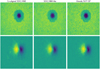 |
Fig. 1. Continuum intensity and the zonal component of the magnetic field for active region AR 11084, observed on 1 July 2010. Left: Co-aligned standard SDO/HMI observation. Middle: Degraded Hinode/SOT-SP observation. Right: Original Hinode/SOT-SP observation. The colour scales are the same within each row. |
4.3.1. PSF estimation
To estimate the HMI point-spread function, we selected quiet-Sun data from hmi.Ic_720s and hmi.Ic_720s_dconS observed at 19:00 UT on 5 May 2010. From the disk centre, we extracted a 401 × 401-pixel patch and flattened the continuum intensity using the polynomial surface fit. Since the noise contribution in continuum intensity images is negligible, the PSF was computed using the relation:
![Mathematical equation: $$ \begin{aligned} h(x, y) = \mathcal{F} ^{-1}\left[\frac{F(k_x, k_y)}{Z(k_x, k_y)}\right], \end{aligned} $$](/articles/aa/full_html/2025/05/aa53918-25/aa53918-25-eq26.gif) (16)
(16)
where F(kx, ky) and Z(kx, ky) represent the Fourier transforms of the hmi.Ic_720s and hmi.Ic_720s_dconS patches, respectively. For magnetic field measurements, the PSF can similarly be determined using active region data, where the noise – primarily related to the azimuth disambiguation – is minimal. Although the PSF derived from magnetic field data is consistent with that obtained from intensity maps, the latter allows for higher precision. Hence, we adopted the ‘intensity’ PSF to blur both the intensity and magnetic field vector datasets. The central part of the PSF is visualised in Fig. 2.
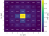 |
Fig. 2. Central part of the point-spread function computed from SDO/HMI surface granulation observations. |
4.3.2. Noise estimation
To estimate the noise contribution in the magnetic field vector, we analysed quiet-Sun regions observed at different times to isolate regions devoid of significant magnetic networks. Specifically, we used a patch observed at 19:00 UT on 5 May 2010, for the horizontal magnetic field, and another patch observed at 15:24 UT on 18 June 2010, for the radial magnetic field. These two separate observations were necessary to extract patches as large as possible while avoiding contamination from network magnetic fields. Specifically, the noise patch sizes in HMI-resolution pixels are 579 × 579, 635 × 635, and 81 × 81 for zonal, azimuthal, and radial field components respectively.
For each 72 × 72-pixel patch of blurred SOT-SP data, a noise component was generated to replicate the statistical properties of the original noise. This was done independently for each component of the magnetic field vector using the following procedure: First, the Fourier transform of the noise patches was computed, and low-frequency signals – potentially remnants of background magnetic fields – were filtered out. Second, a random phase distribution was applied, with symmetry enforced to ensure consistency with the Fourier transform of a real-valued signal. Third, the modified Fourier amplitudes and the random phases were transformed back to real space. Fourth, the HMI-pixel resolution noise was interpolated to the SOT-SP resolution and the central 72 × 72 pixels were cropped and added to the blurred SOT-SP observations. Since the Fourier amplitudes remained unchanged, this process ensured that the statistical properties of the original noise were preserved. By eliminating potential contamination from residual magnetic field signals, the generated noise closely mimics the properties of the original noise.
4.4. Observation filtering and splitting
In total, we collected 20 111 72 × 72 SOT-SP-resolution pixel patches. Even though we manually selected observations of active regions only, after cutting the data into final patches, most patches contained quiet-Sun regions surrounding the active regions. A quiet-Sun patch was defined as a patch of HMI-like data where the intensity was above 0.5 at all pixels, or where all components of the magnetic field were below 500 G. These patches were excluded from the dataset before model training. The remaining datum was split into training (70%), validation (20%), and test (10%) datasets. To avoid potential data leakage, the split was done chronologically, ensuring that similar images were not present in multiple parts. This approach minimises the risk of overfitting and ensures that the model performance is measured well. All data outside the date range of the training and validation datasets are also considered part of the test date range. Additionally, the quiet-Sun patches can be considered as test patches too but we distinguish the two in the following text. The patch counts for each quantity are summaries in Table 1.
Patch counts and date ranges in individual datasets.
5. Results
We built and trained a separate model for continuum intensity Ic, zonal magnetic field Bp, azimuthal magnetic field Bt, and radial magnetic field Br. The input data was the 72 × 72 SOT-SP-resolution pixel patches (i.e. approximately  in east-west and
  in south-north directions) of HMI-like observations. The targets were the corresponding 72 × 72-pixel patches of the SOT-SP observations. In figures, we follow the SOT-SP sign convention, namely Bp > 0 pointing west (towards the right), Bt > 0 pointing north (towards the top), and Br > 0 pointing away from the surface (against gravity).
5.1. Continuum intensity
Continuum intensity is the easiest to deconvolve because it contains little noise, which simplifies the deconvolution process. Additionally, there are no sign changes in the data, meaning that the information cannot be completely lost in low-resolution observations. We note that the RMSE values and absolute errors are in units normalised to quiet Sun, as described in Sect. 4.1.
In Fig. 3, we show the model error distribution in several ways. In the left panel, there is a log-density histogram together with overall metrics values. The red lines delimit certain error intervals. Most of the points follow the one-to-one dotted line with a steep decrease in density towards higher errors. The steep decrease is supported by the low overall RMSE and SAM metrics and by the high overall R2 metric. In the middle panel, there is a width of the error distribution from the left panel computed as the RMSE evaluated at specific bins. In this panel, we also plot the pixel count from which the RMSE was computed. A larger number of points causes the visible width increase around the quiet-Sun level, but the characteristic width of the error distribution is comparable in the whole intensity range, from the darkest umbra to the brightest centres of granules. The characteristic width is between 0.013 in umbrae to 0.025 in penumbrae and quiet Sun. The distribution of the worst predictions is visualised in the right panel. Taking into account the total pixel counts in the bins, the distribution of the worst pixels is nearly flat with a decrease in umbrae.
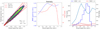 |
Fig. 3. Error evaluation of the intensity predictions. Left: Log-density plot of pixel-to-pixel correspondence between the actual and predicted values. The red lines delimit certain error levels. Middle: Error estimate of the predictions as a function of actual intensity (typical width of the distribution from the left panel). Right: The distribution of the worst predictions. The full lines show pixel counts while the dashed lines show the pixel densities. The dashed lines are in different colour shades for better visibility. |
In total, 97% of the pixels in the continuum intensity predictions exhibit absolute errors of 0.05 or lower (see Fig. 4 and Table 2). The remaining 3% are typically associated with abrupt intensity changes, often related to fine penumbral filaments that are imperfectly deconvolved, and also to discontinuities in the SOT-SP scans. Even though we removed the observations with well-visible discontinuities before the model training, the neural network model demonstrates the potential to identify additional corrupted observations. Notably, the model performs accurately outside the discontinuities, producing errors of approximately 0.1 along the discontinuities. We note that there are only 0.1% pixels with absolute error above 0.1.
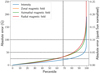 |
Fig. 4. Percentiles of the absolute errors between the predicted and target values. The horizontal dashed lines delimit 25 G, 50 G, and 100 G limits and 0.025, 0.05, and 0.1 quiet-Sun level limits. The vertical dashed line delimits the 1-σ estimate at 68.27 percentile. |
Fraction of data with an absolute error lower than the given limit.
The examples of the best and worst deconvolution results are plotted in Fig. 5. In general, the best results (top row) are in more homogeneous regions without high pixel-to-pixel intensity differences, such as quiet Sun, umbrae, pores, and even some parts of penumbrae. The highest error (bottom row) is typically associated with light bridges, umbral dots, or high-contrast fine penumbral filaments. Even in these cases, the model significantly improves the quality of the input images.
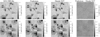 |
Fig. 5. Nine examples of individual intensity test patches. Left to right: Input data, model output, target output, model error. Top: Results with the lowest RMSE. Bottom: Results with the highest RMSE. The colour scales are the same for the first three panels within each row, while the right-most panel in each row has a distinct colour scale. |
The accuracy metrics computed from training, validation, test, and quiet-Sun datasets are all comparable, see Table 3. The similar accuracy metrics mean the model generalises well to new data. Potential improvement in the model accuracy can be achieved with a more complicated neural network model. To train such a model, one needs to collect more data to constrain more model parameters. We note that the error of the presented model is small and the improvement due to the larger model will likely be negligible compared to the increase in model training time and memory consumption.
Overall evaluation of accuracy metrics for all four datasets.
5.2. Horizontal magnetic field
Unlike continuum intensity, the magnetic field can exhibit sign changes that complicate deconvolution and may result in the loss of important details. This is especially relevant for the horizontal field, where abrupt changes in the field direction are more frequently localised in small unresolved areas.
The detailed statistical information about the model predictions is plotted in Fig. 6. In models of both components, we can see similar trends. As shown in the log-density plots (left panels), the models are accurate in strong horizontal field regions, but there is a significant scatter if the field amplitude is below 300 G. The dominant source of the low-field scatter is azimuth disambiguation in quiet-Sun regions. This is associated with disambiguation noise whose amplitude can reach up to 300 G. The standard deviation of the disambiguation noise in the input data is approximately 58 G and 64 G for the zonal and azimuthal components, respectively. The overall RMSE metric of both components is about 40 G. The widths of the distributions (middle panels) indicate that the model error remains below 50 G for magnetic field strengths up to 1000 G and below 100 G for stronger fields. Notably, 75% of the target pixels are located in regions where the field amplitude is under 300 G, dominated by disambiguation noise. The overall RMSE, as well as the RMSE within bins for field amplitudes below 1000 G, is substantially lower than the standard deviation of the disambiguation noise. This demonstrates that the model effectively deconvolves real signals, not merely ignoring the noise but actively suppressing it. In the original SOT-SP observations, two types of disambiguation noise are present: random and chess-like. In the chess-like noise, the sign alternates periodically between neighbouring pixels. These sign changes are removed from the input HMI-like data after the convolution with the HMI PSF and are not restored by the model. In such cases, the model predictions are rather a correction to the original data. For bins corresponding to very strong fields above 2000 G, the RMSE often exceeds 100 G, which is approximately 5% of the field strength. These bins represent a small fraction of the dataset (0.01%) and thus present challenges for model training due to limited data availability. The distributions of predictions with RMSE > 50 G and RMSE > 100 G are shown in the right panels. The prediction errors for the horizontal magnetic field are primarily attributed to disambiguation noise. In regions where the unsigned horizontal field is below 300 G, 85% (zonal) and 89% (azimuthal) of points with model errors exceeding 100 G are found. Furthermore, the density of erroneous pixels is notably higher in these regions compared to regions with stronger fields.
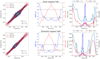 |
Fig. 6. Error evaluation of the predictions of the horizontal magnetic field. Top: Zonal component. Bottom: Azimuthal component. Left: Log-density plot of pixel-to-pixel correspondence between the actual and predicted values. The red lines delimit certain error levels. Middle: Error estimate of the predictions as a function of actual field amplitude (typical width of the distribution from the left panel). Right: The distribution of the worst predictions. The full lines show pixel counts while the dashed lines show the pixel densities. The dashed lines are in different colour shades for better visibility. |
In total, the model predictions for the two horizontal magnetic field components are comparable, with approximately 84% of predictions within an absolute error of 50 G and over 97% within 100 G (see Fig. 4 and Table 2). In areas with strong magnetic fields, the error sources are similar to those identified for continuum intensity predictions. These include sharp boundaries caused by observational discontinuities and incorrect field measurements in the target data, such as isolated low-amplitude pixels surrounded by a high-amplitude region.
Nine examples of both the best (top rows) and the worst (bottom rows) deconvolved images are shown in Figs. 7 and 8. As in the previous, we can observe similar structures here. The best deconvolution results were typically computed for ‘single-sign’ input images with amplitudes lower than 1.5 kG. The worst results were observed in areas affected by the chess-like noise, which is visible in almost all panels (several of these regions are highlighted with the red boxes in Fig. 7, requiring zoom for better visibility), regions with abrupt sign changes (highlighted by the blue box in Fig. 7), or misaligned SOT-SP scans (highlighted by the red box in Fig. 8). In the maps, one can also see how the model deals with disambiguation noise. The best example is the middle-right panel in the top row in Fig. 7. There, in the top-left corner is part of the penumbra that is deconvolved with minimum artefacts. All other parts are dominated by the disambiguation noise. The random nature of the noise created a small but coherent pore-like feature, highlighted by the yellow boxes, just below the penumbra, close to the horizontal centre. This feature was considered real and was restored by the model, while other areas dominated by the noise were efficiently denoised. As the feature is due to noise, it is not present in the original SOT-SP image and is well-visible in the right-most column of Fig. 7.
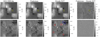 |
Fig. 7. Nine examples of individual zonal field test patches. Left to right: Input data, model output, target output, model error. Top: Results with the lowest RMSE. Bottom: Results with the highest RMSE. The colour scales are the same for the first three panels within each row, while the right-most panel in each row has a distinct colour scale. The pore-like structure is marked by the yellow boxes, the chess-like noise is highlighted by the red boxes, and the abrupt sign changes are indicated by the blue box. |
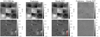 |
Fig. 8. Nine examples of individual azimuthal field test patches. Left to right: Input data, model output, target output, model error. Top: Results with the lowest RMSE. Bottom: Results with the highest RMSE. The colour scales are the same for the first three panels within each row, while the right-most panel in each row has a distinct colour scale. The misaligned SOT-SP scans are highlighted by the red box. |
The accuracy metrics are summarised in Table 3. Unlike the quiet-Sun patches, the training, validation, and test datasets are statistically similar. The similar metric values for these datasets show the model is not overfitted and generalises well to new data. The metrics for the quiet-Sun patches are affected by the limited magnetic field range. At first glance, it is surprising that RMSE for the quiet-Sun dataset is the lowest, even though these patches are dominated by noise. However, the low RMSE values are not indicative of better deconvolution but are instead related to the limited amplitude of the magnetic field in this dataset, which inherently reduces absolute errors. Despite this, the relative errors are higher, as reflected in the significantly worse R2 and SAM metrics, which highlight the high scatter in prediction–actual space.
5.3. Radial magnetic field
The deconvolution of the radial magnetic field deals with less noise in input data compared to the horizontal magnetic field and also the abrupt sign changes are mostly related to the lessfrequent complex topology of magnetic field lines.
The model prediction statistics are plotted in Fig. 9. The log-density histogram in the left panel shows a very good deconvolution in quiet-Sun regions and regions of the field stronger than about 1000 G. In the intermediate field strength, the histogram width increases. This increase cannot be explained by the noise, whose amplitude is up to 300 G only. The larger scatter causes an increase in the overall RMSE to 44 G. The middle panel shows the increase in the histogram width. The two peaks are symmetric and the error is above 65 G for field unsigned amplitude between 350 G and 750 G, both peaks have a maximum at 550 G. The histogram of the worst predictions is visualised in the right panel. Most of the high-error points are in regions of almost 0 G amplitude. This is attributed to the high number of data points there–the density of the high-error points is relatively low. Unlike in the case of the horizontal field, the histogram shows a significant number of high-error pixels up to 1500 G. The highest high-error pixel density is around 500 G, which corresponds to the results from the middle panel.
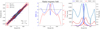 |
Fig. 9. Error evaluation of the predictions of the radial magnetic field. Left: Log-density plot of pixel-to-pixel correspondence between the actual and predicted values. The red lines delimit certain error levels. Middle: Error estimate of the predictions as a function of actual field amplitude (typical width of the distribution from the left panel). Right: The distribution of the worst predictions. The full lines show pixel counts while the dashed lines show the pixel densities. The dashed lines are in different colour shades for better visibility. |
In total, 82% and 96% of pixels have error below 50 G and 100 G, respectively (see Fig. 4 and Table 2). In strong magnetic fields, the highest error appears at sharp boundaries and in neighbouring bipolar regions. In the mid-amplitude field regions, yet the source of the error in model predictions is unknown.
The top and bottom rows of Fig. 10 illustrate the best and worst deconvolution results, respectively. The most accurate reconstructions are predominantly observed in quiet-Sun regions with small-scale magnetic fields. Even in areas where the noise amplitude is comparable to the signal (highlighted by the yellow boxes), the fine details of the field are well reconstructed. These nine patches also highlight the original noise present in the radial component of the HMI data and demonstrate how it was effectively minimised in the deconvolved images. The reconstructions with the highest RMSE are shown in the bottom row. These regions exhibit complex field topologies where the radial field direction frequently changes. Despite these challenges, the modelled images closely match the target ones, with noticeable differences only at the smallest scales. This is true even for small-amplitude structures at the level of background noise (highlighted by the red and blue boxes), which the model successfully distinguished from noise and deconvolved with precision.
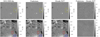 |
Fig. 10. Nine examples of individual radial field test patches. Left to right: Input data, model output, target output, model error. Top: Results with the lowest RMSE. Bottom: Results with the highest RMSE. The colour scales are the same for the first three panels within each row, while the right-most panel in each row has a distinct colour scale. The successful reconstruction of structures dominated by noise is marked by the yellow, red, and blue boxes. |
The accuracy metrics for the radial magnetic field are listed in Table 3. As with the horizontal field, the training, validation, and test datasets are consistent, indicating that the model is not overfitted and generalises well to new data. The lower RMSE for the quiet-Sun patches gives a misleading impression of better performance, primarily due to the lower magnetic field amplitudes in these regions, which reduce absolute errors. However, the R2 and SAM metrics provide a more accurate picture, highlighting the deterioration of model predictions in the quiet-Sun regions, where the relative errors are higher despite the lower RMSE.
6. Discussion
The performance of complex neural network models is inherently related to the quality of the training data. Biases present in the data are learned by the model, potentially degrading its performance. Furthermore, the model itself incorporates assumptions about the data, which are typically not fully under control. In our case, the training utilises HMI-like data, whereas the model is designed to operate on actual HMI observations. Discrepancies between these two datasets introduce additional biases that can affect the model’s effectiveness.
6.1. Biases
The input training data are non-uniformly distributed. To improve the model predictions, we modified the MSE loss function to emphasise sparsely populated data while minimally affecting densely populated data. The loss function ℒ used and the weighted factors w have the form:
![Mathematical equation: $$ \begin{aligned} \mathcal{L}&= \sum \limits _i \left[\boldsymbol{w}_i \left( \text{ actual}_i - \text{ predicted}_i\right)^2 \right], \end{aligned} $$](/articles/aa/full_html/2025/05/aa53918-25/aa53918-25-eq29.gif) (17)
(17)
![Mathematical equation: $$ \begin{aligned} \boldsymbol{w}&= \max \left[ \log \left( \mu \frac{N}{\boldsymbol{n}} \right),\ \boldsymbol{1} \right], \end{aligned} $$](/articles/aa/full_html/2025/05/aa53918-25/aa53918-25-eq30.gif) (18)
(18)
where i counts the individual patches, n is the vector representing the number of data points in each bin, N is the total number of data points, and μ is a free parameter set to 0.15. The bin widths were selected as 0.05 and 50 G for intensity and magnetic field, respectively. If the number of points in a bin exceeds μ/e ≈ 5.5% of the total points, these points are not emphasised by the weights. The original and adjusted distributions are visualised in Fig. 11. The original distribution is represented by the black bar contours, while the adjusted distribution is shown using the blue bars.
 |
Fig. 11. Distribution of input training data. The black bar contours represent the original distribution and the blue bars the corrected distribution. |
Although the weighted distribution is non-uniform, no systematic errors–computed as the mean difference between predicted and actual values of the test data in each specific bin–are observed in well-populated bins where such errors are well-defined. This holds for intensities below 1.2 times the quiet-Sun level, horizontal fields below 2 kG, and radial fields below 3 kG. The systematic errors computed from the test dataset are illustrated in Fig. 12. Therefore, we conclude that the biases due to the input data are negligible in most real situations.
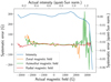 |
Fig. 12. Systematic errors computed in small bins of the test dataset. In well-populated bins, the systematic error is negligible. |
To perform deconvolution, we employ convolutional neural networks. Numerical convolution requires the specification of boundary conditions. Two commonly used options are ‘no padding’ and ‘zero padding’. No padding reduces the image size, making it unsuitable for our purposes. On the other hand, zero padding assumes low data values near the image edges, which is inconsistent with our data. Following Díaz Baso & Asensio Ramos (2018), we opted for reflection boundary conditions, which assume coherent structures at the boundaries. While this approach is the most suitable for HMI observations, it is not entirely ideal. To minimise the impact of boundary effects, which in our case influence 10 pixels on each side, we selected relatively large 72 × 72-pixel patches for training. The RMSE values calculated from the central 52 × 52 pixels of the test data are 0.0216, 39.2 G, 38.9 G, and 42.6 G for intensity, zonal field, azimuthal field, and radial field, respectively. These values are lower than those reported in Table 3, but the differences are negligible. We note that the metrics values stabilise if only 2 pixels from each side are cut. This demonstrates that reflection boundary conditions perform well and introduce minimal bias during model training. We note that in the evaluation of the trained model, users can input a larger image and cut the edges of the predicted output.
6.2. Reliability of the HMI-like dataset
The key assumption of our model is that the HMI-like dataset is equivalent to the actual HMI dataset. To test this assumption, we needed to test three aspects of the data: 1) Is the PSF precise enough? 2) Are the noise statistics correctly computed? 3) Does the deconvolution of actual HMI data create artefacts?
6.2.1. Point-spread function
The PSF was computed directly from the standard and deconvolved HMI intensity observations. We demonstrate the similarity of HMI and HMI-like observations on the patches visualised in Fig. 1. The pixel value densities are shown in Fig. 13. The HMI and HMI-like distributions are comparable. They differ in regions close to 0.8 intensity, where the penumbra contributes to the pixel density. The discrepancy may be caused by multiple interpolations that were performed to align HMI and SOT-SP observations. Another contribution is due to the difference in observation time, and therefore different granulation patterns. We compared the overall sharpness metrics from the quiet Sun in Fig. 1. The results are summarised in Table 4. The small difference between the actual and simulated HMI observation can be attributed to the differences in granulation patterns. We conclude that the computed PSF is most likely very close to the exact HMI PSF.
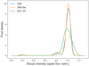 |
Fig. 13. Density kernel plot computed from intensity plotted in Fig. 1. The HMI and HMI-like distributions are comparable except for the penumbra region, which is close to 0.8 intensity. This may be due to multiple interpolations of the HMI observations during its alignment with SOT-SP observations. |
The PSF was further computed from individual patches of the data and compared to the final PSF. The patches were selected using a sliding window approach, with each patch measuring 401 × 401 pixels and extracted with a stride of 66 pixels in both directions, resulting in a total of 1916 patches fully covered by the solar disk. Despite the expected influence of limb darkening and projection effects, the differences were remarkably small across the majority of the patches. Only 11 patches exhibited a maximum unsigned difference exceeding 0.05 between the patch-derived PSF and the final PSF. Notably, the maximum differences above 0.05 were always observed in the central pixel of the PSF. This consistency indicates that the computed PSF is robust and accurately represents the HMI observations across the whole disk. The HMI observation, the central patch from which the PSF was computed (black), and the locations of the outlier patches (dashed red) are shown in Fig. 14. These patches were primarily located near the solar limb, yet most of the limb regions showed sufficient agreement. Furthermore, the central patch is very close to one of the outlier patches, which has a difference of 0.07. This suggests that a difference of 0.07 may represent the variability or ‘realisation noise’ in the central pixel of the PSF.
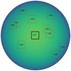 |
Fig. 14. HMI continuum intensity observation at 19:00 UT on 5 May 2010. The red dashed patches outline regions where the computed PSF and the applied PSF differ by more than 0.05 in maximum unsigned value. Numerical values within the patches indicate the differences. The black patch shows the regions where the applied PSF was computed. |
The same PSF is used for all SOT-SP observations. If long-term changes in the HMI PSF are present, they could degrade the model’s performance. To assess this, we analysed long-term variations in real HMI data by selecting quiet-Sun disk-centre observations from 1 July each year between 2010 and 2023. First, we computed the PSF from these data and compared it with the PSF used to blur SOT-SP observations. The maximum absolute difference between the PSFs and the used PSF is below 0.02 which is much lower than the expected realisation noise. Moreover, there is no trend with time and the maximum difference oscillates around 0.01. Second, we deconvolved the HMI data and evaluated the consistency of the model output over time. The granulation contrast is 6.3%±0.2 pp with a maximum difference of 0.5 pp. We note that the original HMI datum has contrast 2.7%±0.7 pp. These results indicate that potential long-term changes in the HMI PSF do not significantly affect the deconvolution performance of the model.
6.2.2. Noise realisation
The noise patterns were selected from quiet-Sun regions of SDO/HMI observation with minimal background magnetic field to provide a clean reference. We performed a Fourier analysis on these noise patterns and filtered out low-frequency contributions, specifically frequencies lower than 4% of the Nyquist frequency. The frequency amplitudes were then inverted using symmetrised random phases to produce a real-space noise realisation. This approach effectively utilises the full amplitude information, corresponding to the complete covariance matrix, while being computationally efficient in terms of time and memory. However, it has a significant limitation: the method inherently assumes periodic boundary conditions, which are not valid for the noise.
To mitigate the effects of periodic boundary conditions, we generated a noise field larger than the desired 72 × 72-pixel patches. By cropping the central 72 × 72-pixel region from the larger noise field, we minimised the influence of edge artefacts caused by the periodic assumption. Then, this cropped noise patch was added to the corresponding data patch. The specific noise pattern is particularly important for the horizontal magnetic field components, where disambiguation noise dominates the signal in the quiet Sun. For these components, the full-size noise patterns in the final SOT-SP pixel size extend to 983 × 913 pixels for the zonal component and 1078 × 1001 pixels for the azimuthal component, both in format east-west × south-north directions. This scale ensures that the invalidity of the periodic boundary conditions has minimal impact on the central regions of the cropped noise patches, which are added to the data. Finding the no-field noise patch for the radial component is a difficult task and the resulting patch size is 137 × 128 SOT-SP-resolution pixels. This size still ensures that the periodic boundary conditions play no significant role in the central part of the generated noise. Moreover, the highest sensitivity of the central patches to the boundary conditions comes from the low-frequency (i.e. long-range) terms in Fourier space that were filtered out.
We conducted experiments with training data featuring different noise statistics to explore the amplification of noise during the deconvolution of actual SDO/HMI observations. Although neural networks incorporate implicit noise regularisation (see the last paragraph of Sect. 3.1), the predictions still exhibit amplified disambiguation noise when the noise characteristics differ between the training and evaluation datasets. Fig. 15 illustrates this effect with predictions on SDO/HMI data observed on 1 July 2010, under extreme conditions. The left panel shows the original observation, the middle panel presents the model prediction when trained without the noise component, and the right panel displays the prediction that incorporates the correct noise statistics. These comparisons highlight the sensitivity of deconvolution performance to accurate noise modelling during training. Interestingly, when artificial noise that was visually similar but statistically different from the actual noise was added to the training data, the resulting deconvolution showed only a slight improvement over the middle panel of Fig. 15. This result underscores the importance of incorporating statistically accurate noise in the training process. Additionally, it offers a reliable method for assessing the quality of the artificial noise introduced.
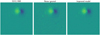 |
Fig. 15. Zonal magnetic field for active region AR 11084, observed on 1 July 2010 with SDO/HMI, alongside deconvolution results using two models: one with incorrect noise statistics and the other with correct noise statistics. The colour scales are the same. |
6.2.3. Actual HMI deconvolution
The final test of the PSF and noise realisations was conducted using HMI observations of active region AR 12797 at 12:00 UT on 23 January 2021. This date forms part of the test dataset for all four deconvolved quantities. The HMI observations were deconvolved by the neural network model, and these images were subsequently compared with the corresponding HMI_dconS images. All observations of the active region are presented in Fig. 16.
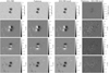 |
Fig. 16. Comparison of the HMI deconvolution pipeline and CNN-based modelled deconvolution. Top to bottom: Intensity, zonal magnetic field, azimuthal magnetic field, and radial magnetic field. Left to right: SDO/HMI observations of active region AR 12797 at 12:00 UT on 23 January 2021, CNN-deconvolved results, HMI_dconS-deconvolved results, and the difference between the CNN and HMI_dconS deconvolution results. The colour scales are the same for the first three panels within each row, while the right-most panel in each row has a distinct colour scale. |
The model predictions show notable improvements over HMI_dconS images across all components, with the most significant enhancements observed in the intensity and radial field panels. In the intensity panels, the granulation pattern in the difference column (right-most column) forms an ‘inverse’ web, characterised by negative-value lines surrounding positive-value centres. This pattern arises because subtracting a blurred [baseline=(current bounding box.south)] (0,0) – (0.15,0) – (0.15,0.2) – (0.35,0.2) – (0.35,0) – (0.5,0); -like edge (HMI_dconS) from a sharp edge (model prediction) produces negative values along the sides and positive values in the centre. For the zonal and azimuthal magnetic field components, the predictions show significantly reduced disambiguation noise and exhibit much sharper field structures. Additionally, the neural network demonstrates an ability to resolve fine-scale features and recover spatially coherent low-field structures when these are sufficiently large. In the radial field panels, the model’s predictions display a much sharper and clearer magnetic field. The neural network effectively reduces noise in quiet-Sun regions, allowing for the reconstruction of subtle spatial structures that would otherwise remain hidden. This includes the intricate quiet-Sun magnetic network as well as enhanced detail in stronger fields within the inner penumbra and umbra. The model also improves the resolution of low-field regions that were nearly hidden in noise, provided these structures span several spatially coherent pixels. Across all magnetic field components, the model predictions enhance spatially coherent structures while effectively suppressing random noise, leading to sharper, cleaner, and more accurate representations of the underlying solar magnetic field.
The image sharpness metrics, evaluated at the quiet Sun disk centre, are provided in Table 5, showing significant improvements across all metrics compared to the HMI_dconS observations. Notably, the granulation contrast of the CNN-deconvolved results is close to the value of 6.8% measured previously with SOT-SP. Additionally, the gradient magnitude metric, which is only linearly dependent on pixel size, shows only a small difference between the CNN model and SOT-SP. In contrast, Laplacian variance depends strongly on the pixel size, which varies with the position of the observation on the solar disk. As a result, direct comparisons with Table 4 can be challenging. The improvements in metrics highlight the superior resolution and precision achieved by the model compared to the HMI_dconS deconvolution and support the explanation of the inverse web pattern discussed earlier.
Neither the model’s output nor HMI_dconS shows obvious deconvolution artefacts, even in regions with complex magnetic field structures, such as in Fig. 16. The absence of such artefacts indicates that the computed PSF closely approximates the true PSF. In comparison, HMI_dconS can exhibit strong artefacts, particularly in regions of strong magnetic fields. This issue was evident when we tested it on data from active region AR 11084, visualised in Fig. 1, where HMI_dconS produced artefacts with opposite signs of radial field in the umbral centre. The model, however, does not introduce these artefacts, as they are not present in the original HMI data. Additionally, the relatively blurry nature of the HMI_dconS results naturally reduces the occurrence of artefacts, whereas the NN model preserves sharpness without introducing artefacts, even in complex or strong fields. Furthermore, unlike the HMI_dconS maps, the CNN-based deconvolution reduces noise in the horizontal field maps, whereas noise levels remain largely unchanged in the HMI_dconS images. This highlights that the noise incorporated into the training data closely mirrors the noise in the HMI observations, and the CNN model successfully learns to deconvolve the signal while suppressing the noise present in the HMI data.
7. Conclusions
We trained a convolutional neural network model to perform the deconvolution of intensity and vector magnetic field observations from SDO/HMI. For training, we used Hinode/SOT-SP data and simulated SDO/HMI-like observations, where the simulations incorporated the Hinode/SOT-SP observations and exact SDO/HMI point-spread function and noise statistics. Our results demonstrate that the model effectively distinguishes between signal and noise, applying deconvolution only to the signal. Crucially, the use of accurate noise statistics was essential for achieving successful deconvolution in the quiet Sun, where noise dominates the low-amplitude magnetic field, particularly in the horizontal field components. The model can deconvolve coherent structures even in these challenging conditions. The deconvolved output achieved by the model retains the same level of detail as the Hinode observations. Furthermore, the model outperforms the existing deconvolution products from the HMI pipeline. The model is applicable to any image size, including full-disk observations, ensuring scalability across a range of datasets. However, due to boundary conditions, the minimum required size for processing is 40 × 40 Hinode-resolution pixels, that is a size of 68″ × 63″ in longitude × latitude.
Acknowledgments
This research is supported by the Czech–German common grant, funded by the Czech Science Foundation under the project 23-07633K and by the Deutsche Forschungsgemeinschaft under the project BE 5771/3-1 (eBer-23 13412) and the institutional support RVO:67985815. This research has made use of NASA’s Astrophysics Data System Bibliographic Services. The authors would like to thank the anonymous referee for their valuable comments and suggestions that greatly improved the quality of the paper.
References
- Abadi, M., Agarwal, A., Barham, P., et al. 2015, TensorFlow: Large-Scale Machine Learning on Heterogeneous Systems, software available from tensorflow.org [Google Scholar]
- Chollet, F., et al. 2015, Keras https://keras.io [Google Scholar]
- Díaz Baso, C. J., & Asensio Ramos, A. 2018, A&A, 614, A5 [NASA ADS] [CrossRef] [EDP Sciences] [Google Scholar]
- Goodfellow, I., Bengio, Y., & Courville, A. 2016, Deep Learning (MIT Press), https://www.deeplearningbook.org [Google Scholar]
- Hapgood, M. A., Dimbylow, T. G., Sutcliffe, D. C., et al. 1997, Space Sci. Rev., 79, 487 [Google Scholar]
- Hoeksema, J. T., Liu, Y., Hayashi, K., et al. 2014, Sol. Phys., 289, 3483 [Google Scholar]
- Jarolim, R., Thalmann, J. K., Veronig, A. M., & Podladchikova, T. 2023, Nat. Astron., 7, 1171 [NASA ADS] [CrossRef] [Google Scholar]
- Kelley, H. J. 1960, ARS J., 30, 947 [Google Scholar]
- Kingma, D. P., & Ba, J. 2014, ArXiv e-prints [arXiv:1412.6980] https://www.researchgate.net/publication/269935079_Adam_A_Method_for_Stochastic_Optimization [Google Scholar]
- Kosugi, T., Matsuzaki, K., Sakao, T., et al. 2007, Sol. Phys., 243, 3 [Google Scholar]
- Leka, K. D., Barnes, G., & Crouch, A. 2009, in The Second Hinode Science Meeting: Beyond Discovery-Toward Understanding, eds. B. Lites, M. Cheung, T. Magara, J. Mariska, & K. Reeves, ASP Conf. Ser., 415, 365 [Google Scholar]
- Lites, B., Casini, R., Garcia, J., & Socas-Navarro, H. 2007, Mem. Soc. Astron. It., 78, 148 [NASA ADS] [Google Scholar]
- Lites, B. W., Akin, D. L., Card, G., et al. 2013, Sol. Phys., 283, 579 [NASA ADS] [CrossRef] [Google Scholar]
- Lucy, L. B. 1974, AJ, 79, 745 [Google Scholar]
- Norton, A. A., Duvall, T., Schou, J., Cheung, M., & Scherrer, P. H. 2017, in AAS/Solar Physics Division Abstracts. 48, 207.05 [Google Scholar]
- Norton, A. A., Duvall, T. L., Jr., Schou, J., et al. 2018, Catalyzing Solar Connections, 101 [Google Scholar]
- Penttilä, A., Hietala, H., & Muinonen, K. 2021, A&A, 649, A46 [NASA ADS] [CrossRef] [EDP Sciences] [Google Scholar]
- Pesnell, W. D., Thompson, B. J., & Chamberlin, P. C. 2012, Sol. Phys., 275, 3 [Google Scholar]
- Rahman, S., Moon, Y.-J., Park, E., et al. 2020, ApJ, 897, L32 [NASA ADS] [CrossRef] [Google Scholar]
- Richardson, W. H. 1972, J. Opt. Soc. Am. (1917–1983), 62, 55 [Google Scholar]
- Scherrer, P. H., Schou, J., Bush, R. I., et al. 2012, Sol. Phys., 275, 207 [Google Scholar]
- Schou, J., Scherrer, P. H., Bush, R. I., et al. 2012, Sol. Phys., 275, 229 [Google Scholar]
- Tsuneta, S., Ichimoto, K., Katsukawa, Y., et al. 2008, Sol. Phys., 249, 167 [Google Scholar]
- Valizadegan, H., Martinho, M. J. S., Wilkens, L. S., et al. 2022, ApJ, 926, 120 [NASA ADS] [CrossRef] [Google Scholar]
- Wang, R., Fouhey, D. F., Higgins, R. E. L., et al. 2024, ApJ, 970, 168 [Google Scholar]
- Wiener, N. 1949, Extrapolation, Interpolation, and Smoothing of Stationary Time Series: with Engineering Applications (The MIT press) [CrossRef] [Google Scholar]
All Tables
All Figures
|
Fig. 1. Continuum intensity and the zonal component of the magnetic field for active region AR 11084, observed on 1 July 2010. Left: Co-aligned standard SDO/HMI observation. Middle: Degraded Hinode/SOT-SP observation. Right: Original Hinode/SOT-SP observation. The colour scales are the same within each row. |
| In the text | |
|
Fig. 2. Central part of the point-spread function computed from SDO/HMI surface granulation observations. |
| In the text | |
|
Fig. 3. Error evaluation of the intensity predictions. Left: Log-density plot of pixel-to-pixel correspondence between the actual and predicted values. The red lines delimit certain error levels. Middle: Error estimate of the predictions as a function of actual intensity (typical width of the distribution from the left panel). Right: The distribution of the worst predictions. The full lines show pixel counts while the dashed lines show the pixel densities. The dashed lines are in different colour shades for better visibility. |
| In the text | |
|
Fig. 4. Percentiles of the absolute errors between the predicted and target values. The horizontal dashed lines delimit 25 G, 50 G, and 100 G limits and 0.025, 0.05, and 0.1 quiet-Sun level limits. The vertical dashed line delimits the 1-σ estimate at 68.27 percentile. |
| In the text | |
|
Fig. 5. Nine examples of individual intensity test patches. Left to right: Input data, model output, target output, model error. Top: Results with the lowest RMSE. Bottom: Results with the highest RMSE. The colour scales are the same for the first three panels within each row, while the right-most panel in each row has a distinct colour scale. |
| In the text | |
|
Fig. 6. Error evaluation of the predictions of the horizontal magnetic field. Top: Zonal component. Bottom: Azimuthal component. Left: Log-density plot of pixel-to-pixel correspondence between the actual and predicted values. The red lines delimit certain error levels. Middle: Error estimate of the predictions as a function of actual field amplitude (typical width of the distribution from the left panel). Right: The distribution of the worst predictions. The full lines show pixel counts while the dashed lines show the pixel densities. The dashed lines are in different colour shades for better visibility. |
| In the text | |
|
Fig. 7. Nine examples of individual zonal field test patches. Left to right: Input data, model output, target output, model error. Top: Results with the lowest RMSE. Bottom: Results with the highest RMSE. The colour scales are the same for the first three panels within each row, while the right-most panel in each row has a distinct colour scale. The pore-like structure is marked by the yellow boxes, the chess-like noise is highlighted by the red boxes, and the abrupt sign changes are indicated by the blue box. |
| In the text | |
|
Fig. 8. Nine examples of individual azimuthal field test patches. Left to right: Input data, model output, target output, model error. Top: Results with the lowest RMSE. Bottom: Results with the highest RMSE. The colour scales are the same for the first three panels within each row, while the right-most panel in each row has a distinct colour scale. The misaligned SOT-SP scans are highlighted by the red box. |
| In the text | |
|
Fig. 9. Error evaluation of the predictions of the radial magnetic field. Left: Log-density plot of pixel-to-pixel correspondence between the actual and predicted values. The red lines delimit certain error levels. Middle: Error estimate of the predictions as a function of actual field amplitude (typical width of the distribution from the left panel). Right: The distribution of the worst predictions. The full lines show pixel counts while the dashed lines show the pixel densities. The dashed lines are in different colour shades for better visibility. |
| In the text | |
|
Fig. 10. Nine examples of individual radial field test patches. Left to right: Input data, model output, target output, model error. Top: Results with the lowest RMSE. Bottom: Results with the highest RMSE. The colour scales are the same for the first three panels within each row, while the right-most panel in each row has a distinct colour scale. The successful reconstruction of structures dominated by noise is marked by the yellow, red, and blue boxes. |
| In the text | |
|
Fig. 11. Distribution of input training data. The black bar contours represent the original distribution and the blue bars the corrected distribution. |
| In the text | |
|
Fig. 12. Systematic errors computed in small bins of the test dataset. In well-populated bins, the systematic error is negligible. |
| In the text | |
|
Fig. 13. Density kernel plot computed from intensity plotted in Fig. 1. The HMI and HMI-like distributions are comparable except for the penumbra region, which is close to 0.8 intensity. This may be due to multiple interpolations of the HMI observations during its alignment with SOT-SP observations. |
| In the text | |
|
Fig. 14. HMI continuum intensity observation at 19:00 UT on 5 May 2010. The red dashed patches outline regions where the computed PSF and the applied PSF differ by more than 0.05 in maximum unsigned value. Numerical values within the patches indicate the differences. The black patch shows the regions where the applied PSF was computed. |
| In the text | |
|
Fig. 15. Zonal magnetic field for active region AR 11084, observed on 1 July 2010 with SDO/HMI, alongside deconvolution results using two models: one with incorrect noise statistics and the other with correct noise statistics. The colour scales are the same. |
| In the text | |
|
Fig. 16. Comparison of the HMI deconvolution pipeline and CNN-based modelled deconvolution. Top to bottom: Intensity, zonal magnetic field, azimuthal magnetic field, and radial magnetic field. Left to right: SDO/HMI observations of active region AR 12797 at 12:00 UT on 23 January 2021, CNN-deconvolved results, HMI_dconS-deconvolved results, and the difference between the CNN and HMI_dconS deconvolution results. The colour scales are the same for the first three panels within each row, while the right-most panel in each row has a distinct colour scale. |
| In the text | |
Current usage metrics show cumulative count of Article Views (full-text article views including HTML views, PDF and ePub downloads, according to the available data) and Abstracts Views on Vision4Press platform.
Data correspond to usage on the plateform after 2015. The current usage metrics is available 48-96 hours after online publication and is updated daily on week days.
Initial download of the metrics may take a while.