| Issue |
A&A
Volume 664, August 2022
|
|
|---|---|---|
| Article Number | A152 | |
| Number of page(s) | 7 | |
| Section | Numerical methods and codes | |
| DOI | https://doi.org/10.1051/0004-6361/202243812 | |
| Published online | 25 August 2022 | |
Aspects of thermal modeling using digital terrain models
Assessing indirect radiation, the solar limb darkening effect, and depth profiles: Application to Mercury’s north polar MLA DTM
1
Technische Universität Berlin, Institute of Geodesy and Geoinformation Science,
Kaiserin-Augusta-Allee 104-106,
10553
Berlin, Germany
e-mail: philipp.glaeser@tu-berlin.de
2
Ronin Institute for Independent Scholarship,
Montclair,
07043
New Jersey, USA
Received:
19
April
2022
Accepted:
20
June
2022
Context. Our thermal model is adapted and extended in this study. Specifically the aspect of handling indirect radiation, the solar limb darkening effect, and depth profiles are addressed.
Aims. Our goal is to improve the existing thermal model to handle terrain scattering and re-radiation in an adaptive way. In addition, we aim to change previously fixed and manually chosen discretization of the solar limb darkening effect and depth profile to be adaptive and applicable for various planets and purposes.
Methods. The temperature was modeled based on digital terrain models (DTMs) using data of the Mercury Laser Altimeter (MLA). New implementations to handle terrain scattering and re-radiation were introduced using level-of-detail techniques. The solar disk was discretized into a variable number of rings and the depth profile was introduced as an exponential function for which the number of nodes and the maximum depth can be chosen.
Results. We present results for the ideal window size and degree of level-of-detail for thermal studies of the Hermean north pole. Further we show that the previous discretization of the solar limb darkening effect proved insufficient for Mercury, and we updated the implementation accordingly. Similarly we improved the implementation for the depth profile. For the first time, we derived depth-to-ice, as well as average and maximum temperature maps based on thermal modeling of the complete north polar MLA DTM.
Key words: radiation mechanisms: thermal / methods: numerical / planets and satellites: surfaces
© P. Gläser 2022
 Open Access article, published by EDP Sciences, under the terms of the Creative Commons Attribution License (https://creativecommons.org/licenses/by/4.0), which permits unrestricted use, distribution, and reproduction in any medium, provided the original work is properly cited.
This article is published in open access under the Subscribe-to-Open model. Subscribe to A&A to support open access publication.
1 Introduction
Despite being the closest planet to the Sun with high daytime surface temperatures, the possibility of water ice accumulating in Mercury’s polar regions was still debated (Thomas 1974). Similar studies at the lunar poles have postulated that water ice could accumulate in so-called permanently shadowed regions (PSRs) (Watson et al. 1961; Arnold 1979). PSRs usually emerge in near-polar crater floors. Here, the crater interiors are shielded from direct sunlight due to the near-zero tilt of the Hermean (or lunar) rotational axis with respect to the ecliptic plane in interaction with the topography in its vicinity. As a result, the crater floors remain in permanent darkness with stable and cold temperatures allowing for water ice to accumulate.
Radar observations of Mercury’s poles revealed extensive areas of radar bright deposits (Slade et al. 1992; Harmon & Slade 1992; Harmon et al. 2011). Those observations are consistent with water ice (Vasavada et al. 1999; Harmon et al. 2011; Paige et al. 2013) and the deposits were found to be located inside PSRs. Paige et al. (1992) used thermal modeling techniques to derive temperatures for various idealized surfaces such as flat terrain and bowl-shaped, complex and mature complex craters. They found that temperatures in the PSRs of near-polar craters are lower than 112 K, at which point water ice is stable to evaporation over geological timescales.
Due to the lack of topographic data, several thermal studies of idealized craters have been conducted in the past, for Mercury and the Moon alike (Buhl et al. 1968; Ingersoll et al. 1992; Salvail & Fanale 1994; Vasavada et al. 1999). However, recent planetary missions such as the MErcury Surface, Space ENvironment, GEochemistry, and Ranging (MESSENGER) spacecraft, the Kaguya mission, and the Lunar Reconnaissance Orbiter (LRO) provided a wealth of new observations (Solomon et al. 2007; Kato et al. 2008; Vondrak et al. 2010). For instance, extensive altimetric data have been acquired which allowed for high-resolution digital terrain models (DTMs) of the lunar and Hermean surface to be derived (Araki et al. 2009; Zuber et al. 2012; Gläser et al. 2014). Based on DTMs, thermal models could now evaluate temperatures for real topography (Paige et al. 2013; Bauch et al. 2014; Gläser & Gläser 2019; Gläser et al. 2021). Additionally, the LRO Diviner Lunar Radiometer, known as Diviner, measured the lunar thermal state directly from orbit (Paige et al. 2010a). Comparisons of Diviner measurements with model temperatures led to refined thermophysical properties of the lunar regolith which are also valid for the planet Mercury (Vasavada et al. 2012; Hayne et al. 2017).
Sophisticated modeling is necessary to handle the nonlinear dependence of the thermophysical parameters with depth and temperature (Gläser & Gläser 2019). The large datasets involved, which consequently lead to intensive computational processing demand, require thoughtful discretization of the depth profile as well as elaborate algorithms to incorporate terrain scattering, thermal re-radiation, and the solar limb darkening effect. In their lunar study, Gläser & Gläser (2019) used a fixed window size from which scattering and re-radiation is considered to reduce calculation time. For modeling the solar limb darkening effect for an observer on the Moon, a rather coarse discretization was sufficient. Further they used a manually chosen discretization of node distances for their depth profile which might not be suitable for other planets. To overcome the limitation of a fixed discretization of the depth profile, we aim to apply a function with two user-defined arguments, the number of nodes and the maximum depth of the profile.
In this study we want to make use of the full dataset of the Mercury Laser Altimeter (MLA) to conduct a thermal study of the Hermean north polar (sub)surface by extending, improving, and using tools developed for studies of the lunar poles by Gläser & Gläser (2019). Specifically we want to advance their existing model of terrain scattering and thermal re-radiation to allow for adaptive window sizes using a level-of-detail (LOD) approach. The modeling of the solar limb darkening effect and discretization of the depth profile are also revisited and improved in this study.
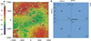 |
Fig. 1 DTM and applied tiling scheme. (a): shaded MLA DTM of Mercury’s north pole at a resolution of 250 m pixel−1. The map is displayed in gnomonic map projection centered at the north pole and color-coded by height. All units are in kilometers. (b): applied tiling scheme to derive temperatures for the DTM in (a). In total, 100 square tiles, each with a dimension of 200 × 200 km, make up the entire polar region of 2000 × 2000 km. |
2 Data
MLA recorded ≈26000000 range measurements with ≈10m radial and ≈100m horizontal accuracy (Bauer et al. 2015). The resulting dataset covers the entire northern, and small parts of the southern, Hermean hemisphere to 16°S (Neumann et al. 2016). A total of 3284 orbits are comprised in the dataset to which we applied (co)registration techniques (Gläser et al. 2013) to create a consistent polar DTM with a resolution of 250 m pixel−1 (Fig. 1a).
Due to the large dataset and limitations in processing power to derive the temperature for the entire DTM at once, we adopted a tiling scheme for our north polar MLA DTM (Fig. 1b). We divided the considered area of 2000 × 2000 km into four quadrants, Q1–Q4, with 25 square tiles each. The tiles have dimensions of 200 × 200km and contain subscripts identifying their relative position within the respective quadrant. For instance, tile  is a tile in the first quadrant, located in the fourth row and first column (compare Fig. 1).
3 Methodology
In this study we aim to model temperatures by balancing direct and indirect (scattered + re-radiated) radiation with conduction into the subsurface and re-radiation into space. The motion and rotation of Mercury as well as the exact position and size of the solar disk with respect to the Hermean surface is modeled using information from the DE421 ephemeris (Folkner et al. 2009) and by applying the respective SPICE routines (Acton 1996).
We chose the common approach of a one-dimensional representation of the heat equation to derive temperature estimates for the Hermean (sub)surface (Paige et al. 1992, Paige et al. 2010b; Gläser & Gläser 2019). Our model relies on several precalculated input parameters for which we briefly want to summarize a few key parameters and discuss, if appropriate, their updated versions in this study (see Gläser & Gläser 2019 and Gläser et al. 2014 for more details). Highlighted input parameters are the horizon maps (e.g., Mazarico et al. 2011; Gläser et al. 2014); view factors, which are referred to as visibility maps here (e.g., Vasavada et al. 1999); the solar limb darkening effect (e.g., Cox 2000); and the discretization of the depth profile (e.g., Gläser & Gläser 2019).
Horizon maps provide information about the highest elevation seen from each pixel in all directions, that is the horizon. For our purposes it is sufficient to describe the horizon by two parameters, the azimuth and elevation of each point along the horizon line. To derive illumination at each pixel, the respective horizon line needs to be contrasted to the apparent size and position of the solar disk along that line. In the previous lunar study by Gläser & Gläser (2019), a discretization of 0.5 ° for the horizon line was chosen based on the size of the apparent solar disk as seen from the lunar surface (≈0.5 °). Due to the even larger apparent solar disk size at Mercury (see Sect. 3.2), the discretization is sufficient for this study. Since the visible horizon at each pixel is static and only depends on the height of the observer, it has proven beneficial in regards to computational effort to precalculate the horizons. There is a manageable amount of information that needs to be stored and calculations can generally be made on the fully resolved DTM. The derivation of the horizon maps needed no updated version for our study.
3.1 Level-of-detail approach for visibility maps
Visibility maps provide information about the actual visible terrain and its geometry with respect to the observer. They are fundamental when re-radiated and scattered radiation shall be incorporated in the thermal analysis since they provide the relationship of each pixel with its visible surrounding. In contrast to horizon maps, however, the amount of information that needs to be precalculated and stored is large. In theory, the entire visible area between each pixel (observer) up to its respective horizon line needs to be stored, which, in terms of disk space, generally amounts to a large multiple of the original DTM size. Additionally, the expected visible area, and hence its disk usage, depends on the terrain morphology and cannot be predicted a priori. Therefore, this approach is inappropriate when applied and stored on the fully resolved DTM and certain simplifications should be made to keep memory usage to manageable levels and, at the same time, errors to a minimum. For instance, Gläser & Gläser (2019) limited the areal extent of the visibility map such that visible terrain was only derived for a fixed window size, making the maximum expected amount of disk usage a computable parameter. For their lunar study, they found that a window size of 60 × 60 km was suitable and could be allocated in their available memory, that is to say random access memory (RAM) or video RAM (VRAM) of the graphics processing unit (GPU).
We aim to add further functionality to the matter of visibility maps and memory limitations suitable for, but not limited to, our investigations on planet Mercury. The general idea is to reduce the amount of computational time and memory consumption by applying the concept of LOD (Clark 1976). The basic idea of this concept is that the LOD (resolution) decreases with the distance from the observer, leading to lower memory and processing demands. We adopted this approach by defining a set of square areas surrounding the observer, each with a fixed resolution, but decreasing with increasing square size. Consequently the user not only defines the desired window size for which they request visibility maps at full resolution, but also defines how many additional LODs shall be derived. We defined a threefold decrease in resolution from one LOD to the next, for example, if the first LOD has a resolution of 10 m pixel−1, then the second LOD has a resolution of 30 m pixel−1, the third LOD has a resolution of 90 m pixel−1, and so forth. The threefold decrease in resolution stems from the fact that in every grid with a center pixel, the grid size needs to be an odd number, for example 9 × 9 pixels (see Fig. 2a). Hence, the smallest possible reduction in resolution from one LOD to the next is three, which we adopted for this study. Let us assume the user chooses a window size of ±40 m around the observer position and a total of two LODs (Figs. 2a,b). Consequently, the first LOD would be at full resolution, for example 10 m pixel−1, for an area of 3 × 3 pixels (30 × 30 m) and the second LOD would then have a resolution of 30 m pixel−1 and also cover an area of 3 × 3 pixels (90 × 90 m) (Fig. 2b). For the previous approach (Gläser & Gläser 2019), from now on referred to as the NO Level-Of-Detail (NOLOD) approach (Fig. 2a), a visibility map covering an area of 90 × 90 m at full resolution requires memory to store up to 81 pixels; alternatively, the new approach, from now on referred to as the LOD approach (Fig. 2b), needs memory for a maximum of 17 pixels. This is a reduction in memory usage of 79%. In Fig. 2 we also show an arbitrary horizon line for which the maximum amount of visible pixels would be reduced to 47 pixels for the NOLOD approach and 13 pixels for the LOD approach, constituting a reduction in memory usage of 72%. We note that we actually only store values for pixels that are visible from the observer position, so those numbers would again be different and the stated percentages in memory reduction only represent an estimate. The actual reduction is dependent on the posed problem, for example the morphology of the terrain and the chosen size for the visibility map and number of LODs.
Due to the reduced resolution in the far field, fewer calculations are needed for the LOD approach which significantly speeds up the processing time. To investigate how well our LOD approach performs in terms of memory reduction and precision, we exemplarily present histograms of the residuals in comparison with two NOLOD approaches (see Figs. 3, 4). Similar to the finding in the lunar study of Gläser & Gläser (2019), we chose a 60 × 60 km window for our LOD approach with a total of two LODs (LOD2-60), that is a 20 × 20 km window at full resolution with 250 m pixel−1 for the first LOD and a 60 × 60 km window at 750 m pixel−1 for the second LOD (Fig. 3a). For the NOLOD approaches, we chose one window size that matches the extent and resolution of the first LOD in our LOD approach, that is a window of 20 × 20 km with 250 m pixel−1 (NOLOD-20, Fig. 3b). Here we want to asses the influence on the result solely stemming from the second LOD reaching out to 60 × 60 km at reduced resolution. The second NOLOD approach covers the same area as the LOD approach, that is to say a window of 60 × 60 km (NOLOD-60) at full resolution everywhere (Fig. 3c). Here we aim to asses how much information is lost due to the reduced resolution in the second LOD.
To compare the three different visibility maps, that is LOD2-60, NOLOD-20, and NOLOD-60, we chose to model temperatures over a one-year period using 12 h time steps for a 100 km2 area located near the Hermean north pole. The residuals between the resulting temperature maps were used to asses how well scattering from distant terrain was modeled. We note that if terrain scattering was not considered at all, the resulting temperature map would report colder temperatures than if scattering was considered, that is all residuals have the same algebraic sign. Consequently, models relying on higher resolved visibility maps report warmer temperature than models relying on lower resolution visibility maps.
The histogram of the residuals between the NOLOD-20 and the LOD2-60 approach (see Fig. 4a) reveal that the LOD2-60 approach either reports the same temperatures as the NOLOD-20 approach, or it exclusively reports warmer surfaces. In fact ≈50% of the pixels are warmer and a total of ≈30% are warmer than 1 K. This result was expected since a larger area in the LOD2-60 approach also means more possible scatterers, which in turn contribute additional heat and lead to warmer surfaces. We find a maximum temperature difference of 6.3 K at the surface with a mean of 1.01 K.
The second histogram (see Fig. 4b) shows the residuals between the NOLOD-60 and LOD2-60 approaches. It is noticeable that all residuals are positive, revealing that the LOD2-60 approach either produces the same temperatures or reports colder temperatures than the NOLOD-60 approach. This was also expected since the LOD2-60 approach is heavily smoothed in the far field in comparison with the NOLOD-60 approach and hence it underestimates the influx stemming from scatterers. Comparing the respective memory usage, we in fact see that the LOD2-60 approach only used 465 Mb of memory, while the NOLOD-60 approach needed 1 Gb. This represents a reduction in memory usage of ≈55%. Further we note that despite the significant reduction of information in the LOD2-60 approach, we still find that ≈75% of the residuals are smaller than 0.1 K with a mean of 0.09 K and there is a maximum temperature difference of 0.53 K.
So far, we have investigated scatterers which can be up to ≈42.4km away from the observer (corner of the 60 × 60 km windows). To verify if there are additional scatterers that significantly contribute to the derived temperatures, we performed an additional analysis using an approach with two LODs and a total window size of 150 × 150 km, that is a window of 50 × 50 km at full resolution of 250 m pixel−1 for the first LOD and a window of 150 × 150km at 750 m pixel−1 for the second LOD (LOD2-150). We found that the resulting temperature map is virtually identical to the NOLOD-60 approach, revealing that no scatterers are found beyond the 60 × 60 km windows that significantly contribute to the temperature map (see histogram of residuals in Fig. 4c). The maximum temperature difference is found to be just 0.016 K with a mean of the residuals of 0.0004 K. Since the LOD2-150 approach used six times the memory needed for the NOLOD-60 approach and since it delivers identical results, there is no need to extend the window sizes beyond 60 km.
In summary, we note that we were able to empirically derive a minimum size for the first LOD (20 × 20 km) and total number for the required LODs (two) for which the reduced resolution in the far field has no significant impact on the results, that is to say a maximum temperature difference of ≈0.5 K. For our study, we chose the LOD approach using the presented LOD2-60 windows which halves the required memory usage in comparison to the previous NOLOD approach.
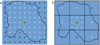 |
Fig. 2 Square visibility maps (blue area) for a given observer (green outlined pixel). All pixels (white + signs) that are within the horizon lines (black line) can potentially contribute additional heat to the observer position if a direct line of sight exists. All pixels (black + signs) that are outside the horizon line, or coincide with the observer, do not contribute to the temperature at the observer position. (a): NOLOD visibility map using the full resolution of the input DTM. (b): LOD visibility map applying two LODs with full resolution for the first LOD at ±1 pixel around the observer and a third of the resolution for the second LOD. |
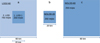 |
Fig. 3 Various visibility maps that we compared to each other. (a): LOD2-60 visibility map with 250 m pixel−1 at the first LOD spanning 20 × 20 km and a resolution of 750 m pixel−1 at the second LOD covering an area of 60 × 60 km. (b): NOLOD-20 visibility map resembling the first LOD of the map shown in (a). (c): NOLOD-60 visibility map covering the same area as the map shown in (a) with a resolution of 250 m pixel−1. |
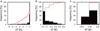 |
Fig. 4 Histograms (black) and cumulative histogram (red) of the residuals from temperature maps derived using different visibility maps. (a): residuals of the NOLOD-20 to the LOD2-60 approach. (b): residuals of the NOLOD-60 to the LOD2-60 approach. (c): residuals of the NOLOD-60 to the LOD2-150 approach. |
3.2 Improved resolution for solar-limb darkening effect
In their previous study, Gläser & Gläser (2019) modeled the solar limb darkening effect (Cox 2000) by dividing the solar disk into five consecutive rings with fixed intensity values per ring, but radially outward decreasing intensity values (compare Fig. 7 in their study). Given the immediate proximity of planet Mercury to the Sun, we want to present an additional analysis of the solar limb darkening effect and investigate whether the previously chosen discretization for their lunar study proves sufficient for this study.
First we want to point out that the apparent solar disk radius is more than two to three times larger for an observer on Mercury than on the Moon, for example ≈ 1.14–1.74° in comparison to ≈ 0.52–0.54 °, respectively. The vast size variation of the solar disk stems from Mercury’s highly eccentric orbit and consequently it has great implications on the amount of received solar radiation on its surface. This motivated us to carry out a more profound analysis of the impact of various degrees of discretization of the solar disk on the derived temperatures.
We chose the exact same approach as outlined in Gläser & Gläser (2019) and only varied the degree of discretization. As a benchmark, we chose to divide the solar disk into 200 rings and derived a temperature map of tile  (see Sect. 2) considering three rotations (two revolutions), that is to say ≈ 176 days. Subsequently, we derived temperature maps of
  for the same time period with the solar limb darkening effect modeled by one, five, eight, 12, 20, 30, and 80 rings, respectively. The residuals of those temperature maps to our benchmark show strong convergence and are already flattening out, which leads us to consider our set benchmark to be appropriate (Fig. 5). Furthermore, the solar limb darkening effect – in general – and its degree of discretization show a large impact on temperature. For instance, if we do not model the solar limb darkening effect at all, that is if the Sun is modeled to have a constant intensity over its entire disk (compare one ring in Fig. 5), we would find temperature residuals ranging from −8.67 to 8.85 K with respect to our benchmark. In addition, the temperature map with a solar disk discretization of five rings (chosen in the study of Gläser & Gläser 2019) would have a range of temperature residuals from −2.89 to 2.49 K with respect to our benchmark. Similar to our findings for the visibility map in Sect. 3.1, we accept a trade-off between model complexity (processing time) and errors of ≈0.5K. The first degree of discretization that satisfies our threshold is found at 30 rings, which we adopted for our study.
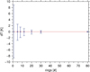 |
Fig. 5 Temperature residuals for various degrees of discretization of the solar limb darkening effect with respect to a 200-ring benchmark model. The previous implementation (lunar case) used a discretization of five rings, which shows large residuals for temperatures at Mercury, i.e., >2 K. At a discretization of 30 rings, residuals are below ≈0.5 K, which was adopted for this study. |
3.3 Updated depth profile
In order to derive temperatures for locations in the subsurface, one needs to choose a set of nodes for which temperatures will be calculated, referred to as the depth profile. Due to the nonlinear behavior of the posed problem (see Gläser & Gläser 2019), the discretization of said profile has large implications on the convergence and accuracy of the result. In general, a finer discretization is needed where large and sudden changes can occur. For our problem, the largest and most abrupt changes occur close to the surface, especially at sunset and sunrise. In their previous approach, Gläser & Gläser (2019) manually chose a profile that suited their lunar study. Here, we present a more generic approach to derive depth profiles which we adopted for this study. The depth profile is defined by two parameters which can be chosen by the user, that is the depth to which the profile shall reach into the subsurface and the number of nodes that shall be distributed along that profile. Several trade-offs and characteristics need to be considered when choosing a depth profile. On the one hand, it can be noted that the more nodes that are chosen, the better the nonlinear behavior can be modeled, especially near the surface. On the other hand, the computational effort scales linearly with the number of nodes and only nodes that contribute to the accuracy of the temperature profile should be chosen. Furthermore, temperatures at the deeper parts of the profile can generally be described by much larger node distances since only small changes occur. As a result, we chose to distribute the nodes in an exponential manner along the profile with short distances between the nodes in the upper regolith close to the surface and with increasing distances at greater depths. First the distance of the surface to the last node of the profile was derived in terms of nodes
 (1)
(1)
The damping of the exponential function is denoted by ζ and was chosen to be five for this study. The damping number was found empirically. The volumes surrounding the nodes in its center then occupy a fraction (r) of the entire profile according to
 (2)
(2)
The metric values for the volume sizes (v) and node positions (p) follow by incorporating the chosen maximum depth (maxd), which – similar to the lunar study of Gläser & Gläser (2019) – we chose to be 2 m for this study:
 (3)
(3)
 (4)
(4)
In Fig. 6a we depict the increase in volume size with increasing depth and in Fig. 6b we show a comparison between the upper part of their previous depth profile (Gläser & Gläser 2019) to the one outlined in this study. It can be seen that the new profile places more nodes in the upper regolith and allows for larger volumes, that is larger node separation, in the deeper layers of regolith where temperature changes are relatively slow and small. Similar to the study by Gläser & Gläser (2019; see their Fig. 13), we show comparisons of their irregularly spaced depth profile of 29 nodes, a depth profile with 80 regularly spaced nodes, and two depth profiles derived using the presented exponential approach, one with 40 and the other with 29 nodes (see Fig. 7). We note that, by visual comparison of the profiles in the upper 5 cm of regolith (Fig. 7b), the irregular and exponential profiles follow the same trend. Similar to the previous finding of Gläser & Gläser (2019), a regular node spacing, even with twice as many nodes, cannot resolve the actual temperature distribution close to the surface and it consequently propagates and provides inaccurate temperature estimates for the deeper subsurface. We also note that both exponential approaches show a finer resolution in the upper regolith than the previously chosen irregular spacing. In fact, choosing the exponential 40-nodes approach as our benchmark and applying the composite Simpson’s rule to determine the area beneath the temperature profile, we find relative errors of 0.2 and 0.6% when contrasted with the areas found for the exponential 29-nodes and irregular 29-nodes approach, respectively. Although the relative errors are small, the errors for the irregular 29-nodes approach is three times larger than for the exponential 29-nodes approach. As a trade-off between processing time, memory usage, and accuracy, we chose the exponential 29-nodes approach for this study.
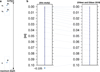 |
Fig. 6 (a): sketch of a depth profile derived by the exponential approach. Node distances and volume sizes increase in an exponential manner with greater depths. (b): comparison of the upper 10 cm (≈16 nodes) of the exponential 29-nodes approach adopted for this study and the irregular 29-nodes approach in the previous study of Gläser & Gläser (2019). We note the higher node density close to the surface in the new approach leading to finer resolution of the nonlinear behavior of the temperature distribution. |
4 Results
Starting from a uniform temperature distribution at each node, we iterated several times over a period of 175.94 days, from January 1, 2000 at midnight to June 24, 2000 at 11 pm. The chosen time period stems from the 3 : 2 spin-orbit resonance of Mercury (three rotations in two revolutions) with an orbital period of 87.9692 days (Colombo 1965; Archinal et al. 2018). At the beginning and end of that period, Mercury receives similar illumination conditions and hence an iteration using the temperature map at the end of the period as an input for the next iteration is appropriate. After eight iterations with a time step of 12 h, the near-surface temperatures have converged and we have found a solution (see Fig. 8). For each tile (see Sect. 2 and Fig. 1b), we used the temperature estimates from the last iteration (8th) and ran another iteration to compile average and maximum temperature maps as well as surface ice and depth-to-ice maps (see Fig. 9). In fact, this is the first time that model temperatures on the complete polar MLA DTM are reported; this is especially of importance for temperatures at latitudes above ≈85 °N. In a previous study conducted during the ongoing MESSENGER mission, MLA tracks were still too sparse or they did not exist at these latitudes (Paige et al. 2013). Other studies have concentrated on single craters or nonpolar regions (Hamill et al. 2020; Bauch et al. 2021).
Due to the 3 : 2 spin-orbit resonance of Mercury, so-called hot (at 0 °E and 180 °E) and warm (at 90 °E and 270 °E) longitudes emerge (Siegler et al. 2013). The warm and hot longitudes clearly manifest themselves in the displayed temperature maps, especially in the depth-to-ice map (Fig. 9d). Here, isothermals and equal depths show an elliptical distribution with the semimajor and semiminor axis coinciding with said longitudes. It is noticeable though that one hot longitude, that is at 180 °E, provides a larger area at which temperatures are such that water ice is stable in the upper 2 m of regolith. This can be attributed to the relatively higher polar topography on that hemisphere which in turns leads to more shadowing and consequently colder temperatures (see also Fig. 1). For most PSRs, especially for those within the “big five” (Prokofiev, Kandinsky, Tolkien, Tryggvadόttir, and Chesterton crater), we find temperatures that are below 112 K and allow for surface ice (see Figs. 9c,d). These craters were found to contain radar bright material at their large floors (Deutsch et al. 2016; Rivera-Valentin et al. 2022). They are all located north of 84 ° and make a significant contribution to the roughly 90% of the total radar bright material which is found there.
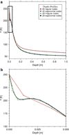 |
Fig. 7 Temperature profiles in the subsurface using different node-spacing approaches and a different number of nodes. (a): temperature distribution in the upper 1 m of regolith. The regular node spacing with 80 nodes (red) cannot resolve the upper temperature distribution and it propagates inaccurate temperature estimates to the subsurface, leading to a profile that is vastly different than the other three approaches. The two exponential node spacing approaches, 40 nodes (blue) and 29 nodes (black), and the irregular 29-nodes spacing approach (green) follow the same trend and provide similar temperatures. (b): same profiles as in (a), but for the upper 5 cm of regolith. The regularly spaced profile (red) is too poorly resolved close to the surface to model the temperature distribution. The other three approaches show a similar trend with the two exponential approaches showing smoother and higher resolved temperature profiles than the previously chosen irregular node spacing. |
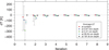 |
Fig. 8 Convergence of temperatures tracked at four nodes at 0.67 mm, 3.47 cm, 29.54 cm, and 181.8 cm. The black bars at each node represent the range of temperature differences found at the respective iteration with respect to the previous iteration. |
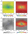 |
Fig. 9 Temperature maps of the north polar region. The maps are displayed in gnomonic map projection centered at the north pole and color-coded by temperature (a,b), height (c), and depths (d). Axis units are in kilometers. (a): average temperature map. (b): maximum temperature map. (c): location of possible surface ice (blue). (d): depth-to-ice map for the upper 2 m of regolith derived from the maximum temperature where temperatures are below 112 K. |
5 Conclusions
Our existing (lunar) thermal model needed to be updated in order to derive temperature estimates for Mercury. Several improvements were successfully implemented and validated. With the new capabilities added to the thermal model we were able to derive temperatures for the Hermean north pole.
We successfully applied a LOD approach to handle terrain scattering and thermal re-radiation on large datasets such as the polar MLA DTM. We have shown that memory usage could be reduced by ≈50%, while keeping residuals below ≈0.5 K with respect to our benchmark.
A refined analysis of the solar limb darkening effect has revealed that our previous discretization of five rings to derive temperatures for the Moon proved insufficient for the thermal model at Mercury which resides much closer to the Sun. We find that modeling the solar disk by 30 rings could allow us to keep residuals below ≈0.5 K with respect to our benchmark.
We applied a new approach to derive node distances for subsurface profiles, for example the depth profile for which we derived temperatures. It was found that our depth profile using the new approach leads to superior results in comparison with our previous depth profile, especially in the shallow subsurface.
For the first time, temperatures were derived for the complete polar MLA DTM. Especially areas north of ≈85 °N were not modeled in previous studies.
We find maximum surface temperatures for the “big five” (Prokofiev, Kandinsky, Tolkien, Tryggvadόttir, and Chesterton crater), which are cold enough for water ice to be stable for geological timescales. This finding strongly supports radar observations of those craters showing radar-bright deposits.
In future studies, we aim to apply our refined thermal model to in-depth investigations of temperatures at the Hermean poles and their correlation with radar-bright deposits.
Acknowledgements
P.G. was funded by a Grant of the German Research Foundation (GL 865/3-1). We also gratefully acknowledge the support of NVIDIA Corporation with the donation of a Quadro M5000 and Quadro P6000 GPU used for this research.
References
- Acton, C. H. 1996, Planet. Space Sci., 44, 65 [Google Scholar]
- Araki, H., Tazawa, S., Noda, H., et al. 2009, Science, 323, 897 [NASA ADS] [CrossRef] [Google Scholar]
- Archinal, B. A., Acton, C. H., A’Hearn, M.F., et al. 2018, Celest. Mech. Dyn. Astron., 130, 22 [NASA ADS] [CrossRef] [Google Scholar]
- Arnold, J. R. 1979, J. Geophys. Res., 84, 5659 [NASA ADS] [CrossRef] [Google Scholar]
- Bauch, K. E., Hiesinger, H., Helbert, J., Robinson, M. S., & Scholten, F. 2014, Planet. Space Sci., 101, 27 [NASA ADS] [CrossRef] [Google Scholar]
- Bauch, K. E., Hiesinger, H., Greenhagen, B. T., & Helbert, J. 2021, Icarus, 354, 114083 [NASA ADS] [CrossRef] [Google Scholar]
- Bauer, R. S., Barker, M. K., Mazarico, E., & Neumann, G. A. 2015, AGU Fall Meeting Abstracts, 2015, P41C [Google Scholar]
- Buhl, D., Welch, W. J., & Rea, D. G. 1968, J. Geophys. Res. 73, 24 [Google Scholar]
- Clark, J. H. 1976, Commun. ACM, 19, 547 [CrossRef] [Google Scholar]
- Colombo, G. 1965, Nature, 208, 575 [NASA ADS] [CrossRef] [Google Scholar]
- Cox, A. N. 2000, Allen’s Astrophysical Quantities (Berlin: Springer) [Google Scholar]
- Deutsch, A. N., Chabot, N. L., Mazarico, E., et al. 2016, Icarus, 280, 158 [NASA ADS] [CrossRef] [Google Scholar]
- Folkner, W. M., Williams, J. G., & Boggs, D. H. 2009, Interplanet. Netw. Prog. Rep., 42–178, 1 [Google Scholar]
- Gläser, P., & Gläser, D. 2019, A&A, 627, A129 [NASA ADS] [CrossRef] [EDP Sciences] [Google Scholar]
- Gläser, P., Haase, I., Oberst, J., & Neumann, G. A. 2013, Planet. Space Sci., 89, 111 [CrossRef] [Google Scholar]
- Gläser, P., Scholten, F., De Rosa, D., et al. 2014, Icarus, 243, 78 [CrossRef] [Google Scholar]
- Gläser, P., Sanin, A., Williams, J.-P., Mitrofanov, I., & Oberst, J. 2021, J. Geophys. Res. Planets, 126, e06598 [CrossRef] [Google Scholar]
- Hamill, C. D., Chabot, N. L., Mazarico, E., et al. 2020, Planet. Sci. J., 1, 57 [NASA ADS] [CrossRef] [Google Scholar]
- Harmon, J. K., & Slade, M. A. 1992, Science, 258, 640 [NASA ADS] [CrossRef] [Google Scholar]
- Harmon, J. K., Slade, M. A., & Rice, M. S. 2011, Icarus, 211, 37 [NASA ADS] [CrossRef] [Google Scholar]
- Hayne, P. O., Bandfield, J. L., Siegler, M. A., et al. 2017, J. Geophys. Res. Planets, 122, 2371 [Google Scholar]
- Ingersoll, A. P., Svitek, T., & Murray, B. C. 1992, Icarus, 100, 40 [NASA ADS] [CrossRef] [Google Scholar]
- Kato, M., Sasaki, S., Tanaka, K., Iijima, Y., & Takizawa, Y. 2008, Adv. Space Res., 42, 294 [NASA ADS] [CrossRef] [Google Scholar]
- Mazarico, E., Neumann, G. A., Smith, D. E., Zuber, M. T., & Torrence, M. H. 2011, Icarus, 211, 1066 [NASA ADS] [CrossRef] [Google Scholar]
- Neumann, G. A., Perry, M. E., Mazarico, E., et al. 2016, in 47th Annual Lunar and Planetary Science Conference, Lunar and Planetary Science Conference, 2087 [Google Scholar]
- Paige, D. A., Wood, S. E., & Vasavada, A. R. 1992, Science, 258, 643 [NASA ADS] [CrossRef] [Google Scholar]
- Paige, D. A., Foote, M. C., Greenhagen, B. T., et al. 2010a, Space Sci. Rev., 150, 125 [Google Scholar]
- Paige, D. A., Siegler, M. A., Zhang, J. A., et al. 2010b, Science, 330, 479 [NASA ADS] [CrossRef] [Google Scholar]
- Paige, D. A., Siegler, M. A., Harmon, J. K., et al. 2013, Science, 339, 300 [NASA ADS] [CrossRef] [Google Scholar]
- Rivera-Valentín, E. G., Meyer, H. M., Taylor, P. A., et al. 2022, Planet. Sci. J., 3, 62 [CrossRef] [Google Scholar]
- Salvail, J. R., & Fanale, F. P. 1994, Icarus, 111, 441 [NASA ADS] [CrossRef] [Google Scholar]
- Siegler, M. A., Bills, B. G., & Paige, D. A. 2013, J. Geophys. Rese. Planets, 118, 930 [NASA ADS] [CrossRef] [Google Scholar]
- Slade, M. A., Butler, B. J., & Muhleman, D. O. 1992, Science, 258, 635 [NASA ADS] [CrossRef] [Google Scholar]
- Solomon, S. C., McNutt, R. L., Gold, R. E., & Domingue, D. L. 2007, Space Sci. Rev., 131, 3 [NASA ADS] [CrossRef] [Google Scholar]
- Thomas, G. E. 1974, Science, 183, 1197 [NASA ADS] [CrossRef] [Google Scholar]
- Vasavada, A. R., Paige, D. A., & Wood, S. E. 1999, Icarus, 141, 179 [NASA ADS] [CrossRef] [Google Scholar]
- Vasavada, A. R., Bandfield, J. L., Greenhagen, B. T., et al. 2012, J. Geophys. Res. Planets, 117, E00H18 [Google Scholar]
- Vondrak, R., Keller, J., Chin, G., & Garvin, J. 2010, Space Sci. Revs., 150, 7 [NASA ADS] [CrossRef] [Google Scholar]
- Watson, K., Murray, B., & Brown, H. 1961, J. Geophys. Res., 66, 1598 [NASA ADS] [CrossRef] [Google Scholar]
- Zuber, M. T., Smith, D. E., Phillips, R. J., et al. 2012, Science, 336, 217 [NASA ADS] [CrossRef] [Google Scholar]
All Figures
|
Fig. 1 DTM and applied tiling scheme. (a): shaded MLA DTM of Mercury’s north pole at a resolution of 250 m pixel−1. The map is displayed in gnomonic map projection centered at the north pole and color-coded by height. All units are in kilometers. (b): applied tiling scheme to derive temperatures for the DTM in (a). In total, 100 square tiles, each with a dimension of 200 × 200 km, make up the entire polar region of 2000 × 2000 km. |
| In the text | |
|
Fig. 2 Square visibility maps (blue area) for a given observer (green outlined pixel). All pixels (white + signs) that are within the horizon lines (black line) can potentially contribute additional heat to the observer position if a direct line of sight exists. All pixels (black + signs) that are outside the horizon line, or coincide with the observer, do not contribute to the temperature at the observer position. (a): NOLOD visibility map using the full resolution of the input DTM. (b): LOD visibility map applying two LODs with full resolution for the first LOD at ±1 pixel around the observer and a third of the resolution for the second LOD. |
| In the text | |
|
Fig. 3 Various visibility maps that we compared to each other. (a): LOD2-60 visibility map with 250 m pixel−1 at the first LOD spanning 20 × 20 km and a resolution of 750 m pixel−1 at the second LOD covering an area of 60 × 60 km. (b): NOLOD-20 visibility map resembling the first LOD of the map shown in (a). (c): NOLOD-60 visibility map covering the same area as the map shown in (a) with a resolution of 250 m pixel−1. |
| In the text | |
|
Fig. 4 Histograms (black) and cumulative histogram (red) of the residuals from temperature maps derived using different visibility maps. (a): residuals of the NOLOD-20 to the LOD2-60 approach. (b): residuals of the NOLOD-60 to the LOD2-60 approach. (c): residuals of the NOLOD-60 to the LOD2-150 approach. |
| In the text | |
|
Fig. 5 Temperature residuals for various degrees of discretization of the solar limb darkening effect with respect to a 200-ring benchmark model. The previous implementation (lunar case) used a discretization of five rings, which shows large residuals for temperatures at Mercury, i.e., >2 K. At a discretization of 30 rings, residuals are below ≈0.5 K, which was adopted for this study. |
| In the text | |
|
Fig. 6 (a): sketch of a depth profile derived by the exponential approach. Node distances and volume sizes increase in an exponential manner with greater depths. (b): comparison of the upper 10 cm (≈16 nodes) of the exponential 29-nodes approach adopted for this study and the irregular 29-nodes approach in the previous study of Gläser & Gläser (2019). We note the higher node density close to the surface in the new approach leading to finer resolution of the nonlinear behavior of the temperature distribution. |
| In the text | |
|
Fig. 7 Temperature profiles in the subsurface using different node-spacing approaches and a different number of nodes. (a): temperature distribution in the upper 1 m of regolith. The regular node spacing with 80 nodes (red) cannot resolve the upper temperature distribution and it propagates inaccurate temperature estimates to the subsurface, leading to a profile that is vastly different than the other three approaches. The two exponential node spacing approaches, 40 nodes (blue) and 29 nodes (black), and the irregular 29-nodes spacing approach (green) follow the same trend and provide similar temperatures. (b): same profiles as in (a), but for the upper 5 cm of regolith. The regularly spaced profile (red) is too poorly resolved close to the surface to model the temperature distribution. The other three approaches show a similar trend with the two exponential approaches showing smoother and higher resolved temperature profiles than the previously chosen irregular node spacing. |
| In the text | |
|
Fig. 8 Convergence of temperatures tracked at four nodes at 0.67 mm, 3.47 cm, 29.54 cm, and 181.8 cm. The black bars at each node represent the range of temperature differences found at the respective iteration with respect to the previous iteration. |
| In the text | |
|
Fig. 9 Temperature maps of the north polar region. The maps are displayed in gnomonic map projection centered at the north pole and color-coded by temperature (a,b), height (c), and depths (d). Axis units are in kilometers. (a): average temperature map. (b): maximum temperature map. (c): location of possible surface ice (blue). (d): depth-to-ice map for the upper 2 m of regolith derived from the maximum temperature where temperatures are below 112 K. |
| In the text | |
Current usage metrics show cumulative count of Article Views (full-text article views including HTML views, PDF and ePub downloads, according to the available data) and Abstracts Views on Vision4Press platform.
Data correspond to usage on the plateform after 2015. The current usage metrics is available 48-96 hours after online publication and is updated daily on week days.
Initial download of the metrics may take a while.