| Issue |
A&A
Volume 674, June 2023
|
|
|---|---|---|
| Article Number | A69 | |
| Number of page(s) | 31 | |
| Section | Planets and planetary systems | |
| DOI | https://doi.org/10.1051/0004-6361/202245343 | |
| Published online | 06 June 2023 | |
An advanced thermal roughness model for airless planetary bodies
Implications for global variations of lunar hydration and mineralogical mapping of Mercury with the MERTIS spectrometer★
1
Image Analysis Group, TU Dortmund University,
Otto-Hahn-Str. 4,
44227
Dortmund, Germany
e-mail: This email address is being protected from spambots. You need JavaScript enabled to view it.
2
Institute for Planetology,
Wilhelm-Klemm-Str. 10,
48149
Münster, Germany
3
Institute for Planetary Research, DLR,
Rutherfordstr. 2,
12489
Berlin, Germany
Received:
31
October
2022
Accepted:
22
March
2023
Abstract
We present a combined reflectance and thermal radiance model for airless planetary bodies. The Hapke model provides the reflected component. The developed thermal model is the first to consistently use rough fractal surfaces, self-scattering, self-heating, and disk-resolved bolometric albedo for entire planets. We validated the model with disk-resolved lunar measurements acquired by the Chinese weather satellite Gaofen-4 at around 3.5–4.1 μm and measurements of the Diviner lunar radiometer at 8.25 μm and 25–41 μm, finding nearly exact agreement. Further, we reprocessed the thermal correction of the global lunar reflectance maps obtained by the Moon Mineralogy Mapper M3 and employed the new model to correct excess thermal radiance. The results confirm the diurnal, latitudinal, and compositional variations of lunar hydration reported in previous and recent studies with other instruments. Further, we compared the model to lunar measurements obtained by the Mercury Radiometer and Thermal Infrared Spectrometer (MERTIS) on board BepiColombo during a flyby maneuver on April 9, 2020: the measured and the modeled radiance variations across the disk match. Finally, we adapted the thermal model to Mercury for emissivity calibration of upcoming Mercury flyby measurements and in-orbit operation. Although a physical parameter must be invariant under various observation scenarios, the best lunar surface roughness fits vary between different datasets. We critically discuss possible reasons and conclude that anisotropic emissivity modeling has room for improvement and requires attention in future studies.
Key words: Moon / infrared: planetary systems / radiation mechanisms: thermal / methods: data analysis / methods: numerical / planets and satellites: surfaces
Datasets and modeling results are available under https://doi.org/10.5281/zenodo.7776031
© The Authors 2023
 Open Access article, published by EDP Sciences, under the terms of the Creative Commons Attribution License (https://creativecommons.org/licenses/by/4.0), which permits unrestricted use, distribution, and reproduction in any medium, provided the original work is properly cited.
This article is published in open access under the Subscribe to Open model. This email address is being protected from spambots. You need JavaScript enabled to view it. to support open access publication.
1 Indroduction
Thermophysical models (TPMs) are versatile tools for analyzing the thermal emission of airless bodies such as planets, moons, and asteroids. Developed initially to understand the thermal phase curve of the Moon (e.g., Smith 1967; Buhl et al. 1968; Sexl et al. 1971), thermal models are now in use for bodies throughout the Solar System to perform calibration tasks and to address a diverse set of research questions. Here, we present an advanced thermal model that consistently employs rough fractal surfaces, self-heating, self-scattering, and directional bolometric albedos, rendering it the most detailed implementation to date. We validated the model and applied it to two current research topics: the detection of lunar hydration and the mineralogical mapping of Mercury. Our study uses four datasets of the Moon. In the summer of 2018, the Chinese weather satellite Gaofen-4 (GF-4) acquired disk-resolved images of the Moon for five different illumination geometries and at six bands in the visible to near-infrared (VIS-NIR) and mid-infrared (MIR; Wu et al. 2021). The MIR measurements around 3.77 μm are a valuable testbed for the new thermal model because they resolve the entire Moon for a broad range of incidence and emission angles. The Diviner lunar radiometer on board the Lunar Reconnaissance Orbiter (LRO) mapped the lunar surface from 0.4 to 400 μm (Paige et al. 2010a). Diviner performed several off-nadir measurements that cover complex observation geometries that we use for model validation in the thermal infrared (TIR) around 8.25 μm and from 25 to 41 μm, similar to Bandfield et al. (2015). The GF-4 measurements around 3.77 μm enable an independent assessment of thermal excess removal methods for the Moon Mineralogy Mapper (M3) in a comparable wavelength region (Wöhler et al. 2017; Grumpe et al. 2019). We reprocessed the global M3 dataset with the new thermal model and assessed the plausibility of lunar OH/H2O detection in recent studies (e.g., Wöhler et al. 2017; Grumpe et al. 2019). Therfore, we investigated the diurnal, latitudinal, and compositional variations of lunar hydration. On April 9, 2020, the BepiColombo probe performed a flyby maneuver. The Mercury Radiometer and Thermal Infrared Spectrometer (MERTIS) on board the spacecraft acquired the first spaceborne hyperspectral data of the Moon at 7–14 μm through the calibration baffle. Diviner emission phase function (EPF) measurements ensure proper thermal model validation in this wavelength range. The MERTIS lunar data allow for the radiance calibration and the thermal model to be cross-checked before BepiColombo’s Mercury flyby and in-orbit measurements after insertion into orbit in 2025.
2 Previous work and motivation
In this section, we (1) review the diverse landscape of thermo-physical modeling and discuss thermal correction for (2) lunar OH/H2O detection and (3) emissivity retrieval for Mercury. Both applications require an independent test of a thermophysical model we carried out with GF-4 and Diviner data.
2.1 Thermophysical models for airless planetary bodies
Thermophysical models of airless planetary bodies are used in astronomy and planetary geoscience. Nearly every science case and target body has its own thermal model. This diverse landscape is motivated by two broad application scenarios: TPMs help astronomers to characterize asteroids from telescopic observations. Planetary scientists employ TPMs to analyze planetary regolith and volatile stability from remote sensing data. The astronomical and geoscience perspectives overlap but are rarely reviewed together.
For a review of (asteroid) thermal modeling, readers can refer to Delbo et al. (2015), who differentiate between equilibrium models and TPMs that include roughness, heat conduction, and sometimes scattering and self-heating. The first thermal asteroid models are often referred to as the standard thermal model (STM) of Lebofsky et al. (1978) and Lebofsky et al. (1986) that assumed a fixed shape, simple thermal equilibrium, and a beaming parameter that accounts for anisotropy due to roughness. The near earth asteroid thermal model (NEATM; Harris 1998) and its modifications (Myhrvold 2018) form the de facto standard for asteroid thermal modeling today if the data prohibit the use of a full TPM (Delbo et al. 2015). Thermophysical models are more complex and are the method of choice if adequate data are available. Thermophysical models date back to the first lunar studies. Pettit & Nicholson (1930) found that a smooth surface in thermal equilibrium does not explain the thermal phase curve of the Moon. Smith (1967), Buhl et al. (1968), and Sexl et al. (1971) modeled the rugged lunar surface with spherical craters and suggested that shadows and an altered temperature distribution explain the shape of the thermal phase curve. Spencer et al. (1989) and Spencer (1990) adopted the lunar models for general airless bodies, thereby establishing the basis for most current asteroid TPMs (Delbo et al. 2015). All these models (Spencer 1990; Lagerros 1996; Emery et al. 1998; Rozitis & Green 2011, 2012, 2013; MacLennan & Emery 2018; Rozitis et al. 2020) combined an equilibrium term, a thermal roughness model, and a heat conduction model. Nonresolved surface roughness controls the angular deviations of the emitted flux, which are responsible for the thermal beaming effect of asteroids or the non-Lambertian phase curve of the Moon. Roughness is commonly modeled by spherical segment craters (Smith 1967; Spencer 1990; Lagerros 1996; Emery et al. 1998; Rozitis & Green 2011, 2012, 2013; MacLennan & Emery 2018), random Gaussian surfaces (Davidsson et al. 2015; Grumpe et al. 2019; Rubanenko et al. 2020), and by realistic fractal rough surface models (Davidsson et al. 2015; Rozitis et al. 2020). Heat conduction becomes important if the rotational period of the body is comparatively fast or if the goal is to infer the thermal inertia from nightside measurements. Heat conduction can generally be neglected on the dayside if rotation is slow. Myhrvold (2018) reviews thermophysical asteroid modeling in the presence of reflected sunlight and points out how to correctly account for energy conservation in spectral regions, where thermal emission and solar reflection superimpose.
Since the early 2000s, several infrared detectors have visited airless bodies to map the thermal inertia, acquire emissivity spectra for mineralogical interpretation, and to determine the surface roughness: OTES on OSIRIS-REx for Bennu (Christensen et al. 2018), VIR on DAWN for Vesta (De Sanctis et al. 2012), TIR on Hayabusa2 for Ryugu (Okada et al. 2018), VIRTIS on Rosetta for 67P/Churyumov-Gerasimenko (Coradini et al. 2007), Diviner on LRO for the Moon (Paige et al. 2010a), the Moon Mineralogy Mapper (M3) for the Moon on Chandrayaan 1 (Pieters et al. 2009a), and MERTIS on BepiColombo for Mercury (Hiesinger & Helbert 2010). The geophysical community is primarily interested in the thermophysical characteristics of the upper regolith and developed thermal heat conduction models, mostly in parallel to the asteroid thermophysical models. Keihm & Langseth (1973) first inferred the thermal conductivity of the lunar regolith near the Apollo 17 landing site. Vasavada et al. (1999) and Paige et al. (2010b) modeled lunar temperature stability to analyze the stability of polar volatiles with either a heat conduction model or an equilibrium model. Hayne et al. (2017) presented a detailed subsurface heat conduction model and derived the Moon’s global thermal conductivity and thermal inertia maps from Diviner lunar radiometer measurements – again without roughness even though roughness has been thoroughly modeled for asteroids, Bandfield et al. (2015) were the first to derive roughness values from Diviner nadir and offnadir measurements. The brightness temperatures inferred from Diviner channel four (8.25 μm) and channel seven (25-41 μm) are similar for small incidence angles but deviate for increasing incidence angles. Brightness temperature differences can be as high as 70 K in the early morning or late evening. Diviner further acquired off-nadir measurements (EPF functions) to cover a broad range of emission angles up to approximately 80°. Bandfield et al. (2015) found that a root mean squared (RMS) slope of 20° of a Gaussian slope distribution model best matches the nadir observations, and an RMS slope of 20–35° best matches a small set of multiangle measurements. Bandfield et al. (2015) further employed a small-scale heat conduction model showing that those surface elements are greater than ~0.5–5 mm remain thermally isolated. Rubanenko et al. (2020) repeated a roughness study with telescopic measurements of Sinton (1961) and Diviner data and found a bidirectional RMS slope of 30.2° ± 5.9° for maria and 36.8° ± 4.4° for highlands. Heat conduction models are used for other planetary bodies such as Ceres (Rognini et al. 2020) and Vesta (Capria et al. 2014). Marshall et al. (2018) mapped the thermal inertia of 67P/Churyumov-Gerasimenko. Bauch et al. (2014, 2021) adapted a heat-conduction model for the planet Mercury that is planned to derive the thermal inertia from MERTIS measurements.
Our new thermal roughness model for the Moon and Mercury will be used for emissivity calibration of MERTIS data and excess thermal radiance removal. Both applications require exact thermal radiances that require knowledge about surface roughness. Because we only looked at the dayside of two slowly rotating bodies, we did not consider heat conduction.
Thermophysical roughness models are an established tool. However, computational constraints required approximations. Therefore, many models simulate surface roughness with simplified spherical crater segments or Gaussian surfaces and omit higher-order effects such as shadowing and self-heating. Further, the albedo is usually assumed to be constant. However, the relevant physical quantity is the directional-hemispherical bolometric albedo. Increasing computational capabilities now allow for more realistic model components. Rozitis et al. (2020) consider fractal surfaces with self-heating and self-scattering, but only for very limited configurations. We currently identify no thermal roughness model in the literature comprising all effects. This paper describes a radiance model for emissivity calibration and roughness characterization that consistently employs rough fractal surfaces with self-heating and self-scattering. Further, it takes the disk-resolved directional-hemispherical bolometric albedo. Numerical techniques speed up the procedure and allow for processing large regions of the Moon and Mercury within a reasonable time. We thoroughly validated the new thermal model with lunar infrared measurements of the GF-4 satellite and the Diviner lunar radiometer. Delbo et al. (2015) list several studies that compared parameters derived from a thermophysical model with ground truth measurements of (21) Lutetia, (433) Eros, and (25143) Itokawa that suggests accurate results. A comparison of a thermal model to an entire highly resolved disk of emitted flux has not been carried out to date. The disk-resolved dataset of GF-4 imagery exhibits a wide range of incidence and emission angles and varying surface composition of a well-known atmosphere-less planetary body. Consequently, it represents a valuable complement to disk-integrated validation of Müller et al. (2021) or coarse phase-function validation of older and recent studies (Smith 1967; Rozitis & Green 2011). The new dataset further allows for regional analysis of albedo differences and a closer look at the limb of the disk. GF-4 acquired measurements around 3.77 μm, where thermal emission and solar reflection superimpose. This environment is comparable to the long-wavelength domain captured by M3. Consequently, model validation with GF-4 data allows assessing thermal correction methods for M3 data for lunar water and hydroxyl analysis. Diviner’s EPF measurements cover longer wavelengths and contain multiple configurations of emission angles, phase angles, and different azimuth angles not observed by GF-4. Therefore, we extended the model validation with the Diviner EPF dataset similar to Bandfield et al. (2015). We also included a small dataset of nadir measurements discussed by Bandfield et al. (2015).
2.2 Thermal correction for lunar hydration analysis
Reflectance spectra of airless bodies may exhibit absorption features around 3 μm that provide valuable information on the spatiotemporal distribution of hydroxyl (OH) and water (H2O). The spectral domain around 3 μm is characterized by the superposition of reflected solar flux and emitted thermal flux that obscures the absorption in the reflectance spectrum. The thermal emission component must be removed to access the 3 μm band, which is usually achieved by subtracting the modeled thermal emission from the total radiance. Consequently, the thermal model directly controls the retrieved band depth around 3 μm, influencing the alleged abundance of OH/H2O. However, previous studies employed different thermal models that yield observations that only partly agree on the temporal and spatial variations of lunar OH/H2O. Surprisingly, the models used for thermal correction neither take inspiration from the rich thermal model menagerie developed and tested over the past decades (see Sect. 2.1) nor have they been extensively tested for the lunar surface. Consequently, the current discourse on superficial lunar OH/H2O will significantly benefit from assessing the quality of thermal correction methods.
Surficial OH/H2O has been extensively studied on the Moon since the Moon Mineralogy Mapper on the Chandrayaan-1 probe provided global lunar radiance spectra from 461 to 2936 nm (Pieters et al. 2009b). Thermally emitted flux longward of 2500 nm was initially removed with the method of Clark (1979, 2009) and Clark et al. (2011) that revealed a weak absorption feature around 3 μm generally confirming the presence of lunar OH/H2O at higher latitudes (Pieters et al. 2009a). Further, the formation of lunar OH/H2O appears to be the subject of ongoing surficial processes (Pieters et al. 2009a). Reprocessing M3 radiance measurements with other thermal models (Wöhler et al. 2017; Li & Milliken 2017; Bandfield et al. 2018) consistently confirm that the initial thermal correction method of Clark (1979) underestimates the thermal component. The absorption bands are deeper, generally indicating a higher abundance and a presence at high and low latitudes. Li & Milliken (2016, Li & Milliken 2017) developed an empirical thermal correction method that assumes a global average reflectance spectrum within the calibration routine. Li & Milliken (2017) report that the 3 μm band-depth is very weak around the equator and increases with latitude. The diurnal variation is strongest between 30 and 60° latitude and small around the equator because the absorptions are already weak (Li & Milliken 2017). Further, the water absorption remains stable over a lunar day for >60° latitude. The absorption strength is slightly different between mare and highlands but is correlated with maturity (Li & Milliken 2017). Local absorption anomalies are found at specific compositional sites (Li & Milliken 2017). However, the empirical thermal correction has not been tested on how robust this approach performs for local compositional differences and how well it models illumination-dependent behavior.
Bandfield et al. (2018) employed a simple thermal equilibrium model (Bandfield et al. 2015) with Gaussian roughness and an RMS slope of 20° derived from Diviner nadir measurements. This approach is generally well grounded in theory, and comparable models have been applied successfully in the asteroid community for decades. The hemispherical albedo was inferred from radiance measurements and the solar incidence angle via an empirical relation, but the emissivity was assumed to be constant at 0.95 (Bandfield et al. 2018). The results indicate that OH/H2O absorptions are present at all latitudes and local times with only small global and temporal variations. However, Bandfield et al. (2018) observe a slight correlation between lunar OH/H2O and maturity, latitude, and composition. Wöhler et al. (2017) and Grumpe et al. (2019) also used a simple thermal equilibrium model with Gaussian roughness of  and
and  . The reflectance and emissivity are consistently modeled with the Hapke model (Hapke 2012) that well traces the directional characteristics of reflectance and emissivity spectra. Wöhler et al. (2017) and Grumpe et al. (2019) employed an iterative procedure that concurrently estimates the reflectance and emissivity spectra and provides the bolometric directional-hemispherical albedo directly from evaluating the corresponding integral. Further, they modeled the local topography with shape-from-shading, yielding more accurate slopes than stereophotogrammetry (Grumpe & Wöhler 2014). Wöhler et al. (2017) present global maps of the integrated band depth around 3 μm. They report diurnal variations with a higher amplitude toward higher latitudes and nearly constant absorption in equatorial regions. Wöhler et al. (2017) find that the lunar maria exhibit weaker absorption bands than highlands. Honniball et al. (2020) later analyzed the diurnal and global variations of the 3 μm band with SpeX measurements relying on a thermal excess model previously applied to hydroxyl-analysis of outer main-belt asteroids (Rivkin et al. 2005; Reddy et al. 2009; Takir & Emery 2012). Honniball et al. (2020) report a widespread OH/H2O absorption feature that varies with latitude, lunar time of day, and surface composition, which is in close agreement with Wöhler et al. (2017) and Grumpe et al. (2019). The formation process and the diurnal cycle of lunar hydroxyl in the context of solar-wind interaction and exosphere dynamics are not fully understood. Schörghofer et al. (2021) provide a recent review of observations, theoretical models, and laboratory measurements for the Moon and other bodies toward a comprehensive picture of hydroxyl formation throughout the Solar System.
The thermal model directly controls the retrieved band depth around 3 μm so that any model errors affect the inferred band depths, hence the alleged abundance of OH/H2O. Despite their crucial role in OH/H2O studies, all four thermal correction procedures (Wöhler et al. 2017; Li & Milliken 2017; Bandfield et al. 2018; Honniball et al. 2020) have not been thoroughly tested. Our newly devised thermal roughness model accounts for all dependencies on geometry, topography, roughness, composition, and other surface properties. Thorough model evaluations demonstrated that it is in excellent agreement with the GF4-dataset at 3.7 μm, rendering it the most suitable thermal model for thermal excess correction on the Moon. Therefore, we used the new thermal roughness model to reprocess the entire global dataset of level 1B M3 imagery from the study of Wöhler et al. (2017) and analyzed the diurnal, latitudinal, and compositional behavior of the 3 μm band depth. We then critically evaluated previous studies of Li & Milliken (2017), Wöhler et al. (2017), Bandfield et al. (2018), and Honniball et al. (2020) in the light of the new results, trying to proceed toward a better understanding of the actual patterns of lunar OH/H2O variations.
2.3 Thermophysical models for emissivity mapping of the Moon and Mercury
The Mercury Surface, Space Environment, Geochemistry, and Ranging (MESSENGER) spacecraft revolutionized the view of Mercury. However, the mineralogy and geologic history of the planet remain elusive and only begin to form a holistic view, as discussed by Denevi et al. (2018) and McCoy et al. (2018). Constraints from elemental maps and geochemical data imply iron-poor silicate mineralogy and a darkening agent inferred to be carbon (McCoy et al. 2018). The surface underwent extensive resurfacing through volcanism, and impacts formed different geochemical terranes (McCoy et al. 2018). However, additional mineralogical information is required to establish a more reliable crust formation and geological evolution model.
The MERTIS on board the BepiColombo space probe is destined to characterize Mercury’s surface composition better, identify rock-forming minerals, map the surface mineralogy, and study the surface temperature variations and the thermal inertia. The expected data will provide valuable constraints to understand Mercury’s surface better and answer science questions related to hollows, polar deposits, and the mineralogical and geological history of the innermost planet. MERTIS combines a hyperspectral spectrometer that measures 78 spectral bands at 7–14 μm at a spectral resolution of λ/∆λ = 78–56 with a two-channel radiometer for 7 and 40 μm (Hiesinger & Helbert 2010; Hiesinger et al. 2020). Like Diviner, the radiometer will map the thermal inertia using a heat conduction model provided by Bauch et al. (2014, 2021). The spectrometer is designed to map the emissivity in a spectral domain that contains diagnostic mineral bands such as the Christiansen feature, Reststrahlen bands, and transparency features. The emissivity is retrieved by dividing the measured radiance by the radiance of a perfectly absorbing surface. For nadir observations at small incidence angles, the emissivity can be retrieved by simply dividing the measured flux by a single Planck function of unit emissivity. However, surface roughness is crucial at larger incidence angles during sunrise and sunset, larger emission angles during offnadir observations, and large incidence and emission angles during flyby maneuvers. Different surface temperatures lead to a superposition of multiple Planck functions of different temperatures, which results in a nonlinear function that is not a Planck function anymore (Davidsson et al. 2015). The emissivity can only be retrieved by dividing the measured radiance by this nonlinear function. Consequently, emissivity retrieval requires a thermal roughness model. So far, emissivity spectra of Mercury have been extracted from coarse telescopic data with thermal roughness models, such as the model by Emery et al. (1998). In preparation for MERTIS data analysis, we tailored the new thermal model to Mercury with disk-resolved topography and directional-hemispherical albedo inferred from MESSENGER Mercury Dual Imaging System (MDIS) data (Becker et al. 2009). We present the simulation results for various observation scenarios, extending previous investigations of Davidsson et al. (2015) and preparing for the upcoming MERTIS data.
3 Datasets
The Gaofen-4 geostationary satellite of the China HighResolution Earth Observation System (CHEOS) carries a five-band multispectral VNIR detector that covers the wavelengths from 0.45 to 0.9 μm and a MIR detector with one band between 3.5 and 4.10 μm around a center wavelength of 3.77 μm (Wu et al. 2021). In 2018, GF-4 imaged the Moon on five different days with a resolution of about 4 km pixel–1 at the lunar equator, yielding the first spaceborne high-resolution mid-infrared images of the Moon (Wu et al. 2021). Table 1 lists the observation conditions. This dataset forms the basis of the present study and is used to test the thermophysical roughness model in the near-infrared (NIR) region as presented in Sect. 4.6.
The Diviner lunar radiometer on board the LRO spacecraft has nine spectral channels that scan the lunar surface from 0.3 to 400 μm (Paige et al. 2010a). Three channels around 7.8, 8.25, and 8.55 μm constrain the position of the Christiansen feature at daytime temperatures. The broadband channels from 13 to 23 μm, 25 to 41 μm, 50 to 100 μm, and 100 to 400 μm measure the long wavelength tail of thermal emission and constrain the cold nighttime and polar thermal environment. The instrument can rotate around vertical and horizontal axes, allowing for off-nadir measurements. The so-called EPF measurements (Bandfield et al. 2015) comprise a specific pattern of off-nadir pointings that takes roughly four minutes. The solar incidence angle stays largely constant during this short period, but the emission angle takes nine distinct configurations. In the first ninety seconds, the emission angle decreases in four steps from roughly 75º–50º. In the next thirty seconds, Diviner observes near nadir view 0º. After that, the emission angle jumps from 0º to approximately 50º and follows four steps up to around 75º in another ninety seconds interval. During the first ninety seconds and the first four configurations, Diviner points up-track. During the last ninety seconds, the instrument looks down-track. Depending on the subsolar point, this leads to two groups of azimuth angles that are either below or above 90º, which means that the solar vector and the view vector roughly point in the same direction or in opposite directions. The EPF observations are well suited to validate thermal models because they comprise different combinations of incidence, emission, and azimuth angles in the TIR at which roughness effects come into play. For this study, we used the same EPF datasets as (Bandfield et al. 2015, see Table 2).
On April 9, 2020, the BepiColombo spacecraft performed a gravity-assist maneuver with Earth, and the MERTIS pushbroom sensors scanned the lunar disk at a distance of approximately 700 000 km. Table 3 provides the observation conditions. This dataset represents the first spaceborne hyperspectral infrared measurements of the Moon in this wavelength domain. Due to the stacked cruise configuration of BepiColombo, the planetary observation baffle of MERTIS was occluded, and the spectra were acquired through the deep space calibration baffle. The lunar surface is typically colder than the surface of Mercury, so the measured radiance is approximately ten times weaker, leading to a correspondingly lower signal-to-noise ratio. The pushbroom sensor scanned the lunar disk from west to east, but due to the considerable distance between the spacecraft and the Moon, only six out of one hundred pixels captured the lunar disk. The ground interval of a pixel corresponds to 500 km, which also determines the distance between parallel tracks. MERTIS sampled approximately three thousand points along the track during the scan, resulting in a radiance profile across the entire disk. Altogether, the MERTIS lunar measurements were taken under challenging conditions, but they still allowed for valuable checks of the geometric and radiometric calibration of MERTIS and the thermal model. Due to the challenging spectral calibration under these operational constraints, we spectrally binned the data and limited the spectral resolution to four broad channels between 7–14 μm. The dataset allowed us to trace the radiance that emerges from the lunar surface for a broad range of incidence and emission angles, similar to the validation by GF-4 measurements. This situation allowed us to cross-check between the measured and radiometrically calibrated data on the one hand and the model predictions on the other hand before the Mercury flyby in late 2024 and subsequent in-orbit operations.
The M3 instrument on board the Chandrayaan-1 probe mapped the lunar surface in the near-infrared domain, primarily to detect mineral absorption bands (Pieters et al. 2009a). The pushbroom grating spectrometer covered a wavelength range from 0.42 to 3 μm with 86 channels and provided a ground resolution of 140 m pixel–1 (Pieters et al. 2009a). The spectrometer acquired nearly global coverage sampled at different times of the day until contact loss in the summer of 2009. Although no global coverage is available for every local time interval, many regions were observed at various times of day, allowing us to study diurnal patterns. This study used the level 1B radiance data available on the PDS node, which we processed according to photometric normalization with the method described by Wöhler et al. (2017) and Grumpe et al. (2019) extended by our thermal model.
Geometry of five lunar observations by the Gaofen-4 satellite (Wu et al. 2021).
Geometry of eleven lunar off-nadir observations by the Diviner Lunar Radiometer (Bandfield et al. 2015).
Geometry of lunar observations during MERTIS lunar flyby.
4 Methods
4.1 General relations
The primary observable of planetary spectroscopy is the spectral radiance I(λ) that emerges from a planetary body. The spectral radiance at one surface point can be modeled by the superposition of reflected solar radiance and thermally emitted radiance that changes with illumination, observation geometry, and specific surface properties. It can be written as
 (1)
(1)
In this model, the solar irradiance E0 strikes the surface. One part of the incidence flux is reflected according to a reflectance function r; the rest is absorbed and heats the surface. The total absorbed flux is reemitted in thermal equilibrium, which holds for a slowly rotating body like the Moon or Mercury. The emitted radiance is then given by the thermal radiation X, which is further mitigated by the directional emissivity ϵ. The entire reflection process depends on the illumination and viewing geometry: the incidence angle i and the emission angle e between the surface normal and the phase angle g between the Sun and the probe. The single-scattering albedo w characterizes how much light individual regolith grains reflect at a given wavelength. The directional-hemispherical bolometric albedo Adh refers to the surface’s ability to reradiate parts of the incidence energy. For a flat black body, the Planck function U gives the thermal emission, which depends on the surface temperature T. For unresolved surface roughness, the thermal emission is the superposition of the black body emissions of all surface facets in the field of view. Because these surface elements can exhibit different temperatures and are subject to intricate interaction processes, the total thermal emission becomes a function of Adh and the entire viewing geometry (i, e, ϕ), where ϕ is the sun-observer-azimuth.
The contribution of the solar radiance E0 and the thermal emission X to the total radiance depends on the wavelength. Figure 1 (top) shows the reflected solar radiance and the thermally emitted radiance emerging from the subsolar point at lunar noon given a constant reflectance of r = 0.1 and an emissivity of e = 0.95. Different spectral regions are visible in which either reflected or thermally emitted radiance dominates. Roughly between 2 and 7 μm, a transition region occurs, in which the radiance values of both processes differ by less than two orders of magnitude. The wavelength domain of MERTIS (7–14 μm) is entirely dominated by thermal emission. In the wavelength interval of GF-4 (3.5–4.1 μm), roughly 10% of the total radiance comes from reflected sunlight. The M3 instrument primarily measures reflected radiance, but in the wavelength interval from 2.7 to 3.0 μm that is relevant for OH/H2O analysis, thermal emission, and reflection are of the same order of magnitude. This study primarily concerns the thermal modeling of the component X. However, the different wavelength domains and the application scenarios require an integrated view with thermally emitted and reflected components.
The method section establishes the geometric conventions and reviews the shape models in Sect. 4.2. It continues to introduce the individual model components, that is, the reflectance model (Sect. 4.3), the emissivity model (Sect. 4.4), the albedo computation (Sect. 4.5), and eventually the new thermal model (Sect. 4.6). Section 4 tailors the reflectance and emission model to the specific scenario, namely thermal model validation with GF-4, emissivity retrieval with MERTIS, and OH/H2O analysis with M3 .
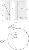 |
Fig. 1 Spectral and geometric relationships for thermal modeling. Top: reflected solar radiance (black curve) and thermally emitted radiance (red curve) emerging from the subsolar point at lunar noon, given a constant reflectance of r = 0.1, an emissivity of e = 0.95 and Adh = 0.07. The spectral domain of the M3 instrument (0.6–3.0 μm) is dominated by solar reflection, but the thermal component increases to the same order of magnitude at 3 μm. The spectral domain of GF-4’s MIR channel (3.5–4.1 μm) is dominated by thermal emission, but roughly 10% of reflected radiance remains. The spectral range of MERTIS (7–14 μm) and Diviner’s channel four (8.10–8.40 μm) are entirely dominated by thermal emission. Bottom: illumination and observation geometry. The shape model is divided into N surface elements. We are interested in the radiance In(λ) that emerges from the nth facet. The vectors s, v, and n indicate the illumination vector, the viewing vector, and the surface normal vector. |
4.2 Observation geometry, shape model, and projection
A planetary shape model consists of N surface elements for each of which we computed the reflected and the thermally emitted light In(λ). Each of these facets is associated with an individual illumination and observation geometry that is commonly expressed by three angles: the incidence angle i between the surface normal n and the illumination vector s, the emission angle e between the surface normal n and the viewing vector v, and the phase angle g between s and v. The thermal roughness model also requires the azimuth angle ψ, measured between the projections of s and v on the tangential plane of the surface. The geometric relations are illustrated in Fig. 1 (bottom). The ground-projected sampling interval (GSI) of the measurements constrains the resolution of the shape model. The GSI of the GF-4 instrument is ≈4 km pixel–1. We chose the LDEM_16ppd (Neumann 2009) from the Lunar Orbiter Laser Altimeter (LOLA) because it has a GSI of <2 km pixel–1 at the equator and hence fulfills Shannon’s sampling theorem. The resolution of the MERTIS observations is coarser, with a GSI of about 500 km pixel–1. Consequently, we lowered the resolution of the simulated lunar disk to about 35 km per pixel, measured at the subspacecraft point. The M3 instrument has a GSI of 140 m pixel–1 (Pieters et al. 2009a), which requires a finer shape model for targeted analyses. Hence, we used the GLD100 (Scholten et al. 2012) refined by the shape from shading procedure of Grumpe & Wöhler (2014). For our global hydroxyl analysis, we downscaled the M3 data such that the GLD100 resolution is sufficient. GF-4 and MERTIS viewed the entire lunar disk from space. Because the distance between the probe and the target was finite, the lunar disk appeared under a perspective projection in the image plane. We modeled this projection with a custom implementation.
4.3 Reflectance model
The models of Hapke (2012) are the current standard for lunar reflectance modeling and form the basis for many photometric (e.g., Warell 2004; Sato et al. 2014), compositional and other surface-related studies (e.g., Wöhler et al. 2017; Wohlfarth et al. 2019; Mustard & Glotch 2019). The model has been repeatedly discussed (Shepard & Helfenstein 2007; Shkuratov et al. 2012), and it does not remain easy to consistently relate the model parameters to the physical characteristics of the regolith. However, Hapke’s approach accurately models the planetary surface’s angular scattering behavior, making it a good choice for our purposes. In this study, the Hapke model enables reflectance normalization, transforms reflectance between various illumination conditions, and is later used to derive the emissivity via the Kirchhoff law (Sect. 4.4) and the directional-hemispherical albedo Adh (Sect. 4.5). The bidirectional reflectance rd relates the solar irradiance to the reflected radiance in a given direction and corresponds to
![Mathematical equation: $\matrix{ {{r_{\rm{d}}}\left( {i,e,g,w} \right) = {w \over {4\pi }}{{{\mu _{0{\rm{e}}}}} \over {{\mu _{0{\rm{e}}}} + {\mu _{\rm{e}}}}}\left\{ {p\left( g \right){B_{S\,H}}\left( g \right) + {L_1}\left( {{\mu _{0{\rm{e}}}}} \right)\left[ {H\left( {{\mu _{\rm{e}}}} \right) - 1} \right]} \right.} \hfill \cr {\quad \quad \quad \quad \quad \,\,\,\, + {L_1}\left( {{\mu _{\rm{e}}}} \right)\left[ {H\left( {{\mu _{0{\rm{e}}}}} \right) - 1} \right] + {L_2}\left[ {H\left( {{\mu _{\rm{e}}}} \right) - 1} \right]} \hfill \cr {\quad \quad \quad \quad \quad \,\,\,\,\, \cdot \left. {\left[ {H\left( {{\mu _{0{\rm{e}}}}} \right) - 1} \right]} \right\}{B_{C\,B}}\left( g \right)S\left( {i,e,g,\bar \theta } \right).} \hfill \cr } $](/articles/aa/full_html/2023/06/aa45343-22/aa45343-22-eq4.png) (2)
(2)
The single scattering albedo w is the fraction of scattered to extinguished radiation by an elementary scatterer and is the dominant model parameter that controls most spectral variations. The model depends on the observation and illumination geometry, expressed by the modified cosines μe = cos(ee) and  and the phase angle g. The phase function p(g) is commonly expressed by the double-lobed Henyey-Greenstein function and is adjusted by the asymmetry parameter b and the weight c. The function BS describes the shadow-hiding opposition effect (SHOE) that is characterized by the amplitude BS0 and width h0. The function S models the shadowing that arises from macroscopic roughness given by the average roughness angle
  . The functions L1, L2, and the Ambartsumian-Chandrasekhar function H are defined in Appendix A. We found it suitable to keep the Hapke parameters fixed to the values given by Warell (2004, see Table 4) and only use the single scattering albedo as a free parameter.
Lunar Hapke parameters according to Warell (2004).
4.4 Emission model
In thermal equilibrium, the solar flux that is not reflected is absorbed and reemitted. Kirchhoff’s law states that the directional emissivity ϵd can be expressed via the hemispherical-directional reflection rhd in thermal equilibrium (Hapke 2012)
 (3)
(3)
In the mid-IR, in which emitted and reflected light are superimposed, it is crucial to accurately account for this relationship as clarified by Myhrvold (2018). The hemispherical-directional reflectance is simply the integral of the bidirectional reflectance rd over the upper half-sphere that collects all incidence directions:
 (4)
(4)
The solution in terms of the Hapke model is given in Appendix A. Due to the integration over half-space, the emissiv-ity varies less with the illumination geometry than the bidirectional reflectance. The emissivity does not change significantly for emission angles below 60°, backed by the empirical studies of Maturilli et al. (2016) and Warren et al. (2019).
4.5 Albedo model
A planetary surface partly reflects and partly absorbs the power carried by the incidence radiation. Only the absorbed component contributes to the planet’s temperature. The bolometric directional-hemispherical albedo Adh quantifies the ratio of the reflected power to the total incidence power such that (1 – Adh) indicates the absorbed power that drives the temperature. The albedo Adh is defined by Shkuratov et al. (2011) and reads
 (5)
(5)
For any given illumination direction, the directional hemispherical reflectance (Eq. (4)) multiplied with the solar spectral irradi-ance E0 provides the hemispherically integrated radiance that is scattered into the upper hemisphere away from the surface. The bolometric integral collects the hemispherically integrated spectral radiance over the entire wavelength range, thus yielding the total reflected power per unit area. Dividing by the solar constant S⊙ leads to the albedo. This definition of Adh is physically sound and depends on the incidence angle i, which is often neglected in cases where no accurate constraints on the directional characteristics are available. We note that the literature provides different albedos used in thermal modeling.
4.6 Thermal model
Planetary surfaces are rough and highly anisothermal. Generally, the thermal emission is not given by a single Planck function but is a superposition of thermal radiation that emerges from many differently oriented facets, each with a different temperature. The resulting thermal spectra may significantly deviate from the thermal emission of a corresponding smooth model (Rozitis & Green 2011; Davidsson et al. 2015). Roughness is responsible for thermal limb brightening and thermal beaming and hence has to be included for adequate thermal modeling. In the case of lunar observations, roughness is essential because it is changes the thermally emitted radiance and the effective brightness temperature, especially near the limb under oblique illumination or viewing conditions. For a thermal roughness model, we adopted the approach of Rozitis & Green (2011), Davidsson et al. (2015), and Rozitis et al. (2020) and extended it to work with fractal surfaces. We opted for fractal surfaces because they most naturally resemble the structure of planetary regolith. Appendix B describes the fractal surface generation method. As described in Sect. 4.2, the first step is to divide the lunar shape model into N surface elements, each of which is denoted by an index n and is associated with an individual illumination and viewing geometry according to Fig. 1 (bottom). The aim is to compute the spectral emission Xn that reaches the sensor for a given surface element n. Therefore, the element n is again subdivided into M smaller facets that build up a rough fractal landscape (Fig. 2 top). The thermal model computes the temperature Tm and the Planck function P(λ, Tm) for each facet m of the fractal. Summing over the Planck functions P(λ, Tm) of the individual facets m yields the spectral emission Xn of the surface element n. In the following section, we describe how to compute Xn and start with the radiation balance of one single fractal facet m. In thermal equilibrium, which is a reasonable assumption given the slow rotation of the Moon, the radiant flux Fm emitted by the mth facet equals the radiant flux brought by the solar light  , scattered radiation
  from neighboring facets, and thermally emitted flux
  from neighboring facets (self-heating):
 (6)
(6)
The geometric relations between these quantities are given in Fig. 2 (bottom). The Stefan-Boltzmann law relates the flux Fm to the temperature of the mth surface element:
 (7)
(7)
where σ is the Boltzmann constant. In the most generic case, the solar flux Jm strikes the surface. The directional-hemispherical albedo Adh controls the fraction of scattered and absorbed radiation. The surface absorbs the majority (1 – Adh) of incoming radiation such that the directly absorbed component  becomes
 (8)
(8)
Here, we assume that the directional-hemispherical albedo Adh is constant for all m within a facet n. The incoming solar irradiance Jm is given by
 (9)
(9)
where S⊙ is the solar constant, rh is the heliocentric distance of the Moon, and im is the incidence angle of the facet. The variable υm is a visibility switch that is either unity if the surface is directly illuminated by the Sun or zero if it is in shadow. The visibility switch is determined via raymarching that uses a variant of the Bresenham algorithm (Bresenham 1965). The surface scatters the remaining part Adh of the incident radiation and reabsorbs a portion of (1 – Adh,m) when the light reaches the surface again. The component  becomes
 (10)
(10)
The viewing factor fm,j determines how much radiation from facet j reaches facet m and is expressed as
 (11)
(11)
Again, υm,j is a boolean value that indicates whether facet m can see facet j and is determined via ray-tracing. We adopted and refined the algorithm of Bresenham (1965) for visibility checks. The mutually projected area of two different surface elements is given by the cosines of the angle between the surface normal and the connection vector between the facets. The angle ϕm is measured between the normal of facet m and the connection vector between facet m and j. The angle ϕj describes the mirrored case and is measured between the normal of facet j and the connection vector between facet m and j. pm,j is the distance between the two facets, and bj is the surface area. This geometry is illustrated in Fig. C.1. However, light can be scattered multiple times. Each scattering iteration corresponds to an additional application of the viewing factors and multiplication with Adh,m, such that  becomes
 (12)
(12)
Parts of the thermal radiation Fm can also heat the surface, known as self-heating. Again, this process occurs repeatedly, such that the contribution  for self-heating becomes
 (13)
(13)
The directional-hemispherical albedo Adh,th of self-heating may not correspond to the value of Adh of the initial scattering process. The directional hemispherical albedos Adh and Adh,th are defined as
 (14)
(14)
 (15)
(15)
where Sth is the thermal emission’s total power per unit area, and X is the spectral emission. Wöhler et al. (2017) and Grumpe et al. (2019) numerically inferred disk-resolved Adh values from M3 measurements, but no such data exist for Mercury. We assume that Adh,th = 0.05, which is a common value in the literature. To solve Eqs. (6)–(13) for the surface temperature Tm, we first move to convenient matrix-vector notation. The components Fm,  and Jm are summarized in the vectors f, fsun, fsca, frad, and j. The viewing factors fm,j are collected in the viewing matrix M such that scattering and self-heating can be expressed through matrix-vector multiplication. The flux balance then becomes
 (16)
(16)
 (17)
(17)
![Mathematical equation: $\matrix{ {{\bf{f}} = \left( {1 - {A_{{\rm{dh}}}}} \right)\underbrace {\left[ {1 + \sum\limits_{k = 1}^\infty {{{\left( {{A_{{\rm{dh}}}}{\bf{M}}} \right)}^k}} } \right]{\bf{j}}}_{{{\bf{d}}_0}}} \cr {\,\,\,\,\,\,\,\,\underbrace { + \left( {1 - {A_{{\rm{dh,th}}}}} \right){\bf{M}}\sum\limits_{k = 0}^\infty {{{\left( {{A_{{\rm{dh,th}}}}{\bf{M}}} \right)}^k}{\bf{f}}} .}_{{{\bf{X}}_{\bf{0}}}}} \cr } $](/articles/aa/full_html/2023/06/aa45343-22/aa45343-22-eq31.png) (18)
(18)
Computing the power of matrix M in d0 and X0 (Eq. (18)) is computationally expensive. Because the spectral norm of M is already small, though, we found it to be sufficient to neglect higher powers of M and introduce the average albedo  , yielding
 (19)
(19)
We rewrote this expression and called for equality. Then the vector f becomes the fixed point of Eq. (20)
 (20)
(20)
If the spectral norm of X is smaller than 1, the iteration rule
 (21)
(21)
converges to the actual value, given an arbitrary start vector (Meister 2015). We chose f0 = d and found that the spectral norm of X is much smaller than one for realistic surface geometries such that convergence is ensured for all practical applications. We found that good convergence is already achieved after five iterations in practically relevant settings. The iteration rule (Eq. (21)) can be rewritten as a sum
 (22)
(22)
It becomes evident that the resulting f scales with (1 – Adh). This fact allowed us to set Adh = 0, precompute only the sum, and later multiply the result with any value for (1 – Adh). Further, one can summarize the vectors d and the resulting f for all N geometric configurations into matrices
![Mathematical equation: ${\bf{F}} = \left[ {{{\bf{f}}_1}{{\bf{f}}_2} \ldots {{\bf{f}}_{\rm{N}}}} \right]\,{\rm{and}}\,{\bf{D}} = \left[ {{{\bf{d}}_1}{{\bf{d}}_2} \ldots {{\bf{d}}_{\rm{N}}}} \right]$](/articles/aa/full_html/2023/06/aa45343-22/aa45343-22-eq37.png) (23)
(23)
and run the iteration for all N geometries simultaneously with
 (24)
(24)
Taking the fourth root of each element of F yields the temperature of the mth facet:
 (25)
(25)
Planck’s radiation law gives the radiation that emerges from the m-th fractal element
 (26)
(26)
and the superposition
 (27)
(27)
yields the final thermal emission component Xn(λ). We found that an edge-width of 200 × 200 pixels is a viable size for the surface fractal, which leads to a 40,000 × 40,000 self-heating matrix. Further, the implementation can be significantly accelerated by subsampling the feature space of geometric combinations. Parameter settings and implementation details for accurate self-heating modeling and accelerated processing are given in Appendix D.
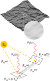 |
Fig. 2 Geometric conventions for the fractal roughness model. Top: simulated fractal surface with M = 200 × 200 elements. The edge width is 1 mm. Bottom: relationship between physical quantities. Adopted from Rozitis & Green (2011). |
4.7 Thermal correction and reflectance normalization for M3 data
For this study, we used the M3 level 1B spectral radiance images available at the Planetary Data System (PDS). The level 2 data were not selected because the thermal correction is known to be incomplete (e.g., Li & Milliken 2017). In order to obtain thermally corrected and normalized reflectance spectra from 0.6 to 3.0 μm, the level 1B M3 data were processed as described by Wöhler et al. (2017) and Grumpe et al. (2019) following four steps. First, an iterative updating scheme was employed to jointly estimate the thermally compensated reflectance rd and the local temperature T. Second, the temperature compensated for roughness effects, so the thermal emission component could be entirely removed. Third, Hapke’s model was employed to photometrically normalize the thermally corrected spectra to the standard geometry (i = 30°, e = 0°, g = 30°). Finally, the calibrated spectra were used to determine the continuum-removed integrated band depth of the 3 μm absorption band, an indicator for surficial OH/H2O. These steps yielded thermally corrected and normalized reflectance spectra. The IBD3μm parameter was introduced by Wöhler et al. (2017) to quantify the average relative absorption strength across the wavelength interval of 2.7–2.9μm
![Mathematical equation: ${{{\rm{IB}}{{\rm{D}}_{3\,{\rm{\mu m}}}} = \left[ {\int_{{\lambda _{\min }}}^{{\lambda _{\max }}} {\left( {1 - {{R\left( \lambda \right)} \over {c\left( \lambda \right)}}{\rm{d}}\lambda } \right)} } \right]} \mathord{\left/ {\vphantom {{{\rm{IB}}{{\rm{D}}_{3\,{\rm{\mu m}}}} = \left[ {\int_{{\lambda _{\min }}}^{{\lambda _{\max }}} {\left( {1 - {{R\left( \lambda \right)} \over {c\left( \lambda \right)}}{\rm{d}}\lambda } \right)} } \right]} {\left[ {{\lambda _{\max }} - {\lambda _{\min }}} \right]}}} \right. \kern-\nulldelimiterspace} {\left[ {{\lambda _{\max }} - {\lambda _{\min }}} \right]}},$](/articles/aa/full_html/2023/06/aa45343-22/aa45343-22-eq42.png) (28)
(28)
where λmin = 2697 nm, λmax = 2936 nm, R(λ) is the bidirectional spectral reflectance, and c(λ) is the linear continuum fitted to the wavelength range of 2537–2657 nm. The absorption strength indicates the amount of surficial OH/H2O, which means that the higher the IBD3μm value, the higher the amount of OH/H2O present.
4.8 Model validation and application
With these methods at hand, we performed four studies for model validation with GF-4 and Diviner data, independent tests for OH/H2O calibration methods with M3 global spectra, and preparation for MERTIS emissivity calibration.
4.8.1 Thermal model validation with GF-4 data
Because band six of the GF-4 satellite stretches from 3.54.1 μm with a center wavelength of 3.77 μm, the measured radiance was subject to approximately 10–20% of reflected solar light. Consequently, we had to employ a combined reflectance and emittance model. We constrained the thermal model with resolved bolometric albedo maps derived from the M3 lunar global mosaic. Because the single-scattering albedo at 3.77 μm cannot be derived directly from the M3 wavelength range, we processed Apollo sample spectra to estimate the albedo and extracted the spectral albedo from around 3.77 μm. We found a robust (r = 0.986) correlation between the albedo at 2.5μm and 3.77μm (see Fig. E.1). Consequently, we applied the linear function to the M3-derived single scattering albedo at 2.5μm and estimated the albedo at 3.77 μm, which was then fed into the reflectance and the emissivity model. The results underwent a perspective projection to match the observation geometry. The optical system of the GF-4 satellite has an unknown point-spread function (PSF) that slightly blurred the target. We assumed a Gaussian PSF and analyzed the expansion of the rim of the lunar disk, which led to σ = 1 pixel. This PSF was applied to the modeled and projected radiance to ensure comparability between the modeled and the measured data. Subsequently, we compared the measured flux of GF-4 with the modeled flux for phase angles of –30.09° and 26.92°. We determined the roughness for mare and highlands, traced the model’s behavior toward the limb, where roughness plays a crucial role, and looked at local variations between different surface areas. Our disk-resolved validation is the first of this kind and complements the validation of Rozitis & Green (2011) and the disk-integrated validation of Müller et al. (2021). As we see later, the modeling results agree exceptionally well with the GF-4 dataset, which justifies applying the model as part of a calibration routine in similar scenarios. We did not consider the case near opposition (g = 3.88°) because the opposition effect is not well understood in this wavelength range, and it remains unclear how these effects can be included without introducing considerable uncertainty, rendering a model validation in the opposition configuration pointless.
4.8.2 Thermal model validation with Diviner nadir and off-nadir data
Thermal emission dominates the spectral region of Diviner channels four (8.25 μm) and seven (25–41 μm) such that solar reflectance becomes negligible. We computed the directional hemispherical reflectance in the NIR and applied Kirchhoff’s law to derive the directional emissivity. In the TIR, the lunarpho-tometric properties are underconstrained such that we refrained from this approach which would require several unknown parameters. Instead, we used a simpler version of the emissivity curve provided by Hapke (2012), which only takes the single scattering albedo as a free parameter. Similar to Bandfield et al. (2015), we did not explicitly resolve the topography but assumed a spherical Moon with small-scale surface roughness. Detailed topographic analysis of the EPF footprint is out of scope for this study but remains an exciting question for future research. The evaluation of the M3 data provided the directional-hemispherical albedo Adh. Consequently, we obtained two free model parameters for each of the eleven EPF maneuvers. We computed the model for 22 roughness values from 19° to 40° with one-degree increments and 51 albedo values from 0 to 0.5 and performed a grid search to find the optimal parameter configuration. Further, we considered Diviner’s observations in nadir pointing. For comparison, we also computed the equilibrium model. We introduced a constant emissivity and scaled the equilibrium temperature to match the rough model brightness temperature near the nadir configuration in the middle of the maneuvers. Bandfield et al. (2015) provided the brightness temperature difference between Diviner channels four and seven, measured at different times of day at specific mare locations. Toward the early morning (06:00) and the evening (18:00), the brightness temperature inferred from channel four becomes up to 70 K higher than channel seven. We derived the directional hemispherical albedo Adh for this scenario, simulated the thermal emission of both channels for three different roughness values ( , 20º, 30º), derived the brightness temperatures, and compared it to Diviner data. Then we analyzed the fitting result and compared it with the GF-4 validation results. Diviner nadir and off-nadir validation extended the mid-infrared model validation with GF-4 data to the thermal infrared domain.
4.8.3 Lunar hydration analysis with the M3 global dataset
We used the TPM for thermal excess correction of lunar NIR reflectance spectra. This calibration process retrieved the 2.8– 3.0 μm absorption band, a measure for surficial OH/H2O, and allowed us to analyze its diurnal, latitudinal, and regional variations. For the calibration, we used the existing processing pipeline for global level 1B data of the M3 instrument (Wöhler et al. 2017; Grumpe et al. 2019) but replaced the old roughness correction with the new thermal roughness model. The calibration pipeline yielded the thermally corrected and normalized reflectance spectra for different lunar times of the day between latitudes of 80º S and 80º N that we uploaded to the supplementary material. Subsequently, we derived global maps of the integrated band depth around 2.8–3.0μm in the lunar morning, midday, and evening, which was the basis for analyzing diurnal, latitudinal, and regional variations. The thermal correction methods of previous studies such as Wöhler et al. (2017), Li & Milliken (2017), Bandfield et al. (2018), and Honniball et al. (2020) have not been tested similarly, and the results did not entirely agree, such that we discussed the previous results in the light of a new thermal model that has proven to be accurate.
4.8.4 Preparations for MERTIS emissivity calibration with lunar flyby data
First, we compared the predicted thermal emission of the lunar disk to the MERTIS measurements acquired on April 9, 2020. MERTIS suffered a slight offset between the nominal and the real pointing direction, which can be corrected as shown by Schmedemann et al. (2021). Further, the instrument’s point spread function (PSF) slightly blurred the emerging radiance and must be considered by the model. We ran a parameter identification routine to fine-tune the pointing offset and match the PSF parameter. This routine minimized the root mean squared error between our radiance model and the measured data. However, our radiance model has a uniform emissivity of one, but the radiance that emerges from the Moon was modulated with the Moon’s unique spectral emissivity spectrum that was not known in advance. Unfortunately, the emissivity resulting from the whole calibration procedure was needed to fine-tune the calibration. To address this coupling of the quantities, we employed an iterative optimization scheme that concurrently estimated the mean spectral emissivity of the lunar disk and the model parameters. Initially, the spectral emissivity was assumed to have a constant value of 0.95, and a Bayesian optimization scheme (Frazier 2018) was employed to retrieve the pointing offset and the width of the PSF. We chose Bayesian optimization because it is well suited to optimize a small set of continuous variables ofa problem that is computationally costly to evaluate. The first iteration then yielded a rough estimate of the parameters. The spectral emissivity was computed and averaged over the whole disk in the next step. The Bayesian optimization was rerun with the updated spectral emissivity. This step yielded an updated parameter set. We ran this iteration for ten cycles and picked the best fit according to the objective function. In this way, we determined the pointing offsets of the MERTIS instrument, which were subsequently transformed into the coordinate system of MERTIS. Finally, the scanned profiles across the lunar disk were compared with the simulated profiles in the four wavelength regions, which is the first observation of a planetary target by MERTIS. We ran the thermal model for 15 roughness values from  and applied the parameter estimation to each.
Secondly, we extended the investigation of Davidsson et al. (2015) to a realistic model of a planetary body to investigate in which cases surface roughness becomes necessary for emissiv-ity retrieval of MERTIS spectra. First, we presented a thermal radiance model of Mercury and traced the effects of surface roughness on the spectral shape for four phase angles of g ≈ 0º, 120º. The topography came from the global digital terrain model of Becker et al. (2009), and the directional hemispherical albedo was inferred from MESSENGER MDIS data as outlined in Appendix F. Further, we sampled the spectral radiance from points near the limb, the middle of the illuminated part, and near the terminator. The spectral radiance of the rough model was then compared to the results of a smooth-surface equilibrium model. We then approximated the spectral radiance of the rough surface by a Planck function. This thermal model will later be used for MERTIS emissivity calibrations of Mercury.
5 Results
5.1 Radiance model for lunar measurements with the GF-4 satellite
This section presents the modeling results of the lunar surface’s combined reflectance and thermal emission at 3.77 µm and compares them to the GF-4 measurements. We independently tested the thermal model, provided accurate roughness estimates, and demonstrated the performance of thermal roughness models. With the insights gained from the validation, we analyzed the thermal model used for the detection of lunar hydration (Sect. 5.3), evaluated the MERTIS flyby measurements (Sect. 5.4.1), and prepared for MERTIS Mercury measurements (Sect. 5.4.2).
5.1.1 The Moon on July 25, 2018
Figure 3 (top) shows the radiance at 3.77 µm, measured on July 25, 2018. The subsolar point is located in the South of Mare Tranquilitatis (white dot in Fig. 3, bottom). The satellite points almost at the center of the lunar disk (black dot in Fig. 3, bottom), spanning a phase angle of −30.09° with the illumination vector. The terminator runs through Oceanus Procellarum, so approximately 93% of the disk is visible. We ran the model for the given geometry and computed the radiance for seven roughness levels ( , 20°, 22°, 24°, 26°, 28°, 30°), averaging over ten random fractal surfaces, respectively. The final result is the weighted superposition of the two roughness levels that best fit the data in the sense of a simple root mean squared error. We assumed linearity, and the average roughness with its 1-sigma error range was inferred to be
  or RMS slope = 22.4098° ± 0.007°. The 1-sigma error range is comparatively small because the number of data points is large, pushing the numerical value down.
The modeled radiance in Fig. 3 (bottom) strongly resembles the measured radiance in Fig. 3 (top). The overall visual appearance is similar, the topographic features match, and the contrast between the mare and highlands has a similar trend. Figure 3 (bottom) indicates horizontal and vertical profile positions for a detailed analysis. The measured and the modeled radiance along the horizontal profiles 25R1–25R4 and the four vertical profiles 25C1–25C4 as given in Fig. 4. The horizontal profiles 25R1–25R4 stretch from the terminator (around pixel position 100–200) to the rim (around pixel position 600–700). A linear slope occurs between the terminator and the subsolar point, and a downturn appears toward the limb (Fig. 4). The vertical profiles 25C1–25C4 nearly stretch from north to south and resemble symmetric arcs (Fig. 4). The modeled and the measured curvatures of horizontal and vertical profiles resemble each other, which indicates that the roughness level is realistic and that the model correctly captures geometry-dependent radiance variations. Profile 25C1 (pixels 400–600), 25C3 (pixels 200–700), and profile 25R4 (pixels 150–600) cover regions with prominent topographic features that lead to abrupt radiance variations. The rough model and the measurements match around these regions, indicating that the underlying topographic model is realistic. The model largely captures the contrast between mare and highland regions. Profile 25R3 exhibits a bump around pixel position 500, which can be associated with the transition between Mare Nectaris and the surroundings mainly consisting of highland material. Profile 25R2 has a plateau-like shape around pixel 500 that stems from Mare Tranquilitatis, also present in profile 25C1 around pixel 300. The prominent notch in profile 25C1 around pixel position 250 results from the transitions between Mare Serenitatis and Sinus Honoris mixed with highland material. However, the model exhibits some deviations. An offset of approximately 1Wm2 sr−1 µm−1 between modeled and measured data occurs for central highland material (see profile 25C2 from pixels 250 to 450 and profile 25R2 around pixel 500 and 600).
 |
Fig. 3 Comparison of the disk-resolved lunar data with the modeling results. Top: radiance I of the lunar disk at 3.77µm measured on July 25, 2018, with the GF-4 satellite. Bottom: radiance of the lunar disk simulated with our model. The arrows indicate the horizontal sampling profiles 25R1–25R4 and the vertical sampling profiles 25C1–25C4. The subsolar point (gray circle) and the subcamera point (black circle) are given in Table 1. |
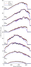 |
Fig. 4 Comparison of the measured radiance (black) with the rough model (red) and the equilibrium model (blue) along the horizontal profiles 25R1–25R4 and along the vertical profiles 25C1–25C4 indicated in Fig. 3 (bottom). Offsets for clarity. |
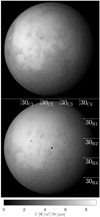 |
Fig. 5 Comparison of the disk-resolved lunar data with the modeling results. Top: radiance I of the lunar disk at 3.77µm measured on July 30, 2018, with the GF-4 satellite. Bottom: radiance of the lunar disk simulated with our model. The dashed lines indicate the horizontal sampling profiles 30R1–30R4 and the vertical sampling profiles 30C1–30C4. The subsolar point (gray circle) and the subcamera point (black circle) are given in Table 1. |
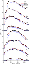 |
Fig. 6 Comparison of the measured radiance (black) with the rough model (red) and the equilibrium model (blue) along the horizontal profiles 30R1–30R4 and along the vertical profiles 30C1–30C4 indicated in Fig. 5 (bottom). Offsets for clarity. |
5.1.2 The Moon on July 30, 2018
Figure 5 (top) shows the radiance at 3.77µm, measured on July 30, 2018. The subsolar point lies in Oceanus Procellarum southwest of Copernicus (white dot in Fig. 5, bottom). The satellite points almost at the center of the lunar disk (black dot in Fig. 5, bottom), spanning a phase angle of 26.92° with the illumination vector. The terminator runs through the area east of Mare Serenitatis and Mare Tranquillitatis, so approximately 95% of the disk is visible. Again, the model was evaluated for seven roughness levels with average slopes of  , 20°, 22°, 24°, 26°, 28°, 30°. The best-fit result with its 1-sigma error range corresponds to a roughness of
  or RMS slope = 23.4763° ± 0.007°.
The modeled radiance in Fig. 5 (bottom) strongly resembles the measured radiance in Fig. 5 (top). The measured and the modeled radiance along the horizontal profiles 30R1–30R4 and the four vertical profiles 30C1–30C4 (see Fig. 5, bottom) is given in Fig. 6. The horizontal profiles appear to be mirrored along the vertical axis, compared to profiles 25R1–25R4 in Fig. 4. Again, the vertical profiles stretch from north to south, resembling a symmetric arc. The model accurately reproduces topographic features (compare profiles 30R4 (pixels 100–600), 30C2 (pixels 500–700), and 30C3 (pixels 500–650)). However, the profiles exhibit slight systematic deviations near the limb. Parts of the modeled profiles 30R1, 30R2, and 30R3 between pixel positions 150–200 are approximately 1Wm2 sr−1 µm−1 below the measured values. The same holds for profile 30C1 for pixels 100–450, which covers the same region. All these profiles cut through a region of Oceanus Procellarum that bears titanium-rich mare material (Lucey et al. 2000). This material is known to be comparatively dark in the visual and infrared, which means the infrared emissivity becomes high. Because there is no accurate emissivity map of the Moon, we extrapolated the albedo and hence Adh and emissivity from M3 measurements to 3.77 µm using Apollo samples. The correlation between the single scattering albedo at 2.50 µm and 3.77 µm (see Sect. 4.5 and Appendix E) is probably not adequate for titanium-rich mare material, such that deviations occur in these regions. A slight difference is also found in profile 25R1, 25R3, and 25C4 but less strong because it is close to the terminator with its comparatively small radiance.
5.2 Radicance model for Diviner’s emission phase function measurements
Our model agrees well with the twelve EPF measurements of Bandfield et al. (2015). Table 5 lists the grid search results for the roughness and the single scattering albedo. The directional hemispherical albedo was derived from the M3 global mosaic.
The average roughness for channel four is around  . The single scattering albedos of both channels are comparatively low, which aligns with the fact that silicate spectra in the thermal infrared have low reflectances and high emissivities. The single scattering albedos of measurements five and six deviate from the rest. The average best-fit roughness of channel seven is similar to channel four, which implies that the model behaves consistently over broader wavelength regions. Appendix G displays the geometries and model results for all twelve EPS measurements (Figs. G.1–G.12) and a lunar topographic map with EPF acquisition locations (Fig. G.13). Because most EPF measurements are similar, we restricted the detailed evaluation to only one representative and one edge case.
Figure 7 (top) shows how the incidence, emission, and azimuth angle develop during the EPF maneuver 11 as explained in Sect. 3. The incidence angle (red) stays largely constant around 46°. The emission angle (blue) and the azimuth angle (black) take nine distinct configurations. The emission angle sucessively takes the values 80°, 72°, 65°, 55°, 0°, 51°, 61°, 67°, 74°. The first four configurations have azimuth angles around 110°, which means that the solar vector and the view vector roughly point in opposite directions. The last four configurations have an azimuth of around 65°, which means that the solar vector and the view vector roughly point into the same half-space.
Figure 7 (bottom) shows the brightness temperature derived from Diviner channel four (red dots) and channel seven (green dots). The data points exhibit a general trend from lower to higher temperatures but scatter strongly, likely due to local albedo and topographic variations. The equilibrium model (solid black) predicts almost constant brightness temperatures around 352 K. Our roughness model (black and blue dots), however, captures the general trend and the stair-like increments of the brightness temperature during the entire maneuver. Our model does not include topography, so it cannot reproduce the local temperature variations. However, the data points scatter symmetrically around the model predictions, which indicates that the model is unbiased. The excellent agreement between diviner EPF measurements and model predictions proves our model accurately simulates how surface roughness impacts the brightness temperature for EPF geometries in the TIR. Figure G.5 shows the brightness temperature of EPF observation number five. The incidence angle rises to i = 69°, and the grid-search result indicates a roughness of  . EPF observation number six (Fig. G.6) covers a nearby region illuminated under i = 67°. However, the best-fit yields
  , which is lower than all other roughness results. There are two possible explanations: Because the observation conditions of EPF observations five and six are similar, it may be true that the roughness at EPF site six is lower than at site five. However, the albedo values strongly differ among themselves and from the rest, which might also indicate that the fitting routine could not sufficiently decouple the roughness and albedo effects at these sites. Tailoring the thermal roughness model to the Diviner EPF data yields average roughness values around
  (RMS slope = 29.61°) for channel four and
  (RMS slope = 28.81°) for channel seven.
The diviner EPF measurements illustrate an essential result of rough surfaces: The TIR brightness temperatures measured under low azimuth angles appear significantly hotter than the equilibrium model. Under high azimuth angles, the brightness temperature appears significantly colder. The brightness temperature is the temperature of the best-fit Planck function that reproduces the radiance measured at a given wavelength interval. Consequently, the brightness temperature of a smooth surface equals its equilibrium temperature. In the case of rough surfaces where each surface facet sustains an individual temperature, the thermal emission is the superposition of the Planck functions of each surface facet. For small azimuth angles (ϕ < 90°), the illumination and the viewing vectors roughly point in the same direction. The spacecraft observes the same facets inclined toward the Sun and obtains higher temperatures. Consequently, their thermal emission is higher than the equilibrium model, and the brightness temperature fit increases. This effect is consistent with thermal limb-brightening and thermal beaming and becomes stronger with increasing emission angle. The illumination and the viewing vectors point to opposite directions for large azimuth angles (ϕ > 90°). The spacecraft primarily observes the facets that face away from the Sun and become colder. At large incidence angles, the rough surface may even exhibit shadows. The spacecraft then observes the colder and the shadowed facets such that the brightness temperature fit yields lower temperatures.
Figure 8 compares the measurements of Bandfield et al. (2015) with our modeling results. Bandfield et al. (2015) find that mare brightness temperatures inferred from nadir observations of channels four and seven differ by time of day. Before 9:00 and after 15:00, the brightness temperature of channel four becomes up to 70 K hotter than channel seven. The brightness temperature difference is marked with black squares. We ran the model for three roughness values. Visual inspection indicates that roughness values close to  (solid red) better describe the brightness temperature anisotropy than
  (dashed red) and
  (dashed-dotted red).
All in all, we reproduced the findings of Bandfield et al. (2015) that the nadir observations are best described by a roughness value close to  (RMS slope 20.89°) and the best fit to model the EPF measurements spans between
  (RMS slope 19.97° – 35.02°) with
  (RMS slope 29.61°) being the mean value for channel four and
  (RMS slope 28.81°) being the mean value for channel seven. Our EPF results are further consistent with other studies in this wavelength range (Rozitis & Green 2011; Bandfield et al. 2015; Rubanenko et al. 2020).
Best fit parameters for twelve EPF measurements of Diviner channels four and seven.
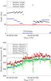 |
Fig. 7 Analysis of EPF measurement no. 11. Top: incidence, emission, and azimuth angle as a function of time during the EPF maneuver. Bottom: brightness temperatures of the Diviner channels four and seven and the modeled brightness temperatures. |
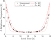 |
Fig. 8 Brightness temperature of Diviner channel four minus channel seven. The measurements (black squares) are taken from Bandfield et al. (2015) and are closest to a thermal model with a roughness of |

5.3 Time-of-day dependent lunar hydration maps
We reprocessed the global level 1B spectral radiance of the M3 instrument with the method of Wöhler et al. (2017) and Grumpe et al. (2019) but with the new thermal roughness model setting the roughness to the rounded average of the GF-4 results ( ). The calibration yields normalized reflectance spectra used to compute the integrated and normalized band depth between 2697 and 2936 nm (IBD3µm). Figure 9 shows global maps of the IBD3µm parameter in the morning, around noon, and in the evening. Three effects can be observed on a global scale. First, there are considerable diurnal variations. In the lunar morning, the IBD3µm parameter is mostly between 8 and 14, with an average of 10.79. The value decreases by 61.74% at noon to 6.66 on average. In the evening, the IBD3µm value increases to 10.51 on average, corresponding to similar levels as in the morning. Secondly, the diurnal variations depend on the region. The amplitude of the diurnal variations is enhanced in the lunar maria, reaching higher IBD3µm values in the morning and evening and lower values around noon. The effect is pronounced in Ti-rich regions, such as western Oceanus Procellarum, central Mare Imbrium, and Mare Tranquilitatis. The amplitude in the lunar highlands is generally lower. On the lunar farside, the diurnal variations in the South Pole-Aitken basin appear to be enhanced compared to the remaining parts. Thirdly, the IBD3µm parameter appears to depend on the latitude. In the morning and evening, the IBD3µm parameter on the lunar farside clearly shows larger values toward the poles compared to the equatorial region and mid-latitudes. This effect can not be entirely separated from regional variations, but on the lunar nearside, the highland-dominated southern quarter exhibits increasing IBD3µm values toward the lunar south pole at all three times of the day. The diurnal variations are the smallest at the highest observed latitudes. We provide the global calibrated reflectance maps for various times of day along with this publication.
5.4 Preparations for MERTIS emissivity calibration
5.4.1 Analysis of MERTIS lunar flyby data
MERTIS’s push-broom-sensor consists of 100 pixels, six of which scanned the lunar disk from the northwest to the southeast through the calibration baffle from an average distance of 725 000 km. The pixel size and the instrument PSF limited the resolution such that the instrument effectively observed an unsharp lunar disk at this distance, as shown in Fig. 10. The yellow lines in Fig. 10 represent the center positions of pixels 36–41 during MERTIS’s scan across the lunar disk after pointing correction. These observation conditions were challenging, and parameter identification appears to be ill-posed. Figure 11 shows the best results from the iterative parameter estimation scheme for each roughness value. The tilts in the east-west (EW) and north-south-direction (NS) of the instrument consistently scatter around ΔWE = −0.19961 mrad and ΔNS = 0.33448 mrad, respectively. The roughness values and the width of the point spread function appear to be correlated. The higher the roughness, the larger the width σ of the Gaussian PSF. Consequently, we did not find an unambiguous minimum, and it was impossible to conclusively determine a single lunar roughness value from MERTIS lunar flyby measurements. Digital optical systems must fulfill Shannon’s sampling theorem such that the full width at half maximum (FWHM) of the PSF equals two pixels. With a pixel size of approximately 500 km, the standard deviation of a Gaussian PSF must be around  . The fitting results are, however, below this value, but given the theory, larger values are more plausible and point to roughness values of about
  . For the highest roughness values, however, the limb appears to be subtly elevated, which might be a hint that the thermal limb-brightening, and thus the roughness value, might be too large. Nevertheless, the fits agree well with the data, and we selected one representative case for
  . Figure 12 shows the measured and radiometrically calibrated radiance profiles across the disk and compares them to the modeled radiance for unit emissivity (dashed red) and the best-fit emissivity (solid red). Pixels at the limb that only partly contain the disk and the deep space are excluded. The rows from top to bottom show the pixels with numbers 36–41. The columns from left to right contain the spectral radiance averaged over the intervals 7.00–8.62µm, 8.79–10.41 µm, 10.59–12.21 µm, and 12.38–14.00µm. The radiance of the unit emissivity model consistently lies above the measured profiles, which indicates that the energy balance is nearly always fulfilled. Only in profile 41_2, the emissivity lies marginally above unity with an estimated value of 1.0025. The best-fit emissivity values range from 0.90 to 1.00. The shortest-wavelength channel has emissivity values from 0.90–0.98 for all profiles. The second channel has almost unit emissivity. The two longest-wavelength channels have consistently low emissivities, mostly between 0.93 and 0.95. The emissivity values are broadly consistent with the emissivity spectra of a silicate mineralogy. The spatial shape of the best-fit model matches the measured radiance, only pixel 37 exhibits a slight but systematic shift to the west. The spectral radiance between the rows varies. The radiance is lowest for the southern and northern profiles 36 and 41, and highest for the center profile 39, whereas the radiance profiles 37, 38, and 40 are in-between. This observation aligns with the trend that the temperature and thermal emission are highest in the disk’s center and decrease toward the limb. See Table 6 for detailed numerical emissivity values.
Emissivity values of six profiles that scanned the lunar disk on April 9th, 2020.
5.4.2 Mercury thermal model simulation
In preparation for future flybys and in-orbit operations, we simulated Mercury for two phase angles of ɡ = 0° and ɡ = 120° and sampled the spectral radiance for unit emissivity at three locations. Mercury’s simulated disk for ɡ = 0° and ɡ = 120° at 5µm is shown in Fig. 13.
Near opposition (ɡ = 0°), the surface roughness leads to higher radiance values at the limb compared to the equilibrium model. Spectrum O_1 in Fig. 13 shows that the rough model predicts radiance values more than twice as high as the smooth surface equilibrium model. Toward the disk’s center, the smooth surface equilibrium and rough models predict nearly identical spectra (spectrum 0_3 in Fig. 13). In this case, a single Planck function of an effective brightness temperature is able to approximate the spectral radiance of the rough-surface model. Between the center and limb of the disk, the rough surface leads to a radiance spectrum that looks slightly enhanced in comparison to a Planck spectrum (spectrum 0_2 in Fig. 13). In addition, enhanced spectral radiance near the limb is the reason for the thermal beaming effect, as discussed by Rozitis & Green (2011).
A large phase angle (ɡ = 120°) leads to a situation in which the smooth surface equilibrium model’s spectral radiance is higher than the rough-surface model's result for most of the visible disk. Near the limb (120_1 in Fig. 14), the spectral shape of the rough-surface model is similar to a Planck function, but near the terminator, the rough spectrum cannot be approximated by a Planck function (120_2 and 120_3 in Fig. 14). These results suggest that different configurations (limb, center, terminator, opposition, near conjunction) lead to complex spectral effects. During a planetary flyby, the MERTIS instrument will scan the disk under various phase angles such that the thermal model must accurately account for these effects. In-orbit operations with oblique incidence angles or off-nadir observations also require this roughness model.
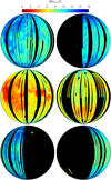 |
Fig. 9 Global IBD3µm map in an orthogonal projection of the lunar nearside (left column) and the lunar farside (right column). Top row: IBD3µm maps in the morning (7:00–8:00). Central row: IBD3µm maps at noon (12:00–14:00 at the nearside and 10:00–12:00 at the farside). Bottom row: IBD3µm maps in the lunar evening (16:00–17:00). Black indicates missing data. |
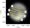 |
Fig. 10 Corrected center positions of MERTIS pixels 36−41 that scanned the lunar disk from west to east. Table 3 gives the subsolar point (gray circle) and the subcamera point (black circle). We applied a Gaussian filter with σ = 300 km to the projected lunar disk to simulate the instrument PSF. |
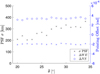 |
Fig. 11 Best fit parameter results for various roughness levels. The optimization scheme consistently retrieves a pointing offset in west-east-direction (ΔWE) and north-south direction (ΔNS). The width of the Gaussian PSF varies with roughness. |
6 Discussion
Validation with Gaofen-4. First, we validated the model with lunar measurements acquired by the GF-4 weather satellite and derived best-fit roughness values. The thermal model generally shows excellent agreement with the GF-4 dataset and accurately describes the radiance at the limb, the dichotomy between maria and highlands, and variations due to topography. Both datasets (July 25 and July 30, 2018) acquired at different phase angles (−30.99° and 26.92°) lead to nearly identical roughness estimates of  and
and  , respectively, which equals an RMS slope of 22.4098° ± 0.008° and 23.4763° ± 0.007°, respectively. The 1-sigma error range is comparatively small because the number of data points is large, pushing the numerical value down.
The first question that naturally arises is what causes slight local deviations between modeled and measured radiance in Figs. 4 and 6. Therefore, we investigated whether we can force fits by varying the roughness parameter or the single scattering albedo. For comparison, we took all seven roughness values from  and introduced a factor that scaled the single-scattering-albedo. The integral (Eq. (14)) weights the reflectance with the solar spectrum and thus suppresses spectral effects in the mid-infrared such that albedo variations around 3.77 µm hardly influence the directional hemispherical albedo and thus we did not need to reprocess Adh. The original model overestimated the radiance around the ejecta blanket of Copernicus (Fig. 6, profile 30R2, Pixel Position 240–360 and Fig. 15 solid black). The smooth equilibrium model with
  (dashed-dotted red Fig. 15) and a rough model with
  hardly deviated from the original model (solid red) and could not provide a good fit. Increasing the single scattering albedo by 50% yielded a good fit. Therefore we conclude that the deviations around Copernicus’s ejecta blanket are likely due to an erroneous albedo estimate with our routine (see Appendix E) that might be caused by the low maturity of the ejecta material. A similar argument holds for the ejecta blanket of Copernicus in profile 30C2 and the highland regions in profiles 30R3, 30C3, 25R2, 25C1, and 25C2 (Figs. 4 and 6).
The original model underestimates the radiance in Oceanus Procellarum that is associated with titanium-rich mare material (Fig. 6, profile 30C1, Pixel Position 100–300 and Fig. 16 solid black line). Even an extremely low single scattering albedo can not provide emissivities that lead to better results (solid blue Fig. 16). Increasing the roughness to around  while keeping the albedo fixed better captures the overall radiance level, but the model still underestimates the radiance in the disk’s center and overestimates the radiance at the limb (dashed red). Only combinations of different effects might accurately explain the radiance profiles. A combination of very low albedo (−90 %) and slightly increased roughness (
 ) yield an adequate fit (dashed-dotted red). Furthermore, we found that reducing the directional hemispherical albedo Adh by 25% and reducing the single scattering albedo by 65% describes the measurements without the need to change the roughness. For Oceanus Procellarum, the parameter identification is ill-posed, and a conclusive evaluation requires more data under multiple geometric configurations that the GF-4 dataset does not provide. After all, it might be the case that the Apollo extrapolation routine (see Appendix E) does not accurately determine the albedo of Ti-rich mare material for the mid-infrared.
All in all, variations of the single scattering albedo can fully explain local deviations around ejecta blankets and bright highland material where the model overestimates the radiance. In Oceanus Procellarum’s titanium-rich regions, only combinations of several effects explain the data, but it is also possible to only alter both albedos to achieve good fits. In any case, these results underline that the roughness varies only slightly, if at all. Thus, the results agree with Bandfield et al. (2015) and partly with Rubanenko et al. (2020), though they find highlands slightly rougher than maria.
Validation with Diviner and MERTIS. A roughness of θ = 20° (RMS slope = 20.90°) best fits the diviner nadir-observations, which agrees with the RMS slope of 20° found by Bandfield et al. (2015). However, eleven out of twelve off-nadir EPF measurements have roughness values around  , (RMS slope = 29.61°) for channel four and
  (RMS slope = 28.81°) for channel seven. One particular case though (Fig. G.6) only requires
  (RMS slope = 19.98°) for the best fit. Because the neighboring EPF measurement (Fig. G.5) exhibits similar geometric configurations and is well described with
  (RMS slope = 27.88°), the deviation of the odd profile might be due to some localized effect. However, it might also be that the fitting routine could not accurately decouple albedo and roughness effects. These overall results agree with Bandfield et al. (2015), who report RMS slopes between 20° and 35° to describe EPF measurements. Other studies such as Rozitis & Green (2011, and references therein) and Rubanenko et al. (2020) also point to values around and above RMS slopes of 30–35°, which is approximately the same value for
  . Due to the challenging observation conditions and underconstrained PSF, a specific roughness value is difficult to obtain from the MERTIS lunar flyby dataset. However, the results tend to be most plausible for values between
  .
.
Surface roughness is a physical property of a planetary regolith that stays constant on geological timescales. Consequently, we must address why the best-fit roughness values differ between GF-4 and Diviner nadir on the one hand and Diviner EPF data on the other hand, even if they all come from the same body and use the same roughness model. Assuming well-calibrated instruments, we discuss three hypotheses explaining the deviations: (1) locally variable roughness, (2) inaccurate model behavior for varying geometric input configurations, and (3) dependence on wavelength.
In principle, the roughness may vary across the lunar surface. However, surface roughness appears to be relatively constant across the lunar surface. In Figs. 3 and 5, one single roughness value leads to model fits that agree with the data in highland and mare regions. There are no systematic deviations toward the limb or the terminator, where roughness effects have the most substantial effect. Only titanium-rich mare regions might exhibit slightly higher values, but the effects can also be due to erroneous albedo extrapolation from Apollo spectra. Bandfield et al. (2015) also report no significant difference and Rubanenko et al. (2020) only report a slight difference between mare and highlands. Even if small roughness variations exist, the differences are not large enough to jump from  to
to  . Consequently, we rule out local deviations as the main culprit for differing roughness values. However, EPF measurements 5 and 6 point to some local roughness deviation (Table 5) that we cannot evaluate further due to the lack of data.
If a thermal model is accurate, it will yield the same roughness value regardless of the geometric input parameter configuration. However, it appears as if the roughness deviations depend on the model’s input geometry. Therefore, we investigated the configuration space spanned by the incidence, emission, and azimuth angles and traced how our six datasets occupy this space (Fig. 17). The geometric configurations of both GF-4 measurements (black) form a surface that approximately takes the shape of a boot. The emission angles of nadir measurements vanish by definition (e = 0°), but the incidence and azimuth angles can take arbitrary values (i = 0… 90°, ϕ = 0… 180°). Consequently, nadir measurements occupy a plate in the configuration space (green circles) where the Diviner nadir data form a subset. The EPF measurements (red points) observe the Moon under oblique emission angles over a wide range of azimuth angles. The incidence angle remains around i ≈ 60°. Most geometric configurations of the global M3 dataset have e < 30°, but they span almost the entire azimuth and emission angle range. The geometric configuration of MERTIS measurements is very close to both GF-4 datasets, such that the point clouds are indistinguishable. The point clouds of Diviner nadir measurements ( ) and GF-4 (
 ) partially overlap. The geometric configurations of the Diviner EPF measurements (
 ) lie outside of the other datasets at a different region of the configuration space (see Fig. 17). Saari et al. (1972) measured parts of the sunlit portion of the Moon over a whole lunation such that the parameter configurations occupy a similar region to the Diviner EPF measurements. Rozitis & Green (2011) used this lunation dataset for roughness model validation, leading to an RMS slope of 31.5° ± 1.5° and 33.0° ± 1.1°. The same holds for the lunar phase curve observations of Müller et al. (2021), which are best described with a roughness around 32°. This analysis suggests that the roughness fits deviate between datasets taken under different geometric configurations. Nadir-like or frontal disk observations yield roughness values around
  , while the EPF measurements and other phase curve observations yield
  . Consequently, our observation suggests that our roughness model, and probably similar approaches, may not be accurate for all geometric input configurations.
Future research should therefore identify and improve the inexact model components. Two candidates may be the roughness type and the emissivity model. Davidsson et al. (2015) discuss that the roughness type partially controls the anisotropic behavior of thermal models. However, we already used rough fractal surfaces, theoretically the most realistic representation of lunar regolith. The behavior at thermal isolation scales may yield further insights, requiring a small-scale three-dimensional heat-transfer model. Most studies assume a constant isotropic emissivity of ϵ ≈ 0.90–0.95 that does not depend on the emission angle. However, the emissivity is anisotropic. Few works provide emissivity models, but Hapke’s theory predicts that a horizontally stratified medium emits less radiation as the emission angle increases (Hapke 2012). The higher the surface albedo, the stronger the effect. Therefore, the anisotropic emission superimposes the anisotropic effects of surface roughness, which changes the overall model behavior. An alternate approach is determining the surface reflectance and inferring the emissivity via Kirchhoff’s law. However, lunar reflectance might not be constrained entirely, which adds further uncertainty. We addressed anisotropic emissivity effects in our model. In retrospect, we evaluated whether the emissivity model may have caused model variations that are strong enough to explain the differences between GF-4 and Diviner roughness estimates but did not find significant evidence. Diviner channel four is around the Christiansen feature, such that the emissivity is already close to unity, and the single scattering albedo almost vanishes (Table 5). In this case, the Hapke emissivity model hardly predicts anisotropic variations (see Hapke 2012), which further holds for the Kirchhoff approach. In the case of the GF-4 measurements, the single scattering albedo is higher, and the emissivity effect increases. However, the emissivity model yields decreasing emissivity values toward the limb of the disk, while the roughness model counteracts and predicts increasing thermal emission. Removing the emissivity model even leads to slightly smaller roughness values. Consequently, the emissivity model would have to decrease toward higher emission angles for higher roughness values. Further, the emissivity depends on the wavelength and may exhibit different behaviors for spectral regions near the Christiansen feature around 8 µm compared to the near- and mid-infrared. Wavelength dependence might explain why the GF-4 data are better matched with  , while the MERTIS data are better described by higher roughness, though their geometric configuration is quite similar (Fig. 17).
Better understanding the role of the emissivity model requires more theoretical work. The Hapke model is based on radiative transfer for horizontally stratified homogeneous media. The roughness models simulate individual facets of a rough regolith, which might be incompatible on a theoretical level. Warren et al. (2019) present a promising approach in which they numerically compute the emissivity of a rough isothermal surface and validate the results with a goniometer setup. However, the approach has yet to be extended to anisothermal scenarios and must undergo more extensive validation with regolith material.
Lunar hydration. We reprocessed the global level 1B spectral radiance of the M3 instrument with the method of Wöhler et al. (2017) and Grumpe et al. (2019) but with the new thermal model, setting the roughness to the rounded average of the GF-4 results of  . The following three observations back this choice. First, the GF-4 measurements are in a similar wavelength region compared to the long-wavelength end of M3 and should exhibit similar behavior. Second, Diviner nadir measurements point to roughness values around
  and lie in a similar region of the configuration space. Third, GF-4 and M3 data partially overlap in the configuration space. Consequently, GF-4 and Diviner nadir measurements sufficiently constrain the M3 data. The value of
  is similar to the previous roughness estimate of
  (Wöhler et al. 2017; Grumpe et al. 2019) and the average lunar roughness (20° RMS slope) used by Bandfield et al. (2015, 2018). The alternative solution in Wöhler et al. (2017) and Grumpe et al. (2019) of
  , however, appears to be too smooth.
The updated results align well with other studies, such as Honniball et al. (2020), who reported diurnal and latitudinal variations using an entirely different dataset obtained with the ground-based SpeX instrument. Honniball et al. (2020) also found a dichotomy with higher OH/H2O abundances in the highland regions, which corresponds to the original findings of Wöhler et al. (2017) and Grumpe et al. (2019) and to our new results for lunar midday. However, Honniball et al. (2020) did not carry out detailed emissivity and albedo modeling. Laferriere et al. (2022) recently reevaluated data from the Deep Impact spacecraft and found that lunar OH/H2O is widespread but variable across the lunar south pole. Except for the lowest temperatures, highlands have stronger absorption bands than mare regions, which aligns with our maps at lunar midday. For low temperatures in the morning and evening, we find that maria have a slightly stronger hydration feature than highlands, which does not contradict Laferriere et al. (2022). Hence, our results largely agree with two independent datasets (SpeX and Deep Impact), which strongly suggest the widespread presence and the diurnal and latitudinal variations of lunar hydration. The observations may be explained by an exospheric process in which solar wind implantation of protons induces an accumulation of lunar OH/H2O during the morning and afternoon, whereas thermal evaporation and photolysis lead to a depletion during midday (Grumpe et al. 2019; Schörghofer et al. 2021).
MERTIS lunar flyby. The conditions under which MERTIS observed the Moon were challenging, as it had to acquire the data through the calibration baffle. The distance between the Moon and the instrument was large, so only six pixels scanned the lunar disk. Further, the Moon is much colder than Mercury, and consequently, the TIR emission is approximately ten times smaller than the emission expected for Mercury. Due to the resulting low signal-to-noise ratio, we binned the lunar flyby data into four broad wavelength channels. We generally find a good match between the modeled radiances and the measured radiance profiles across the disk. However, we cannot provide a precise roughness results because of the point spread function.
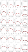 |
Fig. 12 Radiance profiles for pixel 36–41 over four integrated wavelength channels, 7.00–8.62 µm, 8.79–10.41 µm, 10.59–12.21 µm, 12.38–14.00 µm. |
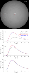 |
Fig. 13 Simulated Mercury disk for a phase angle of ɡ = 0°. The plots show the spectral radiance at the indicated locations. |
 |
Fig. 14 Simulated Mercury disk for a phase angle of ɡ = 120°. The plots show the spectral radiance at the indicated locations. |
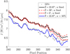 |
Fig. 15 Measured radiance (points) around crater Copernicus vs. various modeling approaches (solid lines). The data points correspond to a subsample of profile 30R2 in Fig. 6. Adjusting the single scattering albedo w leads to a better agreement. |
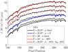 |
Fig. 16 Measured radiance (points) across a titanium-rich region of Oceanus Procellarum vs. various modeling approaches (solid lines). The data points correspond to a subsample of profile 30C1 in Fig. 6. To avoid clutter, we offset the profile groups by 1 W m−2 sr−1 µm−1. |
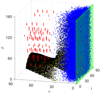 |
Fig. 17 Configuration space is spanned by the incidence angle i, the emission angle e, and the azimuth angle ϕ. The data points represent the geometric configurations associated with the measurements used throughout this study. Black: lunar measurements by GF-4 on July 25, 2018, and July 30, 2018. Green: Diviner nadir measurements lie in this plane. Red: Diviner EPF measurements. Blue: M3 global dataset. Yellow: MERTIS lunar flyby. To avoid clutter, we subsampled the GF-4, M3, and MERTIS data points. |
7 Conclusion
This study presented, validated, and applied a combined reflectance and thermal emission model for airless planetary bodies. The thermal model comprises rough fractal surfaces, self-heating, self-scattering, and realistic albedos. The matrix-vector formalism and the numerical implementation accelerate the computation time such that the model can process entire planetary disks with all effects on fractal surfaces.
First, we validated the model with lunar measurements acquired by the Gaofen-4 weather satellite and the Diviner lunar radiometer. GF-4 measured the disk-resolved Moon in the infrared around 3.77 µm, providing two lunar disks under phase angles of −30.99° and 26.92°, respectively. The radiances resulting from our model and the measured radiances agree nearly exactly in most parts of the lunar disk. However, slight deviations occur in regions associated with titanium-rich mare material and brighter regions, such as the ejecta blanket of Copernicus. Both cases might be explained by undercon-strained single scattering albedo input for this composition. The best-fit roughness parameters are  (July 25, 2018) and
  (July 30, 2018), which equals an RMS slope of 22.4098° ±_0.008° and 23.4763° ± 0.007°, respectively. A roughness of
  well approximates Diviner nadir observations. To match the Diviner EPF measurements, roughness values from
  are necessary with an average around
  . The roughness derived from the EPF measurements agrees with the work of Bandfield et al. (2015) and other studies such as Rozitis & Green (2011), Rubanenko et al. (2020), and Müller et al. (2021). Even though the modeling results are internally consistent, we find systematic deviations between GF-4 and nadir measurements on the one hand and Diviner EPF data on the other hand. This result is also comparable to Bandfield et al. (2015). We discuss various reasons and conclude that the anisotropic emissivity deviates depending on the geometry and the wavelength. This finding calls for more theoretical and laboratory work to provide more realistic emissivity models in the future.
Second, we used the new thermal model to reprocess the M3 radiance measurements of the lunar surface to analyze the 2.8–3.0 µm absorption band that indicates the presence of surficial OH/H2O. We showed that a roughness value of  is realistic for the M3 wavelengths and configurations. The results clearly show the diurnal variations of the integrated band depth of the 3 µm absorption band. The updated results show more clearly the latitudinal variations with deeper absorption bands toward the lunar poles, which agrees with recent studies (e.g., Honniball et al. 2020 and Laferriere et al. 2022). The dichotomy between mare and highland is also visible, where the diurnal amplitude appears stronger for maria than for highlands.
Third, we compared our thermal modeling results to lunar measurements at 7–14 µm that MERTIS acquired during a swing-by maneuver. The modeled radiance agrees with how the measured radiance changes across the lunar disk. However, near the resolution limit, we had to consider the effects of a point spread function, which led to an ill-posed problem but provided accurate fits that conform with roughness values between  . Due to observational constraints, we limited the spectral resolution to four broad channels. The emissivity values in these channels are consistent with the emissivity spectra of a silicate mineralogy.
Fourth, we simulated the thermal emission for Mercury under phase angles of 0° and 120°. This simulation points out the cases in which the thermal roughness model deviates most strongly from smooth thermal models and a single Planck function. In opposition configuration, the thermal limb brightening becomes evident because the facets tilted toward the Sun are also tilted toward the observer. The limb thus appears hotter than predicted by a smooth model. At large phase angles, the observer sees more shadows which makes the surface seem colder. In both configurations, the simulated thermal emission does not follow a single Planck function anymore. These effects will be further investigated for Mercury with BepiColombo.
Acknowledgements
This work has partially been funded by the German Aerospace Center (DLR), FKZ 50QW2201B. We would also like to thank an anonymous reviewer whose comments enhanced the quality of the study.
Appendix A Hapke model
The bidirectional reflectance of the Hapke model (Hapke 2012) corresponds to
![Mathematical equation: $\matrix{ {{r_{\rm{d}}}\left( {i,e,g,w} \right) = {w \over {4\pi }}{{{\mu _{0,{\rm{e}}}}} \over {{\mu _{0,{\rm{e}}}} + {\mu _{\rm{e}}}}}\left\{ {p\left( g \right){B_{SH}}\left( g \right) + {L_1}\left( {{\mu _{0,{\rm{e}}}}} \right)\left[ {H\left( {{\mu _{\rm{e}}}} \right) - 1} \right]} \right.} \cr {\quad \quad \quad \,\,\, + {L_1}\left( {{\mu _{\rm{e}}}} \right)\left[ {H\left( {{\mu _{{\rm{0,e}}}}} \right) - 1} \right] + {L_2}\left( {{\mu _{\rm{e}}}} \right)\left[ {H\left( {{\mu _{\rm{e}}}} \right) - 1} \right]} \cr {\left. { \cdot \left[ {H\left( {{\mu _{{\rm{0,e}}}}} \right) - 1} \right]} \right\}{B_{CB}}\left( g \right)S\left( {i,e,g,\bar \theta } \right).} \cr } $](/articles/aa/full_html/2023/06/aa45343-22/aa45343-22-eq103.png) (A.1)
(A.1)
Here, µ0,e and µe are the modified cosines of the incidence and the emission angle, respectively. The quantity w is the single-scattering albedo. The function p(ɡ) is termed the phase function and depends on the phase angle ɡ between the illumination direction and the viewing direction. It is expressed by the double-lobed Henyey-Greenstein (DHG) function. The Ambartsumian-Chandrasekhar H-function cannot be expressed analytically. Following Hapke (2012), it is approximated by
![Mathematical equation: $H\left( x \right) = {\left\{ {1 - wx\left[ {{r_0} + {{1 - 2{r_0}x} \over 2}\ln {{1 + x} \over x}} \right]} \right\}^{ - 1}},$](/articles/aa/full_html/2023/06/aa45343-22/aa45343-22-eq104.png) (A.2)
(A.2)
where
 (A.3)
(A.3)
 (A.4)
(A.4)
The remaining terms for L1 and L2 are defined by:
 (A.5)
(A.5)
 (A.6)
(A.6)
 (A.7)
(A.7)
The coefficients bn follow from the Legendre series expansion of the double-lobed Henyey Greenstein function. The coefficients An are calculated recursively:
 (A.8)
(A.8)
 (A.9)
(A.9)
Appendix B Fractal surface generation
We used a spectral synthesis method that generates fractional Brownian motion representing the rough lunar regolith. Saupe (1991) outlines the theoretical approach of Fourier-based algorithms, and the authors of Grumpe et al. (2019) wrote the initial implementation for this study. They averaged over the RMS slope angle statistics shown in Figure 9 of Helfenstein & Shepard (1999). The resulting RMS-slope statistic set our reference. We then scaled the RMS slope angle of the reference fractal statistics up and down to generate smoother or rougher surfaces. The observationthatthe RMSslope statistic ofsmootherandrougher planetary regolith can be converted by simple multiplication supports our approach. We realized ten different fractals drawn from the scaled RMS-slope input statistics for each roughness level and computed the corresponding thermal models. Finally, we average over the resulting thermal emission to even out directional effects that stem from individual realizations of the fractal surface.
Appendix C Geometric relations for the thermal model
Figure C.1 sketches the geometric relations for self-heating and self-scattering between two thermally isolated facets m and j of one fractal surface. The Sun has a distance of rh to the entire scene and illuminates the surface with irradiance S0. The self-heating (and self-scattering) coefficients fm,j indicate how much radiation facet m receives from facet j and vice versa
 (C.1)
(C.1)
The angle ϕm is measured between the normal vector Zm of facet m and the vector that connects the center of facet m with facet j. The angle ϕj is measured between the normal vector Zj of facet j and the vector that connects the center of facet j with facet m. pm,j is the distance between both facets.
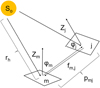 |
Fig. C.1 Geometric relations for self-heating and self-scattering. |
Appendix D Implementation Details
Subsampling ofparameterspace: Even foramoderate discretization of the lunar surface, the number of geometric configurations N becomes very large. The GF-4 measurement of July 25, 2018, contains about360,000 pixels. Running the model forten fractals with a size of 200 × 200 pixels for each surface element results in 144 billion operations. Each operation encompasses self-heating and visibility analysis, making the total problem impractical. However, analyzing the mathematical structure ofthe geometries yields a way to decouple the computational effort of the thermal model from the initial problem size. This step dramatically reduces the total computational burden. For illumination and viewing vectors, we found that all geometric configurations lie on a continuous manifold within a space spanned by the geometry parameters i, e, and ψ. We found that it suffices to sample the manifold and compute the thermal model via equation 24 for only several thousand points in this parameter space. We further exploited equation 22 and precomputed the model for Adh = 0 and later scaled it to the desired values. Simple linear interpolation between sample points suffices to reconstruct a scene of arbitrary size. This approach drastically reduced the computational effort, such that the model now finishes within several hours on an AMD EPYC 7742 CPU. This approach is illustrated in Figure D.1 (top).
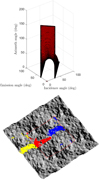 |
Fig. D.1 Geometrie conventions for computational techniques that speed up the thermal model computation. Top: The red surface represents all geometric configurations of the angles i, e, and ψ that describe the lunar surface seen by GF-4 on July 25, 2018. The black dots indicate the sampling points we evaluate the thermal model. Bottom: Example for self-heating on periodic fractal surfaces. A red square encircles the original fractal surface of 200 × 200 pixels. Outside the red square, it is repeated periodically. A white X marks the pixel of interest. The red pixels within the red square directly illuminate X for a given self-heating radius of 100 pixels. When assuming periodicity, the blue pixels within the original fractal are transported to the yellow pixel positions. Now, X receives a realistic amount of self-heating radiation, even though it is located at the edge of the original fractal surface. |
Periodicity for efficient self-heating: Self-heating and self-scattering consider the power the current surface facet receives from its neighbors. We must collect all contributions from the neighborhood, to fulfill energy conservation. Ideally, this neighborhood would be infinite, but the contributions rapidly get smaller with increasing distance. Because the computational complexity grows quadratically with the size of the neighborhood, it is helpful to limit the neighborhood by introducing a self-heating radius. We found that at a radius of 100 pixels collects 95% of self-heating and self-scattering radiation while keeping the computational complexity reasonable. However,
facets near the edge or in the corners of a rectangular fractal receive less radiation via self-heating, which leads to an underestimation of their temperature. Enlarging the fractal surface and neglecting the edges would alleviate the issue but is computationally expensive. A more efficient way is to exploit the properties of the fractal generation algorithm, which is based on the Fourier transform. The fractal landscape is periodically continuous, which means that opposite edges of the fractal surface are identical (gluing the left and the right edge together would result in a cylinder with a seamless transition). This property allows us to compute the self-heating over the edges and collect an adequate amount of self-heating radiation even for pixels near the edge. We set the fractal surface to 200 × 200 pixels and define a self-heating area of 100 × 100 pixels. An example is given in Figure D.1 (bottom).
Appendix E Albedo estimation from RELAB data
Figure E.1 shows the correlation between the single scattering albedo of the Apollo samples measured at 2500 nm and 3770 nm. The reflectance spectra are taken from the RELAB database. The albedos are inferred via the Hapke model. The Highland samples (blue) are brighter compared to the Mare samples. We found a linear correlation between the albedo at both wavelength channels, which helped to extrapolate the albedo in the GF-4 wavelength range given the M3 global mosaic.
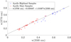 |
Fig. E.1 Correlation between the single-scattering albedo at 2500 nm and 3770 nm for Apollo samples. |
Appendix F Directional-hemispherical albedo for Mercury
According to equation 5, the directional hemispherical albedo is the bolometric integral over the directional hemispherical reflectance weighted with the solar spectrum. Consequently, the value for Adh is primarily controlled by the reflectance from the ultraviolet to the mid-infrared. Currently, no reflectance spectra are available that cover a spectral region that is broad enough to directly compute the directional hemispherical albedo of Mercury. However, it is possible to establish an empirical relationship that robustly predicts the directional hemispherical albedo Adh given the incidence angle i and the single scattering albedo w at 750 nm. Therefore we assume a two-dimensional polynomial of the form
 (F.1)
(F.1)
We insert i, w, and Adh as computed for the lunar observation on July 25, 2018, and estimate the coefficients a0–a5 with Least-squares. We choose a wavelength of 750 nm for the albedo because it is not affected by spectral absorption bands. The Moon
and Mercury have silicate mineralogies, so the overall spectral shapes are roughly comparable. Direct comparison shows that the reflectance spectra of Mercury are featureless in the near-infrared and approximately as dark as the lunar maria. Because the bolometric integral mainly depends on the overall spectral shape, we assume that the empirical relationship inferred for the lunar surface also holds for Mercury. Consequently, we derive the single scattering albedo from the MDIS global mosaic at 750 nm and then estimate Adh for Mercury.
Appendix G Diviner Emission Phase Function Results
This section displays the results of our thermal model compared with the EPF measurements for all 12 EPF measurements. Table 2 provides the observation conditions, and Table 5 lists the fitting results for the single scattering albedo w and the roughness  .
.
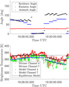 |
Fig. G.1 EPF maneuver 1. Top: Geometry. Bottom: Modeled vs. measured brightness temperatures. |
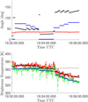 |
Fig. G.2 EPF maneuver 2. Top: Geometry. Bottom: Modeled vs. measured brightness temperatures. |
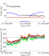 |
Fig. G.3 EPF maneuver 3. Top: Geometry. Bottom: Modeled vs. measured brightness temperatures. |
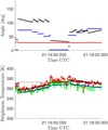 |
Fig. G.4 EPF maneuver 4. Top: Geometry. Bottom: Modeled vs. measured brightness temperatures. |
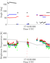 |
Fig. G.5 EPF maneuver 5. Top: Geometry. Bottom: Modeled vs. measured brightness temperatures. |
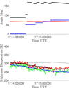 |
Fig. G.6 EPF maneuver 6. Top: Geometry. Bottom: Modeled vs. measured brightness temperatures. |
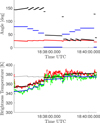 |
Fig. G.7 EPF maneuver 7. Top: Geometry. Bottom: Modeled vs. measured brightness temperatures. |
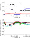 |
Fig. G.8 EPF maneuver 8. Top: Geometry. Bottom: Modeled vs. measured brightness temperatures. |
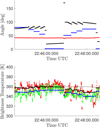 |
Fig. G.9 EPF maneuver 9. Top: Geometry. Bottom: Modeled vs. measured brightness temperatures. |
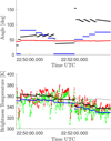 |
Fig. G.10 EPF maneuver 10. Top: Geometry. Bottom: Modeled vs. measured brightness temperatures. |
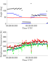 |
Fig. G.11 EPF maneuver 11. Top: Geometry. Bottom: Modeled vs. measured brightness temperatures. |
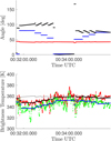 |
Fig. G.12 EPF maneuver 12. Top: Geometry. Bottom: Modeled vs. measured brightness temperatures. |
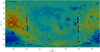 |
Fig. G.13 Lunar topographic map with all 12 EPF measurements listed in Table 2. White numbers indicate the EPF measurement counted from first to last. Red lines indicate the subspacecraft point. Black stars show the locations of the measurements. |
References
- Bandfield, J. L., Hayne, P. O., Williams, J.-P., Greenhagen, B. T., & Paige, D. A. 2015, Icarus, 248, 357 [Google Scholar]
- Bandfield, J., Poston, M., Klima, R., & Edwards, C. 2018, Nat. Geosci., 11, 173 [NASA ADS] [CrossRef] [Google Scholar]
- Bauch, K. E., Hiesinger, H., Helbert, J., Robinson, M. S., & Scholten, F. 2014, Planet. Space Sci., 101, 27 [NASA ADS] [CrossRef] [Google Scholar]
- Bauch, K. E., Hiesinger, H., Greenhagen, B. T., & Helbert, J. 2021, Icarus, 354, 114083 [NASA ADS] [CrossRef] [Google Scholar]
- Becker, K. J., Robinson, M. S., Becker, T. L., et al. 2009, AGU Fall Meeting Abstracts, 2009, 1189 [Google Scholar]
- Bresenham, J. E. 1965, IBM Syst. J., 4, 25 [Google Scholar]
- Buhl, D., Welch, W. J., & Rea, D. G. 1968, J. Geophys. Res., 73, 5281 [CrossRef] [Google Scholar]
- Capria, M. T., Tosi, F., De Sanctis, M. C., et al. 2014, Geophy. Res. Lett., 41, 1438 [NASA ADS] [CrossRef] [Google Scholar]
- Christensen, P. R., Hamilton, V. E., Mehall, G. L., et al. 2018, Space Sci. Rev., 214, 87 [Google Scholar]
- Clark, R. N. 1979, Icarus, 40, 94 [NASA ADS] [CrossRef] [Google Scholar]
- Clark, R. N. 2009, Science, 326, 562 [NASA ADS] [CrossRef] [Google Scholar]
- Clark, R. N., Pieters, C. M., Green, R. O., Boardman, J. W., & Petro, N. E. 2011, J. Geophys. Res. Planets, 116, 2010JE003751 [Google Scholar]
- Coradini, A., Capaccioni, F., Drossart, P., et al. 2007, Space Sci. Rev., 128, 529 [Google Scholar]
- Davidsson, B. J., Rickman, H., Bandfield, J. L., et al. 2015, Icarus, 252, 1 [CrossRef] [Google Scholar]
- Delbo, M., Mueller, M. P. E. J., Rozitis, B., & Capria, M. T. 2015, in Asteroids IV, eds. P. Michel, F. E. Demeo, & W. F. Bottke (Tucson: The University of Arizona Press), 107 [Google Scholar]
- Denevi, B. W., Ernst, C. M., Prockter, L. M., & Robinson, M. S. 2018, in Mercury: The View after MESSENGER, eds. S. C. Solomon, L. R. Nittler, & B. J. Anderson, Cambridge Planetary Science (Cambridge: Cambridge University Press), 144 [Google Scholar]
- De Sanctis, M. C., Coradini, A., Ammannito, E., et al. 2012, in The Dawn Mission to Minor Planets 4 Vesta and 1 Ceres, eds. C. Russell, & C. Raymond (New York, NY: Springer New York), 329 [Google Scholar]
- Emery, J., Sprague, A., Witteborn, F., et al. 1998, Icarus, 136, 104 [NASA ADS] [CrossRef] [Google Scholar]
- Frazier, P. I. 2018, ArXiv e-prints [arXiv:1807.02811] [Google Scholar]
- Grumpe, A., & Wöhler, C. 2014, ISPRS J. Photogramm. Remote Sens., 94, 37 [Google Scholar]
- Grumpe, A., Wöhler, C., Berezhnoy, A., & Shevchenko, V. 2019, Icarus, 321, 486 [NASA ADS] [CrossRef] [Google Scholar]
- Hapke, B. 2012, Theory of Reflectance and Emittance Spectroscopy, 2nd edn. (Cambridge: Cambridge University Press) [Google Scholar]
- Harris, A. W. 1998, Icarus, 131, 291 [Google Scholar]
- Hayne, P. O., Bandfield, J. L., Siegler, M. A., et al. 2017, J. Geophys. Res. Planets, 122, 2371 [Google Scholar]
- Helfenstein, P., & Shepard, M. K. 1999, Icarus, 141, 107 [Google Scholar]
- Hiesinger, H., & Helbert, J. 2010, Planet. Space Sci., 58, 144 [NASA ADS] [CrossRef] [Google Scholar]
- Hiesinger, H., Helbert, J., Alemanno, G., et al. 2020, Space Sci. Rev., 216, 147 [CrossRef] [Google Scholar]
- Honniball, C. I., Lucey, P. G., Ferrari-Wong, C. M., et al. 2020, J. Geophys. Res. Planets, 125, e2020JE006484 [Google Scholar]
- Keihm, S. J., & Langseth, M. G. J. 1973, Lunar Planet. Sci. Conf., 4, 2503 [Google Scholar]
- Laferriere, K. L., Sunshine, J. M., & Feaga, L. M. 2022, J. Geophys. Res. Planets, 127, e2022JE007361 [CrossRef] [Google Scholar]
- Lagerros, J. S. V. 1996, A&A, 310, 1011 [Google Scholar]
- Lebofsky, L. A., Veeder, G. J., Lebofsky, M. J., & Matson, D. L. 1978, Icarus, 35, 336 [NASA ADS] [CrossRef] [Google Scholar]
- Lebofsky, L. A., Sykes, M. V., Tedesco, E. F., et al. 1986, Icarus, 68, 239 [NASA ADS] [CrossRef] [Google Scholar]
- Li, S., & Milliken, R. E. 2016, J. Geophys. Res. Planets, 121, 2081 [NASA ADS] [CrossRef] [Google Scholar]
- Li, S., & Milliken, R. E. 2017, Sci. Adv., 3, e1701471 [Google Scholar]
- Lucey, P. G., Blewett, D. T., & Jolliff, B. L. 2000, J. Geophys. Res. Planets, 105, 20297 [CrossRef] [Google Scholar]
- MacLennan, E. M., & Emery, J. P. 2018, AJ, 157, 2 [NASA ADS] [CrossRef] [Google Scholar]
- Marshall, D., Groussin, O., Vincent, J.-B., et al. 2018, A&A, 616, A122 [NASA ADS] [CrossRef] [EDP Sciences] [Google Scholar]
- Maturilli, A., Helbert, J., Ferrari, S., & D’Amore, M. 2016, Earth, Planets and Space, 68 [Google Scholar]
- McCoy, T. J., Peplowski, P. N., McCubbin, F. M., & Weider, S. Z. 2018, in Mercury: The View after MESSENGER, eds. S. C. Solomon, L. R. Nittler, & B. J. Anderson, Cambridge Planetary Science (Cambridge: Cambridge University Press), 176 [Google Scholar]
- Meister, A. 2015, Numerik linearer Gleichungssysteme (Wiesbaden: Springer Spektrum) [CrossRef] [Google Scholar]
- Müller, T. G., Burgdorf, M., Alí-Lagoa, V., Buehler, S. A., & Prange, M. 2021, A&A, 650, A38 [NASA ADS] [CrossRef] [EDP Sciences] [Google Scholar]
- Mustard, J. F., & Glotch, T. D. 2019, in Remote Compositional Analysis: Techniques for Understanding Spectroscopy, Mineralogy, and Geochemistry of Planetary Surfaces, eds. J. L. Bishop, J. F. Bell III, & J. E. Moersch, Cambridge Planetary Science (Cambridge: Cambridge University Press), 21 [Google Scholar]
- Myhrvold, N. 2018, Icarus, 303, 91 [Google Scholar]
- Neumann, G. 2009, Lunar Orbiter Laser Altimeter Raw Data Set, online; accessed January 27, 2022 [Google Scholar]
- Okada, T., Fukuhara, T., Tanaka, S., et al. 2018, Planet. Space Sci., 158, 46 [Google Scholar]
- Paige, D. A., Foote, M. C., Greenhagen, B. T., et al. 2010a, Space Sci. Rev., 150, 125 [Google Scholar]
- Paige, D. A., Siegler, M. A., Zhang, J. A., et al. 2010b, Science, 330, 479 [NASA ADS] [CrossRef] [Google Scholar]
- Pettit, E., & Nicholson, S. B. 1930, ApJ, 71, 102 [NASA ADS] [CrossRef] [Google Scholar]
- Pieters, C. M., Boardman, J., Buratti, B., et al. 2009a, Curr. Sci., 96, 500 [Google Scholar]
- Pieters, C. M., Goswami, J. N., Clark, R. N., et al. 2009b, Science, 326, 568 [NASA ADS] [CrossRef] [Google Scholar]
- Reddy, V., Emery, J. P., Gaffey, M. J., et al. 2009, Meteor. Planet. Sci., 44, 1917 [NASA ADS] [CrossRef] [Google Scholar]
- Rivkin, A., Binzel, R., & Bus, S. 2005, Icarus, 175, 175 [NASA ADS] [CrossRef] [Google Scholar]
- Rognini, E., Capria, M. T., Tosi, F., et al. 2020, J. Geophys. Res. Planets, 125, e2018JE005733 [Google Scholar]
- Rozitis, B., & Green, S. F. 2011, MNRAS, 415, 2042 [NASA ADS] [CrossRef] [Google Scholar]
- Rozitis, B., & Green, S. F. 2012, MNRAS, 423, 367 [NASA ADS] [CrossRef] [Google Scholar]
- Rozitis, B., & Green, S. F. 2013, MNRAS, 433, 603 [NASA ADS] [CrossRef] [Google Scholar]
- Rozitis, B., Emery, J. P., Siegler, M. A., et al. 2020, J. Geophys. Res. Planets, 125, e2019JE006323 [CrossRef] [Google Scholar]
- Rubanenko, L., Schorghofer, N., Greenhagen, B. T., & Paige, D. A. 2020, J. Geophys. Res. Planets, 125, e2020JE006377 [CrossRef] [Google Scholar]
- Saari, J. M., Shorthill, R. W., & Winter, D. F. 1972, The Moon, 5, 179 [NASA ADS] [CrossRef] [Google Scholar]
- Sato, H., Robinson, M. S., Hapke, B., Denevi, B. W., & Boyd, A. K. 2014, J. Geophys. Res. Planets, 119, 1775 [NASA ADS] [CrossRef] [Google Scholar]
- Saupe, D. 1991, in Fractals and Chaos, eds. A. J. Crilly, R. A. Earnshow, & H. Jones (New York, NY: Springer New York), 89 [Google Scholar]
- Schmedemann, N., Hiesinger, H., Wohlfarth, K., et al. 2021, Lunar Planet. Sci. Conf., 52, 1290 [Google Scholar]
- Scholten, F., Oberst, J., Matz, K.-D., et al. 2012, J. Geophys. Res. Planets, 117, 2011JE003926 [Google Scholar]
- Schörghofer, N., Benna, M., Berezhnoy, A., et al. 2021, Space Sci. Rev., 217, 74 [CrossRef] [Google Scholar]
- Sexl, R. U., Sexl, H., Stremnitzer, H., & Burkhard, D. G. 1971, Moon, 3, 189 [NASA ADS] [CrossRef] [Google Scholar]
- Shepard, M. K., & Helfenstein, P. 2007, J. Geophys. Res. Planets, 112, 2005JE002625 [CrossRef] [Google Scholar]
- Shkuratov, Y., Kaydash, V., Korokhin, V., et al. 2011, Planet. Space Sci., 59, 1326 [Google Scholar]
- Shkuratov, Y., Kaydash, V., Korokhin, V., et al. 2012, JQSRT, 113, 2431 [NASA ADS] [CrossRef] [Google Scholar]
- Sinton, W. M. 1961, in Physics and Astronomy of the Moon, ed. Z. Kopal (Cambridge: Academic Press), 407 [Google Scholar]
- Smith, B. G. 1967, J. Geophys. Res., 1896-1977, 4059 [Google Scholar]
- Spencer, J. R. 1990, Icarus, 83, 27 [Google Scholar]
- Spencer, J. R., Lebofsky, L. A., & Sykes, M. V. 1989, Icarus, 78, 337 [Google Scholar]
- Takir, D., & Emery, J. P. 2012, Icarus, 219, 641 [NASA ADS] [CrossRef] [Google Scholar]
- Vasavada, A. R., Paige, D. A., & Wood, S. E. 1999, Icarus, 141, 179 [NASA ADS] [CrossRef] [Google Scholar]
- Warell, J. 2004, Icarus, 167, 271 [NASA ADS] [CrossRef] [Google Scholar]
- Warren, T. J., Bowles, N. E., Donaldson Hanna, K., & Bandfield, J. L. 2019, J. Geophys. Res. Planets, 124, 585 [NASA ADS] [CrossRef] [Google Scholar]
- Wöhler, C., Grumpe, A., Berezhnoy, A. A., & Shevchenko, V. V. 2017, Sci. Adv., 3, e1701286 [CrossRef] [Google Scholar]
- Wohlfarth, K. S., Wöhler, C., & Grumpe, A. 2019, AJ, 158, 80 [NASA ADS] [CrossRef] [Google Scholar]
- Wu, Y., Jin, Q., Li, C., et al. 2021, Geophys. Res. Lett., 48, e2020GL088393 [Google Scholar]
All Tables
Geometry of eleven lunar off-nadir observations by the Diviner Lunar Radiometer (Bandfield et al. 2015).
Best fit parameters for twelve EPF measurements of Diviner channels four and seven.
Emissivity values of six profiles that scanned the lunar disk on April 9th, 2020.
All Figures
|
Fig. 1 Spectral and geometric relationships for thermal modeling. Top: reflected solar radiance (black curve) and thermally emitted radiance (red curve) emerging from the subsolar point at lunar noon, given a constant reflectance of r = 0.1, an emissivity of e = 0.95 and Adh = 0.07. The spectral domain of the M3 instrument (0.6–3.0 μm) is dominated by solar reflection, but the thermal component increases to the same order of magnitude at 3 μm. The spectral domain of GF-4’s MIR channel (3.5–4.1 μm) is dominated by thermal emission, but roughly 10% of reflected radiance remains. The spectral range of MERTIS (7–14 μm) and Diviner’s channel four (8.10–8.40 μm) are entirely dominated by thermal emission. Bottom: illumination and observation geometry. The shape model is divided into N surface elements. We are interested in the radiance In(λ) that emerges from the nth facet. The vectors s, v, and n indicate the illumination vector, the viewing vector, and the surface normal vector. |
| In the text | |
|
Fig. 2 Geometric conventions for the fractal roughness model. Top: simulated fractal surface with M = 200 × 200 elements. The edge width is 1 mm. Bottom: relationship between physical quantities. Adopted from Rozitis & Green (2011). |
| In the text | |
|
Fig. 3 Comparison of the disk-resolved lunar data with the modeling results. Top: radiance I of the lunar disk at 3.77µm measured on July 25, 2018, with the GF-4 satellite. Bottom: radiance of the lunar disk simulated with our model. The arrows indicate the horizontal sampling profiles 25R1–25R4 and the vertical sampling profiles 25C1–25C4. The subsolar point (gray circle) and the subcamera point (black circle) are given in Table 1. |
| In the text | |
|
Fig. 4 Comparison of the measured radiance (black) with the rough model (red) and the equilibrium model (blue) along the horizontal profiles 25R1–25R4 and along the vertical profiles 25C1–25C4 indicated in Fig. 3 (bottom). Offsets for clarity. |
| In the text | |
|
Fig. 5 Comparison of the disk-resolved lunar data with the modeling results. Top: radiance I of the lunar disk at 3.77µm measured on July 30, 2018, with the GF-4 satellite. Bottom: radiance of the lunar disk simulated with our model. The dashed lines indicate the horizontal sampling profiles 30R1–30R4 and the vertical sampling profiles 30C1–30C4. The subsolar point (gray circle) and the subcamera point (black circle) are given in Table 1. |
| In the text | |
|
Fig. 6 Comparison of the measured radiance (black) with the rough model (red) and the equilibrium model (blue) along the horizontal profiles 30R1–30R4 and along the vertical profiles 30C1–30C4 indicated in Fig. 5 (bottom). Offsets for clarity. |
| In the text | |
|
Fig. 7 Analysis of EPF measurement no. 11. Top: incidence, emission, and azimuth angle as a function of time during the EPF maneuver. Bottom: brightness temperatures of the Diviner channels four and seven and the modeled brightness temperatures. |
| In the text | |
|
Fig. 8 Brightness temperature of Diviner channel four minus channel seven. The measurements (black squares) are taken from Bandfield et al. (2015) and are closest to a thermal model with a roughness of |
| In the text | |
|
Fig. 9 Global IBD3µm map in an orthogonal projection of the lunar nearside (left column) and the lunar farside (right column). Top row: IBD3µm maps in the morning (7:00–8:00). Central row: IBD3µm maps at noon (12:00–14:00 at the nearside and 10:00–12:00 at the farside). Bottom row: IBD3µm maps in the lunar evening (16:00–17:00). Black indicates missing data. |
| In the text | |
|
Fig. 10 Corrected center positions of MERTIS pixels 36−41 that scanned the lunar disk from west to east. Table 3 gives the subsolar point (gray circle) and the subcamera point (black circle). We applied a Gaussian filter with σ = 300 km to the projected lunar disk to simulate the instrument PSF. |
| In the text | |
|
Fig. 11 Best fit parameter results for various roughness levels. The optimization scheme consistently retrieves a pointing offset in west-east-direction (ΔWE) and north-south direction (ΔNS). The width of the Gaussian PSF varies with roughness. |
| In the text | |
|
Fig. 12 Radiance profiles for pixel 36–41 over four integrated wavelength channels, 7.00–8.62 µm, 8.79–10.41 µm, 10.59–12.21 µm, 12.38–14.00 µm. |
| In the text | |
|
Fig. 13 Simulated Mercury disk for a phase angle of ɡ = 0°. The plots show the spectral radiance at the indicated locations. |
| In the text | |
|
Fig. 14 Simulated Mercury disk for a phase angle of ɡ = 120°. The plots show the spectral radiance at the indicated locations. |
| In the text | |
|
Fig. 15 Measured radiance (points) around crater Copernicus vs. various modeling approaches (solid lines). The data points correspond to a subsample of profile 30R2 in Fig. 6. Adjusting the single scattering albedo w leads to a better agreement. |
| In the text | |
|
Fig. 16 Measured radiance (points) across a titanium-rich region of Oceanus Procellarum vs. various modeling approaches (solid lines). The data points correspond to a subsample of profile 30C1 in Fig. 6. To avoid clutter, we offset the profile groups by 1 W m−2 sr−1 µm−1. |
| In the text | |
|
Fig. 17 Configuration space is spanned by the incidence angle i, the emission angle e, and the azimuth angle ϕ. The data points represent the geometric configurations associated with the measurements used throughout this study. Black: lunar measurements by GF-4 on July 25, 2018, and July 30, 2018. Green: Diviner nadir measurements lie in this plane. Red: Diviner EPF measurements. Blue: M3 global dataset. Yellow: MERTIS lunar flyby. To avoid clutter, we subsampled the GF-4, M3, and MERTIS data points. |
| In the text | |
|
Fig. C.1 Geometric relations for self-heating and self-scattering. |
| In the text | |
|
Fig. D.1 Geometrie conventions for computational techniques that speed up the thermal model computation. Top: The red surface represents all geometric configurations of the angles i, e, and ψ that describe the lunar surface seen by GF-4 on July 25, 2018. The black dots indicate the sampling points we evaluate the thermal model. Bottom: Example for self-heating on periodic fractal surfaces. A red square encircles the original fractal surface of 200 × 200 pixels. Outside the red square, it is repeated periodically. A white X marks the pixel of interest. The red pixels within the red square directly illuminate X for a given self-heating radius of 100 pixels. When assuming periodicity, the blue pixels within the original fractal are transported to the yellow pixel positions. Now, X receives a realistic amount of self-heating radiation, even though it is located at the edge of the original fractal surface. |
| In the text | |
|
Fig. E.1 Correlation between the single-scattering albedo at 2500 nm and 3770 nm for Apollo samples. |
| In the text | |
|
Fig. G.1 EPF maneuver 1. Top: Geometry. Bottom: Modeled vs. measured brightness temperatures. |
| In the text | |
|
Fig. G.2 EPF maneuver 2. Top: Geometry. Bottom: Modeled vs. measured brightness temperatures. |
| In the text | |
|
Fig. G.3 EPF maneuver 3. Top: Geometry. Bottom: Modeled vs. measured brightness temperatures. |
| In the text | |
|
Fig. G.4 EPF maneuver 4. Top: Geometry. Bottom: Modeled vs. measured brightness temperatures. |
| In the text | |
|
Fig. G.5 EPF maneuver 5. Top: Geometry. Bottom: Modeled vs. measured brightness temperatures. |
| In the text | |
|
Fig. G.6 EPF maneuver 6. Top: Geometry. Bottom: Modeled vs. measured brightness temperatures. |
| In the text | |
|
Fig. G.7 EPF maneuver 7. Top: Geometry. Bottom: Modeled vs. measured brightness temperatures. |
| In the text | |
|
Fig. G.8 EPF maneuver 8. Top: Geometry. Bottom: Modeled vs. measured brightness temperatures. |
| In the text | |
|
Fig. G.9 EPF maneuver 9. Top: Geometry. Bottom: Modeled vs. measured brightness temperatures. |
| In the text | |
|
Fig. G.10 EPF maneuver 10. Top: Geometry. Bottom: Modeled vs. measured brightness temperatures. |
| In the text | |
|
Fig. G.11 EPF maneuver 11. Top: Geometry. Bottom: Modeled vs. measured brightness temperatures. |
| In the text | |
|
Fig. G.12 EPF maneuver 12. Top: Geometry. Bottom: Modeled vs. measured brightness temperatures. |
| In the text | |
|
Fig. G.13 Lunar topographic map with all 12 EPF measurements listed in Table 2. White numbers indicate the EPF measurement counted from first to last. Red lines indicate the subspacecraft point. Black stars show the locations of the measurements. |
| In the text | |
Current usage metrics show cumulative count of Article Views (full-text article views including HTML views, PDF and ePub downloads, according to the available data) and Abstracts Views on Vision4Press platform.
Data correspond to usage on the plateform after 2015. The current usage metrics is available 48-96 hours after online publication and is updated daily on week days.
Initial download of the metrics may take a while.