| Issue |
A&A
Volume 664, August 2022
|
|
|---|---|---|
| Article Number | A8 | |
| Number of page(s) | 15 | |
| Section | The Sun and the Heliosphere | |
| DOI | https://doi.org/10.1051/0004-6361/202243461 | |
| Published online | 04 August 2022 | |
Spatio-temporal analysis of chromospheric heating in a plage region
Institute for Solar Physics, Dept. of Astronomy, Stockholm University, AlbaNova University Centre, 10691 Stockholm, Sweden
e-mail: This email address is being protected from spambots. You need JavaScript enabled to view it.
Received:
3
March
2022
Accepted:
19
April
2022
Abstract
Context. Our knowledge of the heating mechanisms that are at work in the chromosphere of plage regions remains highly unconstrained from observational studies. While many heating candidates have been proposed in theoretical studies, the exact contribution from each of them is still unknown. The problem is rather difficult because there is no direct way of estimating the heating terms from chromospheric observations.
Aims. The purpose of our study is to estimate the chromospheric heating terms from a multi-line high-spatial-resolution plage dataset, characterize their spatio-temporal distribution and set constraints on the heating processes that are at work in the chromosphere.
Methods. We used nonlocal thermodynamical equilibrium inversions in order to infer a model of the photosphere and chromosphere of a plage dataset acquired with the Swedish 1-m Solar Telescope (SST). We used this model atmosphere to calculate the chromospheric radiative losses from the main chromospheric cooler from H I, Ca II, and Mg II atoms. In this study, we approximate the chromospheric heating terms by the net radiative losses predicted by the inverted model. In order to make the analysis of time-series over a large field of view computationally tractable, we made use of a neural network which is trained from the inverted models of two non-consecutive time-steps. We have divided the chromosphere in three regions (lower, middle, and upper) and analyzed how the distribution of the radiative losses is correlated with the physical parameters of the model.
Results. In the lower chromosphere, the contribution from the Ca II lines is dominant and predominantly located in the surroundings of the photospheric footpoints. In the upper chromosphere, the H I contribution is dominant. Radiative losses in the upper chromosphere form a relatively homogeneous patch that covers the entire plage region. The Mg II also peaks in the upper chromosphere. Our time analysis shows that in all pixels, the net radiative losses can be split in a periodic component with an average amplitude of amp̅Q = 7.6 kW m−2 and a static (or very slowly evolving) component with a mean value of −26.1 kW m−2. The period of the modulation present in the net radiative losses matches that of the line-of-sight velocity of the model.
Conclusions. Our interpretation is that in the lower chromosphere, the radiative losses are tracing the sharp lower edge of the hot magnetic canopy that is formed above the photosphere, where the electric current is expected to be large. Therefore, Ohmic current dissipation could explain the observed distribution. In the upper chromosphere, both the magnetic field and the distribution of net radiative losses are room-filling and relatively smooth, whereas the amplitude of the periodic component is largest. Our results suggest that acoustic wave heating may be responsible for one-third of the energy deposition in the upper chromosphere, whereas other heating mechanisms must be responsible for the rest: turbulent Alfvén wave dissipation or ambipolar diffusion could be among them. Given the smooth nature of the magnetic field in the upper chromosphere, we are inclined to rule out Ohmic dissipation of current sheets in the upper chromosphere.
Key words: polarization / Sun: chromosphere / Sun: faculae / plages
© R. Morosin et al. 2022
 Open Access article, published by EDP Sciences, under the terms of the Creative Commons Attribution License (https://creativecommons.org/licenses/by/4.0), which permits unrestricted use, distribution, and reproduction in any medium, provided the original work is properly cited.
This article is published in open access under the Subscribe-to-Open model. This email address is being protected from spambots. You need JavaScript enabled to view it. to support open access publication.
1. Introduction
The heating of the solar chromosphere and corona remains one of the foremost questions in solar and stellar physics. The chromosphere is on average radiating 4 kW m−2 in the quiet Sun and 20 kW m−2 in active regions (Vernazza et al. 1981; Withbroe & Noyes 1977). That energy must be transported and deposited into the chromosphere at any time by heating mechanisms. Although we cannot measure chromospheric heating terms directly, we can estimate them by assuming that they are equal to the radiative losses in the main chromospheric coolers, typically strong chromospheric lines and continua from the H I, Ca II, and Mg II atoms.
The physics and heating of plage regions have puzzled the solar physics community since the 1970. Three recent independent studies attempted to infer the strength and stratification of the magnetic field in plage targets (Morosin et al. 2020; Pietrow et al. 2020; Ishikawa et al. 2021). The authors found amplitudes of approximately |B∥|∼300 − 400 G, depending on the spectral line and target under analysis. In particular, Morosin et al. (2020) reconstructed the canopy effect of the magnetic field in the chromosphere. The magnetic field is very concentrated in the intergranular lanes in the photosphere and expands horizontally as we move up in the atmosphere, forming a hot magnetic canopy over the photosphere. Because of the sharp lower boundary of the canopy, the authors speculated that current sheets should be present in this boundary, purely from the application of j = ∇ × B/μ. Those currents could lead to Ohmic dissipation at the lower boundary of plage, causing heating at the base of the chromosphere.
Furthermore, modeling chromospheric lines from plage observations typically requires very large values for microturbulence of up to 10 km s−1 (e.g., Shine & Linsky 1974; Carlsson et al. 2015, 2019; De Pontieu et al. 2015). A more recent study using ALMA and IRIS observations led to further constraint of this value to an average of 5 km s−1 (da Silva Santos et al. 2020). Whether these large values of microturbulence are related to turbulent velocity fields or sharp gradients along the line-of-sight induced by a hot magnetic canopy above the photosphere (Sanchez Almeida & Martinez Pillet 1994; de la Cruz Rodríguez et al. 2013; Buehler et al. 2015; Morosin et al. 2020), answering this question is entangled with the enhanced values of radiative losses that have been reported in plage in comparison with the quiet Sun.
In the chromosphere, magnetic forces are equal to those from pressure gradients, leading to a complex and very dynamic force balance. Therefore magnetoacoustic waves, turbulent Alfvén wave dissipation, magnetic reconnection, Ohmic current dissipation, viscous heating, and ambipolar diffusion can all contribute to the heating of the chromosphere (see, Hasan & van Ballegooijen 2008; van Ballegooijen et al. 2011; Khomenko & Collados 2012; Priest 2014; Martínez-Sykora et al. 2017; Priest et al. 2018; Brandenburg & Rempel 2019; Yadav et al. 2020; Díaz Baso et al. 2021a; da Silva Santos et al. 2022, and references therein). The exact set of processes that are at work in plage and their contribution to the energy budget remains highly unconstrained from observations. A thorough discussion and exhaustive review about the potential contribution of different heating mechanisms in plage is presented by Anan et al. (2021). These authors also analyzed the correlations of the radiative flux in the Mg IIh and k lines and with the magnetic field strength that was inferred from observations in the He I 10830 Å line. Their conclusion was that Alfvén waves or ion–neutral collisions could be heating plage regions. They could not find a clear correlation with the electric current in their results.
Inversion methods allow for the inference of a model atmosphere of the photosphere and chromosphere by iteratively modifying the physical parameters of a model atmosphere to reproduce the observed full-Stokes spectra. These can be used for a variety of spectral lines and it is also possible to include nonlocal thermodynamical equilibrium (NLTE) effects (Asensio Ramos et al. 2008; Socas-Navarro et al. 2015; Milić & van Noort 2018; de la Cruz Rodríguez et al. 2019; Ruiz Cobo et al. 2022). NLTE inversions are computationally expensive and time consuming, and so studying the evolution of the atmosphere parameters of an entire time-series observation could become prohibitive. The great advantage of inversions is that we can use the inferred model atmosphere to calculate radiative losses in the chromosphere (see e.g., Abbasvand et al. 2020; Díaz Baso et al. 2021a) and thereby obtain a lower-limit estimate of the chromospheric heating terms. To our knowledge, there is no other way to estimate radiative losses from observational data.
In this study, we made use of a subset of a long time-series to calculate plage models from NLTE inversions. We used the resulting model atmospheres to train a neural network (NN) that can quickly predict the model atmosphere for the rest of the dataset, in a similar way to Asensio Ramos & Díaz Baso (2019) or Kianfar et al. (2020). The underlying assumption for this approach to work is that the training set is statistically representative of the entire time-series. The quantities included in a model atmosphere are the gas temperature T, the line-of-sight velocity vLOS, the turbulence velocity vturb, and the parallel and perpendicular components of the magnetic field, respectively B|| and B⊥.
We calculated the net chromospheric radiative losses for all time-steps of the series in order to better understand the distribution of radiative losses in a plage target, as well as the time evolution. In our analysis, we study some correlations with other physical parameters in order to decipher which heating mechanisms could be at work.
2. Observations and data reduction
The target of interest is NOAA 2591, which was observed with the Swedish 1-m Solar Telescope (SST; Scharmer et al. 2003) on 14 September 2016 at 08:26 UT. It is a plage region located at (X, Y) = (424″, −16″), which corresponds to a viewing angle of μ = 0.90. The CRisp Imaging Spectro-Polarimeter (CRISP; Scharmer et al. 2008) and the CHROMospheric Imaging Spectrometer (CHROMIS; Scharmer 2017) were used in order to obtain observations in Ca II 8542 Å (full-Stokes), Fe I 6301/6302 Å (full-Stokes), Ca II H and K (intensity only), and a continuum point at 400 nm. Table 1 summarizes the observed line positions for each spectral region, in mÅ relative to line center. The data recorded with CRISP have a cadence of Δt = 37 s and span a period of ∼22 min.
Observed line positions of the lines used in this study, relative to line center.
The CHROMIS dataset has a cadence of Δt = 16 s. In order to match the observations with the two instruments, for each CRISP snapshot, we selected the closest CHROMIS scan.
After the acquisition, the data were reduced using the SSTRED pipeline (de la Cruz Rodríguez et al. 2015; Löfdahl et al. 2021). In order to take into account atmospheric effects, the data were also processed using the Multi-Object Multi-Frame Blind Deconvolution method (MOMFBD) described in van Noort et al. (2005). Then the dataset was properly aligned because the two instruments have a different pixel scale. We also used the Python package ISPy to handle the data and metadata of the data cubes (Díaz Baso et al. 2021b).
An overview of the observed active region is presented in Fig. 1. The panels depict the observations in Ca II 8542 Å, Fe I 6302 Å and Ca II K. Stokes I and V/I of Ca II 8542 Å are shown at Δλ = 85 mÅ from line center. The upper left panel of Fig. 1 illustrates the plage region in the chromosphere, with typical features being fibrils, extending from the center of the region towards the outside. There are two different polarity patches in the field of view (FOV). The Ca II K wing image in the lower-right panel shows low-lying bright structures connecting both polarities.
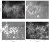 |
Fig. 1. Overview of the observation in Ca II 8542 Å, Fe I 6302 Å and Ca II K. Top row: from the left Stokes I at Δλ = 85 mÅ and V/I at Δλ = 170 mÅ from line center. Bottom row: from the left Stokes V/I of Fe I 6302 Å at Δλ = 40 mÅ from line center and Stokes I of Ca II K at Δλ = 470 mÅ. The red box indicates the area used in our study. |
3. Data analysis
3.1. Inversions
To estimate the thermodynamic and magnetic properties of the region NOAA 2591, we performed NLTE inversions using the STockholm inversion Code (STiC; de la Cruz Rodríguez et al. 2016, 2019). This latter is a modified version of the radiative-transfer RH code (Uitenbroek 2001) and includes a fast approximation to calculate the effects of partial redistribution (PRD, see Leenaarts et al. 2012). The inversion engine of STiC includes an equation of state extracted from the Spectroscopy Made Easy (SME, Piskunov & Valenti 2017). The radiative transport equation is solved using a cubic Bezier solver (de la Cruz Rodríguez & Piskunov 2013) of the polarized transfer equation.
The spectra in the Ca II spectral lines were calculated in NLTE by assuming statistical equilibrium and plane-parallel geometry. Furthermore, PRD effects were explicitly included in the calculations of the H and K lines. The Fe I lines were synthesized assuming LTE. We chose to perform the inversions in a column-mass scale. In comparison to optical depth, column mass allows the gas pressure scale to be computed directly, without involving the equation of state or background opacities. We show below that this feature is important when using the NN to predict models from observations.
We inverted a training set for a NN. The training set consisted of the full FOV for two non consecutive time-steps of the series, but we only inverted every seventh pixel of the FOV in order to speed up the calculations. Furthermore, in order to efficiently train the NN it is more convenient to have a statistical picture of the FOV, with many pixels spread across the region and many different observed spectra, rather than many pixels in a small area that could all present similar observed spectra.
We initialized the magnetic field vector of the initial input model using the spatially-regularized weak-field approximation proposed in Morosin et al. (2020). The presence of strong velocity gradients as a function of depth can greatly distort the line profile of very strong lines. In our tests, this was one of the main sources of degeneracy in the output models. In order to better sample the parameter space in line-of-sight velocity, we prescribed five initializations of the stratification that were added to the FAL-C model (Fontenla et al. 1993): three with constant values at 0, ±5 km s−1, and two with strong upflowing and downflowing gradients (see Fig. 2). The number of nodes used to run the inversion are the same for all five models. We used ten nodes in temperature, four in vLOS, four in vturb, three in B||, two in B⊥, and one node in the azimuth ϕ. For each pixel, we selected the model that yielded the best χ2 value and then applied a mild horizontal smoothing. The inversions were re-started with an increased number of 11 nodes in temperature and 4 nodes in B∥. Once all cycles were finished, we switched on the NLTE equation of state and re-ran the final cycle, which essentially accounts for the ionization of hydrogen in NLTE and the ionization of the rest of elements is calculated in LTE. The last cycle essentially affects the temperature stratification and the derived electron densities.
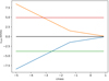 |
Fig. 2. Example of the line-of-sight velocity stratifications as a function of the logarithm of the column mass (ξ), which were used to create the models for the inversions with STiC. |
The first two rows in Fig. 3 present respectively the T and vLOS for three different depths in the atmosphere, which correspond to lower photosphere, upper photosphere, and upper chromosphere. For B||, B⊥, and vturb, just two depths were chosen: these are represented in each column of the two bottom rows.
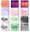 |
Fig. 3. Horizontal cuts from the final model atmosphere obtained from the inversions. The depth in the atmosphere is given in column mass. The T and the vLOS are shown for three different depths, corresponding to lower photosphere, upper photosphere, and chromosphere. B||, B⊥, and vturb are shown for two depths corresponding to lower photosphere and chromosphere. |
The inversion results reproduce many features of the solar atmosphere that are well known from previous research. In the photospheric temperature map, for example, the granulation pattern is visible, while moving upwards in the atmosphere, the hotter and elongated fibrillar structures extend toward the outside. Moreover, the magnetic field presents the typical plage structure with strong concentrations of field and field-free gaps in the photosphere, while in the chromosphere it is more extended and less strong (Buehler et al. 2015; Díaz Baso et al. 2019a; Morosin et al. 2020). We note that the Q and U signals in the chromosphere are very noisy and the inversion code struggles to reconstruct clean maps for the |B⊥| and the azimuthal components of the magnetic field.
Due to the signal-to-noise ratio (S/N) of the observation and the differences in sensitivity of the emerging intensities to the different parameters of the model, the depth resolution of the model is greatest in temperature and line-of-sight velocity, and is much more limited in microturbulence and B∥. Therefore, the magnetic canopy does not appear as sharply in the reconstructed magnetic field stratification as in the temperature reconstruction and in both cases it is much smoother than it probably is in reality because of the limitations of a node-based inversion.
3.2. Neural network application
As it would be extremely time consuming and very computationally expensive to invert all the 35 time-frames of the observation with STiC, we suggest instead an easier and faster approach using NNs. These have shown a good performance in terms of accuracy and speed and have been used to perform a large range of different tasks; for example, to identify and predict solar flares (Panos et al. 2018), to denoise solar observational images (Díaz Baso et al. 2019b), and to learn the mapping between spectral lines and the solar atmosphere (Socas-Navarro 2005; Centeno et al. 2022). In the present case, we used the resulting model atmospheres from the inversion to train a NN that can quickly predict the model atmosphere for the rest of the dataset. We refer the reader to Appendix A for a detailed explanation of the architecture, training process, and validation of the NN.
Results of the NN. The results obtained with the training of the NN are shown in Fig. 4 in a format similar to that of Fig. 3. The represented time-step is the same as in Fig. 3.
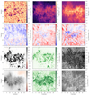 |
Fig. 4. Final model atmosphere of the FOV obtained from the training of the NN. Format as for Fig. 3. |
The temperature and line-of-sight velocity prediction from the NN are very well correlated with the results from the inversions (see 2D density plots in Fig. 5). Both components of the magnetic field vector are predicted to be smoother compared to those obtained with the inversions. The latter occurs because the noise from Stokes Q and U was dominating the inversion results and STiC was not able to fully reconstruct the signal. The introduction of an additional random noise component in the training helps the NN to better generalize the mapping and to obtain a more robust estimation of the values.
 |
Fig. 5. Density plots comparing the results of the inversion with the results of the NN. From the left panels: correlations for T, vLOS, B||, B⊥ and vturb at cmass = −3.1. |
The NN seems to overestimate vturb very deep in the photosphere, while in the chromosphere this behavior disappears. The NN incorrectly correlates areas of strong photospheric B|| with higher values of the microturbulence. We investigated ways of removing this degeneracy, but we could not find a solution. We decided to move forward regardless because the values of the microturbulence close to the continuum formation layer in the photosphere have no influence on the prediction of radiative losses through strong chromospheric lines.
4. Radiative cooling rates
The heating terms in the chromosphere can be approximately estimated by calculating the integrated radiative losses, because the energy required to sustain radiative losses must be sustained by chromospheric heating terms. To calculate the radiative cooling rates from the predicted model atmosphere from the NN, we first imposed hydrostatic equilibrium in order to derive a z-scale and the gas-pressure scale. Most inversion codes operate in an optical-depth scale and therefore the gas pressure has to be calculated iteratively with the consequent re-calculation of the continuum opacity (see, e.g., Mihalas 1970). However, working in a column mass scale simplifies the calculations and no iterations are needed (Hubeny & Mihalas 2014):
 (1)
(1)
where ξ is the column mass, known from the inversions, g⊙ is the solar gravity and pgas is the gas pressure.
We calculated the electron densities in each depth point using a simple equation of state1 proposed by Mihalas (1970) which includes hydrogen atoms bound in H− and H2 molecules. Once the electron densities were known, we estimated the total number of atoms for a given temperature assuming an ideal gas:
 (2)
(2)
where Na is the atoms number density, Ne is the electron density, KB is the Boltzmann constant, and T the temperature. In this way, it is possible to obtain the total number of atoms Na and, by multiplying this by the mean particle mass, we can obtain the density ρ at a certain depth in the atmosphere:
 (3)
(3)
where the mean particle mass ⟨m⟩ is given by:
 (4)
(4)
In this case, ai is the solar abundance of the ith element and mi is its atomic mass.
Finally, we obtained the z-scale from the definition of column mass:
 (5)
(5)
Therefore, in a discrete grid, we can write:
 (6)
(6)
This hydrostatic z-scale is used to calculate the integrated radiative losses in the chromosphere. The latter are calculated integrating over a height interval selected from the z-scale. Our final model contains all the quantities calculated under the assumption of hydrostatic equilibrium and the ones previously obtained after the inversion process.
We used a modified version of STiC that directly evaluates Eq. (7) and also outputs the net radiative rates for all transitions and the atom population densities. In our case, we considered Lyα, Ly continuum, Hα, the Ca II H and K and the IR triplet lines, and the Mg IIh and k and the UV triplet lines. Our inversion setup includes lines that sample the solar atmosphere from the upper chromosphere to the photosphere. Although the Ca II K line may be sensitive to the very lower part of the transition region, it is not sufficient to properly constrain its exact location and gradient. Therefore, the reconstructed transition region is very cold and extended in comparison to models from inversions including transition region diagnostics (see e.g., de la Cruz Rodríguez et al. 2016). The latter seem to have a large impact on the prediction of the Balmer continuum, which is unrealistically large in our calculations. We could not find an obvious solution to this problem, and therefore we did not include the Balmer continuum contribution in our study. The effect of this exclusion is that our radiative losses will potentially be even lower than the heating terms that we are approximating with them.
The inversions were calculated including the effect of NLTE hydrogen ionization in statistical equilibrium by imposing charge conservation (Leenaarts et al. 2007). Our NN does not predict the electron density because the latter is not a parameter of the inversion and STiC can calculate it as a post-processing step. In that way, the electron density is fully consistent with the model atmosphere obtained with the NN and we avoid another potential source of error compared to a computation through the NN. Therefore, we first calculated a forward synthesis with the H atom, recovering not only the radiative losses but also the electron densities in NLTE. We then replaced the electron densities in the original model with the new ones in the input model. The synthesis was done for the Ca II and Mg II atoms with the updated electron densities.
The radiative cooling rates are calculated automatically inside the code by computing the divergence of the radiative flux (see e.g., Uitenbroek 2002; Rutten 2003):
![Mathematical equation: $$ \begin{aligned} Q = \nabla \cdot F = \int _{0}^{\infty } \alpha _{\nu }(z) \left[{S\!}_{\nu }(z) - J_{\nu }(z)\right] \, \mathrm{d} \nu , \end{aligned} $$](/articles/aa/full_html/2022/08/aa43461-22/aa43461-22-eq8.gif) (7)
(7)
where αν is the total absorption coefficient, Sν is the total source function, and Jν is the mean intensity over solid angle. For bound-bound transitions, Eq. (7) can be transformed into an expression that only depends on the net radiative rates and the level population densities:
 (8)
(8)
where h is the Planck’s constant, ν0 is the central frequency of the transition, nu/l are the population of the upper and lower level, respectively, and Rul/lu are the radiative rate coefficient from the upper to the lower level or vice versa.
In order to obtain the integrated radiative losses, Q has to be integrated over the range of geometrical heights of the region of interest. In our case, the integration limits are set in order to take into account only the chromosphere, that is, from the depth point after the temperature minimum to the depth point at which the temperature reaches T ∼ 10 000 K. We note that moving the integration limits can change the derived losses, and therefore some deviations can be expected when comparing numbers from different studies.
5. Results
5.1. Single time-step
In order to study the spatial distribution of radiative losses, we calculated the radiative losses for the initial time-step of the observations. We chose this frame because it is one of those with better seeing conditions. We divided our integration interval (in height) into three subregions (lower, middle, and upper chromosphere) to understand how the energy deposition is taking place; these are shown in Fig. 6. The lower extreme of the interval was chosen after the temperature minimum, that defines the end of the photosphere and the beginning of the chromosphere. The upper extreme was chosen in order not to include the transition region in the calculations. As our inversions did not include lines that are strongly sensitive to the transition region, the steep temperature gradient and its exact location are not well constrained in our models.
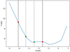 |
Fig. 6. Average temperature for the plage region as a function of cmass. The red dots and the dashed lines represent the total integration interval for the radiative losses, while the green dots and the dotted lines show the division between lower, middle, and upper integration intervals used in Figs. 7 and 8. |
The derived radiative losses integrated over the entire interval and over the three subregions of the chromosphere are shown in the top row of Fig. 7. The average integrated radiative losses over the whole plage region are ∼ − 28 kW m−2. The FOV shows very small-scale regions with peak values of ∼ − 90 kW m−2. In order to obtain greater insight into the calculated radiative losses, we plot in Fig. 8 the contributions of each atom in the three sub-layers of the chromosphere. The Ca II contribution dominates in the lower and middle chromosphere while the contributions from H I and Mg II lines are negligible in this region. The middle chromosphere is the sub-layer that presents the lowest values associated with the radiative losses. In the upper chromosphere, hydrogen is the main contributor to the radiative losses. The contribution from the Mg II atom is approximately one half of that from hydrogen.
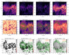 |
Fig. 7. Maps of the radiative losses, temperature, and parallel magnetic field for different heights in the solar atmosphere. Top row: derived radiative losses for the entire FOV for the first time-step. The first panel from the left represents the total radiative losses integrated over the chromosphere. The other three panels show the radiative losses integrated over the lower, middle, and upper chromosphere, respectively. Middle row: maps of the temperature for four different heights in the solar atmosphere. The height increases from left to right. Bottom row: maps of the parallel magnetic field for four different heights in the solar atmosphere. The height is increasing from left to right. The first panels in the middle and bottom rows represent the T and B|| in the photosphere, respectively. The green contours indicate the area where |


The comparison of the integrated radiative losses with the line-of-sight component of the magnetic field provides significant insight into the overall heating process (see Fig. 7). From left to right, the contours plotted in three of the four panels correspond to a fraction of the median value of the radiative losses ( kW m−2, where
  is the average net radiative loss in that layer) in the lower chromosphere, in the middle chromosphere, and in the upper chromosphere. In the lower and middle chromosphere, the bulk of the radiative losses is concentrated in the areas surrounding the strongest photospheric magnetic field concentrations but not inside the latter. The distribution of the largest temperatures is also greatly correlated with the magnetic canopy. The photospheric temperature panel shows that our FOV contains a number of small pores. We discuss the effect of pores in Sect. 5.2. In the lower chromosphere, the peak values of the radiative losses reach ∼ − 20 kW m−2. The lower-left panel in Fig. 8 shows that the Ca II contribution dominates in the lower chromosphere, and the canopy shape is already visible there.
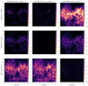 |
Fig. 8. Maps of the contributions to the obtained radiative losses in the lower, middle, and upper layers in the chromosphere per atom. Top row: integrated radiative losses for hydrogen. Middle row: integrated radiative losses for magnesium. Bottom row: integrated radiative losses for calcium. |
In the middle chromosphere, the magnetic field becomes smoother and the magnetic canopy is clearly visible in the B∥ image, suggesting that at this depth we are already sampling above the lower edge of the canopy. The Qmiddle shows a similar picture with slightly smaller radiative losses. The temperature image shows a nearly homogeneous value of approximately 6.5 kK, while most pores appear as cold holes in the canopy.
In the upper chromosphere, the integrated radiative losses are dominated by the H I contribution. In this layer, the radiative losses, the enhanced chromospheric temperature and the magnetic field form a patch above the plage target with relatively constant values of ⟨Q⟩≈ − 22 kW m−2, ⟨T⟩≈8.5 kK and ⟨|B∥|⟩ ≈ 370 G. In this layer only the strongest pores are visible in the temperature map and in the radiative losses map.
5.2. The effect of pores
The presence of pores in plage seem to have a clear imprint in the statistics of the derived physical parameters (see e.g., Chintzoglou et al. 2021). Our target contains several pores, which appear as colder and larger footpoints of the magnetic canopy than in the rest of the magnetic elements. Otherwise, the magnetic field is still strongly vertical. The imprint of pores is clear. Because they are much colder than the smaller bright flux tubes, the radiative losses are insignificant in comparison with the surroundings, until we reach the upper chromosphere. Figure 9 shows a vertical reconstruction, marked with the white slit in Fig. 7. This slice cuts through two pores embedded in the plage region (at Y ∼ 8 arcsec and 8 < X < 22 arcsec), illustrating this effect. The figure also suggests that eventually, the imprint of pores is much smoother and weaker in the upper chromosphere.
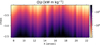 |
Fig. 9. Vertical cut corresponding to the white dashed line of Fig. 7. The total integrated radiative losses have been divided by the model densities ρ and are represented using a symmetrical logarithmic scale. |
In summary, having pores in the FOV does affect the derived radiative losses, especially in the lower chromosphere, because the atmosphere is much colder than in regular flux tubes. In addition, having spatially resolved maps greatly helps to separate their influence from the rest of the FOV.
5.3. Time-series analysis
The NN makes it possible to obtain the model atmosphere for all the time-steps of the observation, and therefore allows us to estimate a time-series of integrated radiative losses in the chromosphere over the entire FOV. We focus on the red region highlighted in the top left panel of Fig. 7 and we calculated the radiative energy balance for 21 time-steps of the whole observations. Given the cadence of the CRISP instrument, the latter cover a total time of Δt = 12.19 min. In Sect. 1 we mention that magnetoacoustic waves and shocks can contribute significantly to the heating of plage, and their imprint should be periodic. Our aim is to separate the contribution of Ohmic heating from the contribution of waves and shocks (De Pontieu et al. 2007; Hasan & van Ballegooijen 2008) by analyzing a time-series.
In order to get an idea of the dominant period (p), amplitude (A), phase (ϕ) and offset (Coff) of the oscillatory behavior, we fitted a very simple model y = Coff + A ⋅ sin(ϕ + pt) to the vLOS and Qtot temporal curves. The results for two random pixels are shown in the left and in the middle panels of Fig. 10. The selected pixels are marked with green crosses in Fig. 7. The vLOS is estimated in the region at cmass = −3.8, corresponding to middle and upper chromosphere. The results are in line with previous studies about wave propagation in different targets of the solar atmosphere. Both curves have very similar periods, but there is a phase shift between Qtot and vLOS, which we discuss below.
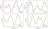 |
Fig. 10. Time-evolution of the radiative losses and of vLOS for two selected pixels and a region in the FOV. The two chosen pixels are indicated with green crosses in Fig. 7. Left: time-evolution of Q (top panel) and vLOS (bottom panel) for the first random pixel. Right: time-evolution of Q (top panel) and vLOS (bottom panel) for the second random pixel. |
The fitting procedure has been extended to the red highlighted region in the left top panel of Fig. 7. We plotted a map for each parameter of the sinusoidal function in Fig. 11. The displayed parameters represent the quantities characterizing the time-evolution of Q, vLOS and vturb (from the top row). As a reference, average values of the parameters over the region are given in Table 2. In our model, the offset is the value of Q or vLOS not related to the periodic wave. In the case of the radiative losses, our interpretation is that it contains the contribution from other heating phenomena, such as Ohmic dissipation, ion-neutral collisions, and so on. The top-left panel of Fig. 11 shows a smooth distribution of the offset values. Although the smallest scales are not present in this plot, there is large-scale variation across the panel.
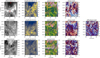 |
Fig. 11. Maps of the parameters (offset, amplitude, period, and phase) of the sinusoidal functions obtained for the red region of Fig. 7. Top row: quantities characterizing the sinusoidal time-evolution of the radiative losses, while the second row represents the quantities characterizing the time-evolution of vLOS at cmass = −3.8. In the maps of the period, yellow contours indicate the plage area corresponding to Q < −20 kW m−2 (see Fig. 7). The first column from the right shows the phase difference between Q and vLOS. Bottom row: quantities of the sinusoidal evolution for vturb at cmass = −3.8. |
If we neglect the upper central part of the maps, outside the boundary of the plage region, the average amplitudes become  kW m−2 and
  km s−1. The latter is in agreement with values reported by Centeno et al. (2009) in a facular region using the He I 10830 Å line. The relatively large value of the period in the chromosphere could be due to the propagation along an inclined magnetic field line which can extend the cut-off frequency in the chromosphere (e.g., Bloomfield et al. 2007).
The third column of Fig. 11 shows the period maps of both Q an vLOS. The yellow contours indicate those areas where the radiative losses are particularly strong (Q < −20 kW m−2). The average period of oscillation for Q is  min, while considering only the region inside the contour it drops to
  min. These results found for vLOS are in line with previous works (de Pontieu 2004; Centeno et al. 2009), with a value of
  min. We note that in the plage area (bottom half of the panel) the periods present a relatively smooth distribution, between 4 and 5 min, whereas the upper area of the image, outside the plage region, shows elongated features with longer periods. The latter is located at the plage boundary, where the magnetic field is more horizontal. The phase difference between the radiative losses and the line-of-sight velocity is dominated by values close to π/2. As the behavior of the radiative losses is dominated by the temperature, we are recovering the usual phase relation for running waves.
Although we do not include plots showing the imprint of the periodic signal in each of the sub-layers of the chromosphere investigated here, we performed the fits individually for each layer. In the lower and middle chromosphere, the modulation amplitude is of the order of 1 kW m−2, whereas in the upper chromosphere we get values much closer to the integral over the entire chromosphere. Therefore, we can conclude that although the imprint of waves is present in the lower and middle chromosphere, their contribution is larger in the upper chromosphere.
A potential source of error in our results is the presence of stray light in the data. The effect of stray light in the intensity images is to decrease the rms contrast of small-scale features. We estimate the Strehl ratio of our observations to be 0.6. According to Scharmer et al. (2019), for that Strehl ratio, the main stray-light contribution at the SST and its instrumentation is from uncorrected high-order aberrations, with a dominant contribution from within 1″ radius (see also, Scharmer et al. 2011). However, we cannot directly translate the effect of stray light into a quantitative estimate of the error in the derived radiative losses. The offset map shows blobs with typical sizes of 1 − 2″ and therefore we estimate the effect of stray light to be minimal there. Nevertheless, the amplitude of the periodic component map shows fine structure down to 0.2″, which is significantly smaller than the expected stray-light PSF radius. Although it is clear that stray light is not washing out the smallest scales, they must still be affected by it. Therefore, we conclude that the amplitudes of the periodic component, which we associate with wave heating, are more affected by stray light than the offset map. The estimated contribution of wave heating to the net radiative losses must therefore be considered a lower limit.
6. Discussion and conclusions
Our temporal analysis allows us to quantify the contribution from a periodic component, which we associate with wave heating. This component is weaker than the offset (background) value of the heating terms and has a mean modulation amplitude of ∼7.0 kW m−2. This component is responsible for the very fine structure that we observe in the Qtot maps. The offset value, which we associate with a more static or very slowly evolving component, has a mean value of ∼ − 26.1 kW m−2. The map constructed from the offset value is relatively smooth, which could also point to a magnetic origin. On the Sun, the β = 2μPg/B2 = 1 layer is usually located in the lower chromosphere, and therefore the magnetic field becomes smooth and room-filling above that layer. Having a relatively smooth offset map signals a magnetic origin. The amplitude of the periodic component of the radiative losses is almost a factor four larger in the upper chromosphere than in the lower and middle regions. Given the spatial distribution of periods and the relatively homogeneous π/2 phase difference, we associate the periodic component with compressible acoustic waves (the slow-mode of magnetoacoustic waves when vA > cs). This argument is further supported by Fig. 12, where we show the time-evolution of the 8542 Å line at three random pixels selected in the middle of the canopy areas that are located in the surroundings of the photospheric magnetic elements. In all cases, the classical saw-tooth pattern from acoustic shocks is clearly visible (see, e.g., Carlsson & Stein 1992; Langangen et al. 2008; Vecchio et al. 2009).
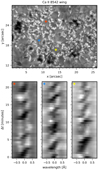 |
Fig. 12. Overview of the FOV in Ca II 8542 Å and time-evolution of the 8542 Å line at three random pixels. Lower row: time-evolution of the Ca II 8542 Å line at three locations, picked in the middle of the canopy regions, which are surrounded by the photospheric magnetic elements. The locations of the three pixels are marked in the upper panel with colored cross-like markers. |
Our results show that in the lower and middle chromosphere the radiative losses are distributed in areas surrounding the photospheric footpoints of the magnetic canopy. We do not see enhanced radiative losses within the magnetic footpoints of the canopy. Furthermore, de la Cruz Rodríguez et al. (2013) showed that in those canopy regions the Ca II 8542 Å line profiles have a peculiar shape that can be explained by the presence of a hot magnetic canopy in the chromosphere that extends over a relatively quiet photosphere. The magnetic canopy should have a relatively sharp lower edge, where current sheets should be found through the relation j = ∇ × B/μ. Although, our inverted models have a low depth resolution in the magnetic field reconstruction due to the S/N of our observations, the temperature stratification was derived with more than twice the number of nodes and we do see a relatively sharp canopy boundary there. Therefore, we argue that in the lower chromosphere of plage, Ohmic current dissipation must be responsible for the bulk of the heating. We also argue that if wave heating were a dominant phenomena in the lower chromosphere, its imprint should also be visible inside the magnetic footpoints, which we do not observe in our results (see e.g., Hasan & van Ballegooijen 2008). Brandenburg & Rempel (2019) also showed that Ohmic dissipation works efficiently in the photosphere and the lower chromosphere.
In the upper chromosphere, the radiative losses form a patch that covers the entire plage region, including most of the pores that are present in the photosphere. Within this patch, the derived chromospheric temperatures are relatively homogeneous and larger than in the surroundings, with temperatures the order of ∼7.5 − 8 kK and a magnetic field strength of the order of ∼400 G. The largest contribution to the integrated radiative losses is from the H I diagnostics in the upper chromosphere. The contribution of wave heating is, in our results, largest in this layer. From our results alone, we cannot claim to have direct evidence of turbulent Alfvén wave heating (van Ballegooijen et al. 2011) or from neutral-ion collisions (Khomenko & Collados 2012). Given the smooth nature of the magnetic field, we do not expect current sheets to be present in the upper chromosphere, making Ohmic dissipation of currents a less likely heating mechanism. The periodic behavior that we observe has a relatively long period of 5.5 min. At a cadence of ∼30 s, wave patterns with periods lower than 1 min are not properly sampled in our observations, and so we cannot resolve high-frequency waves.
In order to further investigate the origin of the wave behavior and the deposition of energy in the chromosphere, we briefly extended our study to the microturbulence velocity vturb. However, the temporal analysis, represented in the last row of Fig. 11, does not show a clear pattern in the offset or in the amplitude. This pattern is definitely different from the typical white noise, but does not correlate with the patterns shown in the panels of Q or vLOS. We might expect an imprint of the wave pattern in the microturbulence if the shocks were relatively unresolved in depth by the inversion code, forcing a larger microturbulence value to account for the extra broadening. We do not observe such behavior.
Our results are somewhat different from those reported by Anan et al. (2021), but are surprisingly compatible. Their observations were based on arguably lower spatial-resolution slit-spectrograph raster scans in the Mg IIh and k lines (IRIS) and in the He I 10830 Å line. Although the analysis of these latter authors was not based on the calculation of radiative losses, they used the integrated h and k line intensity as a proxy, in a similar way to Leenaarts et al. (2018), who used the Ca IIh and k lines. We have shown that the radiative losses in the lower chromosphere are very small in the Mg II lines. By not having the Ca II deeper contribution, Anan et al. (2021) would also miss the heating closer to the lower boundary of the magnetic canopy. As for the estimates of the chromospheric magnetic field made by these latter authors, they are based on inversions of the He I 10830 Å line, and the latter usually samples the middle and upper chromosphere (see Fig. 1 in de la Cruz Rodríguez et al. 2019) according to estimates from numerical simulations.
The present study is unique in that we calculated and studied the distribution of radiative losses as a function of depth and time from very high-spatial-resolution spectra. The canonical value of QAR ∼ 20 kW m−2 derived in the 1970s and 1980s using spatially and temporally averaged spectra is unlikely to capture the complexity and dynamic behavior of the solar chromosphere as shown in our analysis. Our analysis is also different from previous studies in that we estimated the contribution from waves directly from the periodic modulation of the radiative losses, and not by estimating the energy that is carried out by waves in the chromosphere from Doppler velocities (Abbasvand et al. 2020).
Ultimately, our results do not provide direct evidence allowing us to decipher the dominant heating mechanism in the upper chromosphere. In our opinion, future studies of the same nature should analyze higher cadence time-series and higher spatial-resolution observations in order to search for observational signatures of high-frequency waves or very small-spatial-scale variations that could point to turbulent Alfvén wave dissipation. In order to estimate ambipolar diffusion heating, an accurate estimate of the upper chromosphere density is also needed, and therefore inversion codes must be modified in order to include the Lorentz force (Pastor Yabar et al. 2019, 2021) and the support effects derived from velocity gradients.
Acknowledgments
This project has received funding from the European Research Council (ERC) under the European Union’s Horizon 2020 research and innovation program (SUNMAG, grant agreement 759548). J.L. is supported through the CHROMATIC project (2016.0019) funded by the Knut och Alice Wallenberg foundation. The Swedish 1-m Solar Telescope is operated on the island of La Palma by the Institute for Solar Physics of Stockholm University in the Spanish Observatorio del Roque de los Muchachos of the Instituto de Astrofísica de Canarias. The Institute for Solar Physics is supported by a grant for research infrastructures of national importance from the Swedish Research Council (registration number 2017-00625). This research has made use of NASA’s Astrophysics Data System Bibliographic Services. The computations were enabled by resources provided by the Swedish National Infrastructure for Computing (SNIC) at the PDC Center for High Performance Computing, KTH Royal Institute of Technology, partially funded by the Swedish Research Council through grant agreement no. 2021/1-12.
References
- Abbasvand, V., Sobotka, M., Švanda, M., et al. 2020, A&A, 642, A52 [EDP Sciences] [Google Scholar]
- Anan, T., Schad, T. A., Kitai, R., et al. 2021, ApJ, 921, 39 [NASA ADS] [CrossRef] [Google Scholar]
- Asensio Ramos, A., & Díaz Baso, C. J. 2019, A&A, 626, A102 [NASA ADS] [CrossRef] [EDP Sciences] [Google Scholar]
- Asensio Ramos, A., Trujillo Bueno, J., & Landi Degl’Innocenti, E. 2008, ApJ, 683, 542 [Google Scholar]
- Bishop, C. M. 1995, Neural Networks for Pattern Recognition (USA: Oxford University Press, Inc.) [Google Scholar]
- Bloomfield, D. S., Lagg, A., & Solanki, S. K. 2007, ApJ, 671, 1005 [NASA ADS] [CrossRef] [Google Scholar]
- Brandenburg, A., & Rempel, M. 2019, ApJ, 879, 57 [NASA ADS] [CrossRef] [Google Scholar]
- Buehler, D., Lagg, A., Solanki, S. K., & van Noort, M. 2015, A&A, 576, A27 [NASA ADS] [CrossRef] [EDP Sciences] [Google Scholar]
- Carlsson, M., & Stein, R. F. 1992, ApJ, 397, L59 [Google Scholar]
- Carlsson, M., Leenaarts, J., & De Pontieu, B. 2015, ApJ, 809, L30 [NASA ADS] [CrossRef] [Google Scholar]
- Carlsson, M., De Pontieu, B., & Hansteen, V. H. 2019, ARA&A, 57, 189 [Google Scholar]
- Centeno, R., Collados, M., & Trujillo Bueno, J. 2009, ApJ, 692, 1211 [Google Scholar]
- Centeno, R., Flyer, N., Mukherjee, L., et al. 2022, ApJ, 925, 176 [NASA ADS] [CrossRef] [Google Scholar]
- Chintzoglou, G., De Pontieu, B., Martínez-Sykora, J., et al. 2021, ApJ, 906, 83 [NASA ADS] [CrossRef] [Google Scholar]
- da Silva Santos, J. M., de la Cruz Rodríguez, J., Leenaarts, J., et al. 2020, A&A, 634, A56 [NASA ADS] [CrossRef] [EDP Sciences] [Google Scholar]
- da Silva Santos, J. M., Danilovic, S., Leenaarts, J., et al. 2022, A&A, 661, A59 [NASA ADS] [CrossRef] [EDP Sciences] [Google Scholar]
- de la Cruz Rodríguez, J., & Piskunov, N. 2013, ApJ, 764, 33 [Google Scholar]
- de la Cruz Rodríguez, J., De Pontieu, B., Carlsson, M., & Rouppe van der Voort, L. H. M. 2013, ApJ, 764, L11 [CrossRef] [Google Scholar]
- de la Cruz Rodríguez, J., Löfdahl, M. G., Sütterlin, P., Hillberg, T., & Rouppe van der Voort, L. 2015, A&A, 573, A40 [NASA ADS] [CrossRef] [EDP Sciences] [Google Scholar]
- de la Cruz Rodríguez, J., Leenaarts, J., & Asensio Ramos, A. 2016, ApJ, 830, L30 [Google Scholar]
- de la Cruz Rodríguez, J., Leenaarts, J., Danilovic, S., & Uitenbroek, H. 2019, A&A, 623, A74 [Google Scholar]
- de Pontieu, B. 2004, in SOHO 13 Waves, Oscillations and Small-Scale Transients Events in the Solar Atmosphere: Joint View from SOHO and TRACE, ed. H. Lacoste, ESA Spec. Publ., 547, 25 [NASA ADS] [Google Scholar]
- De Pontieu, B., Hansteen, V. H., Rouppe van der Voort, L., van Noort, M., & Carlsson, M. 2007, ApJ, 655, 624 [Google Scholar]
- De Pontieu, B., McIntosh, S., Martinez-Sykora, J., Peter, H., & Pereira, T. M. D. 2015, ApJ, 799, L12 [Google Scholar]
- Díaz Baso, C. J., Martínez González, M. J., Asensio Ramos, A., & de la Cruz Rodríguez, J. 2019a, A&A, 623, A178 [NASA ADS] [CrossRef] [EDP Sciences] [Google Scholar]
- Díaz Baso, C. J., de la Cruz Rodríguez, J., & Danilovic, S. 2019b, A&A, 629, A99 [NASA ADS] [CrossRef] [EDP Sciences] [Google Scholar]
- Díaz Baso, C. J., de la Cruz Rodríguez, J., & Leenaarts, J. 2021a, A&A, 647, A188 [NASA ADS] [CrossRef] [EDP Sciences] [Google Scholar]
- Díaz Baso, C., Vissers, G., Calvo, F., et al. 2021b, https://doi.org/10.5281/zenodo.5608441 [Google Scholar]
- Díaz Baso, C. J., Asensio Ramos, A., & de la Cruz Rodríguez, J. 2022, A&A, 659, A165 [NASA ADS] [CrossRef] [EDP Sciences] [Google Scholar]
- Fontenla, J. M., Avrett, E. H., & Loeser, R. 1993, ApJ, 406, 319 [Google Scholar]
- Hasan, S. S., & van Ballegooijen, A. A. 2008, ApJ, 680, 1542 [NASA ADS] [CrossRef] [Google Scholar]
- Hubeny, I., & Mihalas, D. 2014, Theory of Stellar Atmospheres (Princeton: Princeton University Press) [Google Scholar]
- Ishikawa, R., Bueno, J. T., del Pino Alemán, T., et al. 2021, Sci. Adv., 7, eabe8406 [NASA ADS] [CrossRef] [Google Scholar]
- Khomenko, E., & Collados, M. 2012, ApJ, 747, 87 [Google Scholar]
- Kianfar, S., Leenaarts, J., Danilovic, S., de la Cruz Rodríguez, J., & Díaz Baso, C. J. 2020, A&A, 637, A1 [NASA ADS] [CrossRef] [EDP Sciences] [Google Scholar]
- Kingma, D. P., & Ba, J. 2017, ArXiv e-prints [arXiv:1412.6980] [Google Scholar]
- Koenker, R. W., & Bassett, G. 1978, Econometrica, 46, 33 [CrossRef] [Google Scholar]
- Langangen, Ø., Carlsson, M., Rouppe van der Voort, L., Hansteen, V., & De Pontieu, B. 2008, ApJ, 673, 1194 [NASA ADS] [CrossRef] [Google Scholar]
- Leenaarts, J., Carlsson, M., Hansteen, V., & Rutten, R. J. 2007, A&A, 473, 625 [NASA ADS] [CrossRef] [EDP Sciences] [Google Scholar]
- Leenaarts, J., Pereira, T., & Uitenbroek, H. 2012, A&A, 543, A109 [NASA ADS] [CrossRef] [EDP Sciences] [Google Scholar]
- Leenaarts, J., de la Cruz Rodríguez, J., Danilovic, S., Scharmer, G., & Carlsson, M. 2018, A&A, 612, A28 [NASA ADS] [CrossRef] [EDP Sciences] [Google Scholar]
- Löfdahl, M. G., Hillberg, T., de la Cruz Rodríguez, J., et al. 2021, A&A, 653, A68 [Google Scholar]
- Martínez-Sykora, J., De Pontieu, B., Hansteen, V. H., et al. 2017, Science, 356, 1269 [Google Scholar]
- Mihalas, D. 1970, Stellar Atmospheres (San Francisco: Freeman) [Google Scholar]
- Milić, I., & van Noort, M. 2018, A&A, 617, A24 [Google Scholar]
- Morosin, R., de la Cruz Rodríguez, J., Vissers, G. J. M., & Yadav, R. 2020, A&A, 642, A210 [NASA ADS] [CrossRef] [EDP Sciences] [Google Scholar]
- Nair, V., & Hinton, G. E. 2010, Rectified Linear Units Improve Restricted Boltzmann Machines, ICML, 807 [Google Scholar]
- Panos, B., Kleint, L., Huwyler, C., et al. 2018, ApJ, 861, 62 [Google Scholar]
- Pastor Yabar, A., Borrero, J. M., & Ruiz Cobo, B. 2019, A&A, 629, A24 [NASA ADS] [CrossRef] [EDP Sciences] [Google Scholar]
- Pastor Yabar, A., Borrero, J. M., Quintero Noda, C., & Ruiz Cobo, B. 2021, A&A, 656, L20 [NASA ADS] [CrossRef] [EDP Sciences] [Google Scholar]
- Pietrow, A. G. M., Kiselman, D., de la Cruz Rodríguez, J., et al. 2020, A&A, 644, A43 [NASA ADS] [CrossRef] [EDP Sciences] [Google Scholar]
- Piskunov, N., & Valenti, J. A. 2017, A&A, 597, A16 [NASA ADS] [CrossRef] [EDP Sciences] [Google Scholar]
- Priest, E. 2014, Magnetohydrodynamics of the Sun (Cambridge: Cambridge University Press) [Google Scholar]
- Priest, E. R., Chitta, L. P., & Syntelis, P. 2018, ApJ, 862, L24 [Google Scholar]
- Ripley, B. D. 1996, Pattern Recognition and Neural Networks (Cambridge: Cambridge University Press) [CrossRef] [Google Scholar]
- Ruiz Cobo, B., Quintero Noda, C., Gafeira, R., et al. 2022, A&A, 660, A37 [NASA ADS] [CrossRef] [EDP Sciences] [Google Scholar]
- Rutten, R. J. 2003, Radiative Transfer in Stellar Atmospheres, 255 [Google Scholar]
- Sanchez Almeida, J., & Martinez Pillet, V. 1994, ApJ, 424, 1014 [NASA ADS] [CrossRef] [Google Scholar]
- Scharmer, G. 2017, SOLARNET IV: The Physics of the Sun from the Interior to the Outer Atmosphere, 85 [Google Scholar]
- Scharmer, G. B., Bjelksjo, K., Korhonen, T. K., Lindberg, B., & Petterson, B. 2003, in The 1-meter Swedish Solar Telescope, eds. S. L. Keil, & S. V. Avakyan, SPIE Conf. Ser., 4853, 341 [NASA ADS] [Google Scholar]
- Scharmer, G. B., Narayan, G., Hillberg, T., et al. 2008, ApJ, 689, L69 [Google Scholar]
- Scharmer, G. B., Henriques, V. M. J., Kiselman, D., & de la Cruz Rodríguez, J. 2011, Science, 333, 316 [Google Scholar]
- Scharmer, G. B., Löfdahl, M. G., Sliepen, G., & de la Cruz Rodríguez, J. 2019, A&A, 626, A55 [NASA ADS] [CrossRef] [EDP Sciences] [Google Scholar]
- Schmidhuber, J. 2015, Neural Netw., 61, 85 [CrossRef] [Google Scholar]
- Shine, R. A., & Linsky, J. L. 1974, Sol. Phys., 39, 49 [NASA ADS] [CrossRef] [Google Scholar]
- Socas-Navarro, H. 2005, ApJ, 621, 545 [Google Scholar]
- Socas-Navarro, H., de la Cruz Rodríguez, J., Asensio Ramos, A., Trujillo Bueno, J., & Ruiz Cobo, B. 2015, A&A, 577, A7 [NASA ADS] [CrossRef] [EDP Sciences] [Google Scholar]
- Uitenbroek, H. 2001, ApJ, 557, 389 [Google Scholar]
- Uitenbroek, H. 2002, ApJ, 565, 1312 [NASA ADS] [CrossRef] [Google Scholar]
- van Ballegooijen, A. A., Asgari-Targhi, M., Cranmer, S. R., & DeLuca, E. E. 2011, ApJ, 736, 3 [Google Scholar]
- van Noort, M., Rouppe van der Voort, L., & Löfdahl, M. G. 2005, Sol. Phys., 228, 191 [Google Scholar]
- Vecchio, A., Cauzzi, G., & Reardon, K. P. 2009, A&A, 494, 269 [NASA ADS] [CrossRef] [EDP Sciences] [Google Scholar]
- Vernazza, J. E., Avrett, E. H., & Loeser, R. 1981, ApJS, 45, 635 [Google Scholar]
- Withbroe, G. L., & Noyes, R. W. 1977, ARA&A, 15, 363 [Google Scholar]
- Yadav, N., Cameron, R. H., & Solanki, S. K. 2020, ApJ, 894, L17 [Google Scholar]
Appendix A: Training of the neural network
In general, an artificial neural network (ANN) is defined by the dimensionality of the input, the number of layers, the number of neurons per layer, and the dimensionality of the output. The number of neurons in each layer does not have to be constant, and can vary depending on the complexity of the problem. The most commonly used type of NN is the fully connected network (FCN; Schmidhuber 2015), in which every input is connected to every neuron of the following layer. Figure A.1 shows, in a simplified way, the architecture and connections of a FCN. Each connection is described by a simple function that linearly combines the input x multiplied by a weight w and summed with a bias b and finally returns the value of a certain user-defined nonlinear function f(x). In mathematical notation, the information that will pass from the input neurons i to the neuron j of the next layer will be:
 (A.1)
(A.1)
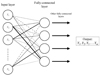 |
Fig. A.1. Simplified representation of a fully connected NN. The lines that connect the inputs with the neurons are represented in different styles (straight, doted, dashed, etc.) because they involve different weights. |
This output will be the input for another neuron of the next layer. As the first operation is linear, the activation is the one that introduces the nonlinear character of the FCNs.
The optimization of a NN is called training and it involves the iterative modification of the weights and biases so that a loss function that measures the ability of the network to predict the output from the input is minimized. In our case, we trained the NN to learn the mapping between the observed Stokes profiles and the model atmosphere obtained from the inversion. Once the network is trained, we are able to reconstruct the temperature T, the line-of-sight velocity vLOS, the turbulence velocity vturb, the parallel component of the magnetic field B||, the perpendicular component |B⊥|, and the azimuth angle ϕ for the entire time-series. The dimensions of the input are defined by the total number of pixels and by the four Stokes parameters. On the other hand, the output dimensions are the total number of pixels and the number of obtained parameters multiplied by the number of grid points.
A.1. Architecture of the NN:
For our purposes, we design a fully connected NN with five layers and 200 neurons per layer. After many tests, we find this configuration to be optimal in terms of training time and accuracy. The activation function that we decided to use is the rectified linear unit or ReLU (Nair & Hinton 2010). It has a linear behavior for a positive input; otherwise, if the input is negative, it is equal to zero:
 (A.2)
(A.2)
It is applied after every layer of the NN, except for the last one, to avoid obtaining only positive outputs.
During the design of the network architecture we detected that the noise in the polarization was amplified and propagated to some physical parameters. To avoid this problem, we decided to split the model into two parts: only Stokes I was employed in the calculation of the temperature and vLOS, while all the four Stokes parameters are used for the other quantities of the model atmosphere. Although Stokes Q, U, and V contain information on the gradient of the source function and the line-of-sight velocity stratification, in cases where the profiles are very noisy they do not play an important role in the derivation of the temperature or line-of-sight velocity, and so it is better to avoid propagating that noise.
A.2. Training process and validation set:
Optimization is routinely solved using simple first-order gradient-descent algorithms, which modify the weights along the negative gradient of the loss function with respect to the model parameters. To scale the magnitude of our weight updates, we have to use the parameter called learning rate. This parameter has to be adjusted to find a compromise between network accuracy and convergence speed. If this number is too small, it will take too long to reach the solution, while if it is too large, there is a risk of overshooting the optimal solution. In our case, we used a learning rate of 10−4. For the optimization method, we used a gradient descent variant called Adam (Kingma & Ba 2017) which was developed to automatically adjust the learning rate, making the solution convergence faster.
Our goal is to optimize a user-defined loss function that evaluates how well our network models the data. The most common loss function is the mean squared error which measures the average squared difference between predictions and desirable outputs. However, to get an idea of the dispersion of the estimate we used the quantile regression (Koenker & Bassett 1978), a loss function for estimating any percentile value:
 (A.3)
(A.3)
where y is the training value and f(x) is output value of the network. During training, q is randomly varied between 0 and 1 so that the network can learn all possible percentiles. This allows us to estimate not only the mean value (q = 0.5) but also the dispersion (q = 0.16 and q = 0.84) which is equivalent to one standard deviation σ in the case of a normal distribution. The dispersion can give us an idea of the uncertainty of the inversion because similar Stokes parameters could have had different atmospheric models as solutions (Díaz Baso et al. 2022).
The gradient of the loss function with respect to the free parameters of the network is obtained using the backpropagation algorithm. As the networks are defined as a stack of layers, the gradient of the loss function can be calculated by the chain rule as the product of the gradient of each module and ultimately of the last layer and the specific loss function. The main problem with some activation functions is that the gradient vanishes for very large values due to the derivative of this function, making it difficult to train the network. For this reason, we used the ReLU function, which does not saturate for large values.
Regarding the dataset, we used two nonconsecutive time-steps of the observations to train the NN in order to include more statistics in our training set, which correspond to about 41160 pixels. To further increase the diversity of profiles used for training the network, we added a Gaussian noise component to the input profiles during the training to make the network prediction more robust to the noise.
Because of the large number of free parameters in a network, overfitting can be a problem. One would like the network to generalize well and avoid any memorization of the training set (Bishop 1995; Ripley 1996). To check that, a part of the dataset is not used during the training but used after each iteration as validation. Desirably, the loss should decrease both in the training and validation sets simultaneously. If overfitting occurs, the loss in the validation set will increase. We randomly chose 90% of the dataset as the training set and the 10% as the validation set. Furthermore, every time that the loss function –calculated with the validation set– reached its minimum, we saved the model parameters. The training was done in a GeForce RTX 2080 Ti GPU for 400000 epochs. Once we had picked the best weights and biases, we were able to apply the obtained model to the other time-step of the observations.
As a final test, we synthesized the spectra from the results of the NN and compared them with the observed profiles and with the synthetic spectra obtained from the inversion process. The results are shown in Fig. A.2. We selected two random pixels and two different time-steps. The four lines (Ca II K, Fe I 6301/6302 Å and Ca II 8542 Å) and the continuum point used for the inversions are represented. The synthetic spectra from the inversion process were only obtained for the two time-steps used in the training process. In the case of the sixth time-step, the comparison was made between the observed spectra and the ones synthesized from the results of the NN. The plots show an overall agreement between the results of the NN and the observed and synthetic profiles.
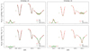 |
Fig. A.2. Comparison between spectra synthesized from the results of the NN (red lines), synthetic spectra from the inversion process (black dashed lines) and observed spectra (green dots) for two different time-steps. The synthetic spectra from the inversions were only calculated for the initial time-step. The two random pixels selected are indicated in the upper left panel of Fig. 11. |
All Tables
Observed line positions of the lines used in this study, relative to line center.
All Figures
|
Fig. 1. Overview of the observation in Ca II 8542 Å, Fe I 6302 Å and Ca II K. Top row: from the left Stokes I at Δλ = 85 mÅ and V/I at Δλ = 170 mÅ from line center. Bottom row: from the left Stokes V/I of Fe I 6302 Å at Δλ = 40 mÅ from line center and Stokes I of Ca II K at Δλ = 470 mÅ. The red box indicates the area used in our study. |
| In the text | |
|
Fig. 2. Example of the line-of-sight velocity stratifications as a function of the logarithm of the column mass (ξ), which were used to create the models for the inversions with STiC. |
| In the text | |
|
Fig. 3. Horizontal cuts from the final model atmosphere obtained from the inversions. The depth in the atmosphere is given in column mass. The T and the vLOS are shown for three different depths, corresponding to lower photosphere, upper photosphere, and chromosphere. B||, B⊥, and vturb are shown for two depths corresponding to lower photosphere and chromosphere. |
| In the text | |
|
Fig. 4. Final model atmosphere of the FOV obtained from the training of the NN. Format as for Fig. 3. |
| In the text | |
|
Fig. 5. Density plots comparing the results of the inversion with the results of the NN. From the left panels: correlations for T, vLOS, B||, B⊥ and vturb at cmass = −3.1. |
| In the text | |
|
Fig. 6. Average temperature for the plage region as a function of cmass. The red dots and the dashed lines represent the total integration interval for the radiative losses, while the green dots and the dotted lines show the division between lower, middle, and upper integration intervals used in Figs. 7 and 8. |
| In the text | |
|
Fig. 7. Maps of the radiative losses, temperature, and parallel magnetic field for different heights in the solar atmosphere. Top row: derived radiative losses for the entire FOV for the first time-step. The first panel from the left represents the total radiative losses integrated over the chromosphere. The other three panels show the radiative losses integrated over the lower, middle, and upper chromosphere, respectively. Middle row: maps of the temperature for four different heights in the solar atmosphere. The height increases from left to right. Bottom row: maps of the parallel magnetic field for four different heights in the solar atmosphere. The height is increasing from left to right. The first panels in the middle and bottom rows represent the T and B|| in the photosphere, respectively. The green contours indicate the area where |
| In the text | |
|
Fig. 8. Maps of the contributions to the obtained radiative losses in the lower, middle, and upper layers in the chromosphere per atom. Top row: integrated radiative losses for hydrogen. Middle row: integrated radiative losses for magnesium. Bottom row: integrated radiative losses for calcium. |
| In the text | |
|
Fig. 9. Vertical cut corresponding to the white dashed line of Fig. 7. The total integrated radiative losses have been divided by the model densities ρ and are represented using a symmetrical logarithmic scale. |
| In the text | |
|
Fig. 10. Time-evolution of the radiative losses and of vLOS for two selected pixels and a region in the FOV. The two chosen pixels are indicated with green crosses in Fig. 7. Left: time-evolution of Q (top panel) and vLOS (bottom panel) for the first random pixel. Right: time-evolution of Q (top panel) and vLOS (bottom panel) for the second random pixel. |
| In the text | |
|
Fig. 11. Maps of the parameters (offset, amplitude, period, and phase) of the sinusoidal functions obtained for the red region of Fig. 7. Top row: quantities characterizing the sinusoidal time-evolution of the radiative losses, while the second row represents the quantities characterizing the time-evolution of vLOS at cmass = −3.8. In the maps of the period, yellow contours indicate the plage area corresponding to Q < −20 kW m−2 (see Fig. 7). The first column from the right shows the phase difference between Q and vLOS. Bottom row: quantities of the sinusoidal evolution for vturb at cmass = −3.8. |
| In the text | |
|
Fig. 12. Overview of the FOV in Ca II 8542 Å and time-evolution of the 8542 Å line at three random pixels. Lower row: time-evolution of the Ca II 8542 Å line at three locations, picked in the middle of the canopy regions, which are surrounded by the photospheric magnetic elements. The locations of the three pixels are marked in the upper panel with colored cross-like markers. |
| In the text | |
|
Fig. A.1. Simplified representation of a fully connected NN. The lines that connect the inputs with the neurons are represented in different styles (straight, doted, dashed, etc.) because they involve different weights. |
| In the text | |
|
Fig. A.2. Comparison between spectra synthesized from the results of the NN (red lines), synthetic spectra from the inversion process (black dashed lines) and observed spectra (green dots) for two different time-steps. The synthetic spectra from the inversions were only calculated for the initial time-step. The two random pixels selected are indicated in the upper left panel of Fig. 11. |
| In the text | |
Current usage metrics show cumulative count of Article Views (full-text article views including HTML views, PDF and ePub downloads, according to the available data) and Abstracts Views on Vision4Press platform.
Data correspond to usage on the plateform after 2015. The current usage metrics is available 48-96 hours after online publication and is updated daily on week days.
Initial download of the metrics may take a while.