| Issue |
A&A
Volume 664, August 2022
|
|
|---|---|---|
| Article Number | A156 | |
| Number of page(s) | 17 | |
| Section | Planets and planetary systems | |
| DOI | https://doi.org/10.1051/0004-6361/202243065 | |
| Published online | 25 August 2022 | |
Uncovering the true periods of the young sub-Neptunes orbiting TOI-2076★
1
Physikalisches Institut, University of Bern,
Gesellsschaftstrasse 6,
3012
Bern, Switzerland
e-mail: hugh.osborn@unibe.ch
2
Department of Physics and Kavli Institute for Astrophysics and Space Research, Massachusetts Institute of Technology,
Cambridge, MA
02139, USA
3
Austrian Academy of Sciences,
Schmiedlstrasse 6,
8042
Graz, Austria
4
Dipartimento di Fisica, Universita degli Studi di Torino,
via Pietro Giuria 1,
10125
Torino, Italy
5
Bay Area Environmental Research Institute,
PO Box 25,
Moffett Field, CA
94035, USA
6
NASA Ames Research Center,
Moffett Field, CA
94035, USA
7
Observatoire Astronomique de l’Université de Genève,
Chemin Pegasi 51,
Versoix, Switzerland
8
Center for Space and Habitability, University of Bern,
Gesellschaftsstrasse 6,
3012
Bern, Switzerland
9
Aix Marseille Univ., CNRS, CNES, LAM,
38 rue Frédéric Joliot-Curie,
13388
Marseille, France
10
Division Technique INSU,
CS20330,
83507
La Seyne sur Mer cedex, France
11
Astrophysics Group, Keele University,
Staffordshire
ST5 5BG, UK
12
INAF, Osservatorio Astronomico di Padova,
Vicolo dell’Osservatorio 5,
35122
Padova, Italy
13
Center for Astrophysics – Harvard & Smithsonian,
60 Garden Street,
Cambridge, MA
02138, USA
14
Instituto de Astrofisica e Ciencias do Espaco, Universidade do Porto, CAUP,
Rua das Estrelas,
4150-762
Porto, Portugal
15
Universidad Nacional Autónoma de México, Instituto de Astronomía,
AP 70-264,
CDMX
04510, Mexico
16
Instituto de Astrofisica de Canarias,
38200
La Laguna, Tenerife, Spain
17
Dept. Astrofisica, Universidad de La Laguna (ULL),
38206
La Laguna, Tenerife, Spain
18
Astrophysics Group, Cavendish Laboratory, University of Cambridge,
J.J. Thomson Avenue,
Cambridge
CB3 0HE, UK
19
Space sciences, Technologies and Astrophysics Research (STAR) Institute, Université de Liège,
19C Allée du 6 Août,
4000
Liège, Belgium
20
Centre for Exoplanet Science, SUPA School of Physics and Astronomy, University of St Andrews,
North Haugh,
St Andrews
KY16 9SS, UK
21
Instituto de Astrofisica de Canarias,
38200
La Laguna, Tenerife, Spain
22
Departamento de Astrofisica, Universidad de La Laguna,
38206
La Laguna, Tenerife, Spain
23
Institut de Ciencies de l’Espai (ICE, CSIC),
Campus UAB, Can Magrans s/n,
08193
Bellaterra, Spain
24
Institut d’Estudis Espacials de Catalunya (IEEC),
08034
Barcelona, Spain
25
ESTEC, European Space Agency,
2201AZ
Noordwijk, The Netherlands
26
Depto. de Astrofisica, Centro de Astrobiologia (CSIC-INTA),
ESAC campus,
28692
Villanueva de la Canada (Madrid), Spain
27
Space Research Institute, Austrian Academy of Sciences,
Schmiedlstrasse 6,
8042
Graz, Austria
28
Max Planck Institut für Extraterrestrische Physik.
Gießenbachstraße 1,
85748
Garching bei München, Germany
29
INAF – Osservatorio Astronomico di Padova.
Vicolo Osservatorio 5,
35122
Padova, Italy
30
Université Grenoble Alpes, CNRS, IPAG,
38000
Grenoble, France
31
Department of Astronomy, Stockholm University, AlbaNova University Center,
10691
Stockholm, Sweden
32
Admatis,
5. Kandó Kálmán Street,
3534
Miskolc, Hungary
33
Departamento de Fisica e Astronomia, Faculdade de Ciencias, Universidade do Porto,
Rua do Campo Alegre,
4169-007
Porto, Portugal
34
Institute of Planetary Research, German Aerospace Center (DLR),
Rutherfordstrasse 2,
12489
Berlin, Germany
35
Université de Paris, Institut de physique du globe de Paris, CNRS,
75005
Paris, France
36
Centre for Mathematical Sciences, Lund University,
Box 118,
22100
Lund, Sweden
37
Astrobiology Research Unit, Université de Liège,
Allée du 6 Août 19C,
4000
Liège, Belgium
38
Space sciences, Technologies and Astrophysics Research (STAR) Institute, Université de Liège,
Allée du 6 Août 19C,
4000
Liège, Belgium
39
Center for Space and Habitability,
Gesellsschaftstrasse 6,
3012
Bern, Switzerland
40
Leiden Observatory, University of Leiden,
PO Box 9513,
2300 RA
Leiden, The Netherlands
41
Department of Space, Earth and Environment, Chalmers University of Technology, Onsala Space Observatory,
43992
Onsala, Sweden
42
Universidad Nacional Autónoma de México, Instituto de Astronomía,
AP 106,
Ensenada
22800 BC, Mexico
43
Department of Astrophysics, University of Vienna,
Tuerkenschanzstrasse 17,
1180
Vienna, Austria
44
Department of Physics, University of Warwick,
Gibbet Hill Road,
Coventry
CV4 7AL, UK
45
Science and Operations Department - Science Division (SCI-SC), Directorate of Science, European Space Agency (ESA), European Space Research and Technology Centre (ESTEC),
Keplerlaan 1,
2201-AZ
Noordwijk, The Netherlands
46
Konkoly Observatory, Research Centre for Astronomy and Earth Sciences,
1121 Budapest,
Konkoly Thege Miklós út
15–17, Hungary
47
ELTE Eötvös Loránd University, Institute of Physics,
Pázmány Péter sétány 1/A,
1117
Budapest, Hungary
48
IMCCE, UMR8028 CNRS, Observatoire de Paris, PSL Univ., Sorbonne Univ.,
77 av. Denfert-Rochereau,
75014
Paris, France
49
Institut d’astrophysique de Paris, UMR7095 CNRS, Université Pierre & Marie Curie,
98bis blvd. Arago,
75014
Paris, France
50
Dipartimento di Fisica e Astronomia “Galileo Galilei”, Universita degli Studi di Padova,
Vicolo dell’Osservatorio 3,
35122
Padova, Italy
51
INAF, Osservatorio Astrofisico di Catania,
Via S. Sofia 78,
95123
Catania, Italy
52
Deptartamento de Astrofisica, Universidad de La Laguna (ULL),
38206
La Laguna, Tenerife, Spain
53
Cavendish Laboratory,
JJ Thomson Avenue,
Cambridge
CB3 0HE, UK
54
Center for Astronomy and Astrophysics, Technical University Berlin,
Hardenberstrasse 36,
10623
Berlin, Germany
55
Patashnick Voorheesville Observatory,
Voorheesville, NY
12186, USA
56
ELTE Eötvös Loránd University, Gothard Astrophysical Observatory,
9700
Szombathely,
Szent Imre h. u. 112, Hungary
57
MTA-ELTE Exoplanet Research Group,
9700
Szombathely,
Szent Imre h. u. 112, Hungary
58
Institute of Optical Sensor Systems, German Aerospace Center (DLR),
Rutherfordstraße 2,
12489
Berlin, Germany
59
Institute of Astronomy, University of Cambridge,
Madingley Road,
Cambridge
CB3 0HA, UK
Received:
7
January
2022
Accepted:
1
March
2022
Context. TOI-2076 is a transiting three-planet system of sub-Neptunes orbiting a bright (G = 8.9 mag), young (340 ± 80 Myr) K-type star. Although a validated planetary system, the orbits of the two outer planets were unconstrained as only two non-consecutive transits were seen in TESS photometry. This left 11 and 7 possible period aliases for each.
Aims. To reveal the true orbits of these two long-period planets, precise photometry targeted on the highest-probability period aliases is required. Long-term monitoring of transits in multi-planet systems can also help constrain planetary masses through TTV measurements.
Methods. We used the MonoTools package to determine which aliases to follow, and then performed space-based and ground-based photometric follow-up of TOI-2076 c and d with CHEOPS, SAINT-EX, and LCO telescopes.
Results. CHEOPS observations revealed a clear detection for TOI-2076 c at  d, and allowed us to rule out three of the most likely period aliases for TOI-2076 d. Ground-based photometry further enabled us to rule out remaining aliases and confirm the P = 35.12537 ± 0.00067 d alias. These observations also improved the radius precision of all three sub-Neptunes to 2.518 ± 0.036, 3.497 ± 0.043, and 3.232 ± 0.063 R⊕. Our observations also revealed a clear anti-correlated TTV signal between planets b and c likely caused by their proximity to the 2:1 resonance, while planets c and d appear close to a 5:3 period commensurability, although model degeneracy meant we were unable to retrieve robust TTV masses. Their inflated radii, likely due to extended H-He atmospheres, combined with low insolation makes all three planets excellent candidates for future comparative transmission spectroscopy with JWST.
Key words: planets and satellites: detection / stars: individual: TOI-2076 / techniques: photometric
Photometric time series are only available at the CDS via anonymous ftp to cdsarc.u-strasbg.fr (130.79.128.5) or via http://cdsarc.u-strasbg.fr/viz-bin/cat/J/A+A/664/A156
© ESO 2022
1 Introduction
NASA’s Transiting Exoplanet Survey Satellite (TESS; Ricker et al. 2015) has excelled in detecting transiting planets around bright stars (e.g. Huang et al. 2018; Dragomir et al. 2019; Teske et al. 2020; Espinoza et al. 2020; Kane et al. 2020; Sozzetti et al. 2021) and around young stars (e.g. Newton et al. 2019, 2021; Benatti et al. 2019; Plavchan et al. 2020; Rizzuto et al. 2020). Bright transiting planets are amenable to detailed characterisation, including through transmission spectroscopy, while young planets give insights into planetary formation and evolution.
However, due to the short 27-d duration of its sectors, TESS can struggle with long-period planets with P > 15 d, especially at low ecliptic latitudes where TESS sky coverage has thus far been lower. One clear example of this is for planetary candidates seen to transit in two non-consecutive sectors – the so-called ‘duotransit’ cases. As such, there exists a large array of potential period aliases for each planet, which are compatible with the observed data. This set of period aliases P ϵ (ttr,2 − ttr,1)/{1,2,3, …, Nmax} are bounded at the long end by the temporal distance between the transits Pmax = (t2 − t1) and at the short end by the non-detection of subsequent transits in the TESS data. Such cases are expected to be commonplace during the TESS extended mission, as planets that were observed to transit once in the primary mission transit again (Cooke et al. 2020, 2021).
Without knowledge of an exoplanet’s orbit, variables such as the planetary equilibrium temperature are unconstrained, and scheduling future characterisation efforts, such as Rossiter-McLaughlin (RM) measurements or transmission spectroscopy, are difficult or even impossible. Using radial velocity observations to measure a planetary mass is also significantly easier when the orbital period is known a priori from transit photometry, especially for active young stars. For all of these reasons, it is imperative for us to recover the true period of such planets.
The follow-up of such “Duotransits” in order to find the correct period is not a new concept. K2 provided multiple such cases, as was explored by Dholakia et al. (2020). Two of the planets found by K2 to orbit HIP 41378 are duotransiters (Becker et al. 2019), and a combination of radial velocities and ground-based transit photometry were able to recover the true period of HIP-41378 f (Santerne et al. 2019; Bryant et al. 2021). In TESS, the true period of TOI-2257 b, which produced two 0.4% transits in TESS Year-2 photometry consistent with four possible period aliases, was recovered through ground-based photometry (Schanche et al. 2022). However, the majority of the planets so far followed up on in this way typically either show few period aliases, or they produce deep eclipses easily observable from the ground (depth > 0.4%). The most interesting planets – small planets around bright stars – are therefore more challenging to observe and solve.
ESA’s CHaracterising ExOPlanets Satellite (CHEOPS) space telescope, which launched in 2019 with a goal of detecting and characterising the transits of small exoplanets (Benz et al. 2021), is well placed to perform this search. With a 30 cm aperture, it can achieve photometric precision of the order of ~ 15 ppm over a 6 hour window for a G = 9 mag star. This provides a higher per-transit signal-to-noise ratio (S/N) than TESS, and as such it has been successful in observing and confirming the transiting nature of small, long-period transiting planets including the P = 20.7 d, 2.9 R⊕ TOI-178 g (Leleu et al. 2021a); the P = 29.5 d, 2.0R⊕ HD 108236 f (Bonfanti et al. 2021); and the P = 110 d, 2.56R⊕ ν2 Lupid (Delrez et al. 2021).
TESS Object of Interest TOI-2076 (TIC27491137) is a system of three transiting sub-Neptunes validated by Hedges et al. (2021, hereafter H21). Orbiting a ~200Myr old G = 8.9 mag K-type star, TOI-2076 is both bright and young making it a highly valuable multi-planet system. It initially became a TESS object of interest after observations in Sectors 16 and 23 (Guerrero et al. 2021), and the photometry revealed a total of only 9 transits – five from the inner 10.3551 d planet, and two each from the planets c and d (one transit in each of the two sectors), making them both “Duotransits”. The transits were compatible with 11 possible period aliases for TOI-2076 c between 17.2 d and 189.1 d, and seven aliases for TOI-2076 d between 25.1 d and 175.6d (as shown in H21). With transit depths of ≲2 ppt only space-based photometry, for example with CHEOPS, is able to confidently re-detect the transits of these sub-Neptunes.
In this paper, we detail CHEOPS and ground-based observations of TOI-2076 which are able to recover the true periods of these two long-period long planets. Section 2 presents the follow-up data, which was obtained on this star, as well as its immediate reduction. Section 3 details the analyses performed with this data, including both the pre- and post-observation analyses. In Sect. 4 we detail the results of these analyses, and put them in context of the state-of-the art.
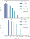 |
Fig. 1 Marginalised log10 probabilities for each of TOI-2076 c (upper) and TOI-2076 d (lower) period aliases, as computed by MonoTools before CHEOPS observations. |
2 Data
2.1 TESS observations
TESS observed TOI-2076 in sectors 16 and 23 in 2-min cadence. We use the TESS light curves created by H21 to supplement the CHEOPS data, which are explained in more detail in H21, Sect. 2.1. These light curves use the target pixel file (TPF) products from the SPOC pipeline from sectors 16 and 23. Cadences with significantly poor data quality are removed. Light curves are built taking the pipeline aperture, and detrended using lightkurve’s RegressionCorrector tool (Cardoso et al. 2018). The final composite light curve is detrended against a linear combination of (i) significant trends of pixels outside the aperture, (ii) the mean and standard deviation of the mission quaternions, and (iii) a b-spline. Together these components remove scattered light background, jitter and stellar variability, respectively. Cadences expected to contain transits were masked in this fit. This produces a light curve which has improved precision over the pipeline products, as can be seen in H21, Figs. 1 and 2.
2.2 CHEOPS observations
Through the CHEOPS Guaranteed Time Observations (GTO) programme CH_PR110048 (“Duos – Recovering long period duo-transiting planets”), we scheduled multiple observations of period aliases for TOI-2076 c and d. The observing strategy was dictated by determining the marginal probability for each alias (described in Sect. 3.2) and observing aliases with p > 2%. The strategy was then adapted for each new observation we received.
In total this led to a single visit of a TOI-2076 c period alias, and two visits of TOI-2076 d period aliases. Detailed information for each Cheops visit and ground-based photometric observation is shown in Table 1. We also re-observed a transit of the inner planet, TOI-2076 b, to improve radius precision and potentially detect transit timing variations (TTVs).
The CHEOPS data were processed by the most recent Data Reduction pipeline DR13 (Hoyer et al. 2020). We downloaded CHEOPS data from DACE (Buchschacher et al. 2015) using the pycheops interface (Maxted et al. 2021), and chose the decontaminated OPTIMAL light curve. We then clipped outliers, using both the in-built pycheops default function, and then a further step to clip any points with a background value larger than 0.2, or a flux outside of the range of −5 < (flux/ppt) < 5. We also extracted important decorrelation parameters including centroid position, background, roll-angle, smear, etc. The raw and detrended CHEOPS data presented here is available through CDS.
Scheduling continuous transit observations at high-efficiency is a complex problem and, due to competition between the many targets and programmes on CHEOPS, not all planned observations can typically be observed. This meant CHEOPS did not cover all high-probability period aliases for TOI-2076 d and was unable to recover a period, leaving possible aliases at 25.1 and 35.1 d. Therefore, in order to confirm the orbital period, we turned to ground-based observatories.
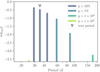 |
Fig. 2 Marginalised log10 probabilities for TOI-2076 d period aliases, as computed by MonoTools after the detection of the P = 21 d alias of TOI-2076 c and before CHEOPS observations of TOI-2076 d. The log probability of the P = 25.1 d alias is far below the y axis limit with log10 p = −19.59. |
2.3 LCO/McDonald observations
We observed a transit window of the 25.09 d alias of TOI-2076 d in Pan-STARRS z-short band on UTC 2021 May 05 from the Las Cumbres Observatory Global Telescope (LCOGT or LCO; Brown et al. 2013) 1.0m network node at McDonald Observatory. We used the TESS Transit Finder, which is a customised version of the Tapir software package (Jensen 2013), to schedule our transit observations. The 1 m class telescopes are equipped with 4096 × 4096 pixel SINISTRO cameras having an image scale of 0.389″ per pixel, resulting in a 26′ × 26′ field of view. Exposures were defocused to improve efficiency and photometric precision. The images were calibrated by the standard LCOGT BANZAI pipeline (McCully et al. 2018), and photometric data were extracted using AstroImageJ (Collins et al. 2017). The images have a typical stellar point-spread-function with a FWHM of ~5″, and circular photometric apertures with radius 7.4″ were used to extract the differential photometry. The target star photometric aperture excludes flux from the nearest Gaia EDR3 neighbours. Raw and detrended LCO/McDonald photometry is available on CDS.
2.4 SAINT-EX observations
In an effort to catch the 35.1 d alias of planet d, TOI-2076 was observed on the night of 2021-05-25 between 03:17 and 06:29 UT from the SAINT-EX telescope at the San Pedro Mártir observatory, Mexico (Demory et al. 2020). SAINT-EX is a 1-metre F/8 Ritchey-Chretien telescope built to be complementary to the SPECULOOS network of telescopes, which are focused on searching for transiting planets around ultra-cool dwarfs (Sabin et al. 2018; Sebastian et al. 2021).
Due to its 12′ field of view, it was not possible to include any bright comparison stars in the same field as TOI-2076. The observations were made using the r′ filter. In order to increase the efficiency and avoid saturation of the bright target, the telescope was defocused, producing a ringed PSF with a diameter of ~10 pixels.
We performed simple image reduction and extracted source counts for TOI-2076 and 7 comparison stars using AstroImageJ (or AIJ), setting an aperture with a radius of 30 pixels, and extracting background flux from an annulus between 47 and 58 pixels in distance from each source. As well as total fluxes for each star, we also extracted meta-data including airmass, PSF width, PSF FWHM, X and Y centroids, PSF roundness, which were used to help decorrelate the light curve. Raw and detrended Saint-Ex photometry is available on CDS.
2.5 LCO/MuSCAT observations
A Director’s Discretionary Time proposal on the LCOGT network was also approved to observe and confirm the P = 35.1 d alias. An ingress of this alias was visible from Haleakala, Hawaii on 2021-06-29 (BJD=2459394.95), and we scheduled a 4.8 h observation of TOI-2076 with the MuSCAT-3 instrument on the 2.0 m Faulkes Telescope North (Narita et al. 2020). The MuSCAT-3 instrument is able to simultaneously observe in g, r, i and z filters at different exposure lengths, enabling photometric observations with high efficiency (Narita et al. 2015). Due to the bright nature of TOI-2076, we opted to perform the observations with the diffuser in place, thereby allowing longer exposures without assymetric PSFs caused by defocusing. We used exposure times of 37, 19, 21 and 25 s respectively and the FAST read-out mode, resulting in 405, 647, 701, and 605 exposures respectively.
The small field of view of MuSCAT-3 meant that no similar-brightness stars were present within the field. Extraction was performed using a combination of AstroImageJ and the MuSCAT-3 pipeline1.
The MuSCAT-3 pipeline produced aperture photometry with less scatter and therefore we used this as our flux input. The “entropy” parameter computed by the pipeline (flux inside the photometry aperture normalised by the total aperture flux) was also extracted as a useful detrending parameter. From the AIJ analysis, we extracted the more complete meta-data, including sum of comparison star flux, PSF width, x and y centroids, etc. Raw and detrended LCO/MuSCAT-3 photometry is available on CDS.
Key information for all of the photometry presented in this paper.
3 Analysis
3.1 Stellar parameters
Derived stellar parameters are shown in Table 2.
3.1.1 Bulk physical properties
In order to derive precise stellar parameters, we used spectra taken with HARPS-N at Telescopio Nazionale Galileo, in the framework of the Global Architecture of Planetary Systems (GAPS) project (see e.g. Covino et al. 2013; Carleo et al. 2020). 64 spectra taken between 2020-08-06 and 2021-06-14 were co-added into a single stacked spectrum which had an average S/N of around 650 at 550 nm. We then derived the stellar atmospheric parameters (Teff, log g, microturbulence, [Fe/H]), and its respective uncertainties using ARES+MOOG, following the same methodology described in Santos et al. (2013) and Sousa (2014). We measured the equivalent widths (EW) of iron lines using the ARES code2 (Sousa et al. 2007, 2015). A minimisation process was used to find the ionisation and excitation equilibrium once it converges to the best set of spectroscopic parameters. This process uses a grid of Kurucz model atmospheres (Kurucz 1993) and the radiative transfer code MOOG (Sneden 1973). We obtained a temperature of 5200 ± 70 K, a log g of 4.45 ± 0.12 dex, a [Fe/H] of −0.09 ± 0.04, and a microturbulance velocity of 1.08 ± 0.05 km s−1.
To compute the stellar radius of TOI-2076, we used a modified infrared flux method (IRFM; Blackwell & Shallis 1977) to determine the stellar angular diameter and effective temperature via a Markov-chain Monte Carlo (MCMC) approach, as recently detailed in Schanche et al. (2020). As these properties can be derived from the stellar apparent bolometric flux, we produce synthetic photometry by constructing spectral energy distributions (SEDs) from stellar atmospheric models using the stellar parameters derived from our spectral analysis as priors that we attenuate to account for reddening with the extinction left as a free parameter. The computed synthetic fluxes were compared with the retrieved broadband fluxes and uncertainties from the most recent data releases for the following bandpasses; Gaia G, GBP, and GRP, 2MASS J, H, and K, and WISE W1 and W2 (Skrutskie et al. 2006; Wright et al. 2010; Gaia Collaboration 2021). To include any systematic uncertainties derived from stellar atmospheric model differences in our stellar radius error we used a Bayesian modelling averaging method with stellar models from a range of ATLAS (Kurucz 1993; Castelli & Kurucz 2003) catalogues in order to produce weighted averaged posterior distributions. From this analysis we find a Teff and E(B − V) of 5181 ± 37 K and 0.02 ± 0.01, respectively. Lastly, we converted the stellar angular diameter of TOI-2076 to the radius using the offset corrected Gaia EDR3 parallax (Lindegren et al. 2021), and obtain a Rs = 0.7699 ± 0.0059 R⊕.
The set given by (Teff, [Fe/H], Rs) is then assumed as input to derive the isochronal mass Ms and age ts. To this end, we used the isochrone placement technique (Bonfanti et al. 2015, 2016) applied to pre-computed grids of PARSEC3 v1.2S (Marigo et al. 2017) isochrones and tracks to compute a first pair of mass and age estimates. Furthermore, we derived a second pair of mass and age values by directly fitting the input set into the evolutionary tracks built by the CLES4 code (Scuflaire et al. 2008), following the Levenberg-Marquadt minimisation scheme presented in Salmon et al. (2021). Our adopted  M⊙ and
  Gyr values are finally computed by merging the two respective pairs of distributions inferred from the two different evolutionary models, after checking their mutual consistency using the χ2-based criterion described in detail in Bonfanti et al. (2021). The derived parameters are in agreement (at the 1 σ level) with those derived by H21.
3.1.2 Stellar Age
H21 presented multiple lines of evidence for the youth of both TOI-2076 and TOI-1807, a separate transiting planet host close-by and co-moving with TOI-2076 which likely formed together. This included gyrochronology (125−230 Myr), log R′HK (12− 870 Myr), Li absorption (<800 Myr), Ca II IR triplet core emission (<1000 Myr) and X-ray flux (>18 Myr), giving a combined age of 200 ± 50 Myr. We chose to re-assess the age given our follow-up spectra and more precise stellar parameters.
We derived the Mount Wilson Ca II index (log R′ HK – the chromospheric contribution of the H and K Ca lines) from the stacked HARPS-N spectra of −4.373 ± 0.02 using ACTIN (Gomes da Silva et al. 2018). The relation of Lorenzo-Oliveira et al. (2016) allows us to convert this to a stellar age of 0.42 ± 0.13 Gyr – far more precise than that of H21. We also re-derived a gyrochronological age using the relation of Mamajek & Hillenbrand (2008) and the rotation period derived by H21 (6.84 ± 0.58d), finding a slightly older age of 0.25 ± 0.12 Gyr. Both these techniques therefore support a young (<0.5 Gyr) age, and are in agreement with the independent analyses presented in H21. We adopt the weighted mean of the two activity-derived ages as our derived age of TOI-2076 going forward − 0.34 ± 0.08 Gyr.
These stellar ages are at odds with that derived from our isochrones, which is imprecise but suggests an intermediate-age star  . However, isochronal ages are frequently in tension with astroseismology and activity-derived ages (e.g. Pont & Eyer 2005; Brown 2014; Kovács 2015), therefore we choose not to include it in our derived average age.
Derived stellar parameters.
3.2 Photometry: TESS-only analysis
In order to determine which aliases to observe, we first performed model fits to the available TESS transits. Typically transit modelling relies on a known orbital period in order to constrain not just the orbital parameters, but also those parameters which determine the transit shape, such as the transit duration and impact parameter, which are influenced by orbit through limits on the planetary velocity. In our case, such constraints need to be inverted – we must use the transit shape to constrain the orbital velocity (and therefore orbital period). With this goal in mind, we developed the MonoTools package, which is able to model transit lightcurves in cases of multiple transits, duotransits and monotransits, as well as multiple systems with combinations of such candidates, with both radial velocities and transit photometry5.
For such fits, impact parameter, transit duration, and radius ratio are fitted together in a way that is agnostic of the exoplanet orbit. The combination of these transit shape parameters, along with a stellar density constrained from stellar parameters, implies a unique transverse planetary velocity. In the inverse case – where transit shape constrains orbital parameters – this is known as the photoeccentric effect (e.g. Dawson & Johnson 2012). Converting this velocity directly to a single orbital period parameter and trimming the samples to those regions round period aliases would be incredibly inefficient as the vast majority of derived orbital periods would not fall within these discreet period alias “island”. So instead, MonoTools calculates a marginalised probability distribution across all allowed aliases for a given transit model by combining priors for each alias.
A major part of this is the period prior of P−8/3 as derived by Kipping (2018). This is necessary as short-period orbits are highly favoured over long-period ones due to a combination of geometric probability and window function. Secondly, a prior is calculated using the probability of the implied orbital velocity given some prior eccentricity distribution. Exoplanet population studies show that planets, especially in multi-planet systems, have a general distribution that peaks at low eccentricities. These population-derived distributions (e.g. Kipping 2013; Van Eylen & Albrecht 2015) also imply a probability distribution of orbital velocities relative to the velocity of a circular orbit. This is because velocities much faster or much slower than that of a circular orbit are disfavoured as they imply highly eccentric orbits, which exoplanet population studies show are uncommon (Kipping 2013), especially in short-period (P < 100 d) multi-planet systems (Van Eylen & Albrecht 2015). Instead of performing this step analytically (which requires a complex and infeasible integration over the eccentricity prior), MonoTools uses pre-computed interpolations for the velocity prior calculated numerically.
The boost to geometric transit probability for eccentric orbits, and the effect of a maximum eccentricity are also considered in this interpolated function. In the case of a multi-planet system, orbits which graze (i.e. enter the Hill spheres of) interior planets can be rejected and therefore provide a maximum eccentricity. We use a simple 3-part logmass-radius relation derived from fitting observed exoplanets in order to compute Hill spheres on-the-fly. By modelling all planets simultaneously, the inner planet transits can also improve knowledge of the stellar density, hence improving the derived orbital parameters from transit shape.
For TOI-2076, we used the eccentricity distribution of Van Eylen & Albrecht (2015), as this is applicable to short-period transiting multi-planet systems as observed by TESS. We also included a Gaussian Process with a simple harmonic oscillator kernel (SHOTerm) using celerite (Foreman-Mackey et al. 2017; Foreman-Mackey 2018) which was pre-trained on out-of-transit data, and has quality factor set to  , which is typical for stellar noise. The resulting posterior probabilities for each period alias are found in Fig. 1.
We then found the highest-probability aliases which together would give us a ≳90% probability of a transit redetection. These were then scheduled on CHEOPS, with the highest-probability aliases of each planet being given highest priority in the CHEOPS scheduler. This was a total of 5 TOI-2076 c aliases and 4 TOI-2076 d aliases.
After the detection of a unique period for TOI-2076 c, we re-performed this analysis, the resulting marginalised probability distributions are shown in Fig. 2. The presence of a planet on a 21 d orbit interior to planet d drastically reduced the probability of the inner-most alias due to MonoTools rejecting orbits intersecting with the Hill sphere of TOI-2076 c. We updated our CHEOPS observations accordingly, focusing on aliases between 29 and 45 d.
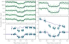 |
Fig. 3 TESS (upper panels) and CHEOPS (lower panels) individual transits of planets b and c. In the two lower panels, we show both the extracted CHEOPS flux with the best-fit decorrelation model (offset above), and the detrended CHEOPS flux with the best-fit transit model (below). |
3.3 Final combined model
CHEOPS data unambiguously detected a unique P = 21.0154 d period for TOI-2076 c (see the lower right panel of Fig. 3). For TOI-2076 d, we have observed all aliases shorter than P = 87.8 d using either CHEOPS or ground-based facilities. The CHEOPS observations on 2021-04-29 and 2021-05-13 clearly ruled out the 43.9 d alias, and 29.27 d and 58.54d aliases, respectively (see second and fourth panels of Fig. 4). Ground-based observations from LCO/McDonald covered the 25.1 d alias, while photometry from both Saint-Ex and LCO/MuSCAT-3 covered the 35.1 d alias.
As our TESS-only models showed, the probabilities of periods longer than 80 d (87.8 d and 175.6 d) are extremely low compared to close-in orbits due to both the period priors, and to the eccentricity priors derived from the transit shape. The geometric and temporal period prior alone gives an 87.8 d orbit a probability 28 times lower than that at 25.1 d, while that at 175.6 d is 179 times lower. For comparison the 35.1 d orbit is disfavoured by only a factor 2.5.
We can therefore probabilistically exclude these longer orbits as well as those ruled out by CHEOPS observations and focus only on the two short-period aliases for which we have ground-based observations – those at 25.1 and 35.1 d.
Our final combined model therefore has two goals – provide accurate planetary parameters for all three planets, and determine the true period of the available planets. To do this, we modelled all available photometry simultaneously, including transit models for all three planets and detrending parameters. For the competing period aliases, we built two models with identical parameters and changed only the period of TOI-2076 d. The relative difference in log likelihood can then be used for model selection, as the models otherwise share the same number of parameters and datapoints.
The size of the model means co-fitting the TESS light curve with a GP was not possible, therefore in order to remove residual systematic noise and/or stellar activity from the TESS light curve we subtracted a spline function fitted to the out-of-transit data and extrapolated over the transits. We also masked outliers with flux 4σ away from both preceding and succeeding points, and masked all points more than 3.5 transit durations from all transits to improve computational speed.
The combined model was built using PyMC3 (Salvatier et al. 2016), which performs Hamiltonian Monte Carlo sampling - a far more efficient sampling technique than Markov Chain, as it can use the local gradient of the likelihood function to quickly move to distant regions of parameters space, even if correlated. Transit models used the exoplanet package (Foreman-Mackey et al. 2021a).
As our model contained 108 independent parameters, many of which included correlations, we were only able to sample the model thanks to first using the sampler provided with exoplanet (which is able to learn and explore off-diagonal covariances), and second by providing independent parameter groups on which to compute these covariances (namely, groups of detrending parameters for each telescope)6. We ran each model with eight 3500-sample chains after a burn-in of 12 000 steps to produce 28 000 samples. We verified the gelmin-rubin statistic (R) was below 1.05, that the effective sample size was a large fraction of the total steps (>10000), and that the traces of individual chains were suitably mixed and Gaussian.
3.3.1 Treatment of CHEOPS data
CHEOPS photometry can retain trends due to systematics, and previous works present in detail the techniques used to correct for these (e.g. Bonfanti et al. 2021; Delrez et al. 2021; Maxted et al. 2021). We chose to co-fit the photometric transit models with a decorrelation against certain parameters. These included the x and y components of the roll angle sin Φ and cos Φ, as well as estimates of background, CCD smear flux, and the change in temperature (ΔT). We also included both a linear and quadratic decorrelation component against time in order to model the stellar variability apparent in the CHEOPS lightcurves. Past Cheops results (e.g. Delrez et al. 2021; Maxted et al. 2021) have opted to further detrend as a function of roll-angle using for example a spline or Gaussian process fit, however our inspection of the Cheops flux residuals as a function of roll-angle for each visit revealed no apparent additional variations that would require such additional (and computationally intensive) modelling.
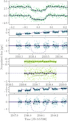 |
Fig. 4 Observations of TOI-2076 d, including unsuccessful transit observations. Upper panel: The two TESS transits detected by H21 as well as our best-fit model from the combined model. Two mid-upper panels: A CHEOPS observation covering the 43.9 d alias. Two mid-lower panels: A LCO/McDonald lm Sinistra lightcurve of the 25.09 d alias. Lower panel: A CHEOPS observation covering both 29.27 d and 58.54 d aliases. In the lower three panels, a TOI-2076 d model-fit is shown to demonstrate the expected transit shape and depth. In the lower three plots, the upper points and line show the raw flux and best-fit decorrelation model, while the lower panel shows the detrended flux and the expected transit model. |
3.3.2 Treatment of ground-based data
The majority of our ground-based observations are both affected by airmass trends and a lack of comparison stars. On average, TOI-2076 provides 15 times more photons that all comparison stars combined, therefore relative photometry is dominated by the shot noise of comparison stars. Instead we decided to use the raw aperture photometry and decorrelate against parameters linked to likely systematics.
Flux measurements with values 4σ above or below both their neighbours were masked. In the case of MuSCAT-3 data, three differential colour time-series were derived using the normalised fluxes for all stars (target and comparisons) between neighbouring filters (e.g. g/r, r/i, i/z). We fitted a spline with 15-minute knot spacing to each of the four normalised flux time-series (weighted by inverse photometric uncertainty), allowing us to interpolate differential colour estimates between each of the bands despite the asynchronous spacing of the four MuSCAT-3 detectors. Given this is a confirmed multi-planet system without any nearby stellar companions, we can make the assumption that the transit depth should be unchanged across all filters, and therefore colour is independent of the transit. This does not completely hold for limb-darkening, however this is a secondary effect with the maximum difference in transit shapes between lightcurves being 120 ppm and the average being only 50 ppm – an order of magnitude smaller than the transit depth. As this effect is dependent on a transit occurring, it cannot itself introduce a transit shape, and can only bias the derived parameters. Given the noise inherent in our ground-based data compared to e.g. the TESS transits, model parameters can only be minimally biased by this effect on the data. Therefore including colour information (which directly constrains colour-related systematics) as a linear decorrelation parameter results in a net improvement in the quality of the MuSCAT data and the general fit.
To find the important detrending parameters, we first included a wide array of parameters in a local model including airmass, time, x and y centroid, width, full width half-maximum (FWHM), total comparison flux, and g/r, r/i and i/z (for Muscat-3). These were normalised such that their medians were at 0.0 and the 1-sigma region spanned −1 to 1. We then iterated multiple models, removing detrending parameters that resulted in statistically insignificant gradients. The priors and posteriors for these detrending parameters are shown in Tables B.1 and B.2.
Ground-based photometry (raw and detrended) will also be made available through CDS.
3.3.3 Treatment of limb darkening
We used the quadratic limb darkening parameters for all six bandpasses available. In each case, we used theoretical limb darkening parameters calculated by Claret (2021) for CHEOPS, Claret (2018) for TESS, and Claret & Bloemen (2011) for g, r, i, and z bandpasses. In each case, we fitted a 2D interpolation surface to both u1 and u2 parameters as a function of Teff and log g. Then, using samples of TOI-2076 stellar parameters, the resulting distribution of limb darkening parameters were used to form a normal prior input to the transit models, although we rounded the prior standard deviation to 0.05 to avoid over-fitting.
3.4 TTV analysis
Rather than fitting for a specific fixed period, our combined model fitted transits individually using a normal prior centred on the expected time of transit given a linear ephemeris and a loose standard deviation of 0.025 d (36 min). These outputs revealed clear TTVs, with the CHEOPS transit of TOI-2076 b arriving 57 ± 5 min early compared to a linear ephemeris using only the TESS data, while TOI-2076 c arrived 50 ± 4 min late. This can be seen in Fig. 5. TTVs are also expected given the period ratios of the planets are close to period commensurability.
To analyse the observed TTVs and ensure confidence in our results, we performed independent TTV analyses using three distinctly different approaches. The same derived transit times and errors were then used as input to these analyses. As the SAINT-EX ground-based lightcurve of TOI-2076 d has a low S/N, it is excluded from the TTV analysis.
We performed three approaches - one using the TTVfaster package (Agol & Deck 2016) and Ultranest Nested Sampling (Buchner 2021b), and two using the approach presented in Leleu et al. (2021b) which used the TTVf ast algorithm (Deck et al. 2014), and the samsam7 MCMC algorithm (see Delisle et al. 2018). For full details of these fits, see Appendix A. The output of the first model (TTVfaster/Ultranest) is shown purely for reference in Fig. 5.
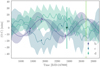 |
Fig. 5 Observed TTVs and TTVFaster/Ultranest TTV models for each of the three planets. Coloured lines show the median best-fit TTV models, while coloured regions show 1 -σ range. The predicted transit time for the low S/N SAINT-EX observation of planet d is shown as a triangle with white edges, while the observed transit time is shown with dark-edged inverted triangles. Planned TESS observations of the two planets in 2022 are shown in light green. |
3.5 Orbital stability analysis
In order to test the compatibility of the two remaining high-probability aliases at 25.1 d and 35.1 d with the 21 d period of TOI-2076 c, we performed an N-body stability analysis. We used the rebound8 package (Rein & Liu 2012) with the whfast integrator (Rein & Tamayo 2015) and we activated the Mean Exponential Growth factor of Nearby Orbits (MEGNO, Cincotta & Simó 2000) indicator. The orbital configuration can be considered stable when the value of MEGNO is close to 2 (Cincotta & Simó 2000). We compute the masses using forecaster9 from the planetary radii and stellar mass and radius. We used the radii values of planet b and c determined in Sects. 3.2 and 3.3, we assumed an error of 0.5 R⊕ on radius of the planet d. We drew 1000 values of masses between the lower and upper boundaries provided by forecaster, and assumed uniform distribution of the mean anomaly (between 0 and 2π), for each planet. We fixed the eccentricity to 0, argument of pericenter to 90°, and the longitude of the ascending node to 180°, for each planet. We sampled 500 values of the period of the planet d for each of the two possible aliases, from two Gaussian distribution centred at 25.09 d and 35.126 d, both with a standard deviation of 0.1 d – chosen to be larger than both the period uncertainties (<0.0001 d) and the observed TTVs (0.02 d) to guard against systematic uncertainties. The inclinations and periods have been assumed normally distributed with the values and uncertainties obtained from the analysis described in Sects. 3.2 and 3.3. We ran 1000 simulations and we integrated the orbits for 100 000 years with a step-size of 0.25 d. We assigned a value of the MEGNO indicator ≫ 2 if the system underwent a close encounter or if a body gained a semi-major axis greater than 150 au.
4 Results
4.1 Combined model
The derived planetary parameters from our combined model can be seen in Table 3. We find planetary radii of 2.518 ± 0.036, 3.497 ± 0.043, and 3.232 ± 0.063 R⊕, respectively, which are significantly smaller than those of H 21 which found 3.282 ± 0.043, 4.438 ± 0.046, and 4.14 ± 0.07 R⊕. The main reason for this appears to be due to a bug in the modelling performed in H21 where the radius ratio (Rp/Rs) was submitted to exoplanet’s LimbDarkLightCurve function, rather than the radii in solar units (Rp/R⊙). This led to final radius values that were inflated by a factor of R⊙/RS ~ 1.31. Hence, the radii and radius ratios defined here should supersede those in H21.
As shown in Sect. 3.3, CHEOPS photometry clearly reveals the True period of TOI-2076c to be  . All period aliases shorter than 87.8 d were observed either with CHEOPS or from the ground. As shown in our TESS-only analysis (Sect. 3.2), the longest period aliases (87.8 d and 175.6 d) are orders of magnitude less likely due to constraints from the lightcurve as well as period and eccentricity priors. CHEOPS photometry clearly rules out the 29.27 d, 43.9 d and 58.54 d aliases. This left the 25.1 d and 35.1 d aliases for which we obtained ground-based photometric follow-up.
In order to assess the fit and implications of our model fits to each period alias, we computed the differences in log likelihoods, log priors and log probabilities in Table 4. As the number of data points and parameters are preserved across models, the difference in Bayesian information criterion (ΔBIC, Schwarz 1978) is simply ΔBIC = −2Δ log prob. Typically ΔBIC > 10 or Δ log prob < −5 is used to show strong support for a model (Raftery 1995).
Our combined model clearly prefers the 35.1 d alias as opposed to the 25 and 88 d aliases, as can be seen from the derived log probability differences in Table 4. When combined with the log-priors derived from the combination of geometric, window function and eccentricity priors derived in our TESS-only modelling, we find Δ log prob values of more than 150 in favour of the P = 35.1 d model. We therefore adopt this as the true period of TOI-2076 d, although we further discuss the orbit of TOI-2076 in 5.1.
4.2 TTVs
We find for the first time that the TOI-2076 system exhibits large TTVs with amplitudes greater than 20 minutes for planets b and c. However, our three approaches to modelling the TTVs each find inconsistent planetary masses (see Table A.1 and Appendix A). This implies that the number of transit timing measurements is not yet sufficient to obtain robust mass estimates from TTVs and, as expected for a model without strong constraints from the data, the choice of prior modifies the resulting posteriors, as can be seen in the determined masses and eccentricities in Table A.1. We therefore caution use of those parameters derived from TTVs (i.e. planetary mass) until more transits can be observed, although we use the TTVFaster/Ultranest results (which have the most realistic prior distributions and output masses) as representative masses for future calculations (e.g. TSM).
The best-fitting models do appear to suggest a significant anti-correlated TTV signal between planets b and c, due to their proximity to the 2:1 mean motion resonance creating a 713.1 ± 2.7 d super-period. The relationship between planets c and d is not well defined due to the number of transits, but our best-fit TTV models suggest that long-term sinusoidal TTVs between planets c and d could be observed in the future, as well as a potential chopping signal that could allow for precise mass measurements.
Derived planetary parameter posterior distributions for each of the three planets.
Log probabilities for each of the remaining aliases.
4.3 Orbital stability
We found the 5.3 ± 1% of the simulations around the 25.1-d-alias are stable (MEGNO ~ 2), while the 89 ± 1.4% of the simulations (445 out of 500) around the 35-d-alias are stable. These results indicate that the 35-d-alias is the most favourable period for the planet d.
5 Discussion
5.1 The orbit of TOI-2076 d
In Table 4, we revealed the differences in log probabilities between three difference period aliases. The major difference in log likelihood are driven by the presence and absence of transits in ground-based follow-up data. The TESS data, which only allowed for identifying the original period aliases, consequently show near-identical transit models and log-likelihoods. For the 25 d case the loglikelihoods are the result of a transit in the LCO/McD data, but a flat line in the MuSCAT3 data; the 35 d case is the loglikelihood of a flat line in the LCO/McD data and a transit in MuSCAT3; while the 88 and 176 d aliases show the loglikelihood of flat lines in each of the ground-based transits.
The largest difference in log likelihood (~100) comes from the LCO/MuSCAT-3 observations. Despite the fact that the LCO/MuSCAT-3 data required substantial detrending with respect to colour and airmass, the transit model was far better able to explain the sharp ingress feature at BJD = 2459395.87 compared to linear detrending, which occurred precisely at the expected transit time given a linear ephemeris (upper panels, Fig. 6). The SAINT-EX data, which was lower S/N and covers only a very short duration of in-transit data, is not as conclusive as the LCO/MuSCAT-3 data, although the transit model is also marginally preferred in this dataset (lower panel, Fig. 6).
The second reason for the better model (a difference of ~75 in log likelihood) fit is the non-detection of a transit using the LCO/1m data from McDonald observatory during a purported transit of the Pd = 25 d alias. The observation, which occurred at low airmass and covered the entire expected transit event, appears to see no clear flux drop, and a flat model is preferred over a transit one (lower panel, Fig. 4).
This hypothesis is also supported by our orbital stability analysis – where the vast majority of long-term orbits for the Pd = 35.1 d alias are stable, and those of the Pd = 25.1 d orbit are not. However, the Pd = 25.1 d scenario could be stable if planets c and d were caught in an MMR, for example the 6:5 configuration which, although less common than the 5:3 ratio implied by the Pd = 35.1 d, is not impossible (e.g. the Kepler-36 system Carter et al. 2012). Such a possibility seems less likely given the potentially disturbing influence of the inner  planet (which, as discussed in Sect. 3.4, is not in resonance), and given the fact that the observed TTV of planet c appears satisfactorily explained by anti-correlation with the TTVs of planet b, rather than due to the influence of any closer-proximity outer planet.
The 35.1 d alias also appears more likely when considering the orbital periods of the system. Planets b and c are close to but slightly outside of a 2:1 period ratio (2.03). Such a pile-up of planets just beyond period ratios is common in multi-planet systems and may be a hallmark of disc migration (Fabrycky et al. 2014). The 35.1d alias follows that trend by being extremely close but just outside of a 5:3 orbital ratio with planet c (5.014:3). None of the other potential period aliases show this pattern, although the P = 25.08936 d alias is just inside a 6:5 ratio (5.969:5).
Taken together, we believe the evidence for a 35.1 d period for TOI-2076 d is compelling and we hereafter refer to it as the correct period.
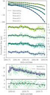 |
Fig. 6 Ground-based observations of the 35.1 d alias of TOI-2076 d. Upper panel: Raw LCO/MuSCAT-3 observations of TOI-2076 in four filters. Middle panel: Detrended lightcurves in the four filters, along with best-fit transit models. Lower panels: Raw (upper) and detrended (lower) SAINT-EX photometry along with a best-fit transit model. |
5.2 Planetary characteristics
Thanks to our determination of planetary periods, we now know that the TOI-2076 planets are irradiated by 84, 32, and 16 S⊕ respectively. Compared to many sub-Neptunes so-far detected, this is remarkably low and suggests that the effect of stellar insolation on e.g. their radii must be minimal. From the radii alone, we can say that all of the three TOI-2076 planets likely have extended H-He atmospheres. These inflated radii may in part be explained by their youth. Young planets are affected by a handful of processes which could change their bulk physical parameters. The first is photo-evaporation, however with a star of age 340 ± 80 Myr and orbits of >0.05 AU, this is likely no longer a dominant effect except potentially for planet b. Also important is the process of core-powered mass-loss by which small planets with light gaseous envelopes can lose their outer layers through thermal heating by the cooling core (Ginzburg et al. 2018). Finally, atmospheric contraction may still be acting on the TOI-2076 planets (e.g. Lopez et al. 2012). Berger et al. (2020) explored differences in radius populations as a function of planetary age, and found that the average radius of sub-Neptunes appears to shift with time from ~3.0 R⊕ at <1 Gyr to ~2.5 R⊕ at > 1 Gyr, particularly for planets with irradiation less than 150 S⊕ like TOI-2076 b, c, and d. With radii of Rc =3.497 ± 0.043 and Rd =3.232 ± 0.063 R⊕, the outer planets in the TOI-2076 system may provide evidence that young sub-Neptunes are born with even more inflated radii than the ~3.0 R⊕ seen in Berger et al. (2020). If puffy H-He envelopes are able to be maintained for hundreds of Myr, it could be a sign that core-powered mass loss and/or contraction are slower processes than previously thought. The atmospheres of the outer planets orbiting TOI-2076 could therefore be the perfect test-beds for such theories.
5.3 Future observations
TOI-2076 will be re-observed by TESS in Sector 50 (2022-Mar-26 to 2022-Apr-22; see Fig. 5). Although exact downlink gaps are not yet known, it is likely that b will show 3 transits, while both c and d will transit once. The timing of these transits will help further constrain TTVs for this system, and can be helped by a campaign of observations with CHEOPS, especially to observe sequential transits of c and d, thereby potentially detecting the predicted chopping signal and better constraining the masses of the three planets.
We predict expected RV semi-amplitudes of 1.88 ± 0.87, 1.62 ± 0.71, and  ms−1 using the provisional masses implied by our TTVFaster/Ultranest models (although we caution that robust TTV masses will require more transit observations). This would make these three planets extremely challenging targets, especially when considering the strong ~7d rotation signal present in the TESS light curve. Therefore, TTVs may prove the best method of constraining the planetary masses for the three planets around TOI-2076. Of the many small young planets detected by TESS, TOI-2076 hosts three of the most atmospherically accessible, all with transmission spectroscopy metrics (TSM; Kempten et al. 2018) above 100, although those values host large uncertainties due primarily to the large mass uncertainties. Indeed, if the mass of TOI-2076 c is confirmed to be 6.0 M⊕, it is amongst the highest-ranked cool and small planets with Teq < 750 K, Rp <4 R⊕ found by TESS. There are also very few small young planets with equivalently accessible atmospheres (see Fig. 7), with only the mini-Neptunes around AU Mic (Plavchan et al. 2020) and HD 63433 (TOI-1726, Mann et al. 2020) with similar TSM values, likely due to their host stars superior brightnesses (G = 7.8 and 6.7). Hence, the planets around TOI-2076 could form key targets for future atmospheric follow-up with e.g. the James Webb Space Telescope (JWST). Their long periods may also mean the outer planets are relatively unperturbed by stellar radiation pressure or wind, enabling the planets to maintain large exospheres which may be detectable in the UV with e.g. the STIS or COS instruments on the Hubble Space Telescope.
6 Conclusions
We performed targeted follow-up photometry of the period aliases of the young, long-period sub-Neptunes TOI-2076 c and d in order to confirm their orbital periods and further characterise the system. We initially modelled the planetary system using MonoTools, developed specifically for this task, which is able to take available stellar and photometric data and calculate a marginal probability for each period alias.
Using ESA’s CHEOPS space telescope, we performed targeted follow-up of the highest-probability aliases and were able to confirm the  d period alias as the true one for TOI-2076 c. CHEOPS observations also helped rule out three of the most-probable period aliases for TOI-2076 d. Ground-based photometry from the 1-meter LCO/Sinistro telescope at McDonald Observatory enables us to discard one of the remaining high-probability aliases for TOI-2076 d at 25.1 d, which is also hinted at by stability and TTV analyses of this alias in the presence of the 21.0154 d TOI-2076 c. Furthermore, ground-based observations with both the 2-meter LCO/MuSCAT-3 on the Faulkes North telescope at Haleakala and the 1-meter SAINT-EX telescope at San Pedro Martir were able to detect ingresses of the 35.1 d alias. Bayesian model comparison vastly favoured this alias over the other unexcluded aliases (A log p > 100), confirming 35.12537 ± 0.00067 d as the true period of TOI-2076 d.
With high-precision space-based transit observations spanning two years, thanks to TESS and CHEOPS, we were able to improve the ephemerides and radius precision, with updated radii of Rb =2.518 ± 0.036, Rc =3.497 ± 0.043, and Rd =3.232 ± 0.063 R⊕. These transits also enabled us to detect anti-correlated TTVs between TOI-2076 b and c with an amplitude of ~30 min, although TTV modelling did not have enough observed transits to constrain masses and eccentricities. The three planets inflated radii suggest all three are low-density warm sub-Neptunes with significant hydrogen envelopes, potentially still undergoing atmospheric contraction. Their large radii, low incident flux and bright host star magnitude make all three planets extremely interesting targets for future atmospheric characterisation with e.g. IWST.
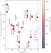 |
Fig. 7 Comparison of transmission spectroscopy metrics for all small transiting planets (Rp < 5 R⊕) around young stars (age < 500 Myr) as a function of age in million years (Myr). Point size represents planetary radius, while point colour shows equilibrium temperature. Multi-planet systems with small planets are connected by red trails. The TOI-2076 system is labelled in red with TSM calculated using tentative masses derived from our TTVFaster/Ultranest models. |
Acknowledgments
Acknowledgements. We thank the anonymous referee for a thorough and constructive review. CHEOPS is an ESA mission in partnership with Switzerland with important contributions to the payload and the ground segment from Austria, Belgium, France, Germany, Hungary, Italy, Portugal, Spain, Sweden, and the United Kingdom. The CHEOPS Consortium would like to gratefully acknowledge the support received by all the agencies, offices, universities, and industries involved. Their flexibility and willingness to explore new approaches were essential to the success of this mission. This work has been carried out within the framework of the NCCR PlanetS supported by the Swiss National Science Foundation. This material is based upon work supported by the National Science Foundation through the US Community Open Access to LCO facilities provided under Grant No. 2034337. This paper is based on observations made with the MuSCAT3 instrument, developed by Astrobiology Center and under financial supports by JSPS KAKENHI (JP18H05439) and JST PRESTO (JPMJPR1775), at Faulkes Telescope North on Maui, HI, operated by the Las Cumbres Observatory. This research made use of exoplanet (Foreman-Mackey et al. 2021a,b) and its dependencies (Agol et al. 2020; Kumar et al. 2019; Astropy Collaboration 2013, 2018; Kipping 2013; Luger et al. 2019; Salvatier et al. 2016; Theano Development Team 2016). This work makes use of observations from the LCOGT network. Part of the LCOGT telescope time was granted by NOIRLab through the Mid-Scale Innovations Program (MSIP). MSIP is funded by NSF. AT acknowledges support from an STFC PhD studentship. This work has been carried out within the framework of the NCCR PlanetS supported by the Swiss National Science Foundation. DG and LMS gratefully acknowledge financial support from the Cassa di Risparmio di Torino (CRT) foundation under Grant No. 2018.2323 “Gaseousor rocky? Unveiling the nature of small worlds”. SGS acknowledges the support from FCT through Investigador FCT contract nr. CEECIND/00826/2018 and POPH/FSE (EC). This work was supported by FCT – Fundacçâo para a Ciência e Tecnologia through national funds and by FEDER through COMPETE2020 – Programa Operacional Competitividade e Internacionalizaçâo by these grants: PTDC/FIS-AST/32113/2017 and POCI-01-0145-FEDER-032113; PTDC/FIS-AST/28953/2017 and POCI-01-0145-FEDER-028953; PTDC/FISAST/28987/2017 and POCI-01-0145-FEDER-028987. ACC and TGW acknowledge support from STFC consolidated grant numbers ST/R000824/1 and ST/V000861/1, and UKSA grant ST/R003203/1. VVG is a FRS-FNRS Research Associate. The Belgian participation to CHEOPS has been supported by the Belgian Federal Science Policy Office (BELSPO) in the framework of the PRODEX Program, and by the University of Liège through an ARC grant for Concerted Research Actions financed by the Wallonia-Brussels Federation. LBo, GPi, VNa, GSs, IPa, and RRa acknowledge the funding support from Italian Space Agency (ASI) regulated by “Accordo ASI-INAF n. 2013-016-R.O del 9 luglio 2013 e integrazione del 9 luglio 2015 CHEOPS Fasi A/B/C”. MIH and YA acknowledge the support of the Swiss National Fund under grant 200020_172746. ML acknowledges support of the Swiss National Science Foundation under grant number PCEFP2J94576. ABr was supported by the SNSA. B-OD acknowledges support from the Swiss National Science Foundation (PP00P2-190080). PM acknowledges support from STFC research grant number ST/M001040/1. This work is partly financed by the Spanish Mnistry of Economics and Competitiveness through grants PGC2018-098153-B-C31 Acknowledges support from the Spanish Mnistry of Science and Innovation and the European Regional Development Fund through grant PGC2018-098153-B-C33, as well as the support of the Generalitat de Catalunya/CERCA programme. This project was supported by the CNES MG is an FRS-FNRS Senior Research Associate. GyMSz acknowledges the support of the Hungarian National Research, Development and Innovation Office (NKFIH) grant K-125015, a a PRODEX Experiment Agreement No. 4000137122, the Lendület LP2018-7/2021 grant of the Hungarian Academy of Science and the support of the city of Szombathely. This work was granted access to the HPC resources of MesoPSL financed by the Region Ile de France and the project Equip@Meso (reference ANR-10-EQPX-29-01) of the programme Investissements dAvenir supervised by the Agence Nationale pour la Recherche LD is an FRS-FNRS Postdoctoral Researcher. MF gratefully acknowledge the support of the Swedish National Space Agency (DNR 65/19, 174/18). This work was supported by FCT - Fundaçâo para a Ciência e a Tecnologia through national funds and by FEDER through COMPETE2020 – Programa Operacional Competitividade e Internacionalizaçâo by these grants: UID/FIS/04434/2019, UIDB/04434/2020, UIDP/04434/2020, PTDC/FIS-AST/32113/2017 and POCI-01-0145-FEDER-032113, PTDC/FIS-AST/28953/2017 and POCI-01-0145-FEDER-028953, PTDC/FIS-AST/28987/2017 and POCI-01-0145-FEDER-028987, ODSD is supported in the form of work contract (DL 57/2016/CP1364/CT0004) funded by national funds through FCT. We acknowledge support from the Spanish Mnistry of Science and Innovation and the European Regional Development Fund through grants ESP2016-80435-C2-1-R, ESP2016-80435-C2-2-R, PGC2018-098153-B-C33, PGC2018-098153-B-C31, ESP2017-87676-C5-1-R, MDM-2017-0737 Unidad de Excelencia Maria de Maeztu-Centro de Astrobiología (INTA-CSIC), as well as the support of the Generalitat de Catalunya/CERCA programme. The MOC activities have been supported by the ESA contract No. 4000124370. XB, SC, DG, MF and JL acknowledge their role as ESA-appointed CHEOPS science team members. This project has received funding from the European Research Council (ERC) under the European Union’s Horizon 2020 research and innovation programme (project Four Aces; grant agreement no. 724427); DE acknowledges financial support from the Swiss National Science Foundation for project 200021_200726. (covered by Tom Wilson’s acknowledgement) This work was also partially supported by a grant from the Simons Foundation (PI Queloz, grant number 327127). SH gratefully acknowledges CNES funding through the grant 837319. KGI is the ESA CHEOPS Project Scientist and is responsible for the ESA CHEOPS Guest Observers Programme. She does not participate in, or contribute to, the definition of the Guaranteed Time Programme of the CHEOPS mission through which observations described in this paper have been taken, nor to any aspect of target selection for the programme. YGMC is supported by UNAM-PAPIIT-IG101321. This work includes observations with SAINT-EX carried out at the Observatorio Astronómico Nacional on the Sierra de San Pedro Mártir (OAN-SPM), Baja California, México. SS have received funding from the European Research Council (ERC) under the European Unions Horizon 2020 research and innovation programme (grant agreement no. 833925, project STAREX).
Appendix A TTV modelling
We performed three TTV modelling approaches to derive planetary parameters and assess how prior-dependent these models are. In the first approach, we used the TTVfaster package (Agol & Deck 2016) to generate models of TTVs given input parameters for the three planets & star. TTVfaster requires the assumption that the planets are not in perfect resonant orbits with one another. Using the periods and epochs, we find that this assumption appears to be satisfied for b & c (Pc/Pb = 2.0296), but we cannot be sure about c & d, which are closer to a resonant ratio (Pd/Pc = 1.6713 = 5.0140/3).
As we had many parameters and few transit times with which to constrain them (which could result in multi-modal parameter space), we used a nested sampling approach which is better able to explore non-Gaussian parameter space than a simple MCMC (Buchner 2021a). We used Ultranest for this implementation (Buchner 2021b), and used the stepsampler.RegionSliceSampler method as the number of parameters is large.
For period and inclination priors, we used outputs from our combined model as Gaussian priors, but increased the standard deviation by a factor of 2.5 to limit any over-fitting. The best-fit transit epoch from the combined model was used as a normal prior, with a standard deviation of 0.05 d (far larger than the timing fit uncertainty to prevent overfitting). The longitude of ascending node and an argument of periastron were given wide uniform priors from −π to π. For eccentricity we used the halfnormal distribution of multi-planet systems from Van Eylen & Albrecht (2015) (σ = 0.096). Although typical samplers such as MCMC struggle due to correlations when not exploring e cos ω & e sin ω, we found this had little effect on our nested sampling results, likely because samples are independent from their predecessors. For the outer planets we reparameterised planetary masses as log mass ratios and planetary periods as simple ratios to avoid strong correlations (for planet b, as a ratio to the star, and for planets c & d as a ratio of planet b). For planetary mass ratios, we used the population of exoplanets with well-constrained masses and radii (Downloaded from the NASA exoplanet archive, Akeson et al. 2013) to produce broad Gaussian priors on log planetary mass (log Mp) given a planetary radius. This resulted in mass priors of  ,
,  and
and  for planets b, c & d respectively, which match very closely the predictions of forecaster(Chen & Kipping 2016). We inflated these standard deviations from the log Mp population prior by 0.1 to prevent overly constraining priors.
Indepedently, and in an effort to estimate the influence of the mass and eccentricity priors on the determined posterior − and to take into account the possible resonant motion of the outer pair (c and d are very close to the exact commensurability: Pd/Pc − 5/3 = 0.0047) − we use the approach presented in Leleu et al. (2021b). Here we estimated transit timing variations are estimated using the TTVfast algorithm (Deck et al. 2014), and the samsam10 MCMC algorithm (see Delisle et al. 2018) is used to sample the posterior. Following (Hadden & Lithwick 2017), we test the robustness of TTV mass-estimation by trying out two mass priors: log10-uniform and uniform. The mass and eccentricity posteriors are shown in Table A.1.
As shown in Table A.1, the determined masses depend strongly on the used priors. The nested sampling approach appears to find low but plausible masses for all three planets: Mb = 5.9 ± 2.8, Mc = 6.4 ± 2.9, and  M⊕. Best-fit TTV models from this approach are shown in Fig 5. However planets c & d may be in 5:3 resonance, in which case the models of TTVFaster are not valid. In addition, the inner pair is close, but not inside, a mean motion resonance, which creates degeneracy between the determined masses and eccentricities (Lithwick et al. 2012). The Leleu et al. (2021b) approach finds extremely small (Mp < 1M⊕) and large (Mp > 10M⊕) for the log-uniform & uniform mass priors respectively.
Priors and posteriors for planetary masses and eccentricities from each of the three TTV models used.
Appendix B Combined model parameters
Model parameters, priors, and posteriors for the Combined model.
Appendix C TTV Faster model parameters
Model parameters, priors and posteriors for the TTV faster/Ultranest TTV model.
References
- Agol, E., & Deck, K. 2016, TTVFaster: First order eccentricity transit timing variations (TTVs), Astrophysics Source Code Library [record ascl:1684.812] [Google Scholar]
- Agol, E., Luger, R., & Foreman-Mackey, D. 2020, AJ, 159, 123 [Google Scholar]
- Akeson, R.L., Chen, X., Ciardi, D., et al. 2013, PASP, 125, 989 [CrossRef] [Google Scholar]
- Astropy Collaboration (Robitaille, T.P., et al.) 2013, A&A, 558, A33 [NASA ADS] [CrossRef] [EDP Sciences] [Google Scholar]
- Astropy Collaboration (Price-Whelan, A.M., et al.) 2018, AJ, 156, 123 [NASA ADS] [CrossRef] [Google Scholar]
- Becker, J.C., Vanderburg, A., Rodriguez, J.E., et al. 2019, AJ, 157, 19 [Google Scholar]
- Benatti, S., Nardiello, D., Malavolta, L., et al. 2019, A&A, 630, A81 [NASA ADS] [CrossRef] [EDP Sciences] [Google Scholar]
- Benz, W., Broeg, C., Fortier, A., et al. 2021, Exp. Astron., 51, 109 [Google Scholar]
- Berger, T.A., Huber, D., Gaidos, E., van Saders, J.L., & Weiss, L.M. 2020, AJ, 160, 108 [NASA ADS] [CrossRef] [Google Scholar]
- Blackwell, D.E., & Shallis, M.J. 1977, MNRAS, 180, 177 [NASA ADS] [CrossRef] [Google Scholar]
- Bonfanti, A., Ortolani, S., Piotto, G., & Nascimbeni, V. 2015, A&A, 575, A18 [NASA ADS] [CrossRef] [EDP Sciences] [Google Scholar]
- Bonfanti, A., Ortolani, S., & Nascimbeni, V. 2016, A&A, 585, A5 [NASA ADS] [CrossRef] [EDP Sciences] [Google Scholar]
- Bonfanti, A., Delrez, L., Hooton, M.J., et al. 2021, A&A, 646, A157 [NASA ADS] [CrossRef] [EDP Sciences] [Google Scholar]
- Brown, D.J.A. 2014, MNRAS, 442, 1844 [NASA ADS] [CrossRef] [Google Scholar]
- Brown, T.M., Baliber, N., Bianco, F.B., et al. 2013, PASP, 125, 1031 [NASA ADS] [CrossRef] [Google Scholar]
- Bryant, E.M., Bayliss, D., Santerne, A., et al. 2021, MNRAS, 504, L45 [NASA ADS] [CrossRef] [Google Scholar]
- Buchner, J. 2021a, Annals of Statistics, submitted [arXiv:2181.89675] [Google Scholar]
- Buchner, J. 2021b, J Open Source Softw., 6, 3001 [NASA ADS] [CrossRef] [Google Scholar]
- Buchschacher, N., Ségransan, D., Udry, S., & Diaz, R. 2015, in Astronomical Society of the Pacific Conference Series, Astronomical Data Analysis Software an Systems XXIV (ADASS XXIV), eds. A.R. Taylor, & E. Rosolowsky, 495, 7 [NASA ADS] [Google Scholar]
- Cardoso, J.V.d.M., Hedges, C., Gully-Santiago, M., et al. 2018, Astrophysics Source Code Library, [record ascl:1812.813] [Google Scholar]
- Carleo, I., Malavolta, L., Lanza, A.F., et al. 2020, A&A, 638, A5 [NASA ADS] [CrossRef] [EDP Sciences] [Google Scholar]
- Carter, J.A., Agol, E., Chaplin, W.J., et al. 2012, Science, 337, 556 [NASA ADS] [CrossRef] [Google Scholar]
- Castelli, F., & Kurucz, R.L. 2003, in IAU Symposium, 210, Modelling of Stellar Atmospheres, eds. N. Piskunov, W.W. Weiss, & D.F. Gray, A20 [Google Scholar]
- Chen, J., & Kipping, D. 2016, ApJ, 834, 17 [Google Scholar]
- Cincotta, P.M., & Simö, C. 2000, A&As, 147, 205 [NASA ADS] [CrossRef] [EDP Sciences] [Google Scholar]
- Claret, A. 2018, VizieR Online Data Catalog: J/A+A/618/A20 [Google Scholar]
- Claret, A. 2021, Res. Notes Am. Astron. Soc., 5, 13 [NASA ADS] [Google Scholar]
- Claret, A., & Bloemen, S. 2011, A&A, 529, A75 [NASA ADS] [CrossRef] [EDP Sciences] [Google Scholar]
- Collins, K.A., Kielkopf, J.F., Stassun, K.G., & Hessman, F.V. 2017, AJ, 153, 77 [NASA ADS] [CrossRef] [Google Scholar]
- Cooke, B.F., Pollacco, D., Lendl, M., Kuntzer, T., & Fortier, A. 2020, MNRAS, 494, 736 [CrossRef] [Google Scholar]
- Cooke, B.F., Pollacco, D., Anderson, D.R., et al. 2021, MNRAS, 500, 5088 [Google Scholar]
- Covino, E., Esposito, M., Barbieri, M., et al. 2013, A&A, 554, A28 [NASA ADS] [CrossRef] [EDP Sciences] [Google Scholar]
- Cutri, R.M., Skrutskie, M.F., van Dyk, S., et al. 2003, VizieR Online Data Catalog: II/246 [Google Scholar]
- Dawson, R.I., & Johnson, J.A. 2012, ApJ, 756, 122 [NASA ADS] [CrossRef] [Google Scholar]
- Deck, K.M., Agol, E., Holman, M.J., & Nesvorny, D. 2014, ApJ, 787, 132 [CrossRef] [Google Scholar]
- Delisle, J.B., Ségransan, D., Dumusque, X., et al. 2018, A&A, 614, A133 [NASA ADS] [CrossRef] [EDP Sciences] [Google Scholar]
- Delrez, L., Ehrenreich, D., Alibert, Y., et al. 2021, Nat. Astron., 5, 775 [NASA ADS] [CrossRef] [Google Scholar]
- Demory, B.O., Pozuelos, F.J., Gömez Maqueo Chew, Y., et al. 2020, A&A, 642, A49 [NASA ADS] [CrossRef] [EDP Sciences] [Google Scholar]
- Dholakia, S., Dholakia, S., Mayo, A.W., & Dressing, C.D. 2020, AJ, 159, 93 [NASA ADS] [CrossRef] [Google Scholar]
- Dragomir, D., Teske, J., Günther, M.N., et al. 2019, ApJ, 875, L7 [NASA ADS] [CrossRef] [Google Scholar]
- Espinoza, N. 2018, Res. Notes Am. Astron. Soc., 2, 209 [Google Scholar]
- Espinoza, N., Brahm, R., Henning, T., et al. 2020, MNRAS, 491, 2982 [NASA ADS] [Google Scholar]
- Fabrycky, D.C., Lissauer, J.J., Ragozzine, D., et al. 2014, ApJ, 790, 146 [NASA ADS] [CrossRef] [Google Scholar]
- Foreman-Mackey, D. 2018, Res. Notes Am. Astron. Soc., 2, 31 [NASA ADS] [Google Scholar]
- Foreman-Mackey, D., Agol, E., Ambikasaran, S., & Angus, R. 2017, AJ, 154, 220 [Google Scholar]
- Foreman-Mackey, D., Luger, R., Agol, E., et al. 2021a, J. Open Source Softw., 6, 3285 [NASA ADS] [CrossRef] [Google Scholar]
- Foreman-Mackey, D., Savel, A., Luger, R., et al. 2021b, https://doi.org/18.5281/zenodo.4737444 [Google Scholar]
- Gaia Collaboration (Brown, A.G.A., et al.) 2021, A&A, 649, A1 [NASA ADS] [CrossRef] [EDP Sciences] [Google Scholar]
- Ginzburg, S., Schlichting, H.E., & Sari, R. 2018, MNRAS, 476, 759 [CrossRef] [Google Scholar]
- Gomes da Silva, J., Figueira, P., Santos, N., & Faria, J. 2018, J. Open Source Soft., 3, 667 [CrossRef] [Google Scholar]
- Guerrero, N.M., Seager, S., Huang, C.X., et al. 2021, ApJS, 254, 39 [NASA ADS] [CrossRef] [Google Scholar]
- Hadden, S., & Lithwick, Y. 2017, AJ, 154, 5 [Google Scholar]
- Hedges, C., Hughes, A., Zhou, G., et al. 2021, AJ, 162, 54 [NASA ADS] [CrossRef] [Google Scholar]
- Hoyer, S., Guterman, P., Demangeon, O., et al. 2020, A&A, 635, A24 [NASA ADS] [CrossRef] [EDP Sciences] [Google Scholar]
- Huang, C.X., Burt, J., Vanderburg, A., et al. 2018, ApJ, 868, L39 [NASA ADS] [CrossRef] [Google Scholar]
- Jensen, E. 2013, Tapir: A web interface for transit/eclipse observability, Astrophysics Source Code Library [record ascl:1386.887] [Google Scholar]
- Kane, S.R., Yalçinkaya, S., Osborn, H.P., et al. 2020, AJ, 160, 129 [NASA ADS] [CrossRef] [Google Scholar]
- Kempton, E.M.R., Bean, J.L., Louie, D.R., et al. 2018, PASP, 130, 114401 [CrossRef] [Google Scholar]
- Kipping, D.M. 2013, MNRAS, 434, L51 [NASA ADS] [CrossRef] [Google Scholar]
- Kipping, D. 2018, Res. Notes Am. Astron. Soc., 2, 223 [Google Scholar]
- Kovâcs, G. 2015, A&A, 581, A2 [NASA ADS] [CrossRef] [EDP Sciences] [Google Scholar]
- Kumar, R., Carroll, C., Hartikainen, A., & Martin, O.A. 2019, J. Open Source Softw., 4, 1143 [NASA ADS] [CrossRef] [Google Scholar]
- Kurucz, R.L. 1993, SYNTHE spectrum synthesis programs and line data (Cambridge, MA: Smithsonian Astrophysical Observatory) [Google Scholar]
- Leleu, A., Alibert, Y., Hara, N.C., et al. 2021a, A&A, 649, A26 [NASA ADS] [CrossRef] [EDP Sciences] [Google Scholar]
- Leleu, A., Chatel, G., Udry, S., et al. 2021b, A&A, 655, A66 [CrossRef] [Google Scholar]
- Lindegren, L., Bastian, U., Biermann, M., et al. 2021, A&A, 649, A4 [EDP Sciences] [Google Scholar]
- Lithwick, Y., Xie, J., & Wu, Y. 2012, ApJ, 761, 122 [Google Scholar]
- Lopez, E.D., Fortney, J.J., & Miller, N. 2012, ApJ, 761, 59 [NASA ADS] [CrossRef] [Google Scholar]
- Lorenzo-Oliveira, D., Porto de Mello, G.F., & Schiavon, R.P. 2016, A&A, 594, L3 [NASA ADS] [CrossRef] [EDP Sciences] [Google Scholar]
- Luger, R., Agol, E., Foreman-Mackey, D., et al. 2019, AJ, 157, 64 [Google Scholar]
- Mamajek, E.E., & Hillenbrand, L.A. 2008, ApJ, 687, 1264 [CrossRef] [Google Scholar]
- Mann, A.W., Johnson, M.C., Vanderburg, A., et al. 2020, AJ, 160, 179 [NASA ADS] [CrossRef] [Google Scholar]
- Marigo, P., Girardi, L., Bressan, A., et al. 2017, ApJ, 835, 77 [Google Scholar]
- Maxted, P., Ehrenreich, D., Wilson, T., et al. 2021, MNRAS, 514, 77 [Google Scholar]
- McCully, C., Volgenau, N.H., Harbeck, D.-R., et al. 2018, SPIE Conf. Ser., 10707, 107070K [NASA ADS] [Google Scholar]
- Narita, N., Fukui, A., Kusakabe, N., et al. 2015, J. Astron. Telescopes Instrum. Syst., 1, 045001 [CrossRef] [Google Scholar]
- Narita, N., Fukui, A., Yamamuro, T., et al. 2020, SPIE Conf. Ser., 11447, 114475K [NASA ADS] [Google Scholar]
- Newton, E.R., Mann, A.W., Tofflemire, B.M., et al. 2019, ApJ, 880, L17 [NASA ADS] [CrossRef] [Google Scholar]
- Newton, E.R., Mann, A.W., Kraus, A.L., et al. 2021, AJ, 161, 65 [NASA ADS] [CrossRef] [Google Scholar]
- Plavchan, P., Barclay, T., Gagné, J., et al. 2020, Nature, 582, 497 [Google Scholar]
- Pont, F., & Eyer, L. 2005, in ESA Special Publication, The Three-Dimensional Universe with Gaia, eds. C. Turon, K.S. O'Flaherty, & M.A.C. Perryman, 576, 187 [NASA ADS] [Google Scholar]
- Raftery, A.E. 1995, Sociol. Methodol., 25, 111 [CrossRef] [Google Scholar]
- Rein, H., & Liu, S.F. 2012, A&A, 537, A128 [NASA ADS] [CrossRef] [EDP Sciences] [Google Scholar]
- Rein, H., & Tamayo, D. 2015, MNRAS, 452, 376 [Google Scholar]
- Ricker, G.R., Winn, J.N., Vanderspek, R., et al. 2015, J. Astron. Telescopes Instrum. Syst., 1, 014003 [Google Scholar]
- Rizzuto, A.C., Newton, E.R., Mann, A.W., et al. 2020, AJ, 160, 33 [NASA ADS] [CrossRef] [Google Scholar]
- Sabin, L., Gömez Maqueo Chew, Y., Demory, B.-O., Petrucci, R., & Saint-Ex Consortium. 2018, in 20th Cambridge Workshop on Cool Stars, Stellar Systems and the Sun, 59 [Google Scholar]
- Salmon, S.J.A.J., Van Grootel, V., Buldgen, G., Dupret, M.A., & Eggenberger, P. 2021, A&A, 646, A7 [NASA ADS] [CrossRef] [EDP Sciences] [Google Scholar]
- Salvatier, J., Wiecki, T.V., & Fonnesbeck, C. 2016, PeerJ Comput. Sci., 2, e55 [Google Scholar]
- Santerne, A., Malavolta, L., Kosiarek, M.R., et al. 2019, Nature Astronomy, submitted [arXiv:1911.87355] [Google Scholar]
- Santos, N.C., Sousa, S.G., Mortier, A., et al. 2013, A&A, 556, A150 [NASA ADS] [CrossRef] [EDP Sciences] [Google Scholar]
- Schanche, N., Hébrard, G., Collier Cameron, A., et al. 2020, MNRAS, 499, 428 [NASA ADS] [CrossRef] [Google Scholar]
- Schanche, N., Pozuelos, F.J., Günther, M.N., et al. 2022, A&A, 657, A45 [NASA ADS] [CrossRef] [EDP Sciences] [Google Scholar]
- Schwarz, G. 1978, Ann. Stat., 6, 461 [Google Scholar]
- Scuflaire, R., Théado, S., Montalbân, J., et al. 2008, Ap&SS, 316, 83 [NASA ADS] [CrossRef] [Google Scholar]
- Sebastian, D., Gillon, M., Ducrot, E., et al. 2021, A&A, 645, A100 [EDP Sciences] [Google Scholar]
- Skrutskie, M.F., Cutri, R.M., Stiening, R., et al. 2006, AJ, 131, 1163 [NASA ADS] [CrossRef] [Google Scholar]
- Sneden, C.A. 1973, PhD thesis, The University of Texas at Austin, USA [Google Scholar]
- Sousa, S.G. 2014, Determination of Atmospheric Parameters of B, A, F and G Type Stars (Springer), eds. E. Niemczura, B. Smalley, W. Pych, 297 [Google Scholar]
- Sousa, S.G., Santos, N.C., Israelian, G., Mayor, M., & Monteiro, M.J.P.F.G. 2007, A&A, 469, 783 [NASA ADS] [CrossRef] [EDP Sciences] [Google Scholar]
- Sousa, S.G., Santos, N.C., Adibekyan, V., Delgado-Mena, E., & Israelian, G. 2015, A&A, 577, A67 [NASA ADS] [CrossRef] [EDP Sciences] [Google Scholar]
- Sozzetti, A., Damasso, M., Bonomo, A.S., et al. 2021, A&A, 648, A75 [NASA ADS] [CrossRef] [EDP Sciences] [Google Scholar]
- Stassun, K.G., Oelkers, R.J., Pepper, J., et al. 2018, AJ, 156, 102 [NASA ADS] [CrossRef] [Google Scholar]
- Teske, J., Diaz, M.R., Luque, R., et al. 2020, AJ, 160, 96 [NASA ADS] [CrossRef] [Google Scholar]
- Theano Development Team. 2016, ArXiv e-prints, [arXiv: 1685.82688] [Google Scholar]
- Van Eylen, V., & Albrecht, S. 2015, ApJ, 808, 126 [Google Scholar]
- Wright, E.L., Eisenhardt, P.R.M., Mainzer, A.K., et al. 2010, AJ, 140, 1868 [NASA ADS] [CrossRef] [Google Scholar]
The last version of ARES code (ARES v2) can be downloaded at https://github.com/sousasag/ARES
Padova And TRieste Stellar Evolutionary Code: http://stev.oapd.inaf.it/cgi-bin/cmd
https://github.com/bmorris3/forecaster python3 version.
All Tables
Derived planetary parameter posterior distributions for each of the three planets.
Priors and posteriors for planetary masses and eccentricities from each of the three TTV models used.
Model parameters, priors and posteriors for the TTV faster/Ultranest TTV model.
All Figures
|
Fig. 1 Marginalised log10 probabilities for each of TOI-2076 c (upper) and TOI-2076 d (lower) period aliases, as computed by MonoTools before CHEOPS observations. |
| In the text | |
|
Fig. 2 Marginalised log10 probabilities for TOI-2076 d period aliases, as computed by MonoTools after the detection of the P = 21 d alias of TOI-2076 c and before CHEOPS observations of TOI-2076 d. The log probability of the P = 25.1 d alias is far below the y axis limit with log10 p = −19.59. |
| In the text | |
|
Fig. 3 TESS (upper panels) and CHEOPS (lower panels) individual transits of planets b and c. In the two lower panels, we show both the extracted CHEOPS flux with the best-fit decorrelation model (offset above), and the detrended CHEOPS flux with the best-fit transit model (below). |
| In the text | |
|
Fig. 4 Observations of TOI-2076 d, including unsuccessful transit observations. Upper panel: The two TESS transits detected by H21 as well as our best-fit model from the combined model. Two mid-upper panels: A CHEOPS observation covering the 43.9 d alias. Two mid-lower panels: A LCO/McDonald lm Sinistra lightcurve of the 25.09 d alias. Lower panel: A CHEOPS observation covering both 29.27 d and 58.54 d aliases. In the lower three panels, a TOI-2076 d model-fit is shown to demonstrate the expected transit shape and depth. In the lower three plots, the upper points and line show the raw flux and best-fit decorrelation model, while the lower panel shows the detrended flux and the expected transit model. |
| In the text | |
|
Fig. 5 Observed TTVs and TTVFaster/Ultranest TTV models for each of the three planets. Coloured lines show the median best-fit TTV models, while coloured regions show 1 -σ range. The predicted transit time for the low S/N SAINT-EX observation of planet d is shown as a triangle with white edges, while the observed transit time is shown with dark-edged inverted triangles. Planned TESS observations of the two planets in 2022 are shown in light green. |
| In the text | |
|
Fig. 6 Ground-based observations of the 35.1 d alias of TOI-2076 d. Upper panel: Raw LCO/MuSCAT-3 observations of TOI-2076 in four filters. Middle panel: Detrended lightcurves in the four filters, along with best-fit transit models. Lower panels: Raw (upper) and detrended (lower) SAINT-EX photometry along with a best-fit transit model. |
| In the text | |
|
Fig. 7 Comparison of transmission spectroscopy metrics for all small transiting planets (Rp < 5 R⊕) around young stars (age < 500 Myr) as a function of age in million years (Myr). Point size represents planetary radius, while point colour shows equilibrium temperature. Multi-planet systems with small planets are connected by red trails. The TOI-2076 system is labelled in red with TSM calculated using tentative masses derived from our TTVFaster/Ultranest models. |
| In the text | |
Current usage metrics show cumulative count of Article Views (full-text article views including HTML views, PDF and ePub downloads, according to the available data) and Abstracts Views on Vision4Press platform.
Data correspond to usage on the plateform after 2015. The current usage metrics is available 48-96 hours after online publication and is updated daily on week days.
Initial download of the metrics may take a while.