| Issue |
A&A
Volume 663, July 2022
|
|
|---|---|---|
| Article Number | A31 | |
| Number of page(s) | 10 | |
| Section | The Sun and the Heliosphere | |
| DOI | https://doi.org/10.1051/0004-6361/202142979 | |
| Published online | 08 July 2022 | |
Decayless longitudinal oscillations of a solar filament maintained by quasi-periodic jets⋆
1
School of Astronomy and Space Science, Nanjing University, Nanjing 210023, PR China
e-mail: chenpf@nju.edu.cn
2
Key Laboratory of Modern Astronomy and Astrophysics (Nanjing University), Ministry of Education, Nanjing 210023, PR China
3
Key Laboratory of Dark Matter and Space Astronomy, Purple Mountain Observatory, CAS, Nanjing 210033, PR China
Received:
22
December
2021
Accepted:
28
March
2022
Context. As a ubiquitous phenomenon, large-amplitude longitudinal filament oscillations usually decay in 1–4 periods. Recently, we observed a decayless case of such oscillations in the corona.
Aims. We try to understand the physical process that maintains the decayless oscillation of the filament.
Methods. Multiwavelength imaging observations and magnetograms were collected to study the dynamics of the filament oscillation and its associated phenomena. To explain the decayless oscillations, we also performed one-dimensional hydrodynamic numerical simulations using the code MPI-AMRVAC.
Results. In observations, the filament oscillates without decay with a period of 36.4 ± 0.3 min for almost 4 h before eruption. During oscillations, four quasi-periodic jets emanate from a magnetic cancellation site near the filament. The time interval between neighboring jets is ∼68.9 ± 1.0 min. Numerical simulations constrained by the observations reproduced the decayless longitudinal oscillations. However, it is surprising to find that the period of the decayless oscillations is not consistent with the pendulum model.
Conclusions. We propose that the decayless longitudinal oscillations of the filament are maintained by quasi-periodic jets, which is verified by the hydrodynamic simulations. More importantly, it is found that, when it is driven by quasi-periodic jets, the period of the filament longitudinal oscillations also depends on the driving period of the jets, not on the pendulum period alone. With a parameter survey in simulations, we derived a formula by which the pendulum oscillation period can be derived using the observed period of decayless filament oscillations and the driving periods of jets.
Key words: Sun: filaments / prominences / Sun: oscillations / Sun: atmosphere
Movie associated to Fig. 2 is available at https://www.aanda.org
© ESO 2022
1. Introduction
Solar prominences are bright cloud-like structures composed of plasmas with lower temperature and higher density than the ambient corona (e.g., Labrosse et al. 2010; Mackay et al. 2010; Parenti 2014; Vial & Engvold 2015; Gibson 2018). The typical plasma density of prominences is approximately 1010–1011 cm−3, and the typical temperature is approximately 104 K. When a prominence rotates from the solar limb to the solar disk, it is called a filament. This is typically visible at Hα, He I 10830 Å, extreme-UV (EUV), and radio wavelengths (e.g., van Ballegooijen 2004; Berger et al. 2010; Schmieder et al. 2010, 2014; Shen et al. 2015; Yan et al. 2015; Yang et al. 2017). Except for some filaments that are maintained by chromospheric siphon flows (e.g., Wang 1999) so that magnetic dips are not necessary (Karpen et al. 2001) for them, many filaments are thought to be supported by magnetic dips, which allow filament threads to be held in stable equilibrium with the upward Lorentz force balancing the gravity (Chen et al. 2020). The corresponding magnetic configurations with dips include sheared arcades (Kippenhahn & Schlüter 1957), magnetic flux ropes (Kuperus & Raadu 1974), or a combination of arcades and flux ropes (Guo et al. 2010; Liu et al. 2012).
A filament might exist for up to several days or months, during which it is continually disturbed by sporadic traveling waves, microflares, cold surges and hot jets, and by the everlasting convection on the solar surface. Once disturbed, a filament begins to oscillate. Filament oscillations can be classified into two categories (i.e., transverse oscillations (Hershaw et al. 2011; Dai et al. 2012; Shen et al. 2014b; Zhang & Ji 2018) and longitudinal oscillations (Jing et al. 2003; Luna et al. 2014; Shen et al. 2014a; Mazumder et al. 2020)). For both categories, observations indicate that filament oscillations generally damp out in 1–4 periods (Arregui et al. 2018) because of various dissipation mechanisms, such as radiative losses, thermal conduction, resonant absorption, and wave leakage. However, Chen et al. (2008) investigated the dynamics of a prominence with spectroscopic observations, and found that the prominence oscillations lasted for 4 h without damping. The prominence oscillated with two periods: 20 min and ∼60 min. Presumably, the shorter period corresponds to the transverse mode, and the longer period corresponds to the longitudinal mode. Because this decayless oscillation was followed by an eruption, they tentatively proposed that long-duration oscillations could be a precursor of prominence eruptions and coronal mass ejections (CMEs). Since then, an increasing number of observations have indicated that decayless oscillations of prominences or filaments are followed by eruptions (Gosain et al. 2009; Duchlev et al. 2010; Li & Zhang 2012; Mashnich & Bashkirtsev 2016; Mashnich & Kiselev 2019). More recently, Luna et al. (2018) conducted a survey of 196 filament longitudinal oscillation events in the first half of 2014 and found that while the distribution of the ratio of the decay time and the period peaks at 1.25 and most events damp out in three periods, a few events manifest long-term oscillations without significant damping or even with amplification. They also noted that these events are followed by eruptions.
These observations raise two important questions: (1) What is the mechanism to maintain the undamped or even amplified longitudinal oscillations in some filaments? (2) What is the relationship between the decayless prominence oscillations and ensuing prominence eruptions? In this paper, we study the umdamped event of filament longitudinal oscillation on 2014 July 5 in order to answer these two questions. The observations and data analysis are shown in Sect. 2. The observational results are described in Sect. 3. In Sect. 4, one-dimensional (1D) hydrodynamic simulations are performed to reproduce the observations, which is followed by discussions in Sect. 5. The main conclusions are summarized in Sect. 6.
2. Observations and data analysis
The left panel of Fig. 1 shows the local Hα image around the filament, which is located near active region (AR) 12104 on 2014 July 5. The Hα data were collected by the Kanzelhöhe Observatory. The line-of-sight magnetogram provided by the Helioseismic and Magnetic Imager (HMI) on board the Solar Dynamics Observatory (SDO) is overplotted on the Hα image, where the solid red and blue curves mark the contours of negative and positive magnetic field strength at different levels ranging from −50 G to 50 G. The filament spine is clearly visible and roughly distributed along the polarity inversion line (Martin 1990). After ∼18:30 UT on July 5, the filament started to oscillate. After oscillating for almost 4 h, the filament erupted and left a C3.8-class solar flare behind, which was registered by the GOES satellite (Chen et al. 2021). No CME is clearly identified in the Large Angle and Spectrometric COronagraph (LASCO) coronagraph observations, but a faint CME is detected by the COR2 coronagraph on board the Solar Terrestrial Relations Observatory (STEREO). The discrepancy probably results from the unfavorable observing vantage of LASCO since the source active region is close to the solar disk center in the LASCO field of view, whereas it is close to the limb in the STEREO field of view.
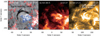 |
Fig. 1. Multiwavelength imaging observations on the AR filament. Panel a: corresponding Hα image of the filament provided by the Kanzelhöhe Observatory at 13:10:46 UT, where the red and blue contour lines represent different levels of magnetic field strength ranging from −50 G to 50 G. The arrow indicates a right-bearing barb of the filament. Panel b: SDO/AIA 304 Å image observed at 13:10:43 UT. Panel c: SDO/AIA 171 Å image observed at 23:19:36 UT. The arrows mark left-skewed flare loops formed after the filament eruption. |
The KSO Hα telescope has a spatial resolution of ∼2″ with a 2k × 2k CCD camera in operation (Steinegger et al. 2000), which is relatively low in revealing the fine structures of the oscillating filament. The evolution of the filament is also observed at multiple EUV wavelengths by the Atmospheric Imaging Assembly (AIA; Lemen et al. 2012) on board the SDO. The AIA data have a spatial resolution of ∼1 2 and a cadence of 12 s. We used only the 171 Å and 304 Å images. The Helioseismic and Magnetic Imager (HMI; Scherrer et al. 2012) on board the SDO provides photospheric magnetograms that can trace the associated evolution of the magnetic field on the solar surface. The AIA and HMI data are calibrated by using the standard solar software (SSW) routines aia_prep.pro and hmi_prep.pro. The full-disk Hα and AIA 304 Å images were coaligned using the cross-correlation method, and all images were derotated to a preoscillation time, that is, 18:35:12 UT. The right panel of Fig. 1 depicts the SDO/AIA 304 Å image taken at approximately the same time as the left panel. The EUV filament has a longer extension in the southern part, which is barely visible in Hα. This is a typical feature of filaments (Aulanier & Schmieder 2002).
3. Observational results
The filament has a quite long lifetime, existing in AR12104 from June 29 as a prominence above the east solar limb to July 5, when it is near the solar disk center. At ∼18:35 on July 5, the first jet emanates from nearby, moving toward the filament at a speed of 100.1 km s−1. The jet is manifested as bright emissions in 171 Å, and is accompanied by dark features, as displayed in panel (b) of Fig. 2, which depicts several snapshots of the filament evolution observed by SDO/AIA at 171 Å. In response to the impact of the jet, the filament starts to oscillate along the direction of its threads. Therefore, this oscillation is a typical longitudinal oscillation. The second and third jets emanate from the same site at 19:42 UT and 20:52 UT, respectively, causing the filament to oscillate with an almost constant amplitude. When the brightest fourth jet is ejected at 21:49 UT, the filament starts to erupt, leaving flaring loops in the low corona and flaring ribbons near the solar surface.
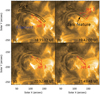 |
Fig. 2. Temporal evolution of the AR filament in AIA 171 Å from 18:35 UT to 22:20 UT. In panel a, a slice is chosen in order to plot the time-distance diagram in Fig. 3. The black arrow in panel b marks dark features accompanying the jets. The animation of this figure is available online. |
To show the sequence of the jets and the resulting filament oscillations, we selected a slice along the trajectory of the jets and along the filament threads, as bounded by the solid line in Fig. 2a. The positive direction of the slice was chosen from west to east so that the jet propagation is along the positive direction. In this case, the filament eruption, which is toward the west, would appear along the negative direction of the slice. The time-distance diagram of the 171 Å intensity distribution along the slice is plotted in Fig. 3, where the filament is located at a distance of 70″ in Fig. 3. Quasi-periodic jets are identified as the bright ridges extending from the position at ∼20″ in Fig. 3 to the edge of the filament, which are indicated by the dashed cyan lines. The slopes of the four bright ridges characterize the moving velocities of the jets, which are found to be 100.1, 100.1, 108.0 and 157.5 km s−1. The time interval between the first and second jet is approximately 67.9 min, that between the second and third jet is approximately 69.9 min, and that between the third and fourth jet is approximately 58.5 min. It is shown that the first and second time intervals are close to each other, and the third interval is slightly smaller, indicating that the jets are quasi-periodic. The period averaged by the first two intervals is 68.9 min. A fifth jet starts at 22:20 UT. However, it is not related to the filament oscillations because the filament has already risen rapidly. The properties of the quasi-periodic jets are listed in Table 1. In addition, the duration of each jet is ∼5 min. Figure 3 does not only show four quasi-periodic jets before the filament eruption, but also reveals continuous dark ridges along the trajectory with similar velocities. These absorptive ridges are thought to be cold surges, and they appear more frequently, even between successive hot jets.
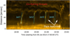 |
Fig. 3. Time-distance diagram of the AIA 171 Å intensity along the slice marked in Fig. 2a. The distance increases from west to east, therefore the dark ridge with a strong slope around 22:40 UT means that the filament was erupting toward the west. The figure indicates decayless filament oscillations associated with quasi-periodic jets. |
Parameters of the quasi-periodic jets observed by SDO/AIA.
To quantitatively investigate the oscillatory behavior of the filament, we zoom-in on Fig. 3 around the filament part, and the corresponding time-distance diagram is displayed in Fig. 4a. We find that the oscillatory behavior of the filament threads differs significantly from ordinary large-amplitude longitudinal oscillations which damp out in about three periods (Luna et al. 2018; Dai et al. 2021). The filament exhibits a decayless oscillation. To calculate the position of the filament thread at each time, we traced the upper and lower boundaries of the filament thread by the strongest intensity gradient along the slice direction because the dark filament is often bounded by a bright layer. We defined the middle point of the upper and lower boundaries as the centroid of the filament. The filament intensity distribution along the slice was fitted with a Gaussian profile in order to obtain the full width at half maximum (FWMH) absorption of radiation, which was then taken as the uncertainty of the centroid position (Awasthi et al. 2019). The evolution of the filament centroid is displayed in Fig. 4b. We used a decaying sine function of time to fit the temporal variation of the filament thread centroid, that is,
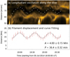 |
Fig. 4. Panel a: close-up view of Fig. 3 around the filament, highlighting the filament oscillations. Panel b: evolution of the filament centroid (red error bars) and the fitted curve (black line). |
where y0 and ϕ0 denote the initial position and phase angle of the oscillation, respectively. A0, P, and τ denote the initial amplitude, period, and damping time of the large-amplitude filament oscillation, respectively. The evolution of the filament longitudinal displacement with uncertainty was fitted with the Markov chain Monte Carlo method (Sharma 2017) with 100 fitting tests. As a result, the initial amplitude of filament oscillation is A0 = 4.0 ± 0.15 Mm, the period is 36.4 ± 0.3 min, and the damping time is 1013 min, which implies that the oscillation is identical to a decayless one. According to the pendulum model (Luna & Karpen 2012; Zhang et al. 2012), the period P is mainly related to the curvature radius R of the dipped magnetic field line by  , where g⊙ = 2.74 × 10² m s−2 is the gravitational acceleration near the solar surface. The curvature radius of the magnetic dip is estimated to be 33.3 ± 0.5 Mm.
Figure 2 and the associated animation show that the repetitive jets originate from the western side of the filament channel. After comparing the AIA 171 Å images and the HMI longitudinal magnetograms, we identify the location of the jet source in the HMI magnetogram, which is marked by the small red squares in Fig. 5. Figures 5a–d display the photospheric magnetograms at 18:36, 19:48, 20:48 and 21:48 UT. We find that inside the red boxes the positive and negative magnetic polarities approach each other, and magnetic cancellation occurs.
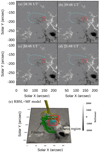 |
Fig. 5. Temporal evolution and nonlinear force-free field extrapolation model of the AR filament. Panels a–d: four snapshots of the SDO/HMI magnetogram around the filament channel, where white and black means positive and negative polarity, and the red squares correspond to the site of the jet source. The filament spine is represented by the dashed cyan lines. Panel e: coronal magnetic field reconstructed using the RBSL flux rope and magneto-frictional model. The green field lines represent the flux rope and the yellow lines indicate that the overlying magnetic field contains a fan-spine structure. The red cube corresponds to the red squares in the top four panels, where magnetic reconnection probably occurred. |
To understand the magnetic configuration of the jet formation, the coronal nonlinear force-free field (NLFFF) was reconstructed by using the magneto-frictional model (Guo et al. 2016a,b), where a flux rope is embedded in a potential field in advance (van Ballegooijen et al. 2000; van Ballegooijen 2004). The regularized Biot-Savart laws (RBSL) method ensures that the embedded flux rope is in internal equilibrium beforehand (Titov et al. 2018; Török et al. 2018; Guo et al. 2019, 2021). Then the magnetic field was relaxed to a force-free state. After 60,000 steps in our magneto-friction code, the force-free metric, Σ(J × B)i/(JB), dropped to approximately 0.3, indicating that the magnetic field approached the force-free state, where B is the magnetic field, and J is the current density.
Figure 5e displays the coronal magnetic field overplotted on the photospheric magnetogram around the filament channel. The magnetic field lines in cyan are sheared more strongly than the twisted field lines of the filament in green. Magnetic reconnection is expected to occur between the two parts. After this interchange reconnection, jets would propagate along the twisted magnetic field lines, and hit the filament threads.
4. Numerical simulations
Without additional energy supply, an oscillating filament would damp out in about three periods even under the effects of radiation and thermal conduction. According to the previous section, we argue that the decayless oscillations of the filament on 2014 July 5 are due to the impact of quasi-periodic jets, which push the filament threads repetitively. To confirm this conjecture, we performed 1D hydrodynamic numerical simulations as in our previous works (Xia et al. 2011; Zhang et al. 2012, 2013, 2020; Zhou et al. 2017).
The whole procedure consists of four steps: (1) Filament thread formation: A filament thread is formed in a prescribed 1D magnetic field via the chromospheric evaporation and coronal condensation mechanism. (2) Relaxation: After halting the localized heating at the footpoints, the filament thread naturally relaxes to a quasi-static equilibrium state. (3) Perturbations: Four episodes of impulsive heating are imposed at one footpoint of the magnetic field line, which excite high-speed jets hitting the filament, resulting in filament longitudinal oscillations. The details are presented below.
4.1. Simulation setup
As described by Xia et al. (2011), we numerically solved the following 1D hydrodynamic equations of single-fluid fully ionized plasma:

where ρ, T, and v are the basic physical parameters (i.e., plasma density, temperature, and velocity). The plasma density is related to the number density of protons by ρ = 1.4mpnH, when helium is considered in the solar corona. Correspondingly, the plasma pressure is formulated as p = 2.3nHkBT. For the mono-atomic ideal gas, the specific heat ratio is γ = 5/3, hence the internal energy is described as ε = ρv2/2 + p/(γ − 1). In the above equations, g∥(s) is the component of gravity along the flux tube at a distance s. In addition, H(s) is set as the local heating, and Λ(T) is the optically thin radiation loss function. Spitzer heat conductivity is taken to be κ = 10−6T5/2 ergs cm−1 s−1 K−1. These equations were numerically solved with the open-source code, MPI-AMRVAC1 (Keppens et al. 2012; Xia et al. 2018). The numerical scheme HLL was adopted as the Riemann solver and we used a three-level mesh refinement, reaching the highest spatial resolution of 40.5 km.
As mentioned in Sect. 1 and in Chen et al. (2020), magnetic dips exist in many filaments, although not in all, as implied by the prevalence of filament longitudinal oscillations. For the filament in this study, on the one hand, longitudinal oscillations are observed, which implies that the filament is supported by magnetic dips. On the other hand, the filament has right-bearing barbs, and the flaring loops are left-skewed relative to the magnetic neutral line, implying negative helicity of the magnetic system. According to the method proposed by Chen et al. (2014), the filament is identified to be supported by a magnetic flux rope, rather than a sheared arcade. Hence, magnetic dips indeed exist in this filament. As illustrated in Fig. 6, we study the motion of the plasma along a dipped magnetic flux tube that is composed of the following parts: (1) a vertical segment extending to a height of s1 = 18 Mm from each footpoint to the corona; (2) two symmetrical quarter circles with a length of s2 = 7.48 Mm as the shoulders of the dipped magnetic field line; (3) in the middle part, there is a straight uniform helix, which is expressed as follows:
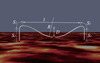 |
Fig. 6. Geometry of the flux tube in our simulations, where the central part is a helix described by Eq. (5). The natural coordinate is along the tube starting from the left footpoint. |
where l is the axis length of the helix and D is the radius of the magnetic flux tube, which is also equal to the dip depth. We set l = 90.5 Mm and D = 16.6 Mm, so that the resulting curvature radius of the magnetic dip would be R = 33.3 Mm, the same as derived from the observations in the previous section based on the pendulum model.
A steady background heating Hb = E0e−(s − smin)/λ + E0e−(smax − s)/λ was imposed to maintain the hot corona. Localized heating was then symmetrically imposed at the two footpoints so as to form a filament thread near the magnetic dip. After the localized heating was halted, the filament thread was relaxed for 5.5 h in order to reach a quasi-static equilibrium state. Because we adopted the optically thin radiation loss for the whole dynamics of the filament from formation to oscillation, the core temperature of the filament remained at ∼17 000 K, which is consistent with previous works (e.g., Karpen et al. 2006). In this case, the plasma was fully ionized in our simulated filaments. In reality, the core temperature of filaments is several thousand Kelvin, and the plasma is partially ionized, with the ionization rate being about 0.3 (Labrosse et al. 2010). Fortunately, even in the partially ionized situation, it was verified that a single-fluid assumption as used in this paper is still valid (Terradas et al. 2015).
To mimic the periodic jets, four heating pulses were then applied successively at the left footpoint of the magnetic flux tube with the same intervals as in the observations, which are listed in Table 1. Similar to Zhang et al. (2020), the impulsive heating Hi is expressed as follows:
![$$ \begin{aligned} H_i(s)=E_1 \exp {\left[{-\frac{(s-s_{\rm peak})^2}{s_{\rm width}^2}-\frac{(t-t_{\rm peak})^2}{t_{\rm scale}^2}}\right]}, \end{aligned} $$](/articles/aa/full_html/2022/07/aa42979-21/aa42979-21-eq8.gif)
where the spatial distribution is the same for various jets with speak = 6 Mm and swidth = 3 Mm, determined from the AIA 171 Å images. The damping time of the impulsive heating was 5 min for all the four thermal pulses. All pulses were set with the impulsive heating rate E1 = 4.4 × 10⁻³ erg cm−3 s−1.
To investigate the effects taken by the periodic thermal pulses, we also set up a control case, where only the first thermal pulse was introduced to cause the filament to oscillate. Its results were compared to those in the case with multiple pulses.
4.2. Simulation results
The top row of Fig. 7 displays the evolution of the temperature distributions in the control case (top left panel) and in the multipulse case (top right panel), where the blue segment in the middle around s = 80 Mm corresponds to the filament thread. In the control case, the filament thread begins to oscillate after being impinged by a single jet. The oscillation damps away quickly, as expected. In the multipulse case, in contrast, the filament thread oscillates continually. Before the oscillation is damped out, a second jet comes in, so the oscillation is amplified again.
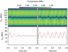 |
Fig. 7. Top row: time-distance diagrams of the temperature distribution along the magnetic flux tube in the control case (left) and in the multipulse case (right). Bottom row: temporal evolution of the displacement of the filament thread center in the control case (left) and in the multipulse case (right), where the dashed black lines correspond to the simulation results, and the solid red lines correspond to the fitting curves. |
In order to quantitatively compare the two cases, we extracted the position of the filament thread center at each time in each case, and its evolution is displayed as dashed black lines in the bottom row of Fig. 7, where the bottom left panel corresponds to the control case, and the bottom right panel corresponds to the multipulse case. The displacement evolution was fitted with a decaying sine function y = y0 + A0e−t/τsin(2πt/P + ϕ0), so that we can derive all the oscillation parameters, including the oscillation period (P) and decay time (τ). With the least-squares method, we fit the simulation results with the solid red lines in the bottom row of Fig. 7. The period is 36.4 min in the control case and 34.35 min in the multipulse case, and the damping time is 72.7 min in the control case and 5.2 × 10⁸ min (almost infinity) in the multipulse case. The fitting results are listed in Table 2. Surprisingly, we found that the periods are different between the control case and the multipulse case, and only in the control case is the oscillation period consistent with the pendulum model.
Parameters of simulated filament oscillations in the control case and the multipulse case.
5. Discussions
5.1. How filament decayless oscillations are maintained
Filament oscillations are a ubiquitous phenomenon in the solar atmosphere. With the existence of radiative cooling, heat conduction, and other dissipation processes, these oscillations generally damp out within about three periods. However, filament oscillations are occasionally decayless for a long time, which was proposed to be one of the precursors for filament eruptions or CMEs (Chen et al. 2008). The decayless behavior implies that additional energy must be supplied to the filament somehow. In this paper, we revealed that filament decayless oscillations are accompanied by quasi-periodic jets. Our 1D hydrodynamic simulations confirmed that quasi-periodic jets from the low corona hit the filament thread, maintaining the decayless longitudinal oscillations of the filament.
Solar jets are prevalent, which can be observed in solar active regions (Shibata et al. 1992, 1994; Yang et al. 2011; Chen et al. 2017; Shen et al. 2017), quiet-Sun regions and even coronal holes (Chen et al. 2012; Tian et al. 2014), with typical velocities in the range of 30–300 km s−1. They have been well explained to be due to magnetic reconnection either in the low corona or in the chromosphere. As illustrated in Fig. 5, the EUV jets in this paper indeed originate from a magnetic cancellation site near the eastern end of the filament channel. The approaching and canceling positive and negative magnetic polarities imply that the reconnection occurs in the low solar atmosphere, for instance, in the upper chromosphere. This is consistent with the coexistence of bright and dark EUV jets, which means that if the reconnection occurred in the low corona, only hot and bright EUV jets would be visible. Based on the photospheric magnetogram and the EUV images showing coronal loops and jet trajectories, the magnetic structure and connectivity are sketched in Fig. 8, where the dashed line corresponds to the magnetic neutral line, the black lines are the envelope magnetic field lines overlying the filament, the green line represents the magnetic field lines supporting the filament, and the cyan line corresponds to the low-lying strongly sheared field lines. The spatial relation between the green line and the cyan line is derived from the extrapolated coronal magnetic configuration with the same color-coding as in Fig. 5e.
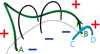 |
Fig. 8. Schematic sketch of the magnetic reconnection process, which triggers both repetitive jets and the onset of the filament eruption. The green line AB represents the magnetic field supporting the filament, and the cyan line CD represents the neighboring strongly sheared field line. The interchange reconnection between lines AB and CD leads to jets and to the expansion of the post-reconnection field line AD. |
As footpoints B and C are dragged to approach each other by the photospheric convection flows, interchange reconnection is triggered between field lines AB and CD. After reconnection, the green field line is rooted at point D with a concave-upward kink structure above footpoint D. While the smaller reconnected loop BC sinks down, producing the magnetic cancellation phenomenon, the upward reconnection outflow forms an EUV jet, moving along the post-reconnection field line AD. A bundle of magnetic field lines is involved in the reconnection process. For the field lines threading the filament, the jet directly hits the filament to oscillate longitudinally, as indicated by observations (Luna et al. 2014; Zhang et al. 2017; Zhang 2020) and illustrated by numerical simulations in this paper in 1D or in Luna & Moreno-Insertis (2021) in 2.5D. For the field lines encircling the filament, the jet plasma does not impact the filament material directly. Instead, the magnetic rearrangement after reconnection would impose a pulse on the filament, and the filament would begin to oscillate as well. This process can only be simulated only in 2D or 3D.
The above-mentioned jet-induced filament oscillations can be well fit into the emerging flux trigger mechanism of CMEs (Chen & Shibata 2000; Kusano et al. 2012): As illustrated in Fig. 8, the filament system is initially prevented from erupting under the magnetic tension force of the black field lines. After the interchange reconnection between field lines AB and CD, magnetic loop AB becomes loop AD, with a concave-upward kink structure around the reconnection site. This kink structure provides an upward Lorentz force, which pulls up the field line AD, leading to the rise motion of the filament and the overlying field lines. As described in Chen & Shibata (2000), a current sheet below the rising flux rope is formed, whose reconnection leads to the main flare and the filament eruption. The only difference between Fig. 8 and the emerging flux trigger mechanism (Chen & Shibata 2000; Kusano et al. 2012) is that the magnetic loop CD has a preexisting field, rather than emerging from the subsurface. Similar to Chen et al. (2008), we argue that, as the triggering progresses, the interchange reconnection illustrated in Fig. 8 is intermittent, rather than continuous, as indicated by the quasi-periodic jets. What determines the ∼68.9 min quasi-period of the reconnection (hence the jets) remains an interesting question that needs to be explored (Chen et al. 2015; Cheung et al. 2015; Paraschiv et al. 2020).
5.2. Relation between the filament oscillation period and the jet period
Although we successively reproduced the filament decayless longitudinal oscillations in the numerical simulations as quasi-periodic jets hit the filament, we obtained an unexpected result: While the oscillation period of the damped oscillation triggered by a single pulse is consistent with that predicted by the pendulum model (Luna & Karpen 2012; Zhang et al. 2013), the fitted period of the multipulse-driven oscillations is approximately 10% smaller, although the curvature radius of the magnetic dip is the same as in the single-pulse case. This implies that the fitted period of the driven oscillations of the filament is not the pendulum oscillation itself, and it also depends on the driving period of the impinging jets Pjet.
To investigate how the fitted period of the driven oscillations in observations (Pobs) varies with the driving period of the jets (Pjet), we conducted a parameter survey, for which 19 other cases with different Pjet were simulated with the 1D hydrodynamic Eqs. (2)–(4). In all these cases, the curvature radius of the magnetic dip was kept the same, and that is R = 33.9 Mm, which means that the intrinsic period of the pendulum model, Ppendu, is 36.4 min.
We found that when Pjet is close to nPpendu (where n = 1, 2, ...), the driven oscillation of the filament is more like a decayless oscillation. However, when Pjet is close to (n + 0.5)Ppendu (where n = 1, 2, ...), the filament oscillation becomes chaotic. The top row of Fig. 9 displays the time-distance diagrams of the temperature distribution in three typical cases where Pjet is 1.15Ppendu, 1.45Ppendu, and 1.85Ppendu. The bottom panels show the corresponding wavelet periodogram of the filament displacement in each case. When Pjet = 1.15Ppendu, Fig. 9a indicates that soon after the filament passes over the central position, it is further pushed by a second jet. As a result, the oscillation period indicated in panel d becomes Pobs = 39.74 min, which is longer than the pendulum period Ppendu = 36.48 min. This can also be understood as follows: After the filament passes over the central position, the restoring force (i.e., the gravity) is backward. The impact of a second jet acts as an outward force, which reduces the restoring force. A weaker restoring force results in a longer oscillation period. Conversely, when Pjet = 1.85Ppendu, Fig. 9c indicates that before the filament approaches the central position, a second jet pushes it from the back, enhancing the restoring force. As a result, the oscillation period becomes shorter (i.e., Pobs = 0.94Ppendu). When Pjet = 1.45Ppendu, Fig. 9b indicates that the jet propulsion is almost out of phase with the oscillating filament. As a result, the oscillation deviates from being quasi-periodic and becomes chaotic. In its wavelet periodogram in Fig. 9e, we can still see its main period, which is actually the driving period of the jets.
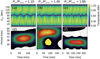 |
Fig. 9. Time-distance diagrams and wavelet analysis of the filament displacement with different quasi-periodic jets. Top row: time-distance diagrams of the temperature distributions in three cases when the driving period of the jets is 1.15Ppendu, 1.45Ppendu, and 1.85Ppendu, respectively. Bottom row: corresponding wavelet periodograms of the three cases, where the dashed black lines correspond to the significance of 95%, and the horizontal red line marks the pendulum period, Ppendu. |
For all the 20 cases, we performed a wavelet analysis of the evolution of the filament displacement to derive the “observed” oscillation period (Pobs). Its variation with the jet period Pobs is shown in Fig. 10, where both parameters are normalized by the pendulum period Ppendu. We found that Pobs indeed deviates from the intrinsic period of the pendulum model (Ppendu) when the filament is driven by periodic jets, and the deviation depends on the driving period of the jet, Pjet. As Pjet increases from Ppendu to 2Ppendu, the “observed” oscillation period (Pobs) first increases to more than 1.4Ppendu, then drastically drops to 0.9Ppendu, and then gradually increases back to Ppendu. Excluding the nonperiodic cases when Pjet is ∼1.5Ppendu, whose data points are color-coded in blue, all other cases (red data points) display quasi-period oscillations. We fit the red data points with the following formula:
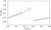 |
Fig. 10. Dependence of the observed period (Pobs) on the jet period Pjet in our parameter survey, where both quantities are normalized by Ppendu. The dashed blue line marks the intrinsic period determined by the pendulum model. |
With the least-squares method, the fitted parameters are a = −0.20, b = 1.20, c = 0.36, and d = 0.28. In real observations, the pendulum period Ppendu is an unknown. Therefore, we rewrite Eq. (7) in the following way:

With this formula, we can easily determine the pendulum period Ppendu (hence the curvature radius) of the magnetic dips once we have measured the decayless oscillation period (Pobs) and the driving period of jets Pjet.
In the 2014 July 5 event, the observed period of the filament decayless oscillation is Pobs ∼ 36.4 min, and the driving period of the jets is Pjet ∼ 68.9 ± 1.0 min. According to our Eq. (8), the pendulum oscillation period Ppendu should be 40.2 min, which corresponds to a curvature radius of 40.2 Mm. As a test, we performed another hydrodynamic simulation, with the parameters in Eq. (6) being l = 109.5 Mm and D = 20.2 Mm in order to match the curvature radius of R = 40.2 Mm. With the quasi-periodic jets impinging the filament, the filament starts to oscillate without decay. We found that the period of the decayless oscillations is 36.14 ± 0.62 min, which is almost the same as in observations.
We also note that although the fitted period of the decayless oscillations is not the intrinsic period of the pendulum model, the initial stage of the oscillation before the second jet hits the filament should be identical to the single-pulse case and hence should possess the pendulum period. Therefore, rather than fitting the whole evolution in Fig. 4, we fit the oscillation during the interval of 18:30–19:40 UT, and it is revealed that the fitted period is 40.0 ± 0.24 min, which is very close to the derived pendulum period from Eq. (8).
6. Summary
We used SDO/AIA and KSO Hα data to analyze the decayless longitudinal oscillations of the filament in active region AR12104 on 2014 July 5. The main results are summarized as follows:
-
The observations reveal that quasi-periodic homologous jets drive the large-amplitude decayless longitudinal oscillation of the filament before eruption. Our 1D hydrodynamic numerical simulations verified the causal relationship.
-
The decayless filament oscillations were followed by the filament eruption and a CME. All the observational features can be fit into the big picture of the CME triggering process described in Chen & Shibata (2000) and Chen et al. (2008): Interchange magnetic reconnection between the magnetic field of the filament system and the ambient results in two consequences: On the one hand, quasi-periodic jets are produced, which hit the filament, leading to decayless longitudinal oscillations. On the other hand, the post-reconnection large-scale field has a concave-upward kink, whose Lorentz force pulls the filament system to rise, triggering the onset of filament eruption. The ensuing magnetic reconnection below the filament makes the final eruption as described by the standard CME/flare model. Our data analysis and simulations validated the physical ground of the decayless filament oscillations as a precursor of CMEs.
-
When driven by quasi-periodic jets or other perturbations, the period of the filament longitudinal oscillations, Pobs, deviates from the intrinsic period of the pendulum model (Ppendu) up to 40% depending on the driving period of the jets, Pjet. One cannot use the pendulum model to derive the curvature radius directly. With a parameter survey, we propose an empirical formula to relate Pobs and Pjet to Ppendu (i.e., Eq. (8)). Alternatively, if we fit the oscillations in the initial stage before the second jet hits the filament, the fitted period is also the pendulum period, which can be used to derive the curvature radius of the magnetic dip.
It is noted that the filament plasma in our simulations was considered to be fully ionized for simplicity. In real situations the temperature of the filament plasma is ∼7000 K, where partial ionization and optically thick radiation begin to take effect for internal waves propagating inside the filament (Ballester et al. 2018, 2020, 2021). For the global pendulum mode oscillations studied in this paper, these internal waves are not directly involved. Still, if we were to consider partial ionization and optically thick radiation, they would increase the density of the filament thread, which might prolong the decay time for any episode of filament longitudinal oscillations. This effect will be studied in future papers.
Movie
Movie 1 associated with Fig. 2 (anim1) Access here
Acknowledgments
The authors thank the anonymous referee for constructive suggestions, and SDO and GONG teams for the open data policy. The research is funded by the National Key Research and Development Program of China (2020YFC2201200), NSFC (11961131002, 11773079, and 11533005), and the Strategic Priority Research Program on Space Science, CAS (XDA15052200, XDA15320301).
References
- Arregui, I., Oliver, R., & Ballester, J. L. 2018, Liv. Rev. Sol. Phys., 15, 3 [Google Scholar]
- Aulanier, G., & Schmieder, B. 2002, A&A, 386, 1106 [NASA ADS] [CrossRef] [EDP Sciences] [Google Scholar]
- Awasthi, A. K., Liu, R., & Wang, Y. 2019, ApJ, 872, 109 [NASA ADS] [CrossRef] [Google Scholar]
- Ballester, J. L., Carbonell, M., Soler, R., & Terradas, J. 2018, A&A, 609, A6 [NASA ADS] [CrossRef] [EDP Sciences] [Google Scholar]
- Ballester, J. L., Soler, R., Terradas, J., & Carbonell, M. 2020, A&A, 641, A48 [NASA ADS] [CrossRef] [EDP Sciences] [Google Scholar]
- Ballester, J. L., Soler, R., Carbonell, M., & Terradas, J. 2021, A&A, 656, A159 [NASA ADS] [CrossRef] [EDP Sciences] [Google Scholar]
- Berger, T. E., Slater, G., Hurlburt, N., et al. 2010, ApJ, 716, 1288 [Google Scholar]
- Chen, P. F., & Shibata, K. 2000, ApJ, 545, 524 [Google Scholar]
- Chen, P. F., Innes, D. E., & Solanki, S. K. 2008, A&A, 484, 487 [NASA ADS] [CrossRef] [EDP Sciences] [Google Scholar]
- Chen, H.-D., Zhang, J., & Ma, S.-L. 2012, Res. Astron. Astrophys., 12, 573 [Google Scholar]
- Chen, P. F., Harra, L. K., & Fang, C. 2014, ApJ, 784, 50 [NASA ADS] [CrossRef] [Google Scholar]
- Chen, J., Su, J., Yin, Z., et al. 2015, ApJ, 815, 71 [NASA ADS] [CrossRef] [Google Scholar]
- Chen, H., Zhang, J., Ma, S., Yan, X., & Xue, J. 2017, ApJ, 841, L13 [NASA ADS] [CrossRef] [Google Scholar]
- Chen, P.-F., Xu, A.-A., & Ding, M.-D. 2020, Res. Astron. Astrophys., 20, 166 [Google Scholar]
- Chen, J., Su, Y., Liu, R., et al. 2021, ApJ, 923, 142 [NASA ADS] [CrossRef] [Google Scholar]
- Cheung, M. C. M., De Pontieu, B., Tarbell, T. D., et al. 2015, ApJ, 801, 83 [Google Scholar]
- Dai, Y., Ding, M. D., Chen, P. F., & Zhang, J. 2012, ApJ, 759, 55 [NASA ADS] [CrossRef] [Google Scholar]
- Dai, J., Zhang, Q., Zhang, Y., et al. 2021, ApJ, 923, 74 [NASA ADS] [CrossRef] [Google Scholar]
- Duchlev, P., Koleva, K., Dechev, M., et al. 2010, BlgAJ, 14, 89 [NASA ADS] [Google Scholar]
- Gibson, S. E. 2018, Liv. Rev. Sol. Phys., 15, 7 [Google Scholar]
- Gosain, S., Schmieder, B., Venkatakrishnan, P., Chandra, R., & Artzner, G. 2009, Sol. Phys., 259, 13 [NASA ADS] [CrossRef] [Google Scholar]
- Guo, Y., Schmieder, B., Démoulin, P., et al. 2010, ApJ, 714, 343 [Google Scholar]
- Guo, Y., Xia, C., & Keppens, R. 2016a, ApJ, 828, 83 [NASA ADS] [CrossRef] [Google Scholar]
- Guo, Y., Xia, C., Keppens, R., & Valori, G. 2016b, ApJ, 828, 82 [NASA ADS] [CrossRef] [Google Scholar]
- Guo, Y., Xu, Y., Ding, M. D., et al. 2019, ApJ, 884, L1 [NASA ADS] [CrossRef] [Google Scholar]
- Guo, J. H., Ni, Y. W., Qiu, Y., et al. 2021, ApJ, 917, 81 [NASA ADS] [CrossRef] [Google Scholar]
- Hershaw, J., Foullon, C., Nakariakov, V. M., & Verwichte, E. 2011, A&A, 531, A53 [NASA ADS] [CrossRef] [EDP Sciences] [Google Scholar]
- Jing, J., Lee, J., Spirock, T. J., et al. 2003, ApJ, 584, L103 [NASA ADS] [CrossRef] [Google Scholar]
- Karpen, J. T., Antiochos, S. K., Hohensee, M., Klimchuk, J. A., & MacNeice, P. J. 2001, ApJ, 553, L85 [Google Scholar]
- Karpen, J. T., Antiochos, S. K., & Klimchuk, J. A. 2006, ApJ, 637, 531 [Google Scholar]
- Keppens, R., Meliani, Z., van Marle, A. J., et al. 2012, J. Comput. Phys., 231, 718 [Google Scholar]
- Kippenhahn, R., & Schlüter, A. 1957, ZAp, 43, 36 [NASA ADS] [Google Scholar]
- Kuperus, M., & Raadu, M. A. 1974, A&A, 31, 189 [NASA ADS] [Google Scholar]
- Kusano, K., Bamba, Y., Yamamoto, T. T., et al. 2012, ApJ, 760, 31 [NASA ADS] [CrossRef] [Google Scholar]
- Labrosse, N., Heinzel, P., Vial, J. C., et al. 2010, Space Sci. Rev., 151, 243 [Google Scholar]
- Lemen, J. R., Title, A. M., Akin, D. J., et al. 2012, Sol. Phys., 275, 17 [Google Scholar]
- Li, T., & Zhang, J. 2012, ApJ, 760, L10 [NASA ADS] [CrossRef] [Google Scholar]
- Liu, R., Kliem, B., Török, T., et al. 2012, ApJ, 756, 59 [Google Scholar]
- Luna, M., & Karpen, J. 2012, ApJ, 750, L1 [NASA ADS] [CrossRef] [Google Scholar]
- Luna, M., & Moreno-Insertis, F. 2021, ApJ, 912, 75 [NASA ADS] [CrossRef] [Google Scholar]
- Luna, M., Knizhnik, K., Muglach, K., et al. 2014, ApJ, 785, 79 [NASA ADS] [CrossRef] [Google Scholar]
- Luna, M., Karpen, J., Ballester, J. L., et al. 2018, ApJS, 236, 35 [NASA ADS] [CrossRef] [Google Scholar]
- Mackay, D. H., Karpen, J. T., Ballester, J. L., Schmieder, B., & Aulanier, G. 2010, Space Sci. Rev., 151, 333 [Google Scholar]
- Martin, S. F. 1990, in Solar Photosphere: Structure, Convection, and Magnetic Fields, ed. J. O. Stenflo, 138, 129 [NASA ADS] [CrossRef] [Google Scholar]
- Mashnich, G. P., & Bashkirtsev, V. S. 2016, Astron. Rep., 60, 287 [NASA ADS] [CrossRef] [Google Scholar]
- Mashnich, G. P., & Kiselev, A. V. 2019, Astron. Rep., 63, 608 [NASA ADS] [CrossRef] [Google Scholar]
- Mazumder, R., Pant, V., Luna, M., & Banerjee, D. 2020, A&A, 633, A12 [NASA ADS] [CrossRef] [EDP Sciences] [Google Scholar]
- Paraschiv, A. R., Donea, A., & Leka, K. D. 2020, ApJ, 891, 149 [NASA ADS] [CrossRef] [Google Scholar]
- Parenti, S. 2014, Liv. Rev. Sol. Phys., 11, 1 [Google Scholar]
- Scherrer, P. H., Schou, J., Bush, R. I., et al. 2012, Sol. Phys., 275, 207 [Google Scholar]
- Schmieder, B., Chandra, R., Berlicki, A., & Mein, P. 2010, A&A, 514, A68 [CrossRef] [EDP Sciences] [Google Scholar]
- Schmieder, B., Tian, H., Kucera, T., et al. 2014, A&A, 569, A85 [NASA ADS] [CrossRef] [EDP Sciences] [Google Scholar]
- Sharma, S. 2017, ARA&A, 55, 213 [Google Scholar]
- Shen, Y., Liu, Y. D., Chen, P. F., & Ichimoto, K. 2014a, ApJ, 795, 130 [Google Scholar]
- Shen, Y., Ichimoto, K., Ishii, T. T., et al. 2014b, ApJ, 786, 151 [NASA ADS] [CrossRef] [Google Scholar]
- Shen, Y., Liu, Y., Liu, Y. D., et al. 2015, ApJ, 814, L17 [Google Scholar]
- Shen, Y., Liu, Y. D., Su, J., Qu, Z., & Tian, Z. 2017, ApJ, 851, 67 [NASA ADS] [CrossRef] [Google Scholar]
- Shibata, K., Ishido, Y., Acton, L. W., et al. 1992, PASJ, 44, L173 [Google Scholar]
- Shibata, K., Nitta, N., Strong, K. T., et al. 1994, ApJ, 431, L51 [Google Scholar]
- Steinegger, M., Denker, C., Goode, P. R., et al. 2000, in The Solar Cycle and Terrestrial Climate, Solar and Space weather, ed. A. Wilson, ESA Spec. Pub., 463, 617 [NASA ADS] [Google Scholar]
- Terradas, J., Soler, R., Oliver, R., & Ballester, J. L. 2015, ApJ, 802, L28 [NASA ADS] [CrossRef] [Google Scholar]
- Tian, H., DeLuca, E. E., Cranmer, S. R., et al. 2014, Science, 346, 1255711 [Google Scholar]
- Titov, V. S., Downs, C., Mikić, Z., et al. 2018, ApJ, 852, L21 [NASA ADS] [CrossRef] [Google Scholar]
- Török, T., Downs, C., Linker, J. A., et al. 2018, ApJ, 856, 75 [Google Scholar]
- van Ballegooijen, A. A. 2004, ApJ, 612, 519 [NASA ADS] [CrossRef] [Google Scholar]
- van Ballegooijen, A. A., Priest, E. R., & Mackay, D. H. 2000, ApJ, 539, 983 [NASA ADS] [CrossRef] [Google Scholar]
- Vial, J.-C., & Engvold, O. 2015, Solar Prominences, 415 (Switzerland: Springer International Publishing) [Google Scholar]
- Wang, Y. M. 1999, ApJ, 520, L71 [Google Scholar]
- Xia, C., Chen, P. F., Keppens, R., & van Marle, A. J. 2011, ApJ, 737, 27 [NASA ADS] [CrossRef] [Google Scholar]
- Xia, C., Teunissen, J., El Mellah, I., Chané, E., & Keppens, R. 2018, ApJS, 234, 30 [Google Scholar]
- Yan, X. L., Xue, Z. K., Pan, G. M., et al. 2015, ApJS, 219, 17 [Google Scholar]
- Yang, L.-H., Jiang, Y.-C., Yang, J.-Y., et al. 2011, Res. Astron. Astrophys., 11, 1229 [CrossRef] [Google Scholar]
- Yang, L., Yan, X., Li, T., Xue, Z., & Xiang, Y. 2017, ApJ, 838, 131 [NASA ADS] [CrossRef] [Google Scholar]
- Zhang, Q. M. 2020, A&A, 642, A159 [NASA ADS] [CrossRef] [EDP Sciences] [Google Scholar]
- Zhang, Q. M., & Ji, H. S. 2018, ApJ, 860, 113 [NASA ADS] [CrossRef] [Google Scholar]
- Zhang, Q. M., Chen, P. F., Xia, C., & Keppens, R. 2012, A&A, 542, A52 [NASA ADS] [CrossRef] [EDP Sciences] [Google Scholar]
- Zhang, Q. M., Chen, P. F., Xia, C., Keppens, R., & Ji, H. S. 2013, A&A, 554, A124 [NASA ADS] [CrossRef] [EDP Sciences] [Google Scholar]
- Zhang, Q. M., Li, D., & Ning, Z. J. 2017, ApJ, 851, 47 [NASA ADS] [CrossRef] [Google Scholar]
- Zhang, Q. M., Guo, J. H., Tam, K. V., & Xu, A. A. 2020, A&A, 635, A132 [NASA ADS] [CrossRef] [EDP Sciences] [Google Scholar]
- Zhou, Y.-H., Zhang, L.-Y., Ouyang, Y., Chen, P. F., & Fang, C. 2017, ApJ, 839, 9 [NASA ADS] [CrossRef] [Google Scholar]
All Tables
Parameters of simulated filament oscillations in the control case and the multipulse case.
All Figures
|
Fig. 1. Multiwavelength imaging observations on the AR filament. Panel a: corresponding Hα image of the filament provided by the Kanzelhöhe Observatory at 13:10:46 UT, where the red and blue contour lines represent different levels of magnetic field strength ranging from −50 G to 50 G. The arrow indicates a right-bearing barb of the filament. Panel b: SDO/AIA 304 Å image observed at 13:10:43 UT. Panel c: SDO/AIA 171 Å image observed at 23:19:36 UT. The arrows mark left-skewed flare loops formed after the filament eruption. |
| In the text | |
|
Fig. 2. Temporal evolution of the AR filament in AIA 171 Å from 18:35 UT to 22:20 UT. In panel a, a slice is chosen in order to plot the time-distance diagram in Fig. 3. The black arrow in panel b marks dark features accompanying the jets. The animation of this figure is available online. |
| In the text | |
|
Fig. 3. Time-distance diagram of the AIA 171 Å intensity along the slice marked in Fig. 2a. The distance increases from west to east, therefore the dark ridge with a strong slope around 22:40 UT means that the filament was erupting toward the west. The figure indicates decayless filament oscillations associated with quasi-periodic jets. |
| In the text | |
|
Fig. 4. Panel a: close-up view of Fig. 3 around the filament, highlighting the filament oscillations. Panel b: evolution of the filament centroid (red error bars) and the fitted curve (black line). |
| In the text | |
|
Fig. 5. Temporal evolution and nonlinear force-free field extrapolation model of the AR filament. Panels a–d: four snapshots of the SDO/HMI magnetogram around the filament channel, where white and black means positive and negative polarity, and the red squares correspond to the site of the jet source. The filament spine is represented by the dashed cyan lines. Panel e: coronal magnetic field reconstructed using the RBSL flux rope and magneto-frictional model. The green field lines represent the flux rope and the yellow lines indicate that the overlying magnetic field contains a fan-spine structure. The red cube corresponds to the red squares in the top four panels, where magnetic reconnection probably occurred. |
| In the text | |
|
Fig. 6. Geometry of the flux tube in our simulations, where the central part is a helix described by Eq. (5). The natural coordinate is along the tube starting from the left footpoint. |
| In the text | |
|
Fig. 7. Top row: time-distance diagrams of the temperature distribution along the magnetic flux tube in the control case (left) and in the multipulse case (right). Bottom row: temporal evolution of the displacement of the filament thread center in the control case (left) and in the multipulse case (right), where the dashed black lines correspond to the simulation results, and the solid red lines correspond to the fitting curves. |
| In the text | |
|
Fig. 8. Schematic sketch of the magnetic reconnection process, which triggers both repetitive jets and the onset of the filament eruption. The green line AB represents the magnetic field supporting the filament, and the cyan line CD represents the neighboring strongly sheared field line. The interchange reconnection between lines AB and CD leads to jets and to the expansion of the post-reconnection field line AD. |
| In the text | |
|
Fig. 9. Time-distance diagrams and wavelet analysis of the filament displacement with different quasi-periodic jets. Top row: time-distance diagrams of the temperature distributions in three cases when the driving period of the jets is 1.15Ppendu, 1.45Ppendu, and 1.85Ppendu, respectively. Bottom row: corresponding wavelet periodograms of the three cases, where the dashed black lines correspond to the significance of 95%, and the horizontal red line marks the pendulum period, Ppendu. |
| In the text | |
|
Fig. 10. Dependence of the observed period (Pobs) on the jet period Pjet in our parameter survey, where both quantities are normalized by Ppendu. The dashed blue line marks the intrinsic period determined by the pendulum model. |
| In the text | |
Current usage metrics show cumulative count of Article Views (full-text article views including HTML views, PDF and ePub downloads, according to the available data) and Abstracts Views on Vision4Press platform.
Data correspond to usage on the plateform after 2015. The current usage metrics is available 48-96 hours after online publication and is updated daily on week days.
Initial download of the metrics may take a while.