| Issue |
A&A
Volume 663, July 2022
|
|
|---|---|---|
| Article Number | A48 | |
| Number of page(s) | 19 | |
| Section | Planets and planetary systems | |
| DOI | https://doi.org/10.1051/0004-6361/202142915 | |
| Published online | 14 July 2022 | |
The CARMENES search for exoplanets around M dwarfs
Two Saturn-mass planets orbiting active stars★
1
Landessternwarte, Zentrum für Astronomie der Universität Heidelberg,
Königstuhl 12,
69117
Heidelberg, Germany
e-mail: This email address is being protected from spambots. You need JavaScript enabled to view it.
2
Hamburger Sternwarte,
Gojenbergsweg 112,
21029
Hamburg, Germany
3
Homer L. Dodge Department of Physics and Astronomy, University of Oklahoma,
440 West Brooks Street,
Norman, OK
73019, USA
4
Max-Planck-Institut für Astronomie,
Königstuhl 17,
69117
Heidelberg, Germany
5
Department of Astronomy, Sofia University “St Kliment Ohridski”,
5 James Bourchier Blvd,
1164
Sofia, Bulgaria
6
Instituto de Astrofísica de Andalucía (CSIC),
Glorieta de la Astronomía s/n,
18008
Granada, Spain
7
Centro de Astrobiología (CSIC-INTA), ESAC,
Camino Bajo del Castillo s/n,
28692
Villanueva de la Cañada, Madrid, Spain
8
Institut für Astrophysik, Georg-August-Universität Göttingen,
Friedrich-Hund-Platz 1,
37077
Göttingen, Germany
9
Institut de Ciències de l’Espai (ICE, CSIC),
Campus UAB, c/ de Can Magrans s/n,
08193
Bellaterra, Barcelona, Spain
10
Institut d’Estudis Espacials de Catalunya (IEEC),
08034
Barcelona, Spain
11
Centro Astronómico Hispano-Alemán (MPG-CSIC), Observatorio Astronómico de Calar Alto,
Sierra de los Filabres,
04550
Gérgal, Almería, Spain
12
Instituto de Astrofísica de Canarias,
c/ Vía Láctea s/n,
38205
La Laguna, Tenerife, Spain
13
Departamento de Astrofísica, Universidad de La Laguna,
38206
Tenerife, Spain
14
Thüringer Landessternwarte Tautenburg,
Sternwarte 5,
07778
Tautenburg, Germany
15
School of Physics & Astronomy, University of Birmingham, Edgbaston,
Birmingham
B15 2TT, UK
16
Departamento de Física de la Tierra y Astrofísica & IPARCOS-UCM (Instituto de Física de Partículas y del Cosmos de la UCM), Facultad de Ciencias Físicas, Universidad Complutense de Madrid,
28040
Madrid, Spain
17
Department of Physics, University of Warwick,
Coventry
CV4 7AL, UK
18
Department of Physics, Ariel University,
Ariel
40700, Israel
19
Centro de Astrobiología (CSIC-INTA), Campus INTA,
Carretera de Ajalvir km 4,
28850
Torrejón de Ardoz, Madrid, Spain
Received:
10
December
2021
Accepted:
15
March
2022
Abstract
The CARMENES radial-velocity survey is currently searching for planets in a sample of 387 M dwarfs. Here we report on two Saturn-mass planets orbiting TYC 2187-512-1 (M* = 0.50 M⊙) and TZ Ari (M* = 0.15 M⊙), respectively. We obtained supplementary photometric time series, which we use along with spectroscopic information to determine the rotation periods of the two stars. In both cases, the radial velocities also show strong modulations at the respective rotation period. We thus modeled the radial velocities as a Keplerian orbit plus a Gaussian process representing the stellar variability. TYC 2187-512-1 is found to harbor a planet with a minimum mass of 0.33 MJup in a near-circular 692-day orbit. The companion of TZ Ari has a minimum mass of 0.21 MJup, orbital period of 771 d, and orbital eccentricity of 0.46. We provide an overview of all known giant planets in the CARMENES sample, from which we infer an occurrence rate of giant planets orbiting M dwarfs with periods up to 2 yr in the range between 2 and 6%. TZ Ari b is only the second giant planet discovered orbiting a host with mass less than 0.3 M⊙. These objects occupy an extreme location in the planet mass versus host mass plane. It is difficult to explain their formation in core-accretion scenarios, so they may possibly have been formed through a disk fragmentation process.
Key words: planets and satellites: detection / planets and satellites: formation / stars: individual: TZ Ari / stars: individual: TYC 2187-512-1 / stars: low-mass / techniques: radial velocities
The CARMENES radial-velocity data are only available at the CDS via anonymous ftp to cdsarc.u-strasbg.fr (130.79.128.5) or via http://cdsarc.u-strasbg.fr/viz-bin/cat/J/A+A/663/A48
© ESO 2022
1 Introduction
The occurrence rate of giant planets depends on the properties of their host stars. This can be understood in the context of their formation and early migration in the circumstellar disk. As a general trend, the dust masses in protoplanetary disks increase with the mass of their host (Manara et al. 2018). Likewise, the number of gas giants in orbits with periods up to a few years increases with stellar mass (Johnson et al. 2010a), with an apparent maximum near 2 M⊙ and a sharp decline towards even higher masses (Reffert et al. 2015). Surveys for planets orbiting M dwarfs play an important role in this context, as this spectral type spans nearly an order of magnitude in mass, from the hydrogen burning limit at 0.07 M⊙ to about 0.6 M⊙. While the first planet found around an M dwarf, GJ 876 b, is surprisingly massive with m = 2.1 MJup (Marcy et al. 1998; Delfosse et al. 1998; Trifonov et al. 2018), gas giants orbiting M dwarfs are actually quite rare (Bonfils et al. 2013; Sabotta et al. 2021). In a similar vein, a trend of fewer large planets with radii of R ≳ 1.4 R⊕ is found towards decreasing stellar temperatures (Dressing & Charbonneau 2013).
Giant planets orbiting low-mass stars contain important information about planet formation processes, as they challenge the core accretion paradigm and, specifically, pebble accretion as the dominant mechanism of core growth (Morales et al. 2019). Here, we report on the discovery of two Saturn-mass planets from the CARMENES survey, which is currently carrying out precise radial-velocity (RV) observations of a sample of 387 M dwarfs (for a recent overview, see Quirrenbach et al. 2020). As both host stars TYC 2187-512-1 and TZ Ari also show clear RV variations at the stellar rotation period, we modeled these as Gaussian processes (GPs) alongside the Keplerian signals.
Section 2 contains the fundamental parameters and other pertinent information about the two target stars. In Sect. 3, we describe supplementary photometry carried out at several observatories. The CARMENES observations of both stars, and RVs of TZ Ari gathered from the HARPS and HIRES archives, are presented in Sect. 4. Photometric and spectroscopic information is combined in Sect. 5 to determine the stellar rotation periods. In Sect. 6, we introduce our GP model, apply it to the RV time series, and determine the planetary parameters. We discuss our results in Sect. 7 and conclude with a summary in Sect. 8.
2 Target stars
Table 1 provides a summary of the stellar properties of both stars. In this section, we provide a brief description of how they were derived.
2.1 TYC 2187-512-1
The star TYC 2187-512-1 (Karmn J21221+2291) is an early M dwarf with spectral type M1.0V (Lépine et al. 2013). We adopted the distance of 15.485 ± 0.005 pc from Gaia EDR3 (π = 64.580 ± 0.021 mas, Gaia Collaboration 2021). The photo-spheric parameters effective temperature, Teff, surface gravity, log g, and metallicity, [Fe/H], were determined by Passegger et al. (2019). These authors used updated PHOENIX models with the latest atomic and molecular line lists, updated Solar abundances (Caffau et al. 2011), and a new equation of state (Meyer 2017), and fitted them to high-resolution CARMENES spectra in the visible and near-infrared wavelength ranges. During this process, a rotational velocity of v sin i* = 2 km s–1 was assumed, which was reported as the upper limit for this star by Reiners et al. (2018). A recent analysis by Marfil et al. (2021) with the SteParSyn code (Tabernero et al. 2022) yielded systematically lower values of [Fe/H]; the difference of about 0.2 dex is indicative of persistent difficulties in determining accurate parameters for M dwarfs. The bolometric luminosity, L, was taken from Schweitzer et al. (2019). The spectral energy distribution was integrated from a number of apparent magnitudes in broad band passes over the whole spectral range from the blue optical to the mid-infrared, as described by Cifuentes et al. (2020). Together with the Gaia distance, the luminosity, L, can be derived. The stellar radius was calculated from Teff and L via the Stefan-Boltzmann law. With this, we derived the stellar mass from the mass-radius relation of Schweitzer et al. (2019). The pseudo-equivalent width pEW(Hα) is +0.4 ± 0.1 Å (Jeffers et al. 2018; Lépine et al. 2013; Gaidos et al. 2014)2. A slightly different quantity, pEW′(Hα), is given by Schöfer et al. (2019). It is defined by subtracting the spectrum of an inactive star before computing the pEW, thus isolating the emission component of the line. The value for TYC 2187-512-1 is –0.032 ± 0.006 Å. From our CARMENES spectra, we find the star to be moderately active, with clear signals in the activity indicators, but no Hα emission in the individual spectra.
2.2 TZ Ari
Different spectral types have been given in the literature for the M dwarf TZ Ari (Karmn J02002+130, Gl83.1). Lépine et al. (2013) claimed the star to be an M5.0V, whereas Alonso-Floriano et al. (2015) stated it was an M3.5: V. Considering Teff, measured by Passegger et al. (2019) (spectroscopic, 3154 ± 54 K) and Houdebine et al. (2019) (photometric, 3158 ± 23 K), a spectral type of M5.0 V seems to be a more accurate assumption. TZ Ari is very close to the Sun, with a distance of only 4.470 ± 0.001 pc (π = 223.73 ± 0.07 mas, Gaia Collaboration 2021). The bolometric luminosity as well as the stellar radius and mass were calculated in the same way as for TYC 2187-512-1. The parameters Teff, log g, and [Fe/H] were taken from Passegger et al. (2019). Regarding the projected rotational velocity, Reiners et al. (2018) measured an upper limit of 2 km s–1. There is no rotational period in the literature for this star (but see Sect. 5); from υ sin i* and the stellar radius we can estimate a lower limit of Prot/ sin i* > 4.15 d. This M dwarf is a flare star (Kunkel 1968; Rodríguez Martínez et al. 2020), hence, its variable star designation. It shows significant Hα emission with pEW(Hα) measurements yielding –2.056 ± 0.012 Å (Jeffers et al. 2018) or –1.981 ± 0.030 Å (Newton et al. 2017) and pEW′(Hα) = –1.906 ± 0.025 Å (Schöfer et al. 2019).
2.3 Kinematics and ages
Kinematically, both stars are members of the thin disk, without any obvious membership in a moving group or association (Cortés-Contreras et al. 2020). With a rotation period of 40 d (see Sect. 5), TYC 2187-512-1 is most likely older than 2.5 Gyr. TZ Ari is a much faster rotator, but a comparison with M dwarfs of known ages (Popinchalk et al. 2021) indicates that its age is no younger than that of the Hyades, 750 Myr.
We also queried the Gaia EDR3 database for wide co-moving companions within a search radius of 2°, but did not find any objects with a matching parallax.
3 Photometry
3.1 SuperWASP
The Super-Wide Angle Search for Planets (SuperWASP) Survey (Pollacco et al. 2006) comprises two robotic eight-camera telescope arrays stationed in La Palma, Spain and in Sutherland, South Africa. The cameras each have a CCD with a field size of ~60 deg2, giving a plate scale of 13.″7 pixel–1. They are fitted with broadband filters spanning 400 to 700 nm. In operation since 2004, these systems monitor the entire sky at high cadence and deliver good quality photometry (i.e., characteristic precision ≲1 %) for objects with V ≲ 11.5 mag.
SuperWASP collected data on TYC 2187-512-1 and TZ Ari from 2004 to 2010, and from 2008 to 2011, respectively. The light curves were extracted and de-trended following the methods of Tamuz et al. (2005), which were designed to remove instrumental systematics while preserving astrophysical signals.
Stellar parameters of TYC 2187-512-1 and TZ Ari.
3.2 Las Cumbres Observatory (LCOGT)
We obtained V and I′-band images of TYC 2187-512-1 using the 40 cm telescopes of LCOGT (Brown et al. 2013) at the Haleakalā (Maui) and Teide (Canary Islands) sites at 63 different epochs between June 28 and September 4, 2018. We acquired 50 individual exposures of 10 s in the V-band and 5 s in the I′-band per visit. The telescopes are equipped with a 3k × 2k SBIG CCD camera with a pixel scale of 0.″571 providing a field of view of 29.′2 × 19.′5. The weather at the observatories was clear in general; the average seeing varied from 1.″3 to 3.″1. The raw data were processed using the BANZAI pipeline (McCully et al. 2018), which includes bad pixel, bias, dark, and flat field corrections for each individual night. Aperture photometry was obtained for TYC 2187-512-1 and several reference stars in the field using apertures of 11 pixels (6.″3). These apertures minimize the dispersion of the relative differential photometry between the target and reference stars.
TZ Ari was observed in the I′ band from the Siding Spring, Cerro Tololo, McDonald, and South African Astronomical Observatory sites of the LCOGT. A total of 538 photometric measurements were taken between September 29, 2019 and February 17, 2020. The data were reduced in the same way as those of TYC 2187-512-1.
3.3 Sierra Nevada Observatory (OSN)
Photometric observations of TYC 2187-512-1 and TZ Ari were also collected at Observatorio de Sierra Nevada (OSN), Granada, Spain, using the T90 and T150 telescopes. T90 is a 90 cm Ritchey-Chrétien telescope equipped with a VersArray 2k × 2k pixel CCD camera, providing a field of view of 13.′2 × 13.′2. The camera is based on a back-illuminated Marconi-EEV CCD42-4 with optimized response in the ultraviolet (Rodr guez et al. 2010). Observations of TYC 2187-512-1 were collected in Johnson V and R filters on 50 nights during the period between May and August 2018. Each CCD frame was corrected in a standard way for bias and flatfielding. All CCD measurements were obtained by the method of synthetic aperture photometry. Different aperture sizes were tested in order to choose the best one for our observations. A number of nearby and relatively bright stars within the frames were selected as reference stars. The data, in each filter, are presented as magnitude differences, normalized to zero. Outliers due to bad weather conditions or high airmass have been removed.
T150 is a 150 cm Ritchey-Chrétien telescope equipped with a back-illuminated Andor Ikon-L DZ936N-BEX2-DD 2k × 2k CCD camera, with a resulting field of view of 7.′92 × 7.′92. The camera is cooled thermo-electrically to −100 °C for negligible dark current. The observations of TZ Ari were collected in Johnson V and R filters on 42 nights during the period September 2019 to January 2020, and reduced in the same way as for T90.
3.4 Montsec Observatory (OdM)
Observations with the 80 cm Joan Oró telescope at Montsec Observatory (Sant Esteve de la Sarga, Catalonia) were conducted using its main imaging camera LAIA, a 4k × 4k back-illuminated CCD with a pixel scale of 0.″4 and a field of view of 30′, using a Johnson R filter. Several blocks of five images were obtained per night during the visibility periods of TZ Ari, resulting on 3115 measurements from February 2019 to March 2020. The images were calibrated with dark frames, bias, and flat fields, using the ICAT pipeline (Colome & Ribas 2006). Differential photometry was extracted with AstroImageJ (Collins et al. 2017), using the aperture size and the set of comparison stars that minimized the rms of the photometry.
4 Spectroscopy
4.1 CARMENES
TYC 2187-512-1 and TZ Ari are included in the CARMENES radial-velocity survey of M dwarfs (Quirrenbach et al. 2016; Reiners et al. 2018), which is currently being conducted with the 3.5 m telescope at the Calar Alto observatory (CAHA) in Almería, Spain. The CARMENES instrument was designed and optimized specifically for this survey. It consists of two cross-dispersed échelle spectrographs covering the wavelength regions 5200–9600 Å (VIS) and 9600–17 100 Å (NIR) with a spectral resolution of  and
and  , respectively (Quirrenbach et al. 2014, 2018).
We obtained 94 VIS and 96 NIR observations of TYC 2187-512-1, with exposure times ranging from 900 to 1800 s, depending on seeing and sky transparency. TZ Ari was observed 93 times with the VIS and 89 times with the NIR spectrograph, using similar exposure times. All the spectra were accompanied by simultaneous Fabry-Pérot spectra; the FP etalons were calibrated during daytime with Th-Ne, U-Ar, and U-Ne hollow-cathode lamps to establish an absolute wavelength scale.
All data were processed with the standard CARMENES pipelines (Caballero et al. 2016b). The data reduction pipeline caracal applies standard corrections for detector bias and dark current, traces the échelle orders, extracts the spectra, and provides the wavelength calibration. The resulting fully reduced visible-light and near-infrared spectra are then analyzed with a second pipeline, serval (Zechmeister et al. 2018). This process computes the RV of each observation by cross-correlating the corresponding spectrum with a reference template constructed from all observed spectra of the same star. In addition, serval provides a number of spectral line indices3, which can be useful diagnostic tools for stellar variability, as well as indicators of the differential line width (dLW) and of the wavelength-dependence of the RV (chromatic index, CRX; for details see Zechmeister et al. 2018). Further small corrections to the observed RVs are applied as described by Trifonov et al. (2018).
The CARMENES RVs of TYC 2187-512-1 and TZ Ari determined in this way are available from CDS. We note that for stars with spectral types of M1 V (TYC 2187-512-1) and even as late as M5 V (TZ Ari), the spectral information content in the VIS channel of CARMENES is much higher than in the NIR (Reiners et al. 2018). This leads to substantially smaller formal errors for the VIS data (independent of any calibration errors), as the VIS and NIR observations are executed simultaneously and thus with nearly identical integration times. Therefore, here we analyze mainly the VIS data, and we use the NIR data only to validate the planetary nature of TZ Ari b (see Sect. 6.3.3).
4.2 Archival data
To complement our CARMENES data, we searched publicly available databases for precise RV time series of our two targets. No additional data were found for TYC2187-512-1, but TZ Ari has been observed with HIRES/Keck and with HARPS.
The High Resolution Echelle Spectrograph (HIRES, Vogt et al. 1994), installed at the right Nasmyth focus of the Keck I telescope, has been used extensively for RV monitoring with the iodine cell method. RV time series of 1624 stars obtained with this instrument were published by Butler et al. (2017). We have used an improved version of these data (Tal-Or et al. 2019), which have been corrected for small nightly zero points and for a jump due to a CCD upgrade in 2004. This data set contains 54 observations of TZ Ari spread out over 13 yr, with typical formal precision of 3.5 m s–1. Butler et al. (2017) also tabulated the Ca II H&K S index and an Hα index, but the values of the S index scatter widely (which is no surprise given the very low flux of M stars in the Ca II H&K spectral region), and there are many invalid entries for the Hα index. We therefore did not use any activity indicators from HIRES.
The HARPS instrument (Mayor et al. 2003) at the European Southern Observatory’s 3.6m telescope on La Silla, Chile, has pioneered the use of highly stabilized vacuum spectrographs for precise RV measurements. Twenty-five observations of TZ Ari with a typical RV precision of 4 m s–1 were found in the ESO archive. Trifonov et al. (2020b) have re-processed the archival HARPS data with serval, yielding an improved RV precision for most stars. In the case of TZ Ari, however, we find the results from the original HARPS pipeline to be of superior quality; this is probably because the re-processing was not tuned for spectral types later than early M. We therefore used the HARPS RVs as retrieved from the ESO archive. In view of the relatively small number of HARPS data points, we did not attempt to extract time series of activity indicators from them.
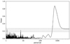 |
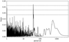
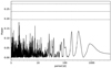
Fig. 1 GLS periodogram of the RV time series of TYC 2187-512-1 from CARMENES. The prominent peak at 696 d can be attributed to a planet. The marginally significant peak at 7.15 d and its alias at 1.15 d are due to the window function of the sampling. The insignificant but noticeable power near 40 d corresponds to the rotation period of the star. False-alarm probabilities of 0.1, 0.01, and 0.001 are shown as dashed horizontal lines. |
4.3 Periodograms
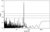
Figures 1 and 2 show generalized Lomb-Scargle (GLS, Zechmeister & Kürster 2009) periodograms of the RV time series of TYC2187-512-1 and TZ Ari, respectively. The periods apparent in these figures are analyzed in detail in the subsequent sections. Here, we give a brief overview. We attribute the most prominent peak in the TYC 2187-512-1 periodogram at 696 d to a planet, whereas the weaker peak at 7.15 d and its one-day alias at 1.15 d are due to the window function of the time series sampling. There is also some power near 40 d, which corresponds to the rotation period of the star, as corroborated by the photometric data and spectroscopic indicators. The most significant peak in the GLS diagram of TZ Ari at 781 d is also attributed to a planetary companion. The stellar rotation gives rise to the peak at 1.96 d. The other peaks in Fig. 2 are related to these two through harmonics and their aliases; they will thus disappear in the residuals after modeling the planetary and rotational signals (see Fig. 15).
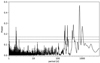 |
Fig. 2 GLS periodogram of the combined RV time series of TZ Ari from CARMENES, HIRES, and HARPS. The prominent peaks at 781 d and 1.96 d correspond to a planet and to the stellar rotation period, respectively. False-alarm probabilities of 0.1, 0.01, and 0.001 are shown as dashed horizontal lines. |
Rotation periods of TYC2187-512-1 and TZ Ari estimated from different data sets.
5 Rotation periods and activity
5.1 Rotation period of TYC2187-512-1
The photometric light curves of TYC 2187-512-1 from Super-WASP, LCOGT, and OSN all show a periodicity near 40 d (see Table 2), indicating that this is the rotation period of the star. A subset of the SuperWASP data was already analyzed by Díez Alonso et al. (2019), who arrived at a value of 41.0 ± 1.7 d. The CARMENES pipeline delivers several indicators that can also be used to determine rotation periods (Fuhrmeister et al. 2019; Lafarga et al. 2021); the most useful among these are the pEW of the Hα line, an index of the Ca II infrared triplet (IRT), the CRX, and the dLW. Three of these (Hα, IRT, and dLW) show the 40 d periodicity very clearly (see Appendix A for two examples), and there is also a strong peak near this value in the periodogram of the RVs. Taking into account the dispersion between these individual indicators, we conclude that the rotation period of TYC 2187-512-1 is 40 + 1 d.
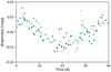 |
Fig. 3 Differential photometry of TYC 2187-512-1, phase-folded to P = 40.0203 d. Each data point represents measurements averaged over one night. SuperWASP data are shown as blue circles, and OSN R-band data are represented by green triangles. Within each of the two time series, the symbols change from light to dark with progressing time. See the text for more details. |
5.2 Activity of TYC 2187-512-1
A comparison between the time series of TYC 2187-512-1 taken from 2004 to 2010 with SuperWASP and the more recent observations, for instance, with OSN in 2018, reveals a striking persistence and consistency of the photometric variability of the star, both in amplitude and phase. A combined periodogram of the SuperWASP and OSN data shows multiple narrow peaks with almost identical amplitudes near 40 d, which are aliases of each other, resulting from the wide gap between the two data sets. We picked one of them at 40.0203 d and phase-folded the SuperWASP and OSN data to this period, without any attempt to account for the differences between the filters used by the two instruments. Nonetheless, the two light curves match almost perfectly (see Fig. 3), indicating that the photometric behavior of the star has remained remarkably stable for one and a half decades. A similar stable pattern was reported for the fully convective M4 dwarf V374 Peg (Vida et al. 2016). This is to be contrasted with LQ Hya, a BY Dra-type variable of spectral type K2 V, in which active areas on the stellar surface remain stable only on time scales less than a year (Lehtinen et al. 2012). Such observations provide valuable input for stellar dynamo models. A better understanding of the persistence of activity patterns is also important in the context of exoplanet detection, as stable RV modulations can easily be mistaken for the signature of a planet if the stellar rotation period is not known. Systematic studies of larger samples are therefore urgently needed, but the precision of current ground-based surveys such as ASAS is marginal for this type of work (Suárez Mascareño et al. 2016).
The Hα absorption line is slightly shallower in TYC 2187-512-1 than in an inactive reference star (Schöfer et al. 2019). This means that the line core is partially filled by an emission component, qualifying TYC 2187-512-1 as “Hα active”. Figure 4 shows the same photometric data as Fig. 3, in 20 equally spaced phase bins, along with the Hα line index as defined by Zechmeister et al. (2018) from the CARMENES spectra. From this plot it is evident that brightness and line index track each other very closely and consistently. Whenever the star is fainter (more positive magnitude), the line index is larger, namely, the core of the Hα line is more filled-in. This suggests that dark spotted patches on the stellar surface are accompanied by Hα emission regions.
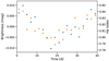 |
Fig. 4 Photometry and Hα index of TYC 2187-512-1, phase-folded to P = 40.0203 d and averaged into 20 equally spaced phase bins. The photometric data from SuperWASP and OSN (R-band) are shown in blue, and the Hα line index from CARMENES is shown in orange. |
5.3 Rotation period of TZ Ari
The R-band photometric variability amplitude of TZ Ari is only ~3 mmag, which makes it difficult to unambiguously identify its rotation period from ground-based monitoring data. Since TZ Ari will not be observed by TESS during cycles 1 through 4 (Sectors 1 through 55), we therefore start with the CARMENES spectroscopy. The RVs show a strong modulation with a period of 1.96 d and an amplitude that is not completely stable, but instead varying around a typical level of ~10 m s–1 (see also Figs. 12 and 13). These RV variations are chromatic, and thus cannot be caused by Doppler shifts due to an orbiting companion. Variations with the same periodicity are also observed in the Hα and Call IRT lines (see Table 2 and Appendix A), strengthening the conclusion that 1.96 d is the rotation period.
With this information in mind, the photometry can now be interpreted with confidence. The periodograms of the OSN R and V data both show a strong peak at 1.96 d, along with its slightly weaker daily alias at 2.03 d. The strongest peak for SuperWASP, at 131 d, can be attributed to instrumental effects, but again there are highly significant peaks at 1.96 d and 2.03 d. A peak at 1.96 d is also found for the Montsec time series, although it is not the highest in that periodogram. The LCOGT photometry is not precise enough to be useful for the determination of the rotation period of TZ Ari. Overall, the photometric variations thus fully confirm that the rotation period is 1.96 ± 0.02 d.
5.4 Activity of TZ Ari
The Hα line in TZ Ari is observed strongly in emission with temporally variable equivalent width, qualifying TZ Ari also as an Hα active star (Schöfer et al. 2019). White-light flares with amplitude up to ΔV = 0.87 were found in the light curve of TZ Ari from the ASAS-SN monitoring survey (Rodríguez Martínez et al. 2020). These findings are to be contrasted with the small rotational modulation of the stellar brightness. We can thus plausibly infer that chromospheric activity occurs rather uniformly over the stellar surface, or in regions with a uniform longitudinal distribution. However, the strong rotation-related RV variations point towards a significantly structured photosphere.
6 Modeling of the radial velocities and planet parameters
6.1 Gaussian process modeling
Stellar rotation induces quasi-periodic variations in the brightness, activity indicators, line shapes, and RV as spots, plage, and active regions rotate into and out of view (Dumusque et al. 2014). These variations can be used to determine the rotation period and to characterize various aspects of stellar activity, as discussed in the previous section. On the other hand, rotational modulation of the RVs may obscure the Keplerian signature of exoplanets, mimic spurious planets, or affect the planet parameters derived from models of the RV data. Therefore, any realistic comprehensive model of the RVs should be the sum of two components describing Keplerian orbits and stellar variability, respectively. The latter can be represented by a Gaussian process (e.g. Haywood et al. 2014), and the best-fit model is found by maximizing the likelihood, varying the Keplerian parameters and the hyper-parameters of the GP simultaneously. Several software packages are available to perform this task; we use the Exo-Striker (Trifonov 2019).
An important aspect of the RV modeling is the choice of the kernel function describing the noise covariance in the GP model. A physically well-motivated choice is the quasi-periodic kernel (e.g., Rajpaul et al. 2015):
![Mathematical equation: $k\left( \tau \right) = a\,\exp \left[ { - {{{\tau ^2}} \over {2{l^2}}} - {\rm{\Gamma }}\,{{\sin }^2}\left( {{{\pi \,\tau } \over P}} \right)} \right],$](/articles/aa/full_html/2022/07/aa42915-21/aa42915-21-eq4.png) (1)
(1)
where the first term in the square bracket describes a stellar surface structure decaying with a lifetime, l, and the second term the periodic rotation of this structure into and out of view. For computational efficiency reasons, this kernel is sometimes approximated by (Foreman-Mackey et al. 2017)
![Mathematical equation: $k\left( \tau \right) = {a \over {2 + b}}{e^{ - c\,\tau }}\left[ {\cos \left( {{{2\,\pi \,\tau } \over P}} \right)\, + \,\left( {1 + b} \right)} \right],$](/articles/aa/full_html/2022/07/aa42915-21/aa42915-21-eq5.png) (2)
(2)
which has similar properties. We tried to model the RV time series of TYC 2187-512-1 and TZ Ari with this kernel, but found it problematic. The issue is that the planets orbiting these stars have periods that are much longer than the respective rotational periods and the time scales on which the surface structure may evolve. Models described by kernels such as those given by Eqs. (1) and (2) are not constrained to have zero mean on long time scales, as the noise covariance matrix vanishes for τ ≫ l, or τ ≫ 1/c, respectively. This means that the GP tends to “absorb” part of the planetary signal, artificially reducing the inferred value of the semi-amplitude, K, as well as the computed significance (Morales et al. 2019).
Since, in the present context, we are mostly interested in the planet parameters and not so much in a faithful representation of the stellar RV variation through the GP model, we adopted a simple harmonic oscillator (SHO) as the kernel function; a similar model was also used by Ribas et al. (2018). With the abbreviation.
 (3)
(3)
the SHO kernel is given by (Foreman-Mackey et al 2017):
![Mathematical equation: $k\left( \tau \right) = S\,{\omega _0}Q\,\exp \left( { - {{{\omega _0}\tau } \over {2Q}}} \right)\,\left[ {\cos \left( {\eta {\omega _0}\tau } \right) + {1 \over {2\eta Q}}\sin \left( {\eta {\omega _0}\tau } \right)} \right].$](/articles/aa/full_html/2022/07/aa42915-21/aa42915-21-eq7.png) (4)
(4)
Here S is the amplitude of the power spectral density of the process, ω0 the angular frequency, and Q the quality factor of the oscillator. While it is possible to relate ω0 = 2π/P and Q = lω0/2 to the rotation period, P, and typical lifetime, l, of the stellar structure, we emphasize that the model was chosen to model the stellar RV variations without affecting the long-period Keplerian signals – and not specifically to provide a physical description of the former.
Single-planet Keplerian and Gaussian process model fit to the RV data of TYC 2187-512-1 from CARMENES VIS.
6.2 TYC 2187-512-1
6.2.1 Single-planet Keplerian fit
Before proceeding with the full GP modeling, we first fit a simple model consisting of seven free parameters – the five standard orbital elements: velocity semi-amplitude, K, period, P, eccentricity, e, argument of periastron, ω, and mean anomaly at the reference epoch, M0, as well as a radial-velocity zero point and a Gaussian white noise RV “jitter” term – to the CARMENES RV data of TYC 2187-512-1. We explored the parameter space with a Markov chain Monte Carlo (MCMC) procedure to determine the 1σ confidence intervals of the best-fit parameters. The results are tabulated in the left column of Table 3 and shown in Fig. 5, plotted together with the RV data. A planet with P = 695 d is evidently detected at high significance (~20 σ); we give it the designation TYC 2187-512-1 b. Because of its simplicity, the plain single-planet model provides a useful reference point and lends confidence to the results of the more sophisticated Gaussian process modeling described in the subsequent section.
We double-checked that no signal near 695 d is present in the photometric data or in the spectroscopic time series other than the RV (i.e., in line indices, dLW, or CRX). While these tests do not conclusively rule out a stellar origin of the RV signal, they render a planetary nature much more likely, as explained in more detail in Sect. 6.3.3.
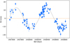 |
Fig. 5 Single-planet Keplerian fit to the RV data of TYC 2187-512-1 from CARMENES VIS. The orbital parameters are listed in the left column of Table 3. |
6.2.2 Gaussian process model
To obtain a consistent picture of the RV variations of TYC 2187-512-1, we used a model that describes the planet with a Keplerian, and the rotational modulation with a Gaussian process, as explained in Sect. 6.1. We performed an MCMC optimization of the Keplerian parameters and GP hyper-parameters with uninformative priors within bounds based on the single-planet fit, as tabulated in Appendix B. We employed 500 walkers and let them run for 700 steps each, discarding the first 200 samples as a burn-in phase. We checked that the process converged, and used a total of 81 354 accepted samples to compute distributions of the model parameters. The results are listed in the right column of Table 3; more detailed information about the underlying distributions of the MCMC samples is shown in Appendix C. A comparison of both columns in Table 3 shows that all planet parameters are fully consistent with those obtained from the single-planet model, but the GP model is favored strongly as indicated by the difference in the Bayesian information criterion (BIC) of −32. The RV curve of the combined model is shown in Fig. 6; both the planet and the stellar rotation are evidently reproduced well. This is further demonstrated in Figs. 7 and 8, which show the contributions of the GP and of the Keplerian to the observed RV separately. We note that the short-term variations represented by the GP maintain a zero mean on longer time scales as intended; thus, the GP does not add or subtract power from the planetary signal. We therefore adopt the best-fit parameters of the GP model listed in the right-hand column of Table 3 for the planet TYC 2187-512-1 b.
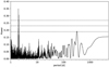
Figure 9 shows that no significant power remains at any frequency in the residuals of the GP model. The only peak with a false-alarm probability of only a few per cent is at 18.6 d, very close to the second harmonic of the rotation. We conclude that all our data on TYC 2187-512-1 are represented well by the “one planet plus rotational modulation” model.
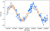 |
Fig. 6 Gaussian process model fit to the RV data of TYC 2187-512-1 from CARMENES VIS. The orbital parameters are listed in the right column of Table 3. Here and in the following figures the GP model and its 1er credibility range are shown in grey and brown, respectively. |
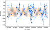 |
Fig. 7 Gaussian process model fit to the RV data of TYC 2187-512-1 from CARMENES VIS, as in Fig. 6, but with the planet orbit fit subtracted. This figure shows that the SHO model reproduces the ~40-day quasi-periodic variations very well, without introducing any power on longer time scales, which could affect the best-fit planet parameters. |
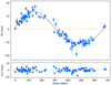 |
Fig. 8 Gaussian process model fit to the RV data of TYC 2187-512-1 from CARMENES VIS, as in Fig. 6, but with the Gaussian process model of the stellar variability subtracted and folded to the period of TYC 2187-512-1 b (691.90 d). |
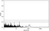 |
Fig. 9 GLS periodogram of the residuals of the GP model for TYC 2187-512-1. False-alarm probabilities of 0.1, 0.01, and 0.001 are shown as dashed horizontal lines. The scales of the axes are identical to Fig. 1 for better comparison. |
6.3 TZ Ari
6.3.1 Single-planet Keplerian fit
As for TYC 2187-512-1, we started by fitting a single-planet model to the RV data of TZ Ari. Here we used the combined data set from HIRES, HARPS, and CARMENES (see Sect. 4), and allowed for individual RV zero points and jitter terms for the three instruments. The best-fit parameters are listed in the left column of Table 4, and the data together with the best fit are shown in Fig. 10. A highly eccentric Keplerian with period ~770 d provides a reasonable fit to all data, albeit with a rather large seemingly white-noise scatter. As we will show in the next section, however, this scatter does bear the imprint of the 1.96-day rotation period, and can readily be modeled and explained by it. We thus ascribe the 770 d signal to a planet, TZ Arib.
6.3.2 Gaussian process model
Proceeding as with TYC 2187-512-1, we also modeled the RV data of TZ Ari with a GP, using the priors in Appendix B. Here we let 700 walkers run for 1000 steps each, discarded the first 500, and retained 118 702 samples for the computation of the model parameters and their confidence ranges. The results are shown in Figs. 11–14 and listed in the right column of Table 4, and more detailed information is again shown in Appendix C. Comparing the two columns in Table 4, there is good overall agreement between the two models, but with a ~10% lower value of K for the GP model. A closer inspection of the data reveals a correlation between K and the zero point of the HARPS RVs, which are clustered around the maximum of the RV curve (see Fig. 14, also noting the elongation of the distribution in the field “Kb, RV off3” in Fig. C.2). As the GP yields a fully consistent model (apparent in Fig. 14) and as this model is again strongly favored over the single-planet model (ΔBIC = −152), we adopted the corresponding parameters for TZ Arib as listed in the right-hand column of Table 4.
The residuals of the GP model for TZ Ari are shown in Fig. 15. The only peak exceeding the 10% false-alarm probability threshold, at 42.3 d, is probably an alias of the second harmonic of the rotation (1/42.3 + 1 ≈ 2/1.96). As in the previous case, we conclude that all available data on TZ Ari can be modeled with a single planet plus rotational modulation.
Single-planet Keplerian and Gaussian process model fit to the combined RV data of TZ Ari from HIRES, CARMENES VIS, and HARPS (labeled as 1, 2, and 3, respectively).
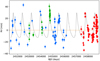 |
Fig. 10 Single-planet Keplerian fit to the RV data of TZ Ari from HIRES (blue), HARPS (green), and CARMENES VIS (red). The orbital parameters are listed in the left column of Table. |
6.3.3 Considering whether the 770-day signal could be due to activity cycles
While the modeling of the 770-day RV signal presented in the previous sections is fully compatible with a planetary origin, we also conducted additional checks to address the possibility that it could instead be caused by stellar activity cycles:
An RV signal induced by stellar activity would likely have a higher amplitude at shorter wavelengths, because it would be related to temperature variations. We therefore compared the amplitudes of the signal from the visible and infrared spectrographs of CARMENES with each other, but found agreement between the respective amplitudes (21.5 and 21.0 m s–1, respectively).
The combined RV data set (see Fig. 11) covers ten cycles without any noticeable change of either amplitude or phase. This is also apparent from the near-perfect folding of the RVs with phase (see Fig. 14). In contrast, activity cycles might vary in strength or duration, as observed in the Sun.
It might be expected that activity cycles would manifest themselves through, for example, the variability of the Hα line. However, the periodograms of CRX, dLW, and spectroscopic indicators described in Sect. 5 and shown in Appendix A do not show any significant power near 770 d.
The effect of activity cycles on the RVs would likely not only be a smooth periodic variation, but also a modulation of the short-term scatter with the phase of the cycle. We therefore subtracted the single-Keplerian fit of Fig. 10 – meant here to represent the smooth RV variations – from the data, and computed a GLS periodogram of the absolute values of the residuals. No excess power near 770 d was found, indicating that the RV scatter does not depend on the phase of the long-term variations.
No long-term photometric variations are observed in our SuperWASP photometry or in publicly available data from MEarth (Berta et al. 2012), with an upper limit of ~5 mmag on periods near 770 d. This is not a very constraining limit compared to photometric variations of the Sun, which are only on an order of 1 mmag, but achieving this precision with ground-based photometric monitoring would be very difficult.
Although none of these arguments by itself excludes activity cycles as a possible cause of the 770-day signal, the preponderance of the evidence strongly points to a planetary origin.
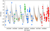 |
Fig. 11 Gaussian process model fit to the RV data of TZ Ari from HIRES (blue), HARPS (green), and CARMENES VIS (red). The orbital parameters are listed in the right column of Table 4. The rotational modulation of the RV is far too fast to be seen at any reasonable screen or print resolution; the full range of this variation is therefore seen as a grey band. We provide a zoom into a short section in Fig. 12. |
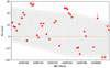 |
Fig. 12 Zoom onto the Gaussian process model fit to the RV data of TZ Ari shown in Fig. 11. The fast modulation with a period of 1.96 d is due to the stellar rotation. The long-term downward trend is part of the 770-day planetary orbit. |
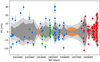 |
Fig. 13 Gaussian process model fit to the RV data of TZ Ari as in Fig. 11, but with the planet orbit fit subtracted. Together with Fig. 12, this figure shows that the SHO model reproduces the 1.96-day quasi-periodic variations very well, without introducing any power on longer time scales, which could affect the best-fit planet parameters. |
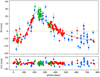 |
Fig. 14 Gaussian process model fit to the RV data of TZ Ari as in Fig. 11, but with the Gaussian process model of the stellar variability subtracted, and folded to the period of TZ Arib (771.36 d). |
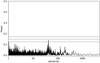 |
Fig. 15 GLS periodogram of the residuals of the GP model for TZ Ari. False-alarm probabilities of 0.1, 0.01, and 0.001 are shown as dashed horizontal lines. The scales of the axes are identical to Fig. 2 for better comparison. |
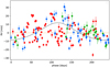 |
Fig. 16 Two-planet fit for TZ Ari from Feng et al. (2020). Their model of the 770 d-planet was subtracted, and the residuals phase-folded to the period of the putative second planet, 241.59 d. While the HIRES (blue) and HARPS (green) data weakly support this planet candidate, the CARMENES VIS (red) data rule out its existence. |
6.3.4 Considering a second planet in the system
The 770 d RV periodicity was already detected in the HIRES RV time series and was classified as a “signal requiring confirmation” by Butler et al. (2017). In the combined HIRES and HARPS data sets, Tuomi et al. (2019) identified three planet candidates with orbital periods of 773.4 d, 1.932 d, and 243.1 d; the first and third of these are also listed by Feng et al. (2020)4. The first of these candidates has now been established as a planet thanks to the larger, more precise, and better sampled CARMENES dataset, and to the arguments presented in Sect. 6.3.3. The second candidate is definitely spurious. It corresponds to the 1.96 d signal, which can firmly be attributed to rotational modulation because it is chromatic, involves variations in the line shape (dLW), and is accompanied by photometric variability, as well as periodic changes of the line indices (see Sect. 5.3).
To assess the reality of the 240 d planet candidate, we first note that the two-planet model of Feng et al. (2020) is incompatible with the CARMENES data (see Fig. 16). For a more thorough analysis, we extend the model of Sect. 6.3.2 by adding a second planet with a period constrained to P ∈ [240, 245] d, with all other parameters left free. The best-fit amplitude is found to be K = 0.95 + 1.05 m s–1, and thus compatible with zero. This demonstrates that there is no evidence for a planet in this period range in the combined data set.
We conclude that on the basis of the CARMENES data, we can firmly establish TZ Arib as a bona fide planet and we demonstrate that the previously suspected additional planet candidates are spurious.
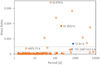 |
Fig. 17 Mass ratio-period relation for planets orbiting low-mass stars. The y-axis shows the mass ratio m/M* (for transiting planets) or m sin i/M* (for non-transiting planets). The dashed horizontal lines indicate the mass ratios of Saturn and Jupiter compared to the Sun. The open symbols designate planets orbiting hosts with 0.3 M⊙ < M* ≤ 0.55 M⊙, the filled symbols are for host masses M* ≤ 0.3 M⊙. Objects with small mass ratios, that is, terrestrial planets and super-Earths, are included for illustration, but not discussed further in the present paper. The data were compiled from the NASA Exoplanet Archive. |
7 Discussion
7.1 TYC 2187-512-1 b
The planet TYC 2187-512-1 b is about 10% more massive than Saturn; the eccentricity of its orbit is compatible with zero. With an insolation between that of Jupiter and Saturn (more precisely, about 2.5 times that of Saturn), TYC 2187-512-1 b could be physically quite similar to the gas giants in the Solar System. The system does in fact resemble a number of others with an early M host and a single Saturn-like planet in a long-period orbit (see Sect. 7.3 and Fig. 17).
7.2 TZ Arib
The companion of TZ Ari is much more uncommon: it is only the second known giant planet orbiting a host with M* ≤ 0.3 M⊙, along with GJ 3512 b (Morales et al. 2019) and not counting the candidate GJ 3512 c. The unusual nature of the GJ 3512 and TZ Ari systems is quite apparent in a diagram of planet mass, m, versus host mass, M*, where they are separated from other known systems by a gap of a factor of ~2 in M* or a factor of ~5 in m (see Fig. 1 in Quirrenbach et al. 2020, and Fig. 17). The orbits of TZ Arib and GJ3512b are rather similar: While the former has a longer period than the latter (771 d vs. 204 d), both have rather large and nearly identical eccentricity (0.46 and 0.44, respectively).
As noted in Sect. 2.2, the observational limit on v sin leads to Prot/ sin i* > 4.15 d. Combining this with the rotation period of 1.96 d, we conclude that the stellar rotation axis must be rather inclined, sin i* < 0.47. This means that TZ Ari b must have either a rather misaligned orbit or a mass of at least 0.45 MJup (if aligned), which is twice as great as the minimum mass, m sin i. This question will certainly be resolved once the full Gaia data, including astrometric orbit solutions, are published.
TZ Arib is also among the closest giant exoplanets to the Earth, which means that its angular orbital semi-major axis of 0.″27 is rather large. With a radius that should be about ten times larger than the Earth’s, the contrast between TZ Arib and its host is two orders of magnitudes more favorable than that of a terrestrial planet, which makes it a very suitable target for characterization by a future direct imaging mission. This will be particularly interesting because of the eccentric orbit, which gives rise to periodic variations of the insolation by a factor of more than seven.
The orbit-averaged insolation of TZ Arib is only about 30% that of Saturn. Its energy balance will therefore remain dominated by internal heat beyond an age of 10 Gyr (Linder et al. 2019). Consequently, the effective temperature of TZ Ari b will slowly approach its equilibrium value Teff ≈ 65 K, with a present value likely below 100 K. It is therefore no surprise that the planet was not discovered in the 8.7 µm survey of Gauza et al. (2021). Searches for reflected light will be more promising, with an expected contrast of order 3 × 10⁻⁸ between the planet and its host.
Giant planets (m sin i ≥ 0.5 MSat ≈ 0.15 MJup) in the CARMENES sample.
7.3 Giant planets in the CARMENES M-dwarf sample
The CARMENES survey was designed to provide statistical information on planetary systems of low-mass stars. In fact, it covers the mass range from the hydrogen burning limit at 0.07 M⊙ to the upper end of the M spectral class near 0.6 M⊙ rather uniformly (see Fig. 2 in Reiners et al. 2018). While a thorough statistical analysis has to await the completion of the survey, it is already possible to draw preliminary conclusions on the occurrence rate of giant planets in the sample. For the following discussion, we adopt a somewhat arbitrary definition of m sin i ≥ 0.5 MSat ≈ 0.15 MJup for this class. The twelve planets in the CARMENES sample of 387 M dwarfs (including those found independently) fulfilling this criterion are listed in Table 5. The entries in the table immediately provide a lower limit on the number of the giant planets in this sample. On the other hand, we can roughly estimate the completeness of this list as follows: So far, 160 stars have been observed at least 30 times during the survey, with RVs taken over a time span of more than 1 yr. A giant planet with m sin i ≥ 0.5MSat in a circular orbit with P ≤ 2 yr around a star with M* ≤ 0.5 M⊙ gives rise to a signal of K ≥ 5.4m s–1 and would thus have easily been found in any of these 160 RV curves, unless its presence is masked by strong stellar activity, which may be the case for up to ~25% of the stars (Tal-Or et al. 2018). We thus conclude that the completeness of Table 5 for periods up to two years is at least 0.75 · (160/387) ≈ 33%, and probably substantially higher because many additional stars have been observed already more than 20 times. The completeness drops towards longer periods because K ∝ P–1/3 and because many stars have now been monitored for two to three years.
From an inspection of Table 5 we can draw a few direct conclusions about the population of giant planets orbiting M dwarfs:
Giant planets exist around stars of all masses down to at least 0.12 M⊙, with orbital periods ranging from a few weeks to at least two decades.
While planets with m sin i ≥ 1 MJup appear to be rare (with GJ 876 b being the only one in the sample), “mass ratios” m sin i/M* larger than that of Jupiter and the Sun are actually quite common.
The observed orbital eccentricities range from values compatible with zero to e = 0.46.
At least three of the nine known systems in the CARMENES sample have multiple giant planets.
The inferred occurrence rate of M dwarfs hosting giant planets with periods up to 2 yr is 2–6%, with the limits representing the assumptions that the table is 100% or only 33% complete. This is somewhat lower than the corresponding number for FGK stars (roughly 10%, see e.g. Fernandes et al. 2019; Wittenmyer et al. 2020 and Table 1 in Winn & Fabrycky 2015), but the estimates come closer together if m sin i/M* is considered instead of m sin i.
As a cautionary remark, we note that the mass range below M* ~ 0.3 M⊙ remains poorly explored, with good RV coverage for only a few dozen stars resulting in two detections, namely GJ3512b and TZ Arib. Here, the completion of the CARMENES survey, and its extension that began in 2021, will provide statistical information on more than 350 nearby M stars. We are aiming at obtaining uniform detection limits, and we will perform detailed injection-retrieval experiments, extending the analysis of 71 CARMENES stars by Sabotta et al. (2021) to the whole sample.
7.4 Giant planets orbiting low-mass stars
To get a broader overview of the giant planet population orbiting low-mass stars, we compiled a list of these objects from the NASA Exoplanet Archive5. We note that objects with masses ranging from ~ 1 MJup to the low-mass stellar regime have nearly identical diameters, and therefore objects discovered by transit surveys without mass measurements are of little value for the following discussion. Starting from a database query for all planets with masses (or m sin i) known from radial velocities or transit timing variations, and with host mass M* ≤ 0.55 M⊙, we disregarded a few host stars with Teff > 4300 K (and thus obviously dubious mass estimates). We computed a “mass ratio” for each planet, which is either m/M* or m sin i/M*, depending on whether sin i is known or not. As the expectation value for a random orientation of the orbits  , which is rather close to one, we make no further attempt to place limits on sini for the non-transiting planets, and use m sin i and the mass ratio as defined here as good proxies for the underlying masses and “true” mass ratios.
Figure 17 shows the mass ratio for this sample of 112 planets, together with TYC 2187-512-1 b and TZ Arib, as a function of their orbital period. This figure makes it apparent that: (i) no “hot Jupiter” with a period of P ≤ 10 d and host mass of M* ≤ 0.55 M⊙ has been found thus far and that (ii) giant planets with longer periods of P ≥ 30 d and low-mass hosts are not uncommon. The two discoveries from the CARMENES Survey GJ3512b and TZ Arib demonstrate that this second statement remains true down to host masses of M* ≈ 0.15 M⊙, as mentioned in Sect. 7.3.
The period distribution of giant planets discovered in RV surveys of FGK stars shows a lack of objects in the range between 10 and 100 d, sometimes dubbed the “period valley” (Udry et al. 2003; Santerne et al. 2016), with higher occurences at shorter and at longer periods. No such valley is apparent in Fig. 17. The occurrence rate of hot Jupiters in samples of AFGK stars observed by Kepler and TESS is about 0.4%, with a slight, statistically insignificant tendency towards higher values at lower stellar masses (Zhou et al. 2019). This possible trend does not seem to continue into the M dwarf range, but the current absence of hot Jupiters from the M dwarf samples could also just be due to small number statistics. In Fig. 17, we also mark HATS-71 b, for which a mass of 0.37 ± 0.24 MJup and a radius of 1.024 ± 0.018 RJup have been measured (Bakos et al. 2020). These values are indicative of a hot and somewhat inflated Saturn, but also compatible with a hot Jupiter. More mass measurements of gas giants transiting hosts with masses M* ≤ 0.5 M⊙, together with RV surveys of larger M dwarf samples, are needed to ascertain whether the apparent differences between low-mass stars and FGK stars are genuine or due, rather, to the present small-number statistics.
7.5 Astrometric constraints
For stars with known parallax ϖ, the spectroscopic orbital parameters can directly be converted into a lower limit for the astrometric signature α, namely, the semi-major axis of the orbital ellipse projected onto the sky (Reffert & Quirrenbach 2011)6:
 (5)
(5)
For TYC 2187-512-1 b and TZ Ari b, we get αmin = 49.1 µas and αmin = 235 µas, respectively, well within the capabilities of the Gaia mission. It is indeed expected that Gaia will provide a rather complete census of giant planets orbiting dwarf stars in the Solar neighborhood with intermediate periods (Sozzetti et al. 2014; Reylé et al. 2021). This will likely include all planets in Table 5, except GJ 1148 b and GJ 15 Ac, which have a very small astrometric signature and a very long period, respectively. Since astrometric orbit solutions include the inclination, the dynamical masses of these planets will be known as soon as the Gaia orbits are published.
Even astrometric non-detections can provide useful constraints on spectroscopic orbits, as it is always possible to infer a lower limit to sin i from them. This requires access to the individual astrometric measurements, which are not yet available for Gaia. However, the published data releases contain information on the astrometric orbit in the form of the parameter ϵi, the “excess source noise” quantifying the residuals from the standard five-parameter astrometric fit (Lindegren et al. 2012, 2016). While caution has to be exercised in interpreting ϵi for individual stars, the presence of a companion with a significant signature will usually lead to a correspondingly high value of ϵi. An inspection of ϵi in Gaia EDR3 for the stars in Table 5 reveals that they are all significantly different from zero, but never larger than 1 mas. This means that it is highly unlikely that any face-on stellar binaries have crept into this list. In addition, even inclinations making the companions brown dwarfs are highly unlikely (sin i < 0.07, corresponding to p < 0.25% in all but one cases), so that the tabulated objects can safely be considered gas giant planets.
7.6 Planet formation scenarios
The formation of rocky planets orbiting very low-mass stars such as TRAPPIST-1 (Gillon et al. 2017) and Teegarden’s Star (Zechmeister et al. 2019) can be explained with models based on the planetesimal accretion (Miguel et al. 2020) or pebble accretion (Schoonenberg et al. 2019) paradigms. It is very difficult, however, to incorporate the formation of gas giants in these scenarios (Morales et al. 2019), because a high migration rate is expected for rocky cores forming in the disks of late M dwarfs. Artificially reducing the speed of type I migration may point towards a solution of this conundrum (Burn et al. 2021), but it is also plausible that the dominant formation channel of these planets is through gravitational instabilities in their natal disk (Kratter & Lodato 2016). This possibility was explored by Mercer & Stamatellos (2020), who found that disk fragmentation is a viable pathway provided that the initial disk is sufficiently large, namely, about 30% of the stellar mass. In this context, it is worth noting that the “mass ratio”, m sin i/M*, of objects such as GJ3512b and TZ Arib is comparable to that of a low-mass brown dwarf around a Sun-like star, or to the pair of brown dwarfs orbiting the K giant v Oph (Quirrenbach et al. 2019), which may also have formed via disk instabilities. Around solartype stars, there are indeed indications for two separate giant planet populations whose occurrence rates have different dependencies on stellar metallicity: planets below ~4 MJup follow a positive metallicity-occurrence relation, whereas planets above this mass are found around host stars with a wide range of metallicities (Santos et al. 2017; Schlaufman 2018). The former trend is expected from a core accretion scenario, whereas the latter is consistent with disk fragmentation. More extensive surveys providing better statistics of the giant planet population over a large range of host star masses would help clarify this issue. Trends of planet occurrence rate with host star metallicity could also help to distinguish between different formation pathways. This possibility lends added urgency to a resolution of the remaining uncertainties in the determination of [Fe/H] in M dwarfs (see the discussions in Passegger et al. 2022 and Marfil et al. 2021). An alternative route would be the exploitation of Vanadium as a proxy of M dwarf metallicities (Shan et al. 2021).
The high eccentricity of the orbits of GJ 3512 b and TZ Ari b could be a result of past planet-planet interaction in a multiple system (Ida et al. 2013; Carrera et al. 2019). The RV data of GJ 3512 do indeed show a long-term modulation indicative of a second outer planet candidate with a period of at least four years (Morales et al. 2019). In contrast, there is no indication of any long-period trend in the RVs of TZ Ari (see Figs. 11 and 13). The time series covers 20 years, but the intrinsic RV variability of the star limits the ability to detect long-period planets. Because of the proximity of the star, a search for an acceleration in the Gaia astrometric data set will be the most sensitive test for the presence of a third body in the system.
8 Conclusions
We present two Saturn-mass planets in wide orbits around M dwarfs, TYC2187-512-1 b and TZ Arib, whose parameters can be established from RV measurements even in the presence of a rather strong signature of stellar rotation in these data. While TYC 2187-512-1 b, which orbits an early M star, is not unusual as a number of other planets with similar properties are known, TZ Arib is only the second confirmed giant planet orbiting a star with mass M* ≤ 0.3 M⊙. In fact, the mass of TZ Ari is only 0.15 M⊙, similar to that of GJ3512, the other low-mass host of a gas giant planet. These two systems occupy an extreme region of the planet mass / host mass parameter space, where disk fragmentation appears to be a more likely formation mechanism than build-up of a core through planetesimal or pebble accretion.
The orbits of both GJ 3512 b and TZ Ari b are rather eccentric (e = 0.44 and e = 0.46, respectively), which could be explained if the planets reside in multiple systems. Whereas a candidate outer planet, GJ 3512 c, has been identified in the first case, there is no indication for an additional companion of TZ Ari in the available data.
We infer an occurrence rate of giant planets orbiting M dwarfs with periods up to two years in the range between 2 to 6%. The completion of the CARMENES survey, together with the release of astrometric orbit fits from Gaia, will place tighter bounds on this number. The combination of information from RV surveys and Gaia will further improve our understanding of the architectures of M star systems, as the former are more sensitive to close-in planets and the latter to outer companions.
Acknowledgements
CARMENES is an instrument for the Centro Astronómico Hispano-Alemán (CAHA) at Calar Alto (Almería, Spain), operated jointly by the Junta de Andalucía and the Instituto de Astrofísica de Andalucía (CSIC). CARMENES was funded by the Max-Planck-Gesellschaft (MPG), the Consejo Superior de Investigaciones Científicas (CSIC), the Ministerio de Economía y Competitividad (MINECO) and the European Regional Development Fund (ERDF) through projects FICTS-2011-02, ICTS-2017-07-CAHA-4, and CAHA16-CE-3978, and the members of the CARMENES Consortium (Max-Planck-Institut für Astronomie, Instituto de Astrofísica de Andalucía, Landessternwarte Königstuhl, Institut de Ciències de l’Espai, Institut für Astrophysik Göttingen, Universidad Complutense de Madrid, Thüringer Landessternwarte Tautenburg, Instituto de Astrofísica de Canarias, Hamburger Sternwarte, Centro de Astrobiología and Centro Astronómico Hispano-Alemán), with additional contributions by the MINECO, the Deutsche Forschungsgemeinschaft through the Major Research Instrumentation Program and Research Unit FOR2544 “Blue Planets around Red Stars”, the Klaus Tschira Stiftung, the states of Baden-Württemberg and Niedersachsen, and by the Junta de Andalucia. We acknowledge financial support from NASA through grant NNX17AG24G. We acknowledge financial support from the Agencia Estatal de Investigación of the Ministerio de Ciencia, Innovación y Universidades through projects PID2019-110689RB-100, PID2019-109522GB-C5[1:4], PID2019-107061GB-C64 and the Centre of Excellence “Severo Ochoa”, Instituto de Astrofisica de Andalucia (SEV-2017-0709). We further acknowledge support by the BNSF program “VIHREN-2021” project No. KIJ-06-DB/5. Based on data from the CARMENES data archive at CAB (CSIC-INTA). Data were partly collected with the 150 and 90 cm telescopes at the Observatorio de Sierra Nevada (OSN) operated by the Instituto de Astrofísica de Andalucía (IAA-CSIC). This work makes use of observations from the Las Cumbres Observatory global telescope network. This research has made use of the NASA Exoplanet Archive, which is operated by the California Institute of Technology, under contract with the National Aeronautics and Space Administration under the Exoplanet Exploration Program. We thank the referee, Alexis Heitzmann, for his careful reading of the manuscript and his helpful comments.
Appendix A Periodograms of spectroscopic indicators
 |
A.1 GLS periodogram of the dLW time series of TYC 2187-512-1 from CARMENES. The prominent peak at 39.1 d indicates the rotation period. False-alarm probabilities of 0.1, 0.01, and 0.001 are shown as dashed horizontal lines. |
 |
A.2 GLS periodogram of the Hα line index time series of TYC 2187-512-1 from CARMENES. The prominent peak at 39.9 d indicates the rotation period. False-alarm probabilities of 0.1, 0.01, and 0.001 are shown as dashed horizontal lines. |
 |
A.3 GLS periodogram of the CRX time series of TZ Ari from CARMENES. The prominent peak at 1.96 d indicates the rotation period. False-alarm probabilities of 0.1, 0.01, and 0.001 are shown as dashed horizontal lines. |
 |
A.4 GLS periodogram of the Ha line index time series of TZ Ari from CARMENES. The strongest peak at 1.94 d is not significant, but it corresponds to the rotation period inferred from the other diagnostics. False-alarm probabilities of 0.1, 0.01, and 0.001 are shown as dashed horizontal lines. |
 |
A.5 GLS periodogram of an average of the three Ca II IRT line index time series of TZAri from CARMENES. The strongest peak at 1.95 d is not significant, but it corresponds to the rotation period inferred from the other diagnostics. False-alarm probabilities of 0.1, 0.01, and 0.001 are shown as dashed horizontal lines. |
Appendix B Gaussian process priors
Appendix C Corner plots
 |
C.1 Corner plot for the Gaussian process model fit to the RV data of TYC 2187-512-1 from CARMENES VIS shown in Fig. 6 and in the right column of Table 3 |
 |
C.2 Corner plot for the Gaussian process model fit to the RV data of TZ Ari from HIRES, CARMENES VIS, and HARPS shown in Fig. 11 and in the right column of Table 4. |
References
- Alonso-Floriano, F.J., Morales, J.C., Caballero, J.A., et al. 2015, A&A, 577, A128 [NASA ADS] [CrossRef] [EDP Sciences] [Google Scholar]
- Astudillo-Defru, N., Delfosse, X., Bonfils, X., et al. 2017, A&A, 600, A13 [NASA ADS] [CrossRef] [EDP Sciences] [Google Scholar]
- Bakos, G.Ä., Bayliss, D., Bento, J., et al. 2020, AJ, 159, 267 [NASA ADS] [CrossRef] [Google Scholar]
- Berta, Z.K., Irwin, J., Charbonneau, D., Burke, C.J., & Falco, E.E. 2012, AJ, 144, 145 [NASA ADS] [CrossRef] [Google Scholar]
- Bonfils, X., Delfosse, X., Udry, S., et al. 2013, A&A, 549, A109 [NASA ADS] [CrossRef] [EDP Sciences] [Google Scholar]
- Boro Saikia, S., Marvin, C.J., Jeffers, S.V., et al. 2018, A&A, 616, A108 [NASA ADS] [CrossRef] [EDP Sciences] [Google Scholar]
- Brown, T.M., Baliber, N., Bianco, F.B., et al. 2013, PASP, 125, 1031 [NASA ADS] [CrossRef] [Google Scholar]
- Burn, R., Schlecker, M., Mordasini, C., et al. 2021, A&A, 656, A72 [NASA ADS] [CrossRef] [EDP Sciences] [Google Scholar]
- Butler, R.P., Vogt, S.S., Laughlin, G., et al. 2017, AJ, 153, 208 [NASA ADS] [CrossRef] [Google Scholar]
- Caballero, J.A., Cortés-Contreras, M., Alonso-Floriano, F.J., et al. 2016a, in 19th Cambridge Workshop on Cool Stars, Stellar Systems, and the Sun (CS19), 148 [Google Scholar]
- Caballero, J.A., Guàrdia, J., Lopez del Fresno, M., et al. 2016b, SPIE Conf. Ser., 9910, 99100E [Google Scholar]
- Caffau, E., Ludwig, H.-G., Steffen, M., Freytag, B., & Bonifacio, P. 2011, Sol. Phys., 268, 255 [Google Scholar]
- Carrera, D., Raymond, S.N., & Davies, M.B. 2019, A&A, 629, L7 [NASA ADS] [CrossRef] [EDP Sciences] [Google Scholar]
- Cifuentes, C., Caballero, J.A., Cortés-Contreras, M., et al. 2020, A&A, 642, A115 [NASA ADS] [CrossRef] [EDP Sciences] [Google Scholar]
- Collins, K.A., Kielkopf, J.F., Stassun, K.G., & Hessman, F.V. 2017, AJ, 153, 77 [NASA ADS] [CrossRef] [Google Scholar]
- Colome, J., & Ribas, I. 2006, IAU Special Session, 6, 11 [Google Scholar]
- Cortés-Contreras, M., Dominguez-Fernândez, A.J., Caballero, J.A., et al. 2020, in XIV.0 Scientific Meeting (virtual) of the Spanish Astronomical Society, 131 [Google Scholar]
- Delfosse, X., Forveille, T., Mayor, M., et al. 1998, A&A, 338, L67 [Google Scholar]
- Diez Alonso, E., Caballero, J.A., Montes, D., et al. 2019, A&A, 621, A126 [NASA ADS] [CrossRef] [EDP Sciences] [Google Scholar]
- Dressing, C.D., & Charbonneau, D. 2013, ApJ, 767, 95 [NASA ADS] [CrossRef] [Google Scholar]
- Dumusque, X., Boisse, I., & Santos, N.C. 2014, ApJ, 796, 132 [NASA ADS] [CrossRef] [Google Scholar]
- Feng, Y.K., Wright, J.T., Nelson, B., et al. 2015, ApJ, 800, 22 [NASA ADS] [CrossRef] [Google Scholar]
- Feng, F., Shectman, S.A., Clement, M.S., et al. 2020, ApJS, 250, 29 [NASA ADS] [CrossRef] [Google Scholar]
- Fernandes, R.B., Mulders, G.D., Pascucci, I., Mordasini, C., & Emsenhuber, A. 2019, ApJ, 874, 81 [NASA ADS] [CrossRef] [Google Scholar]
- Foreman-Mackey, D., Agol, E., Ambikasaran, S., & Angus, R. 2017, AJ, 154, 220 [Google Scholar]
- Fuhrmeister, B., Czesla, S., Schmitt, J.H.M.M., et al. 2019, A&A, 623, A24 [NASA ADS] [CrossRef] [EDP Sciences] [Google Scholar]
- Gaia Collaboration (Brown, A.G.A., et al.) 2021, A&A, 649, A1 [NASA ADS] [CrossRef] [EDP Sciences] [Google Scholar]
- Gaidos, E., Mann, A.W., Lépine, S., et al. 2014, MNRAS, 443, 2561 [NASA ADS] [CrossRef] [Google Scholar]
- Gauza, B., Béjar, V.J.S., Rebolo, R., et al. 2021, ApJ, 923, 119 [NASA ADS] [CrossRef] [Google Scholar]
- Gillon, M., Triaud, A.H.M.J., Demory, B.-O., et al. 2017, Nature, 542, 456 [NASA ADS] [CrossRef] [Google Scholar]
- Gliese, W. 1969, Veroeffentlichungen des Astronomischen Rechen-Instituts Heidelberg, 22, 1 [NASA ADS] [Google Scholar]
- Haywood, R.D., Collier Cameron, A., Queloz, D., et al. 2014, MNRAS, 443, 2517 [NASA ADS] [CrossRef] [Google Scholar]
- Houdebine, É.R., Mullan, D.J., Doyle, J.G., et al. 2019, AJ, 158, 56 [NASA ADS] [CrossRef] [Google Scholar]
- Howard, A.W., Johnson, J.A., Marcy, G.W., et al. 2010, ApJ, 721, 1467 [NASA ADS] [CrossRef] [Google Scholar]
- Ida, S., Lin, D.N.C., & Nagasawa, M. 2013, ApJ, 775, 42 [NASA ADS] [CrossRef] [Google Scholar]
- Jeffers, S.V., Schöfer, P., Lamert, A., et al. 2018, A&A, 614, A76 [NASA ADS] [CrossRef] [EDP Sciences] [Google Scholar]
- Johnson, J.A., Aller, K.M., Howard, A.W., & Crepp, J.R. 2010a, PASP, 122, 905 [NASA ADS] [CrossRef] [Google Scholar]
- Johnson, J.A., Howard, A.W., Marcy, G.W., et al. 2010b, PASP, 122, 149 [NASA ADS] [Google Scholar]
- Kratter, K., & Lodato, G. 2016, ARA&A, 54, 271 [NASA ADS] [CrossRef] [Google Scholar]
- Kunkel, W.E. 1968, Information Bull. Variab. Stars, 294, 1 [Google Scholar]
- Lafarga, M., Ribas, I., Lovis, C., et al. 2020, A&A, 636, A36 [NASA ADS] [CrossRef] [EDP Sciences] [Google Scholar]
- Lafarga, M., Ribas, I., Reiners, A., et al. 2021, A&A, 652, A28 [NASA ADS] [CrossRef] [EDP Sciences] [Google Scholar]
- Lehtinen, J., Jetsu, L., Hackman, T., Kajatkari, P., & Henry, G.W. 2012, A&A, 542, A38 [NASA ADS] [CrossRef] [EDP Sciences] [Google Scholar]
- Lépine, S., Hilton, E.J., Mann, A.W., et al. 2013, AJ, 145, 102 [CrossRef] [Google Scholar]
- Lindegren, L., Lammers, U., Hobbs, D., et al. 2012, A&A, 538, A78 [NASA ADS] [CrossRef] [EDP Sciences] [Google Scholar]
- Lindegren, L., Lammers, U., Bastian, U., et al. 2016, A&A, 595, A4 [NASA ADS] [CrossRef] [EDP Sciences] [Google Scholar]
- Linder, E.F., Mordasini, C., Mollière, P., et al. 2019, A&A, 623, A85 [NASA ADS] [CrossRef] [EDP Sciences] [Google Scholar]
- Manara, C.F., Morbidelli, A., & Guillot, T. 2018, A&A, 618, L3 [NASA ADS] [CrossRef] [EDP Sciences] [Google Scholar]
- Marcy, G.W., Butler, R.P., Vogt, S.S., Fischer, D., & Lissauer, J.J. 1998, ApJ, 505, L147 [NASA ADS] [CrossRef] [Google Scholar]
- Marfil, E., Tabernero, H.M., Montes, D., et al. 2021, A&A, 656, A162 [NASA ADS] [CrossRef] [EDP Sciences] [Google Scholar]
- Mayor, M., Pepe, F., Queloz, D., et al. 2003, The Messenger, 114, 20 [NASA ADS] [Google Scholar]
- McCully, C., Volgenau, N.H., Harbeck, D.-R., et al. 2018, SPIE. Conf. Ser., 10707, 107070K [NASA ADS] [Google Scholar]
- Mercer, A., & Stamatellos, D. 2020, A&A, 633, A116 [NASA ADS] [CrossRef] [EDP Sciences] [Google Scholar]
- Meyer, M. 2017, PhD thesis, Universität Hamburg, Germany [Google Scholar]
- Miguel, Y., Cridland, A., Ormel, C.W., Fortney, J.J., & Ida, S. 2020, MNRAS, 491, 1998 [NASA ADS] [Google Scholar]
- Morales, J.C., Mustill, A.J., Ribas, I., et al. 2019, Science, 365, 1441 [NASA ADS] [CrossRef] [Google Scholar]
- Newton, E.R., Irwin, J., Charbonneau, D., et al. 2017, ApJ, 834, 85 [NASA ADS] [CrossRef] [Google Scholar]
- Passegger, V.M., Schweitzer, A., Shulyak, D., et al. 2019, A&A, 627, A161 [NASA ADS] [CrossRef] [EDP Sciences] [Google Scholar]
- Passegger, V.M., Bello-Garcia, A., Ordieres-Meré, J., et al. 2022, A&A, 658, A194 [NASA ADS] [CrossRef] [EDP Sciences] [Google Scholar]
- Perdelwitz, V., Mittag, M., Tal-Or, L., et al. 2021, A&A, 652, A116 [NASA ADS] [CrossRef] [EDP Sciences] [Google Scholar]
- Pollacco, D.L., Skillen, I., Collier Cameron, A., et al. 2006, PASP, 118, 1407 [NASA ADS] [CrossRef] [Google Scholar]
- Popinchalk, M., Faherty, J.K., Kiman, R., et al. 2021, ApJ, 916, 77 [NASA ADS] [CrossRef] [Google Scholar]
- Quirrenbach, A., Amado, P.J., Caballero, J.A., et al. 2014, Proc. SPIE Conf. Ser., 9147, 91471F [NASA ADS] [CrossRef] [Google Scholar]
- Quirrenbach, A., Amado, P.J., Caballero, J.A., et al. 2016, SPIE Conf. Seri., 9908, 990812 [NASA ADS] [Google Scholar]
- Quirrenbach, A., Amado, P.J., Ribas, I., et al. 2018, Proc. SPIE Conf. Ser., 10702, 107020W [NASA ADS] [Google Scholar]
- Quirrenbach, A., Trifonov, T., Lee, M.H., & Reffert, S. 2019, A&A, 624, A18 [NASA ADS] [CrossRef] [EDP Sciences] [Google Scholar]
- Quirrenbach, A., CARMENES Consortium, Amado, P.J., et al. 2020, SPIE Conf. Ser., 11447, 114473C [NASA ADS] [Google Scholar]
- Rajpaul, V., Aigrain, S., Osborne, M.A., Reece, S., & Roberts, S. 2015, MNRAS, 452, 2269 [NASA ADS] [CrossRef] [Google Scholar]
- Reffert, S., & Quirrenbach, A. 2011, A&A, 527, A140 [NASA ADS] [CrossRef] [EDP Sciences] [Google Scholar]
- Reffert, S., Bergmann, C., Quirrenbach, A., Trifonov, T., & Künstler, A. 2015, A&A, 574, A116 [NASA ADS] [CrossRef] [EDP Sciences] [Google Scholar]
- Reiners, A., Zechmeister, M., Caballero, J.A., et al. 2018, A&A, 612, A49 [NASA ADS] [CrossRef] [EDP Sciences] [Google Scholar]
- Reylé, C., Jardine, K., Fouqué, P., et al. 2021, A&A, 650, A201 [Google Scholar]
- Ribas, I., Tuomi, M., Reiners, A., et al. 2018, Nature, 563, 365 [Google Scholar]
- Rodriguez, E., Garcia, J.M., Costa, V., et al. 2010, MNRAS, 408, 2149 [NASA ADS] [CrossRef] [Google Scholar]
- Rodriguez Martinez, R., Lopez, L.A., Shappee, B.J., et al. 2020, ApJ, 892, 144 [NASA ADS] [CrossRef] [Google Scholar]
- Sabotta, S., Schlecker, M., Chaturvedi, P., et al. 2021, A&A, 653, A114 [NASA ADS] [CrossRef] [EDP Sciences] [Google Scholar]
- Santerne, A., Moutou, C., Tsantaki, M., et al. 2016, A&A, 587, A64 [NASA ADS] [CrossRef] [EDP Sciences] [Google Scholar]
- Santos, N.C., Adibekyan, V., Figueira, P., et al. 2017, A&A, 603, A30 [NASA ADS] [CrossRef] [EDP Sciences] [Google Scholar]
- Schlaufman, K.C. 2018, ApJ, 853, 37 [NASA ADS] [CrossRef] [Google Scholar]
- Schöfer, P., Jeffers, S.V., Reiners, A., et al. 2019, A&A, 623, A44 [NASA ADS] [CrossRef] [EDP Sciences] [Google Scholar]
- Schoonenberg, D., Liu, B., Ormel, C.W., & Dorn, C. 2019, A&A, 627, A149 [NASA ADS] [CrossRef] [EDP Sciences] [Google Scholar]
- Schweitzer, A., Passegger, V.M., Cifuentes, C., et al. 2019, A&A, 625, A68 [NASA ADS] [CrossRef] [EDP Sciences] [Google Scholar]
- Shan, Y., Reiners, A., Fabbian, D., et al. 2021, A&A, 654, A118 [NASA ADS] [CrossRef] [EDP Sciences] [Google Scholar]
- Skrutskie, M.F., Cutri, R.M., Stiening, R., et al. 2006, AJ, 131, 1163 [NASA ADS] [CrossRef] [Google Scholar]
- Sozzetti, A., Giacobbe, P., Lattanzi, M.G., et al. 2014, MNRAS, 437, 497 [NASA ADS] [CrossRef] [Google Scholar]
- Suârez Mascareno, A., Rebolo, R., & Gonzalez Hernandez, J.I. 2016, A&A, 595, A12 [NASA ADS] [CrossRef] [EDP Sciences] [Google Scholar]
- Tabernero, H.M., Marfil, E., Montes, D., & Gonzalez Hernandez, J.I. 2022, A&A, 657, A66 [NASA ADS] [CrossRef] [EDP Sciences] [Google Scholar]
- Tal-Or, L., Zechmeister, M., Reiners, A., et al. 2018, A&A, 614, A122 [NASA ADS] [CrossRef] [EDP Sciences] [Google Scholar]
- Tal-Or, L., Trifonov, T., Zucker, S., Mazeh, T., & Zechmeister, M. 2019, MNRAS, 484, L8 [Google Scholar]
- Tamuz, O., Mazeh, T., & Zucker, S. 2005, MNRAS, 356, 1466 [Google Scholar]
- Trifonov, T. 2019, Astrophysics Source Code Library [record ascl:1986.884] [Google Scholar]
- Trifonov, T., Kürster, M., Zechmeister, M., et al. 2018, A&A, 609, A117 [NASA ADS] [CrossRef] [EDP Sciences] [Google Scholar]
- Trifonov, T., Lee, M.H., Kürster, M., et al. 2020a, A&A, 638, A16 [NASA ADS] [CrossRef] [EDP Sciences] [Google Scholar]
- Trifonov, T., Tal-Or, L., Zechmeister, M., et al. 2020b, A&A, 636, A74 [NASA ADS] [CrossRef] [EDP Sciences] [Google Scholar]
- Tuomi, M., Jones, H.R.A., Butler, R.P., et al. 2019, AAS Journals, submitted [Google Scholar]
- Udry, S., Mayor, M., & Santos, N.C. 2003, A&A, 407, 369 [NASA ADS] [CrossRef] [EDP Sciences] [Google Scholar]
- Vida, K., Kriskovics, L., Olâh, K., et al. 2016, A&A, 590, A11 [NASA ADS] [CrossRef] [EDP Sciences] [Google Scholar]
- Vogt, S.S., Allen, S.L., Bigelow, B.C., et al. 1994, SPIE Conf. Ser., 2198, 362 [NASA ADS] [Google Scholar]
- Winn, J.N., & Fabrycky, D.C. 2015, ARA&A, 53, 409 [NASA ADS] [CrossRef] [Google Scholar]
- Wittenmyer, R.A., Wang, S., Horner, J., et al. 2020, MNRAS, 492, 377 [NASA ADS] [CrossRef] [Google Scholar]
- Zechmeister, M., & Kürster, M. 2009, A&A, 496, 577 [CrossRef] [EDP Sciences] [Google Scholar]
- Zechmeister, M., Reiners, A., Amado, P.J., et al. 2018, A&A, 609, A12 [NASA ADS] [CrossRef] [EDP Sciences] [Google Scholar]
- Zechmeister, M., Dreizler, S., Ribas, I., et al. 2019, A&A, 627, A49 [NASA ADS] [EDP Sciences] [Google Scholar]
- Zhou, G., Huang, C.X., Bakos, G.Ä., et al. 2019, AJ, 158, 141 [NASA ADS] [CrossRef] [Google Scholar]
CARMENES identifier from the Carmencita database, see Caballero et al. (2016a).
Note that there is a sign error in the equivalent widths given by Gaidos et al. (2014) and in the associated electronic tables.
A line index l can be converted into a pseudo-equivalent width of the line with the relation pEW = (1 - l)Δλ.
Note that these authors use a nomenclature for the periodic signals that deviates from the original one.
Note that these authors use a nomenclature for the periodic signals that deviates from the original one.
All Tables
Single-planet Keplerian and Gaussian process model fit to the RV data of TYC 2187-512-1 from CARMENES VIS.
Single-planet Keplerian and Gaussian process model fit to the combined RV data of TZ Ari from HIRES, CARMENES VIS, and HARPS (labeled as 1, 2, and 3, respectively).
All Figures
|
Fig. 1 GLS periodogram of the RV time series of TYC 2187-512-1 from CARMENES. The prominent peak at 696 d can be attributed to a planet. The marginally significant peak at 7.15 d and its alias at 1.15 d are due to the window function of the sampling. The insignificant but noticeable power near 40 d corresponds to the rotation period of the star. False-alarm probabilities of 0.1, 0.01, and 0.001 are shown as dashed horizontal lines. |
| In the text | |
|
Fig. 2 GLS periodogram of the combined RV time series of TZ Ari from CARMENES, HIRES, and HARPS. The prominent peaks at 781 d and 1.96 d correspond to a planet and to the stellar rotation period, respectively. False-alarm probabilities of 0.1, 0.01, and 0.001 are shown as dashed horizontal lines. |
| In the text | |
|
Fig. 3 Differential photometry of TYC 2187-512-1, phase-folded to P = 40.0203 d. Each data point represents measurements averaged over one night. SuperWASP data are shown as blue circles, and OSN R-band data are represented by green triangles. Within each of the two time series, the symbols change from light to dark with progressing time. See the text for more details. |
| In the text | |
|
Fig. 4 Photometry and Hα index of TYC 2187-512-1, phase-folded to P = 40.0203 d and averaged into 20 equally spaced phase bins. The photometric data from SuperWASP and OSN (R-band) are shown in blue, and the Hα line index from CARMENES is shown in orange. |
| In the text | |
|
Fig. 5 Single-planet Keplerian fit to the RV data of TYC 2187-512-1 from CARMENES VIS. The orbital parameters are listed in the left column of Table 3. |
| In the text | |
|
Fig. 6 Gaussian process model fit to the RV data of TYC 2187-512-1 from CARMENES VIS. The orbital parameters are listed in the right column of Table 3. Here and in the following figures the GP model and its 1er credibility range are shown in grey and brown, respectively. |
| In the text | |
|
Fig. 7 Gaussian process model fit to the RV data of TYC 2187-512-1 from CARMENES VIS, as in Fig. 6, but with the planet orbit fit subtracted. This figure shows that the SHO model reproduces the ~40-day quasi-periodic variations very well, without introducing any power on longer time scales, which could affect the best-fit planet parameters. |
| In the text | |
|
Fig. 8 Gaussian process model fit to the RV data of TYC 2187-512-1 from CARMENES VIS, as in Fig. 6, but with the Gaussian process model of the stellar variability subtracted and folded to the period of TYC 2187-512-1 b (691.90 d). |
| In the text | |
|
Fig. 9 GLS periodogram of the residuals of the GP model for TYC 2187-512-1. False-alarm probabilities of 0.1, 0.01, and 0.001 are shown as dashed horizontal lines. The scales of the axes are identical to Fig. 1 for better comparison. |
| In the text | |
|
Fig. 10 Single-planet Keplerian fit to the RV data of TZ Ari from HIRES (blue), HARPS (green), and CARMENES VIS (red). The orbital parameters are listed in the left column of Table. |
| In the text | |
|
Fig. 11 Gaussian process model fit to the RV data of TZ Ari from HIRES (blue), HARPS (green), and CARMENES VIS (red). The orbital parameters are listed in the right column of Table 4. The rotational modulation of the RV is far too fast to be seen at any reasonable screen or print resolution; the full range of this variation is therefore seen as a grey band. We provide a zoom into a short section in Fig. 12. |
| In the text | |
|
Fig. 12 Zoom onto the Gaussian process model fit to the RV data of TZ Ari shown in Fig. 11. The fast modulation with a period of 1.96 d is due to the stellar rotation. The long-term downward trend is part of the 770-day planetary orbit. |
| In the text | |
|
Fig. 13 Gaussian process model fit to the RV data of TZ Ari as in Fig. 11, but with the planet orbit fit subtracted. Together with Fig. 12, this figure shows that the SHO model reproduces the 1.96-day quasi-periodic variations very well, without introducing any power on longer time scales, which could affect the best-fit planet parameters. |
| In the text | |
|
Fig. 14 Gaussian process model fit to the RV data of TZ Ari as in Fig. 11, but with the Gaussian process model of the stellar variability subtracted, and folded to the period of TZ Arib (771.36 d). |
| In the text | |
|
Fig. 15 GLS periodogram of the residuals of the GP model for TZ Ari. False-alarm probabilities of 0.1, 0.01, and 0.001 are shown as dashed horizontal lines. The scales of the axes are identical to Fig. 2 for better comparison. |
| In the text | |
|
Fig. 16 Two-planet fit for TZ Ari from Feng et al. (2020). Their model of the 770 d-planet was subtracted, and the residuals phase-folded to the period of the putative second planet, 241.59 d. While the HIRES (blue) and HARPS (green) data weakly support this planet candidate, the CARMENES VIS (red) data rule out its existence. |
| In the text | |
|
Fig. 17 Mass ratio-period relation for planets orbiting low-mass stars. The y-axis shows the mass ratio m/M* (for transiting planets) or m sin i/M* (for non-transiting planets). The dashed horizontal lines indicate the mass ratios of Saturn and Jupiter compared to the Sun. The open symbols designate planets orbiting hosts with 0.3 M⊙ < M* ≤ 0.55 M⊙, the filled symbols are for host masses M* ≤ 0.3 M⊙. Objects with small mass ratios, that is, terrestrial planets and super-Earths, are included for illustration, but not discussed further in the present paper. The data were compiled from the NASA Exoplanet Archive. |
| In the text | |
|
A.1 GLS periodogram of the dLW time series of TYC 2187-512-1 from CARMENES. The prominent peak at 39.1 d indicates the rotation period. False-alarm probabilities of 0.1, 0.01, and 0.001 are shown as dashed horizontal lines. |
| In the text | |
|
A.2 GLS periodogram of the Hα line index time series of TYC 2187-512-1 from CARMENES. The prominent peak at 39.9 d indicates the rotation period. False-alarm probabilities of 0.1, 0.01, and 0.001 are shown as dashed horizontal lines. |
| In the text | |
|
A.3 GLS periodogram of the CRX time series of TZ Ari from CARMENES. The prominent peak at 1.96 d indicates the rotation period. False-alarm probabilities of 0.1, 0.01, and 0.001 are shown as dashed horizontal lines. |
| In the text | |
|
A.4 GLS periodogram of the Ha line index time series of TZ Ari from CARMENES. The strongest peak at 1.94 d is not significant, but it corresponds to the rotation period inferred from the other diagnostics. False-alarm probabilities of 0.1, 0.01, and 0.001 are shown as dashed horizontal lines. |
| In the text | |
|
A.5 GLS periodogram of an average of the three Ca II IRT line index time series of TZAri from CARMENES. The strongest peak at 1.95 d is not significant, but it corresponds to the rotation period inferred from the other diagnostics. False-alarm probabilities of 0.1, 0.01, and 0.001 are shown as dashed horizontal lines. |
| In the text | |
|
C.1 Corner plot for the Gaussian process model fit to the RV data of TYC 2187-512-1 from CARMENES VIS shown in Fig. 6 and in the right column of Table 3 |
| In the text | |
|
C.2 Corner plot for the Gaussian process model fit to the RV data of TZ Ari from HIRES, CARMENES VIS, and HARPS shown in Fig. 11 and in the right column of Table 4. |
| In the text | |
Current usage metrics show cumulative count of Article Views (full-text article views including HTML views, PDF and ePub downloads, according to the available data) and Abstracts Views on Vision4Press platform.
Data correspond to usage on the plateform after 2015. The current usage metrics is available 48-96 hours after online publication and is updated daily on week days.
Initial download of the metrics may take a while.