| Issue |
A&A
Volume 663, July 2022
|
|
|---|---|---|
| Article Number | A85 | |
| Number of page(s) | 16 | |
| Section | Extragalactic astronomy | |
| DOI | https://doi.org/10.1051/0004-6361/202142866 | |
| Published online | 14 July 2022 | |
Massive star-forming galaxies have converted most of their halo gas into stars
1
CAS Key Laboratory for Research in Galaxies and Cosmology, Department of Astronomy, University of Science and Technology of China, Hefei, Anhui 230026, PR China
2
School of Astronomy and Space Science, University of Science and Technology of China, Hefei 230026, PR China
e-mail: This email address is being protected from spambots. You need JavaScript enabled to view it.
, This email address is being protected from spambots. You need JavaScript enabled to view it.
3
Department of Astronomy, and Tsung-Dao Lee Institute, Shanghai Jiao Tong University, Shanghai 200240, PR China
4
Department of Astronomy, University of Massachusetts, Amherst, MA 01003-9305, USA
Received:
9
December
2021
Accepted:
25
April
2022
Abstract
In the local Universe, the efficiency for converting baryonic gas into stars is very low. In dark matter halos where galaxies form and evolve, the average efficiency varies with galaxy stellar mass and has a maximum of about 20% for Milky-Way-like galaxies. The low efficiency at higher mass is believed to be the result of some quenching processes, such as the feedback from active galactic nuclei. We perform an analysis of weak lensing and satellite kinematics for SDSS central galaxies. Our results reveal that the efficiency is much higher, more than 60%, for a large population of massive star-forming galaxies around 1011 M⊙. This suggests that these galaxies acquired most of the gas in their halos and converted it into stars without being significantly affected by quenching processes. This population of galaxies is not reproduced in current galaxy formation models, indicating that our understanding of galaxy formation is incomplete. The implications of our results on circumgalactic media, star-formation quenching, and disk galaxy rotation curves are discussed. We also examine systematic uncertainties in halo-mass and stellar-mass measurements that might influence our results.
Key words: gravitational lensing: weak / galaxies: formation / galaxies: halos / dark matter / large-scale structure of Universe / methods: statistical
Note to the reader : the name of co-author Houjun Mo has been corrected on 20 July 2022.
© Z. Zhang et al. 2022
 Open Access article, published by EDP Sciences, under the terms of the Creative Commons Attribution License (https://creativecommons.org/licenses/by/4.0), which permits unrestricted use, distribution, and reproduction in any medium, provided the original work is properly cited.
This article is published in open access under the Subscribe-to-Open model. This email address is being protected from spambots. You need JavaScript enabled to view it. to support open access publication.
1. Introduction
In the standard Λ cold dark matter cosmogony, galaxies are believed to form and evolve within dark matter halos. The baryonic gas in halos cools radiatively, condenses, and is then converted into stars (White & Rees 1978; Fall & Efstathiou 1980). The global efficiency for converting baryonic gas into stars is very low (Bregman 2007), about 10%. Within halos, the efficiency is usually defined as M*/Mh/fb, where M*, Mh, and fb are the stellar mass, halo mass, and cosmic mean baryon fraction, respectively. So, the efficiency is equivalent to the stellar mass–halo mass relation (SHMR). The efficiency is found to vary strongly with the halo mass and stellar mass of central galaxies, which are the dominant galaxies in halos. The efficiency reaches a maximum of about 20% for Milky-way-like galaxies and declines quickly toward lower and higher masses (e.g., Yang et al. 2003, 2009; Leauthaud et al. 2012; Moster et al. 2013; Lu et al. 2014; Hudson et al. 2015; Mandelbaum et al. 2016; Wechsler & Tinker 2018; Behroozi et al. 2019).
The efficiency is expected to be the result of many physical processes occurring in and around galaxies, and its mass dependence may reflect the relative importance of individual processes. For example, the decline on the low-mass side may be produced by supernova feedback and stellar winds (e.g., Kauffmann & Charlot 1998; Cole et al. 2000). The gravitational potential wells associated with these low-mass galaxies are expected to be shallow, such that these processes can effectively prevent star formation and the growth of galaxies. In contrast, at the high-mass end, where effects of supernova feedback may not be important, the suppression of the star-formation efficiency is usually believed to be caused by the energetic feedback from active galactic nuclei (AGNs; e.g., Silk & Rees 1998; Croton et al. 2006; Fabian 2012; Heckman & Best 2014), although other processes might also be at work, such as morphological quenching and virial shock heating (e.g., Dekel & Birnboim 2006; Martig et al. 2009).
The low efficiency described above is the average for galaxies of a given stellar mass. It is clearly interesting to check whether the efficiency varies with galaxy properties other than the stellar mass. There is a growing amount of evidence that red, quiescent, and early-type galaxies reside in more massive halos than blue, star-forming, and late-type galaxies of the same stellar mass (e.g., More et al. 2011; Rodríguez-Puebla et al. 2015; Mandelbaum et al. 2016; Behroozi et al. 2019; Lange et al. 2019b; Bilicki et al. 2021; Posti & Fall 2021; Xu & Jing 2022; Zhang et al. 2021), indicating that the efficiency for star-forming galaxies is higher than for quiescent galaxies. Moreover, the efficiency also seems to be related to galaxy morphology (e.g., Mandelbaum et al. 2006; Xu & Jing 2022). For example, Posti et al. (2019) find that the efficiency for disk galaxies increases monotonously with increasing stellar mass and deviates significantly from that for the total galaxy population at the massive end. Zhang et al. (2021) find that the host galaxies of optical AGNs have stellar mass-halo mass ratios similar to those of star-forming galaxies but different from those of quiescent galaxies. The mean halo mass of these AGNs is around 1012 M⊙ (see also Mandelbaum et al. 2009), where the star-formation efficiency peaks. This hints that AGNs tend to be triggered in galaxies with high star-formation efficiency. Another interesting finding is that the peak efficiency declines and the peak position shifts to lower masses as cosmic time progresses (e.g., Hudson et al. 2015). However, other works that use very different approaches have reported different results (e.g., Moster et al. 2013; Lu et al. 2015; Behroozi et al. 2019).
One important step in evaluating the efficiency is to measure the halo mass for a galaxy sample or for individual galaxies. In the literature, many methods have been developed to infer the halo masses from observational data, such as weak lensing, satellite kinematics, rotational velocity, galaxy clustering, galaxy abundance, X-ray emission, and the Sunyaev–Zel’dovich effect (SZ effect). Galaxy–galaxy lensing and satellite kinematics are two powerful tools for measuring halo mass and have been investigated in great detail (e.g., van den Bosch et al. 2004; Mandelbaum et al. 2006, 2016; Conroy et al. 2007; More et al. 2011; van Uitert et al. 2011; Leauthaud et al. 2012; Tinker et al. 2013; Wojtak & Mamon 2013; Velander et al. 2014; Hudson et al. 2015; Viola et al. 2015; Zu & Mandelbaum 2015; Shan et al. 2017; Luo et al. 2018; Lange et al. 2019a; Zhang et al. 2021). In this paper we combine the data of both galaxy-galaxy lensing and satellite kinematics to measure halo masses of galaxy samples with different stellar masses and star-formation rates (SFRs) and to then evaluate the efficiency of converting baryonic gas into stars for those samples. We check our results by using galaxy clustering.
The paper is organized as follows. Section 2 presents the sample selection and our method of using lensing and satellite kinematics to infer halo mass. In Sect. 3 we show our main results for different galaxies, test uncertainties, and make comparisons with other results. We discuss the implications of our results in Sect. 4. Finally, we summarize our results in Sect. 5. Throughout this paper, we assume the Planck cosmology (Planck Collaboration XIII 2016): Ωm = 0.307, Ωb = 0.048, ΩΛ = 0.693, and h = 0.678. The cosmic mean baryon fraction is fb = Ωb/Ωm = 0.157.
2. Samples and methods of analysis
2.1. Sample properties
Our galaxy sample was selected from the New York University Value Added Galaxy Catalog (NYU-VAGC; Blanton et al. 2005b) of the Sloan Digital Sky Survey (SDSS) Data Release (DR) 7 (Abazajian et al. 2009). Galaxies with r-band Petrosian magnitudes r ≤ 17.72, with redshift completeness > 0.7, and with a redshift range of 0.01 ≤ z ≤ 0.2 were selected. We only focused on central galaxies that are the most massive galaxies within dark matter halos, and the halo-based group catalog of Yang et al. (2007) was adopted to identify centrals1. NYU-VAGC provides measurements of the sizes of a galaxy, R50 and R90, which are the radii enclosing 50 and 90% of the Petrosian r-band flux of the galaxy, respectively2. The concentration of a galaxy, defined as C = R90/R50, is usually used to indicate the morphology of the galaxy (Shimasaku et al. 2001; Strateva et al. 2001). It also provides colors, for example (g − r)0.1, and the Sèrsic radial profile fits for galaxies.
We cross-matched our sample with the MPA-JHU DR7 catalog3 to obtain the measurements of stellar mass (M*) (Kauffmann et al. 2003a) and SFRs (Brinchmann et al. 2004). The stellar mass was obtained by fitting the SDSS ugriz photometry to models of galaxy spectral energy distribution (SED), and the results are in excellent agreement with those obtained by Moustakas et al. (2013) using photometry in 12 UV, optical, and infrared bands. The SFR was derived using both the spectroscopic and photometric data of the SDSS. We define star-forming galaxies as those on the star-formation main sequence given by log(SFR) = 0.73 log M* − 7.3 (Bluck et al. 2016). The dispersion of the main sequence is about 0.3 dex (e.g., Speagle et al. 2014; Kurczynski et al. 2016). We, therefore, identify galaxies above log(SFR) = 0.73 log M* − 7.6 as star-forming galaxies.
As shown below, we used the weak lensing shear catalog measured from the Dark Energy Camera Legacy Survey (DECaLS; Dey et al. 2019) to measure the halo masses of our galaxies. We thus only focused on galaxies within the DECaLS region. This selection excludes about 32% of galaxies. In this way, we selected two samples of central galaxies, one for star-forming galaxies, which consists of 129 278 galaxies with M* ≥ 108.8 M⊙, and the other for the total population, which consists of 304 162 galaxies in the same mass range and is used for comparison. We divided each of the two samples into six subsamples, equally spaced in the logarithm of stellar mass with a bin size of 0.5 dex. The second most massive subsample, which is of particular importance for our analysis, has a mean stellar mass of M* ∼ 1011 M⊙ and contains a total of 106 125 galaxies, including 22 099 star-forming galaxies. The stellar mass range, the mean stellar mass, and the galaxy number for each of the subsamples are provided in Table 1.
Properties of star-forming and total galaxy samples in the DECaLS region.
2.2. Weak lensing measurements
The shear catalog4 used here to measure galaxy–galaxy lensing signals is based on the DECaLS DR8 imaging data (Dey et al. 2019; Zou et al. 2019). The shape of each galaxy was measured using the FOURIER_QUAD pipeline, which has been shown to yield accurate shear measurements even for extremely faint galaxy images (signal-to-noise ratio < 10) when applied to both simulations (Zhang et al. 2015) and real data (Zhang et al. 2019 for the CFHTLenS data and Wang et al. 2021 for the DECaLS data). The whole shear catalog covers about 9000 square degrees in the g, r, and z bands, containing shear estimators from 190, 246, and 300 million galaxy images, respectively. We note that the images of the same galaxy in different exposures are counted as different images in the FOURIER_QUAD method.
Photometric redshifts of galaxies in the shear catalog were calculated using the random forest regression method (Breiman 2001), a machine learning algorithm based on decision trees. Eight parameters were used in training the algorithm, including the r-band magnitude, (g − r), (r − z), (z − W1), and (W1 − W2) colors, half-light radius, axial ratio, and shape probability. The photo-z error was estimated for each individual shear galaxy by perturbing the photometry of the galaxy. Specifically, the uncertainty was assumed to follow a Gaussian distribution with the standard deviation equal to the photometric error; a random value generated from the distribution was added to the observed flux in each band to obtain a “perturbed” flux; the perturbation was repeated multiple times, and the standard deviation of the photo-z estimates from the perturbations was used as the error of the photo-z (see Zhou et al. 2021, for more details).
Here we only used the r- and z-band data because we find that the g-band images have some quality issues. The details of the image processing pipeline of the DECaLS data are given in another work (Zhang et al., in prep.). The overlapping region of DECaLS with SDSS DR7 is about 4744 square degrees. The estimator, the excess surface density (ESD),
 (1)
(1)
is measured using the probability distribution function (PDF) symmetrization method (Zhang et al. 2017), which minimizes the statistical uncertainty. We note that due to the scatter as well as the uncertainty of the background galaxy redshifts, the PDF-symmetrization method should be modified slightly. The details are given in a companion paper (Li et al., in prep.), which also includes a general discussion about different sources of systematic errors in the measurement of the excess surface density within the framework of the PDF-symmetrization method. In Fig. 1 we show the ESD for both star-forming and total galaxy populations. The error bars are estimated using 150 bootstrap samples (Barrow et al. 1984).
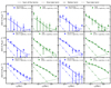 |
Fig. 1. Excess surface density (ESD) from the DECaLS shear catalog and the corresponding best fitting results. The symbols in the 12 panels show the ESD profiles obtained by stacking the lensing signals for galaxies in each stellar mass bin, as indicated in each panel. Results are shown separately for star-forming galaxies (first and third columns) and the total population (second and fourth columns). The error bars correspond to the standard deviation of 150 bootstrap samples. We fit the ESD by using three components, the stellar mass term (dotted lines with stars), the one-halo term (dashed lines), and the two-halo term (dash-dotted lines). The sum of these components are shown with solid lines. |
Following previous studies (e.g., Mandelbaum et al. 2008; Leauthaud et al. 2010; Luo et al. 2018), we modeled the ESD using three components:
 (2)
(2)
The first term is the contribution of the stellar mass of galaxies. We adopted the stellar mass directly from the observational data and modeled it as a point mass. The second term is the contribution of the dark matter halo, assumed to have a Navarro–Frenk–White (NFW; Navarro et al. 1997) density profile, described by two free parameters: the mass mh and the concentration c. Specifically, mh is the mass contained in a spherical region of radius r200m, within which the mean mass density is equal to 200 times the mean matter density of the Universe. The distributions of the halo mass and concentration for a fixed galaxy stellar mass are usually quite broad. In our modeling, we used a single NFW profile with two free parameters, mh and concentration, to fit the data point, ignoring the dispersion in them. Since our analysis focuses only on the average information of halos, the bias produced by ignoring the dispersion is expected to be small, as shown in Mandelbaum et al. (2016) and discussed further in Sect. 3.3. Following Mandelbaum et al. (2016), we also ignored the effect of off-centering, which is negligible for the mh estimation of central galaxies according to our tests. The third term, referred to as the two-halo term, was calculated by projecting the halo-matter cross-correlation function, ξhm, along the line of sight. Here ξhm = b(mh)ξmm, with ξmm being the linear matter–matter correlation function and b(mh) the linear halo bias (Tinker et al. 2010), both generated using COsmology, haLO and large-Scale StrUcture toolS (COLOSSUS Diemer 2018). We sampled the posterior distribution of the two parameters, mh and c, using the Monte Carlo Markov chain (MCMC) provided by the public open software emcee (Foreman-Mackey et al. 2013). Both COLOSSUS and emcee are under the MIT License. The best fitting profiles are presented in Fig. 1. The quoted mass, mh, is the median value of the posterior, and its error bar indicates the 16 and 84% range of the posterior.
We note that mh accounts for the contribution from cold dark matter, diffuse gas, and satellites around centrals, but does not include the contribution from the central galaxies that is modeled by ΔΣstellar. The total mass of the halo, which is used to calculate the conversion efficiency in the following and should include all the components within the virial radius of the halo, is thus Mh = mh + M*. In general, M* ≪ mh, and so Mh is very close to mh. However, for halos with very high efficiency, central galaxies can also make a significant contribution to the total halo mass. In the rest of the paper, halo mass refers to the total mass of the halo, Mh.
2.3. Weak lensing calibrated satellite kinematics method
The kinematics of satellite galaxies provides an important probe of the gravitational potential wells of the dark matter halos (e.g., McKay et al. 2002; van den Bosch et al. 2004; More et al. 2011; Wojtak & Mamon 2013; Lange et al. 2019a,b; Abdullah et al. 2020; Seo et al. 2020). For a central galaxy of mass M* in a given subsample, we identified its satellite candidates from a reference galaxy sample. For our analysis, we define the reference sample as a magnitude-limited sample following the following selection criteria: r-band Petrosian apparent magnitude of r < 17.6, r-band Petrosian absolute magnitude in the range ( − 24, −16), and redshift in the range 0.01 < z < 0.2 (Wang & Li 2019; Zhang et al. 2021). The candidates were defined as those that satisfy the following criteria: |Δv|≤3vvir, rp ≤ rvir, and Ms < M*. Here: rp and Δv are the projected distance and the line-of-sight velocity difference between the central in question and its satellite, respectively; rvir and vvir are, respectively, the virial radius and virial velocity calculated using the mean halo mass of the subsample derived from weak lensing; and Ms is the stellar mass of the satellite. The numbers of satellite candidates for different central galaxy samples are listed in Table 1.
Figure 2 shows the PDFs of Δv for the selected satellites associated with different (total and star-forming) central galaxy subsamples. We used a Gaussian plus a constant,
 (3)
(3)
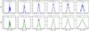 |
Fig. 2. Distribution of the line-of-sight velocity difference (Δv) between central galaxies and their satellite candidates. The solid lines with error bars show the PDF of Δv. The dashed lines show the Gaussian-plus-a-constant fits to the data points. The error bars correspond to the standard deviation of 100 bootstrap samples. The upper row shows the results for star-forming centrals, while the lower row is for the total central population. The results of the star-forming and total samples in different stellar mass bins are shown in different columns. We note that the scales of the vertical axes are different for different panels. |
to fit the PDFs. Here, the Gaussian component represents the true satellites, and the constant component is used to account for the interlopers that are not physically associated with the centrals (see also McKay et al. 2002; Brainerd & Specian 2003; van den Bosch et al. 2004; Conroy et al. 2007). An MCMC technique was used to perform the fitting. As can be seen from the figure, the Δv distributions are well fitted by the two-component model, and the contribution of the interlopers is negligible. Given that the uncertainty of an SDSS galaxy redshift is about 35 km s−1, the error of Δv is  km s−1. So, the velocity dispersion, σs, of satellites can be estimated from the best fitting Gaussian after correcting for the redshift uncertainties,
  . The estimate of σs may be affected by the uncertainty of the halo masses that are used to determine rvir and vvir. As a check, for each sample we compared the σs calculated using three different halo masses, corresponding to the 16%, 50%, and 84% of the posterior distribution obtained from the MCMC fitting to the stacked lensing profiles of the sample in question. We find that the three values of σs so obtained are in general consistent with one another (see Appendix A for details). We thus conclude that the uncertainty in the halo mass has little impact on the estimate of σs.
In Fig. 3 we show σs vs. Mh, the lensing mass measurement, for both the total and star-forming samples. One can see a strong correlation between the two parameters. We fit the data points for the total sample with a power-law model, and the constrained relation is
 (4)
(4)
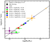 |
Fig. 3. Halo mass–satellite velocity dispersion relation. The open (solid) diamonds show the velocity dispersion (σs) of satellites versus the host halo masses for total (star-forming) central galaxies. The halo masses are measured from DECaLS lensing data. Different colors indicate different stellar mass bins of central galaxies. The error bars for halo mass indicate the 16% and 84% of the posterior distribution obtained from the MCMC fitting to the stacked lensing profiles. The error bars for σs represent the 16% and 84% of the posterior distribution obtained from the fitting to the distribution of the satellite-central velocity difference. The solid line represents the best fit to the data points for the total galaxy sample. |
Remarkably, the slope of the relation is in excellent agreement with what is expected from the virial scaling relation (M ∝ σ3) seen in numerical simulations (Evrard et al. 2008). A similar slope has been obtained in previous studies that measured halo mass using abundance matching, satellite kinematics, the caustic technique, the SZ effect, and the virial theorem (e.g., Yang et al. 2007; More et al. 2011; Rines et al. 2013, 2016; Abdullah et al. 2020), although some other studies find different results (e.g., Viola et al. 2015). Our tests show that both weak lensing and satellite kinematics can provide robust and consistent measurements of the host halo masses of galaxies. The star-forming galaxies also closely follow the trend defined by the total sample, demonstrating that the lensing masses for star-forming galaxies are also robust.
Thus, we can derive the host halo masses for the star-forming and total subsamples from their measured σs (Fig. 2) using the σs − Mh relation. But, since σs is also used in fitting the relation, the uncertainties in σs and in the relation are expected to be correlated. In order to avoid this correlation, we designed a new way to calculate the σs − Mh relation. Specifically, for each stellar mass bin, we only used data points (σs vs. Mh) in the rest of the stellar mass bins to fit the σs − Mh relation so that the derived relation is independent of the galaxy sample in question. In Appendix B we show the best fitting σs − Mh relations for all six stellar mass bins.
We then combined the σs of galaxy sample with its corresponding σs − Mh relation to derive the halo mass. The errors of the halo masses were obtained by considering both the uncertainties in σs and the Mh − σs relation. Both σs and the Mh − σs relation were derived using MCMC fitting, which can provide their posterior distributions. For galaxies in a given stellar mass bin, we can randomly generate a σs value and a Mh − σs relation from their posterior distributions and predict a halo mass by combining the two. In practice, we generated 30 000 predictions of the halo mass for each subsample and used the 16% and 84% of the mass distribution to represent the uncertainties. The halo mass estimated in this way is referred to as the weak lensing calibrated satellite kinematics (LcSK) halo mass and is also denoted by Mh.
Finally, we want to note that the uncertainties of the LcSK masses in different stellar mass bins are correlated. Therefore, if one wants to use these data points to constrain a galaxy formation model, one should consider the covariance among different stellar mass bins.
2.4. Galaxy clustering analysis
Galaxy clustering can be used to measure the large-scale environment and to infer the halo mass for a sample of selected galaxies. In this paper we adopt the projected two-point cross-correlation function (2PCCF) to quantify the clustering of galaxies. We first estimated the 2PCCF using
 (5)
(5)
where NR and ND are the galaxy numbers in the random and reference samples, respectively; rp and rπ are the separations perpendicular and parallel to the line of sight, respectively; GD is the number of cross pairs between the selected galaxy sample and the reference sample; and GR is that between the selected galaxy sample and the random sample. To obtain the projected 2PCCF, we integrated ξ along the line of sight,  , with Δs = 40 h−1 Mpc, which is sufficiently large so as to include almost all correlated pairs. The errors on the measurements of the 2PCCF were estimated by using 100 bootstrap samples.
The reference sample used here is the same as that described in Sect. 2.3. Based on this reference sample, we constructed a random sample in the following way (see also Li et al. 2006, for more details). We generated ten duplicates for each galaxy in the reference sample and randomly placed them in the SDSS sky coverage. All other properties, including the stellar mass and redshift of the duplicate galaxies, are the same as those of the original galaxy. Thus, the random sample has the same survey geometry and the same distribution of galaxy properties as the reference sample.
The 2PCCFs of the star-forming galaxy sample cannot be directly compared with those of the total galaxy sample, because the two samples may have different redshift distributions. In order to make a fair comparison, it was necessary to construct a control sample that matches the star-forming sample. For a star-forming galaxy in a given stellar mass bin, we selected, from the total galaxy subsample in the same stellar mass bin, n galaxies whose redshift are within 0.005 of the star-forming galaxy in question. We chose n = [1, 1, 1, 2, 4, 19] for the six galaxy stellar mass bins (see Sect. 2). The number of control galaxies, n, was chosen according to the ratio in size between the total and star-forming galaxy subsamples. This control sample was then used to estimate the 2PCCFs to compare with the corresponding star-forming galaxies.
3. Results
3.1. The stellar mass–halo mass relation
Figure 4 and Table 1 show the halo mass (Mh) obtained from weak lensing (lensing mass) and from the LcSK method, separately for the total and star-forming central galaxies of different stellar masses. Both estimates give very similar results, as is expected from the tight correlation between the velocity dispersion and the lensing mass (Fig. 3). For comparison, we also show the results in the literature obtained using various methods, including galaxy groups, abundance matching, the conditional luminosity function, weak lensing, and the empirical model (Yang et al. 2009; Moster et al. 2010; Leauthaud et al. 2012; Kravtsov et al. 2018; Behroozi et al. 2019). As one can see from the figure, the SHMR for our total galaxy sample closely follows the trend defined by previous results. In contrast, for a given stellar mass, the halo mass of star-forming galaxies is lower than that of the total sample, and the difference becomes larger and more significant at the high-mass end. This is broadly consistent with previous weak-lensing and satellite kinematics studies that find that star-forming or blue galaxies reside in less massive halos than quiescent or red galaxies of the same stellar mass (see, e.g., Mandelbaum et al. 2006, 2016; More et al. 2011; Lange et al. 2019b; Zhang et al. 2021) as well as with results obtained from some empirical models constrained by observational data (e.g., Rodríguez-Puebla et al. 2015; Behroozi et al. 2019).
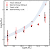 |
Fig. 4. Stellar mass–halo mass relation. The red symbols with error bars show the SHMR calculated using the halo mass obtained from the fits to the stacked lensing mass profiles from the DECaLS shear catalog, while the black ones are based on the LcSK method. For clarity, we shift the black symbols slightly toward the left. The error bars reflect the 16% and 84% of the posterior distribution. The diamonds and squares show the results for star-forming and total populations, respectively. The shadow region represents the range covered by curves published in Yang et al. (2009), Moster et al. (2010), Leauthaud et al. (2012), Kravtsov et al. (2018), and Behroozi et al. (2019). |
3.2. The conversion efficiency
Assuming that the baryon fraction within halos is equal to the cosmic fraction (fb), the overall conversion efficiency can be represented by M*/(fbMh). Here Mh is the total mass of a dark matter halo and M* is the stellar mass of the central galaxy within the halo. In the left panel of Fig. 5, we show this conversion efficiency as a function of stellar mass for the total galaxy sample, with the halo mass measured directly from the weak lensing data. The efficiency for the total galaxy sample peaks roughly at M* ∼ 1010.6 M⊙ and decreases toward both lower- and higher-mass ends, in good agreement with previous results (e.g., Wechsler & Tinker 2018). The same panel also shows the results for the star-forming central galaxies defined in Sect. 2. The efficiency of star-forming galaxies roughly follows the trend of the total population at the low-mass end but deviates from it and continues the increasing trend toward the massive end. For star-forming galaxies of M* ∼ 1011 M⊙, the efficiency reaches a value of  , much higher than the maximum value of ∼0.2 for Milky-Way-like galaxies with M* ∼ 1010.6 M⊙. At M* > 1011 M⊙, the high efficiency seems to remain, although with a larger uncertainty. This high efficiency indicates that most of the baryonic gas in the host halos of those massive star-forming galaxies has already assembled into galaxies and been converted into stars.
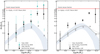 |
Fig. 5. Baryon conversion efficiency as a function of stellar mass. In the left panel, the symbols with error bars show the efficiency calculated using the halo mass obtained from the fits to the stacked lensing mass profiles. The black symbols show the results from the DECaLS shear catalog, while the green ones are obtained from the SDSS shear catalog (see Appendix C). The solid and open symbols show the results for the star-forming and total populations, respectively. Error bars indicate the 16% and 84% of the posterior distribution obtained from the MCMC fitting. In the right panel, the symbols with error bars show the efficiency calculated using the LcSK method. The error bars reflect the 16% and 84% of the posterior distribution obtained from the LcSK. The solid (dashed) gray lines show the results for star-forming (total) galaxies in the hydro-simulation IllustrisTNG. The shadow region in the two panels covers the range obtained before, as in Fig. 4. |
We can also use the halo mass obtained from the LcSK method to estimate the conversion efficiency (Sect. 2.3), and the results are presented in the right panel of Fig. 5 and in Table 1. The results are very similar to those obtained from the weak lensing data. For example, the efficiency for the second most massive star-forming sample is  . However, the LcSK method significantly reduces the uncertainty of the efficiency in most of the stellar mass bins.
As mentioned above, many previous studies have found that star-forming or blue galaxies tend to reside in smaller halos than quenched or red galaxies of the same stellar mass (e.g., More et al. 2011; Hudson et al. 2015; Mandelbaum et al. 2016; Lange et al. 2019b; Behroozi et al. 2019; Posti et al. 2019; Bilicki et al. 2021). This is consistent with our results that the conversion efficiency is higher for star-forming galaxies than for quenched galaxies. However, in comparison with our results, the implied conversion efficiency is significantly lower and has larger uncertainties in many of the earlier studies. For example, Mandelbaum et al. (2006, 2016) find a peak efficiency of  for late-type galaxies and
  for blue galaxies, respectively. Dutton et al. (2011) find that the mean peak efficiency for their late-type galaxies is around 0.3. Rodríguez-Puebla et al. (2015) find that the M*-to-Mh ratio of their blue centrals has a peak value of 0.051, corresponding to a conversion efficiency of 0.325 assuming fb = 0.157. These results appear to be in conflict with ours, and we will come back to this issue later. Recently, Posti et al. (2019) modeled the rotation curves of local disk galaxies and inferred the halo mass of individual galaxies. They find that the mean conversion efficiency for about 20 massive disk galaxies is about 0.5, albeit with large uncertainties. Our results are in broad agreement with theirs. However, our results were obtained from a large sample of 22 099 star-forming galaxies, indicating that the high conversion efficiency is a common property for massive star-forming galaxies.
3.3. Tests of uncertainties
A number of factors may affect the estimates of the halo mass. As a test, we repeated our analysis using an independent weak-lensing shear catalog obtained by Luo et al. (2017) from SDSS DR7 (Abazajian et al. 2009) imaging data using a totally different method (see Appendix C). As shown in Fig. 5, the results obtained from the SDSS data agree well with those from the DECaLS data. However, the SDSS results have much larger uncertainties because of the shallower imaging data used to measure the weak lensing shear.
Galaxy clustering provides another test because of its dependence on halo mass (Mo & White 1996; Tinker et al. 2010). Figure 6 shows the ratio of the 2PCCF, in the range 5 Mpc < rp < 20 Mpc, between star-forming galaxies and the total population in four high-mass bins (see Sect. 2.4 for the method for estimating the 2PCCF). In each panel the theoretical prediction using the linear halo bias model (Tinker et al. 2010) is shown, and the halo mass was derived from the DECaLS weak lensing measurements. As one can see, the model predictions agree very well with the observational results on large scales, where the linear halo bias model is valid. However, halo bias may also depend on the halo assembly history, in addition to halo mass (e.g., Gao et al. 2005; Wang et al. 2007). If there is a correlation between the properties of the central galaxy in a halo and the assembly of the halo, then the halo bias model used here may not be an accurate description of star-forming and quenched centrals. Unfortunately, this potential correlation is not understood well enough to quantify the effect it may have on our results.
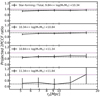 |
Fig. 6. Ratio of the 2PCCF between star-forming galaxies and the total control galaxies as a function of the projected distance (rp) in different stellar mass bins. Error bars are the standard deviation of the 2PCCF ratio among 100 bootstrap samples. The horizontal dashed line in each panel indicates the theoretical ratio from a halo bias model (Tinker et al. 2010) that uses the halo mass measured from weak lensing as the input. For clarity, we only show the results for the four highest-mass bins, where the uncertainties in lensing mass measurements are relatively small. |
As discussed above, the conversion efficiency obtained here for massive star-forming galaxies appears to be higher than that obtained in some previous investigations. One cause of the discrepancy may be that galaxy samples used in these investigations are different from ours. For example, Mandelbaum et al. (2016) and Bilicki et al. (2021) split galaxy samples according to galaxy color, instead of the SFR used here. As a test, we repeated our analysis by separating red and blue galaxies according to Eq. (1) in van den Bosch et al. (2008), similarly to how it was done in Mandelbaum et al. (2016). The SHMRs obtained from the red and blue populations are shown in Fig. 7, in comparison with the results taken from Table B1 of Mandelbaum et al. (2016)5 and from Bilicki et al. (2021). As one can see, our results are in good agreement with theirs, which provides additional support to the reliability of our mass estimates. In particular, blue galaxies of M* ∼ 1011 M⊙ have an average halo mass of  from Mandelbaum et al. (2016) and
  from Bilicki et al. (2021), corresponding to a conversion efficiency of
  and
and  , respectively, much lower than that for star-forming galaxies of the same stellar mass (Fig. 5 and Table 1). This suggests that the calculated efficiencies are sensitive to the sample selection, and that the discrepancy between our results (samples selected according to the SFR) and their results (samples selected according to galaxy colors) is entirely due to the difference in the sample selection.
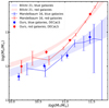 |
Fig. 7. Comparison of our SHMR with those of Mandelbaum et al. (2016) and Bilicki et al. (2021). The diamonds, the lines with error bars, and the shaded regions are the SHMRs from our results, Mandelbaum et al. (2016), and Bilicki et al. (2021), respectively. The solid symbols show the results calculated using the DECaLS shear catalog. The red and blue represent the red and blue galaxy samples, respectively. |
Other potential problems may also exist in the halo mass estimation. If a fraction of the selected galaxies are satellites, instead of centrals, a systematic bias can be introduced, as our modeling of the lensing measurements assumes that all galaxies are centrals. Contamination by satellites is expected to lead to an overestimation of the halo mass (Mandelbaum et al. 2006, 2016), and so the conversion efficiency may be underestimated in our results. To check the impact of this effect, we conducted an analysis by using an additional selection criterion to reduce the contamination of satellites in our central galaxy samples. Specifically, we required that a central galaxy be the most massive one among all its neighbors that have projected distances of less than 1 Mpc and line-of-sight velocity differences smaller than 1000 km s−1 relative to the galaxy in question. This leads to a sample of 4900 star-forming galaxies in the second most massive bin. The halo mass obtained from lensing for this sample is  , very close to the value obtained above, demonstrating that the effect of satellite contamination is negligible in our results.
Another bias in the halo mass estimate may arise because halos of galaxies in a given sample can span a large range in mass. The stacked lensing signal around the sample galaxies is, therefore, an average of many different halo profiles, and using a single NFW profile to fit the average profile may introduce a bias. Detailed tests by Mandelbaum et al. (2016) using a mock catalog constructed from a semi-analytic galaxy formation model suggest that the best fitting mass underestimates the mean halo mass by about 10%, quite independent of the stellar mass and galaxy color. At M* ∼ 1011 M⊙, the actual mean halo mass may be about 1.14 times the best fitting halo mass. Taking this correction into account, the conversion efficiency for star-forming galaxies in this mass range changes to 0.629/1.14 = 0.552. One should keep in mind that the correction factor may depend on the used galaxy formation model. As we see below, our results are not well reproduced by the current galaxy formation models.
Yet another important source of uncertainty comes from the estimate of the stellar mass. The statistical uncertainty of the stellar mass is usually 0.3 dex (e.g., Kauffmann et al. 2003b). Our galaxy sample is large enough that the statistical error in the mean stellar mass is small. However, the systematic uncertainties, such as those produced by the adopted initial mass function, the star-formation history, the stellar library, and the dust attenuation, may not be negligible (see Moustakas et al. 2013, for a brief introduction). It is in general difficult to evaluate such systematic uncertainties within a specific model of the stellar population. One common practice is to perform a consistency check by comparing the stellar masses of the same object measured with different techniques and/or from different data. The MPA masses used here have been used in many comparison studies in the literature. For example, Moustakas et al. (2013) showed that the MPA masses are in excellent agreement with theirs based on the fits to SEDs in 12 UV, optical, and infrared bands. As a check, we made a similar comparison for central star-forming galaxies, as they are the most relevant to our results. In Fig. 8 we compare the MPA masses with those given in NYU-VAGC and those obtained by Salim et al. (2016). Different approaches and/or data were used to derive stellar masses in these three databases. As one can see, there are some systematic differences among the three masses. At M* ∼ 1011 M⊙, the difference between the MPA mass and the other two is about 0.05 dex, and the MPA mass appears to lie between the two masses. Thus, our results are robust as long as the systematic bias in the stellar mass is not much larger than the difference among the three mass estimates compared here.
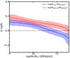 |
Fig. 8. Comparison of the MPA-JHU stellar mass with the stellar masses from NYU-VAGC (blue) and Salim et al. (2016) (red) for central star-forming galaxies. The solid lines show the median value of the residual, while the shaded regions show the 25% and 75% of the residual distribution. |
4. Discussion
One possible explanation for the large M*-to-Mh ratio reported here is that the host halos are splashback halos (e.g., Ludlow et al. 2009) that entered the virial radii of more massive halos at some point and were severely stripped by the tidal field. However, splashback halos are usually much more strongly clustered than other halos of the same mass (Wang et al. 2009) because they are spatially close to massive halos. This is clearly inconsistent with the fact that the massive star-forming galaxies are less clustered than the total population of the same mass (Fig. 6). Moreover, environmental effects may quench the star formation in splashback halos, and so their galaxies are not expected to be star forming. Thus, this possibility can be ruled out.
Another possibility is that some processes that are supposed to prevent the growth of massive galaxies did not operate on these galaxies in the past. Figure 9 shows the distributions of galaxy concentration for star-forming and total galaxies with M* ∼ 1011 M⊙. One can see that star-forming galaxies have much smaller concentrations than galaxies of the same mass from the total sample. The activities of AGNs, which are thought to be capable of quenching star formation, are expected to be more prominent in more concentrated galaxies (e.g., Kauffmann et al. 2003a; Zhang et al. 2021). Previous theoretical and observational studies have found that the efficiency of star-forming galaxies may be suppressed by several feedback processes, such as supernova and AGN feedback in the low and high stellar mass ends, respectively. Our results suggest that AGN feedback must be inefficient in suppressing cold gas acquisition and star formation in massive star-forming galaxies. Active galactic nucleus feedback may still be effective in quenching the star formation in other massive galaxies of M* ∼ 1011 M⊙ and may thus produce a much lower conversion efficiency in them. As shown in Table 1, the number of massive star-forming galaxies (M* ∼ 1011 M⊙) is much smaller than that of the total galaxy population of the same mass. Thus, this absence of effective AGN feedback only applies to a relatively small fraction of the total galaxy population.
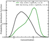 |
Fig. 9. Probability distributions of galaxy concentration (C = R90/R50) for the total galaxy sample (green line) and the massive star-forming galaxy sample (black line) of M* ∼ 1011 M⊙. |
These massive star-forming galaxies have already converted more than 60% of their halo gas into stars. Based on CO and HI observations, Saintonge et al. (2016) find that these galaxies on average contain about ∼1010 M⊙ in cold gas. Thus, the total baryon mass in these galaxies is more than 70% of the total baryons in their halos. This leaves less than 30% of the baryons in the circumgalactic medium (CGM). Thus, observations of the CGM may provide an independent way to check our results. The CGM can be probed in a number of ways, such as via quasar absorption line systems (e.g., Tumlinson et al. 2017), extended X-ray emission (e.g., Anderson et al. 2013), and the SZ effect (e.g., Lim et al. 2018). Many studies have found evidence for the existence of CGM in galaxies with a wide range of stellar mass (e.g., Tumlinson et al. 2017). However, a detailed comparison with our results is not straightforward. As shown in Table 1, star-forming galaxies of 1011 M⊙ make up only about one-fifth of the total population of the same mass. It is thus inappropriate to compare our results directly with those of studies that did not separate the star-forming galaxies from the total population. For low-ionization line systems observed in star-forming galaxies, such as MgII, the absorbing gas is believed to be associated with outflow (e.g., Lan & Mo 2018). The total amount of gas involved may not be large, which is consistent with our results.
The mean density of the CGM around massive star-forming galaxies is expected to be less than that around other galaxies. Therefore, the timescale for gas cooling, which is inversely proportional to the gas density, is much longer. The ability of massive star-forming galaxies to acquire additional gas to maintain a high SFR should be significantly suppressed. Our results suggest that the well-known flattening of the SFR–M* relation for star-forming galaxies at the massive end (Whitaker et al. 2014; Saintonge et al. 2017) is caused by the decrease in gas supply. It is consistent with the analysis based on atomic and molecular gas within galaxies (Saintonge et al. 2016).
The high galaxy-to-halo mass ratio for massive star-forming galaxies may have important implications for their rotation curves. To demonstrate this, we selected galaxies with M* ∼ 1011 M⊙ and a Sèrsic index of n ∼ 1 from the SDSS galaxy sample. These massive disk galaxies have a wide distribution of Sèrsic r0 (which is equal to the disk scale length for n = 1), ranging from 2.5 to 6.3 kpc, where both n and r0 are taken from the NYU-VAGC catalog (Blanton et al. 2005a). To derive the rotation curve, we assumed an exponential mass profile with a typical disk scale length of 4.4 Kpc for a massive disk galaxy and an NFW profile for its host dark matter halo. In Fig. 10 we show the rotation curve for a halo mass of Mh = 1012 M⊙ (with concentration c = 13), about the average value for star-forming galaxies with M* ∼ 1011 M⊙. For comparison, we also show the rotation curve for a disk galaxy residing in a halo of 1012.6 M⊙ (c = 11), as expected from our total galaxy sample with M* ∼ 1011 M⊙ (see Fig. 4). For Mh = 1012.6 M⊙, the predicted rotation curve is quite flat at large radii, as is observed for many disk galaxies. In contrast, for Mh = 1012 M⊙, the rotation curve reaches a peak at ∼10 kpc and gradually decreases at larger radii. This type of rotation curve is not common for the general disk population but has been found for some local galaxies (e.g., Corbelli et al. 2010; Posti et al. 2019). Modeling their rotation curves shows that these galaxies indeed have a high conversion efficiency (Posti et al. 2019). Our results show that this type of rotation curve should be expected for massive star-forming disks.
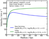 |
Fig. 10. Rotation curves for two disk galaxies with a stellar mass of 1011 M⊙ but with a halo mass of 1012 M⊙ (star-forming, blue) and 1012.6 M⊙ (total, green). The two disk galaxies have the same stellar mass exponential profiles, with a disk scale length of 4.4 kpc and a Sèrsic index of n = 1. Dark matter halos are assumed to have an NFW profile with the concentration-mass relation from Zhao et al. (2009); c = 13 for the blue line, and c = 11 for the green line. |
Finally, we examined whether current galaxy formation models can reproduce our results. In the right panel of Fig. 5, we show the results obtained from the Illustris-TNG simulation (Pillepich et al. 2018), which implements a series of baryonic physics, such as AGN feedback, to suppress star formation in massive galaxies (see Appendix D for a brief description of the simulation). As can be seen from the figure, the simulation result for the total sample has a peak around a stellar mass between 1010.5 and 1011 M⊙, consistent with the observational results. However, the simulation fails to reproduce the high conversion efficiency for the observed massive star-forming galaxies. Indeed, massive star-forming galaxies in the simulation closely follow the total population over almost the entire stellar mass range. It is likely that the AGN feedback implemented in the simulation is too strong for these galaxies. We also examined the Eagle simulation (Schaye et al. 2015) and find that it cannot reproduce the high conversion efficiency observed for massive star-forming galaxies either. Thus, our finding presents a challenging problem for current simulations in their modeling of feedback and star formation.
5. Summary
Based on the shear catalog of DECaLS imaging data, we have derived the halo mass of central galaxies selected from the SDSS. We have developed an LcSK method to improve the halo mass measurements. We then obtained the efficiency for converting baryons into stars within halos, defined as M*/Mh/fb, for both the total galaxy population and galaxies in the star-forming main sequence. Our main results are summarized as follows.
-
The SHMR for the total galaxy population we obtained is in good agreement with previous studies. The conversion efficiency peaks around Milky-Way-like galaxies and declines toward both lower and higher stellar mass ends.
-
The conversion efficiency of star-forming galaxies increases monotonically with stellar mass and reaches a value of more than 60 percent at M∗ ∼ > 1011 M⊙. Thus, these galaxies have converted most of their halo gas into stars.
-
Our tests show that the measurements of the halo mass are consistent with the results obtained from the SDSS shear catalog and from galaxy clustering.
-
Massive star-forming galaxies are expected to have rotation curves that are peaked at about two disk scale lengths and decline at larger distances, quite different from the flat rotation curves commonly observed for the general disk population.
-
The high conversion efficiency observed for massive star-forming galaxies is not reproduced by current cosmological gas simulations.
-
We have tested a number of systematic effects that may affect our results and find that none of them can change our conclusions significantly.
Our finding has important implications for the understanding of galaxy formation and star-formation quenching. The high conversion efficiency observed for massive star-forming galaxies indicates that AGN feedback may not have had an important effect on the conversion of gas into stars in these particular galaxies. The fact that current cosmological hydrodynamic simulations cannot reproduce such a high conversion efficiency indicates that our current understanding of feedback is still incomplete, at least for massive star-forming galaxies. Clearly, the observational results presented here provide an important constraint on modeling feedback processes in galaxy formation, and we will come back to this in a future paper.
The galaxy group catalog is publicly available at https://gax.sjtu.edu.cn/data/Group.html
The galaxy size data can be downloaded at http://sdss.physics.nyu.edu/vagc/
The DECaLS shear catalog is publicly available at https://gax.sjtu.edu.cn/data/DESI.html
To be consistent, the stellar masses are adopted from the MPA-JHU catalog, and their halo masses are uncorrected; see the paper for the correction.
Acknowledgments
We thank the referee for useful comments. This work is supported by the National Key R&D Program of China (grant No. 2018YFA0404503; grant No. 2018YFA0404504), the National Natural Science Foundation of China (NSFC, Nos. 11733004, 12192224, 11890693, 11421303, 11890691, 11621303, 11833005 and 11890692), and the Fundamental Research Funds for the Central Universities. The authors gratefully acknowledge the support of Cyrus Chun Ying Tang Foundations. We acknowledge the science research grants from the China Manned Space Project with No. CMS-CSST-2021-A03. The work is also supported by the Supercomputer Center of University of Science and Technology of China. The Legacy Surveys consist of three individual and complementary projects: the Dark Energy Camera Legacy Survey (DECaLS; Proposal ID #2014B-0404; PIs: David Schlegel and Arjun Dey), the Beijing-Arizona Sky Survey (BASS; NOAO Prop. ID #2015A-0801; PIs: Zhou Xu and Xiaohui Fan), and the Mayall z-band Legacy Survey (MzLS; Prop. ID #2016A-0453; PI: Arjun Dey). DECaLS, BASS and MzLS together include data obtained, respectively, at the Blanco telescope, Cerro Tololo Inter-American Observatory, NSF’s NOIRLab; the Bok telescope, Steward Observatory, University of Arizona; and the Mayall telescope, Kitt Peak National Observatory, NOIRLab. The Legacy Surveys project is honored to be permitted to conduct astronomical research on Iolkam Du’ag (Kitt Peak), a mountain with particular significance to the Tohono O’odham Nation. NOIRLab is operated by the Association of Universities for Research in Astronomy (AURA) under a cooperative agreement with the National Science Foundation. This project used data obtained with the Dark Energy Camera (DECam), which was constructed by the Dark Energy Survey (DES) collaboration. Funding for the DES Projects has been provided by the US Department of Energy, the US National Science Foundation, the Ministry of Science and Education of Spain, the Science and Technology Facilities Council of the United Kingdom, the Higher Education Funding Council for England, the National Center for Supercomputing Applications at the University of Illinois at Urbana-Champaign, the Kavli Institute of Cosmological Physics at the University of Chicago, Center for Cosmology and Astro-Particle Physics at the Ohio State University, the Mitchell Institute for Fundamental Physics and Astronomy at Texas A&M University, Financiadora de Estudos e Projetos, Fundacao Carlos Chagas Filho de Amparo, Financiadora de Estudos e Projetos, Fundacao Carlos Chagas Filho de Amparo a Pesquisa do Estado do Rio de Janeiro, Conselho Nacional de Desenvolvimento Cientifico e Tecnologico and the Ministerio da Ciencia, Tecnologia e Inovacao, the Deutsche Forschungsgemeinschaft and the Collaborating Institutions in the Dark Energy Survey. The Collaborating Institutions are Argonne National Laboratory, the University of California at Santa Cruz, the University of Cambridge, Centro de Investigaciones Energeticas, Medioambientales y Tecnologicas-Madrid, the University of Chicago, University College London, the DES-Brazil Consortium, the University of Edinburgh, the Eidgenossische Technische Hochschule (ETH) Zurich, Fermi National Accelerator Laboratory, the University of Illinois at Urbana-Champaign, the Institut de Ciencies de l’Espai (IEEC/CSIC), the Institut de Fisica d’Altes Energies, Lawrence Berkeley National Laboratory, the Ludwig Maximilians Universitat Munchen and the associated Excellence Cluster Universe, the University of Michigan, NSF’s NOIRLab, the University of Nottingham, the Ohio State University, the University of Pennsylvania, the University of Portsmouth, SLAC National Accelerator Laboratory, Stanford University, the University of Sussex, and Texas A&M University. BASS is a key project of the Telescope Access Program (TAP), which has been funded by the National Astronomical Observatories of China, the Chinese Academy of Sciences (the Strategic Priority Research Program “The Emergence of Cosmological Structures” Grant # XDB09000000), and the Special Fund for Astronomy from the Ministry of Finance. The BASS is also supported by the External Cooperation Program of Chinese Academy of Sciences (Grant # 114A11KYSB20160057), and Chinese National Natural Science Foundation (Grant # 11433005). The Legacy Survey team makes use of data products from the Near-Earth Object Wide-field Infrared Survey Explorer (NEOWISE), which is a project of the Jet Propulsion Laboratory/California Institute of Technology. NEOWISE is funded by the National Aeronautics and Space Administration. The Legacy Surveys imaging of the DESI footprint is supported by the Director, Office of Science, Office of High Energy Physics of the US Department of Energy under Contract No. DE-AC02-05CH1123, by the National Energy Research Scientific Computing Center, a DOE Office of Science User Facility under the same contract; and by the US National Science Foundation, Division of Astronomical Sciences under Contract No. AST-0950945 to NOAO. The Photometric Redshifts for the Legacy Surveys (PRLS) catalog used in this paper was produced thanks to funding from the US Department of Energy Office of Science, Office of High Energy Physics via grant DE-SC0007914.
References
- Abazajian, K. N., Adelman-McCarthy, J. K., Agüeros, M. A., et al. 2009, ApJS, 182, 543 [Google Scholar]
- Abdullah, M. H., Wilson, G., Klypin, A., et al. 2020, ApJS, 246, 2 [Google Scholar]
- Anderson, M. E., Bregman, J. N., & Dai, X. 2013, ApJ, 762, 106 [NASA ADS] [CrossRef] [Google Scholar]
- Barrow, J. D., Bhavsar, S. P., & Sonoda, D. H. 1984, MNRAS, 210, 19 [Google Scholar]
- Behroozi, P., Wechsler, R. H., Hearin, A. P., & Conroy, C. 2019, MNRAS, 488, 3143 [NASA ADS] [CrossRef] [Google Scholar]
- Bilicki, M., Dvornik, A., Hoekstra, H., et al. 2021, A&A, 653, A82 [NASA ADS] [CrossRef] [EDP Sciences] [Google Scholar]
- Blanton, M. R., Eisenstein, D., Hogg, D. W., Schlegel, D. J., & Brinkmann, J. 2005a, ApJ, 629, 143 [Google Scholar]
- Blanton, M. R., Schlegel, D. J., Strauss, M. A., et al. 2005b, AJ, 129, 2562 [NASA ADS] [CrossRef] [Google Scholar]
- Bluck, A. F. L., Mendel, J. T., Ellison, S. L., et al. 2016, MNRAS, 462, 2559 [Google Scholar]
- Brainerd, T. G., & Specian, M. A. 2003, ApJ, 593, L7 [NASA ADS] [CrossRef] [Google Scholar]
- Bregman, J. N. 2007, ARA&A, 45, 221 [Google Scholar]
- Breiman, L. 2001, Mach. Learn., 45, 5 [Google Scholar]
- Brinchmann, J., Charlot, S., White, S. D. M., et al. 2004, MNRAS, 351, 1151 [Google Scholar]
- Cole, S., Lacey, C. G., Baugh, C. M., & Frenk, C. S. 2000, MNRAS, 319, 168 [Google Scholar]
- Conroy, C., Prada, F., Newman, J. A., et al. 2007, ApJ, 654, 153 [Google Scholar]
- Corbelli, E., Lorenzoni, S., Walterbos, R., Braun, R., & Thilker, D. 2010, A&A, 511, A89 [NASA ADS] [CrossRef] [EDP Sciences] [Google Scholar]
- Croton, D. J., Springel, V., White, S. D. M., et al. 2006, MNRAS, 365, 11 [Google Scholar]
- Dekel, A., & Birnboim, Y. 2006, MNRAS, 368, 2 [NASA ADS] [CrossRef] [Google Scholar]
- Dey, A., Schlegel, D. J., Lang, D., et al. 2019, AJ, 157, 168 [Google Scholar]
- Diemer, B. 2018, ApJS, 239, 35 [NASA ADS] [CrossRef] [Google Scholar]
- Dutton, A. A., Conroy, C., van den Bosch, F. C., et al. 2011, MNRAS, 416, 322 [NASA ADS] [Google Scholar]
- Evrard, A. E., Bialek, J., Busha, M., et al. 2008, ApJ, 672, 122 [Google Scholar]
- Fabian, A. C. 2012, ARA&A, 50, 455 [Google Scholar]
- Fall, S. M., & Efstathiou, G. 1980, MNRAS, 193, 189 [NASA ADS] [CrossRef] [Google Scholar]
- Foreman-Mackey, D., Hogg, D. W., Lang, D., & Goodman, J. 2013, PASP, 125, 306 [Google Scholar]
- Gao, L., Springel, V., & White, S. D. M. 2005, MNRAS, 363, L66 [NASA ADS] [CrossRef] [Google Scholar]
- Heckman, T. M., & Best, P. N. 2014, ARA&A, 52, 589 [Google Scholar]
- Hudson, M. J., Gillis, B. R., Coupon, J., et al. 2015, MNRAS, 447, 298 [Google Scholar]
- Kauffmann, G., & Charlot, S. 1998, MNRAS, 294, 705 [NASA ADS] [CrossRef] [Google Scholar]
- Kauffmann, G., Heckman, T. M., Tremonti, C., et al. 2003a, MNRAS, 346, 1055 [Google Scholar]
- Kauffmann, G., Heckman, T. M., White, S. D. M., et al. 2003b, MNRAS, 341, 33 [Google Scholar]
- Kravtsov, A. V., Vikhlinin, A. A., & Meshcheryakov, A. V. 2018, Astron. Lett., 44, 8 [Google Scholar]
- Kurczynski, P., Gawiser, E., Acquaviva, V., et al. 2016, ApJ, 820, L1 [NASA ADS] [CrossRef] [Google Scholar]
- Lan, T.-W., & Mo, H. 2018, ApJ, 866, 36 [NASA ADS] [CrossRef] [Google Scholar]
- Lange, J. U., van den Bosch, F. C., Zentner, A. R., Wang, K., & Villarreal, A. S. 2019a, MNRAS, 482, 4824 [NASA ADS] [CrossRef] [Google Scholar]
- Lange, J. U., van den Bosch, F. C., Zentner, A. R., Wang, K., & Villarreal, A. S. 2019b, MNRAS, 487, 3112 [Google Scholar]
- Leauthaud, A., Finoguenov, A., Kneib, J.-P., et al. 2010, ApJ, 709, 97 [Google Scholar]
- Leauthaud, A., Tinker, J., Bundy, K., et al. 2012, ApJ, 744, 159 [Google Scholar]
- Li, C., Kauffmann, G., Jing, Y. P., et al. 2006, MNRAS, 368, 21 [NASA ADS] [CrossRef] [Google Scholar]
- Lim, S. H., Mo, H. J., Li, R., et al. 2018, ApJ, 854, 181 [NASA ADS] [CrossRef] [Google Scholar]
- Lu, Z., Mo, H. J., Lu, Y., et al. 2014, MNRAS, 439, 1294 [NASA ADS] [CrossRef] [Google Scholar]
- Lu, Z., Mo, H. J., Lu, Y., et al. 2015, MNRAS, 450, 1604 [NASA ADS] [CrossRef] [Google Scholar]
- Ludlow, A. D., Navarro, J. F., Springel, V., et al. 2009, ApJ, 692, 931 [NASA ADS] [CrossRef] [Google Scholar]
- Luo, W., Yang, X., Zhang, J., et al. 2017, ApJ, 836, 38 [Google Scholar]
- Luo, W., Yang, X., Lu, T., et al. 2018, ApJ, 862, 4 [Google Scholar]
- Mandelbaum, R., Seljak, U., Kauffmann, G., Hirata, C. M., & Brinkmann, J. 2006, MNRAS, 368, 715 [NASA ADS] [CrossRef] [Google Scholar]
- Mandelbaum, R., Seljak, U., & Hirata, C. M. 2008, J. Cosmol. Astropart. Phys., 2008, 006 [CrossRef] [Google Scholar]
- Mandelbaum, R., Li, C., Kauffmann, G., & White, S. D. M. 2009, MNRAS, 393, 377 [Google Scholar]
- Mandelbaum, R., Wang, W., Zu, Y., et al. 2016, MNRAS, 457, 3200 [Google Scholar]
- Martig, M., Bournaud, F., Teyssier, R., & Dekel, A. 2009, ApJ, 707, 250 [Google Scholar]
- McKay, T. A., Sheldon, E. S., Johnston, D., et al. 2002, ApJ, 571, L85 [NASA ADS] [CrossRef] [Google Scholar]
- Mo, H. J., & White, S. D. M. 1996, MNRAS, 282, 347 [Google Scholar]
- More, S., van den Bosch, F. C., Cacciato, M., et al. 2011, MNRAS, 410, 210 [Google Scholar]
- Moster, B. P., Somerville, R. S., Maulbetsch, C., et al. 2010, ApJ, 710, 903 [Google Scholar]
- Moster, B. P., Naab, T., & White, S. D. M. 2013, MNRAS, 428, 3121 [Google Scholar]
- Moustakas, J., Coil, A. L., Aird, J., et al. 2013, ApJ, 767, 50 [NASA ADS] [CrossRef] [Google Scholar]
- Navarro, J. F., Frenk, C. S., & White, S. D. M. 1997, ApJ, 490, 493 [Google Scholar]
- Pillepich, A., Springel, V., Nelson, D., et al. 2018, MNRAS, 473, 4077 [Google Scholar]
- Planck Collaboration XIII. 2016, A&A, 594, A13 [NASA ADS] [CrossRef] [EDP Sciences] [Google Scholar]
- Posti, L., & Fall, S. M. 2021, A&A, 649, A119 [NASA ADS] [CrossRef] [EDP Sciences] [Google Scholar]
- Posti, L., Fraternali, F., & Marasco, A. 2019, A&A, 626, A56 [NASA ADS] [CrossRef] [EDP Sciences] [Google Scholar]
- Rines, K., Geller, M. J., Diaferio, A., & Kurtz, M. J. 2013, ApJ, 767, 15 [NASA ADS] [CrossRef] [Google Scholar]
- Rines, K. J., Geller, M. J., Diaferio, A., & Hwang, H. S. 2016, ApJ, 819, 63 [NASA ADS] [CrossRef] [Google Scholar]
- Rodríguez-Puebla, A., Avila-Reese, V., Yang, X., et al. 2015, ApJ, 799, 130 [Google Scholar]
- Saintonge, A., Catinella, B., Cortese, L., et al. 2016, MNRAS, 462, 1749 [Google Scholar]
- Saintonge, A., Catinella, B., Tacconi, L. J., et al. 2017, ApJS, 233, 22 [Google Scholar]
- Salim, S., Lee, J. C., Janowiecki, S., et al. 2016, ApJS, 227, 2 [NASA ADS] [CrossRef] [Google Scholar]
- Schaye, J., Crain, R. A., Bower, R. G., et al. 2015, MNRAS, 446, 521 [Google Scholar]
- Seo, G., Sohn, J., & Lee, M. G. 2020, ApJ, 903, 130 [NASA ADS] [CrossRef] [Google Scholar]
- Shan, H., Kneib, J.-P., Li, R., et al. 2017, ApJ, 840, 104 [NASA ADS] [CrossRef] [Google Scholar]
- Shimasaku, K., Fukugita, M., Doi, M., et al. 2001, AJ, 122, 1238 [NASA ADS] [CrossRef] [Google Scholar]
- Silk, J., & Rees, M. J. 1998, A&A, 331, L1 [NASA ADS] [Google Scholar]
- Speagle, J. S., Steinhardt, C. L., Capak, P. L., & Silverman, J. D. 2014, ApJS, 214, 15 [Google Scholar]
- Springel, V. 2010, MNRAS, 401, 791 [Google Scholar]
- Strateva, I., Ivezić, Ž., Knapp, G. R., et al. 2001, AJ, 122, 1861 [CrossRef] [Google Scholar]
- Tinker, J. L., Robertson, B. E., Kravtsov, A. V., et al. 2010, ApJ, 724, 878 [NASA ADS] [CrossRef] [Google Scholar]
- Tinker, J. L., Leauthaud, A., Bundy, K., et al. 2013, ApJ, 778, 93 [Google Scholar]
- Tumlinson, J., Peeples, M. S., & Werk, J. K. 2017, ARA&A, 55, 389 [Google Scholar]
- van den Bosch, F. C., Norberg, P., Mo, H. J., & Yang, X. 2004, MNRAS, 352, 1302 [NASA ADS] [CrossRef] [Google Scholar]
- van den Bosch, F. C., Aquino, D., Yang, X., et al. 2008, MNRAS, 387, 79 [Google Scholar]
- van Uitert, E., Hoekstra, H., Velander, M., et al. 2011, A&A, 534, A14 [NASA ADS] [CrossRef] [EDP Sciences] [Google Scholar]
- Velander, M., van Uitert, E., Hoekstra, H., et al. 2014, MNRAS, 437, 2111 [Google Scholar]
- Viola, M., Cacciato, M., Brouwer, M., et al. 2015, MNRAS, 452, 3529 [NASA ADS] [CrossRef] [Google Scholar]
- Wang, L., & Li, C. 2019, MNRAS, 483, 1452 [Google Scholar]
- Wang, H. Y., Mo, H. J., & Jing, Y. P. 2007, MNRAS, 375, 633 [NASA ADS] [CrossRef] [Google Scholar]
- Wang, H., Mo, H. J., & Jing, Y. P. 2009, MNRAS, 396, 2249 [NASA ADS] [CrossRef] [Google Scholar]
- Wang, H., Zhang, J., Li, H., & Shen, Z. 2021, ApJ, 911, 10 [NASA ADS] [CrossRef] [Google Scholar]
- Wechsler, R. H., & Tinker, J. L. 2018, ARA&A, 56, 435 [NASA ADS] [CrossRef] [Google Scholar]
- Whitaker, K. E., Franx, M., Leja, J., et al. 2014, ApJ, 795, 104 [NASA ADS] [CrossRef] [Google Scholar]
- White, S. D. M., & Rees, M. J. 1978, MNRAS, 183, 341 [Google Scholar]
- Wojtak, R., & Mamon, G. A. 2013, MNRAS, 428, 2407 [Google Scholar]
- Xu, K., & Jing, Y. 2022, ApJ, 926, 130 [NASA ADS] [CrossRef] [Google Scholar]
- Yang, X., Mo, H. J., & van den Bosch, F. C. 2003, MNRAS, 339, 1057 [Google Scholar]
- Yang, X., Mo, H. J., & van den Bosch, F. C. 2009, ApJ, 695, 900 [Google Scholar]
- Yang, X., Mo, H. J., van den Bosch, F. C., et al. 2007, ApJ, 671, 153 [Google Scholar]
- Zhang, J., Luo, W., & Foucaud, S. 2015, J. Cosmol. Astropart. Phys., 2015, 024 [NASA ADS] [CrossRef] [Google Scholar]
- Zhang, J., Zhang, P., & Luo, W. 2017, ApJ, 834, 8 [Google Scholar]
- Zhang, J., Dong, F., Li, H., et al. 2019, ApJ, 875, 48 [NASA ADS] [CrossRef] [Google Scholar]
- Zhang, Z., Wang, H., Luo, W., et al. 2021, A&A, 650, A155 [NASA ADS] [CrossRef] [EDP Sciences] [Google Scholar]
- Zhao, D. H., Jing, Y. P., Mo, H. J., & Börner, G. 2009, ApJ, 707, 354 [NASA ADS] [CrossRef] [Google Scholar]
- Zhou, R., Newman, J. A., Mao, Y.-Y., et al. 2021, MNRAS, 501, 3309 [NASA ADS] [CrossRef] [Google Scholar]
- Zou, H., Gao, J., Zhou, X., & Kong, X. 2019, ApJS, 242, 8 [Google Scholar]
- Zu, Y., & Mandelbaum, R. 2015, MNRAS, 454, 1161 [Google Scholar]
Appendix A: Testing the impact of halo mass uncertainties on σs
We used the halo mass to determine rvir and vvir, which are used to identify satellite candidates around centrals. The satellite velocity dispersion can thus be affected by the uncertainties in the halo mass obtained from weak lensing. To test this, we adopted two additional halo masses to derive the velocity dispersion. These two halo masses correspond to the 16 and 84 percentiles of the posterior distribution obtained from the MCMC fitting to the stacked lensing profiles, and they may be considered as the lower and upper halo mass limits, respectively. Figure A.1 compares the σs obtained from the two halo mass limits and the medium halo mass adopted in the main text. The results show that, for most of the stellar mass bins where the sample sizes are sufficiently large, the value of σs is not significantly affected by the halo mass uncertainty. For some of the stellar mass bins where the sample sizes are small, such as the lowest stellar mass bin (see Table 1), the halo mass uncertainty is large and may have a significant impact on the estimate of σs.
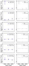 |
Fig. A.1. Comparison of the satellite velocity dispersion obtained using three different halo masses in the estimates of rvir and vvir. The left column shows the results for star-forming samples and the right column for the total samples. Different rows represent different stellar mass bins. In each panel, the three data points are for halo masses that correspond to 16, 50, and 84 percentage points of the mass distribution, respectively, as labeled on the horizontal axis. |
Appendix B: The Mh-σs relations for different stellar mass bins
To avoid the correlation between the uncertainties in σs and in the Mh-σs relation, we derived the Mh-σs relation using a slightly different method. For a given galaxy sample in a stellar mass bin, we used the complementary sample consisting of all galaxies in other stellar mass bins to fit the Mh-σs relation. The relations so obtained for different stellar mass bins are shown in Table B.1. As one can see, these relations are consistent with one another and with Eq. 4 within error bars. It is clear that the σs of a galaxy sample in a stellar mass bin is quite independent of the complementary sample used for the calibration. Thus, we can use the value of the σs for the galaxy sample, in combination with the corresponding Mh-σs relation, to derive the halo mass and conversion efficiency for the sample. The results are shown in Table 1.
Halo mass-satellite velocity dispersion relations.
Appendix C: Measurements with the SDSS shear catalog
As an independent test, we also used a different shear catalog (Luo et al. 2017) based on SDSS DR7 (Abazajian et al. 2009). The difference between the two samples is twofold. First, the shape measurement method here uses a traditional second-moment estimator to evaluate the ellipticity; secondly, the coverage of the SDSS DR7 is much larger than the DECaLS region that overlaps with our lens samples. There are 190,730 galaxies with M* ≥ 108.8 M⊙ in the star-forming sample and 445,135 galaxies with M* ≥ 108.8 M⊙ in the total sample. However, the deeper imaging, together with the PDF-symmetrization method, gives much smaller statistical errors than the SDSS DR7 catalog. We repeated the modeling as described above to extract the halo mass. The results are consistent with those obtained from the DECaLS shear data but with larger error bars, as shown in Fig. 5. The ESDs and best fitting results obtained from the SDSS shear catalog are presented in Fig. C.1.
Appendix D: The IllustrisTNG simulation used for comparison
The IllustrisTNG simulations were run with AREPO (Springel 2010), which implements a moving-mesh technique. The simulations include sub-grid physical models for gas cooling, star formation, metal enrichment, and stellar and AGN feedback. In this paper, we use the simulation TNG100-1, which has a box size of ∼100 Mpc. The dark matter particle mass is 7.5 × 10⁶ M⊙ and the average gas cell mass is about 1.39 × 10⁶ M⊙. Galaxies with M* ≥ 108.8 M⊙ are well resolved in the simulation. Central galaxies are defined as the most massive galaxies in their host halos. Galaxy stellar mass is the sum of all stellar particles within the gravitationally bound substructure, and the SFR is calculated from all gas cells in the same region. The halo mass, directly taken from the simulation, is the mass contained in spherical regions, within each of which the mean mass density is 200 times of the cosmic mean matter density.
In Fig. D.1 we show the SFR-stellar mass relation for central galaxies in the simulation. The simulation can reproduce the star-forming main sequence well, and most star-forming galaxies in the plotted stellar mass range are well above the demarcation line used in our observational data. We thus decided to use the same demarcation criteria to identify star-forming galaxies. The efficiency as a function of stellar mass for both star-forming galaxies and total galaxy populations is presented in Fig. 5.
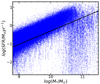 |
Fig. D.1. SFR−M* diagram for model galaxies. The figure shows the result for central galaxies in IllustrisTNG. The solid line is the demarcation line used to identify star-forming galaxies, which is the same as the one used in the observation. We note that a large fraction of the galaxies have very low SFRs. These galaxies fall outside the boundary of the plot. |
All Tables
All Figures
|
Fig. 1. Excess surface density (ESD) from the DECaLS shear catalog and the corresponding best fitting results. The symbols in the 12 panels show the ESD profiles obtained by stacking the lensing signals for galaxies in each stellar mass bin, as indicated in each panel. Results are shown separately for star-forming galaxies (first and third columns) and the total population (second and fourth columns). The error bars correspond to the standard deviation of 150 bootstrap samples. We fit the ESD by using three components, the stellar mass term (dotted lines with stars), the one-halo term (dashed lines), and the two-halo term (dash-dotted lines). The sum of these components are shown with solid lines. |
| In the text | |
|
Fig. 2. Distribution of the line-of-sight velocity difference (Δv) between central galaxies and their satellite candidates. The solid lines with error bars show the PDF of Δv. The dashed lines show the Gaussian-plus-a-constant fits to the data points. The error bars correspond to the standard deviation of 100 bootstrap samples. The upper row shows the results for star-forming centrals, while the lower row is for the total central population. The results of the star-forming and total samples in different stellar mass bins are shown in different columns. We note that the scales of the vertical axes are different for different panels. |
| In the text | |
|
Fig. 3. Halo mass–satellite velocity dispersion relation. The open (solid) diamonds show the velocity dispersion (σs) of satellites versus the host halo masses for total (star-forming) central galaxies. The halo masses are measured from DECaLS lensing data. Different colors indicate different stellar mass bins of central galaxies. The error bars for halo mass indicate the 16% and 84% of the posterior distribution obtained from the MCMC fitting to the stacked lensing profiles. The error bars for σs represent the 16% and 84% of the posterior distribution obtained from the fitting to the distribution of the satellite-central velocity difference. The solid line represents the best fit to the data points for the total galaxy sample. |
| In the text | |
|
Fig. 4. Stellar mass–halo mass relation. The red symbols with error bars show the SHMR calculated using the halo mass obtained from the fits to the stacked lensing mass profiles from the DECaLS shear catalog, while the black ones are based on the LcSK method. For clarity, we shift the black symbols slightly toward the left. The error bars reflect the 16% and 84% of the posterior distribution. The diamonds and squares show the results for star-forming and total populations, respectively. The shadow region represents the range covered by curves published in Yang et al. (2009), Moster et al. (2010), Leauthaud et al. (2012), Kravtsov et al. (2018), and Behroozi et al. (2019). |
| In the text | |
|
Fig. 5. Baryon conversion efficiency as a function of stellar mass. In the left panel, the symbols with error bars show the efficiency calculated using the halo mass obtained from the fits to the stacked lensing mass profiles. The black symbols show the results from the DECaLS shear catalog, while the green ones are obtained from the SDSS shear catalog (see Appendix C). The solid and open symbols show the results for the star-forming and total populations, respectively. Error bars indicate the 16% and 84% of the posterior distribution obtained from the MCMC fitting. In the right panel, the symbols with error bars show the efficiency calculated using the LcSK method. The error bars reflect the 16% and 84% of the posterior distribution obtained from the LcSK. The solid (dashed) gray lines show the results for star-forming (total) galaxies in the hydro-simulation IllustrisTNG. The shadow region in the two panels covers the range obtained before, as in Fig. 4. |
| In the text | |
|
Fig. 6. Ratio of the 2PCCF between star-forming galaxies and the total control galaxies as a function of the projected distance (rp) in different stellar mass bins. Error bars are the standard deviation of the 2PCCF ratio among 100 bootstrap samples. The horizontal dashed line in each panel indicates the theoretical ratio from a halo bias model (Tinker et al. 2010) that uses the halo mass measured from weak lensing as the input. For clarity, we only show the results for the four highest-mass bins, where the uncertainties in lensing mass measurements are relatively small. |
| In the text | |
|
Fig. 7. Comparison of our SHMR with those of Mandelbaum et al. (2016) and Bilicki et al. (2021). The diamonds, the lines with error bars, and the shaded regions are the SHMRs from our results, Mandelbaum et al. (2016), and Bilicki et al. (2021), respectively. The solid symbols show the results calculated using the DECaLS shear catalog. The red and blue represent the red and blue galaxy samples, respectively. |
| In the text | |
|
Fig. 8. Comparison of the MPA-JHU stellar mass with the stellar masses from NYU-VAGC (blue) and Salim et al. (2016) (red) for central star-forming galaxies. The solid lines show the median value of the residual, while the shaded regions show the 25% and 75% of the residual distribution. |
| In the text | |
|
Fig. 9. Probability distributions of galaxy concentration (C = R90/R50) for the total galaxy sample (green line) and the massive star-forming galaxy sample (black line) of M* ∼ 1011 M⊙. |
| In the text | |
|
Fig. 10. Rotation curves for two disk galaxies with a stellar mass of 1011 M⊙ but with a halo mass of 1012 M⊙ (star-forming, blue) and 1012.6 M⊙ (total, green). The two disk galaxies have the same stellar mass exponential profiles, with a disk scale length of 4.4 kpc and a Sèrsic index of n = 1. Dark matter halos are assumed to have an NFW profile with the concentration-mass relation from Zhao et al. (2009); c = 13 for the blue line, and c = 11 for the green line. |
| In the text | |
|
Fig. A.1. Comparison of the satellite velocity dispersion obtained using three different halo masses in the estimates of rvir and vvir. The left column shows the results for star-forming samples and the right column for the total samples. Different rows represent different stellar mass bins. In each panel, the three data points are for halo masses that correspond to 16, 50, and 84 percentage points of the mass distribution, respectively, as labeled on the horizontal axis. |
| In the text | |
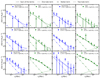 |
Fig. C.1. Same as in Fig. 1 but for the SDSS shear catalog. |
| In the text | |
|
Fig. D.1. SFR−M* diagram for model galaxies. The figure shows the result for central galaxies in IllustrisTNG. The solid line is the demarcation line used to identify star-forming galaxies, which is the same as the one used in the observation. We note that a large fraction of the galaxies have very low SFRs. These galaxies fall outside the boundary of the plot. |
| In the text | |
Current usage metrics show cumulative count of Article Views (full-text article views including HTML views, PDF and ePub downloads, according to the available data) and Abstracts Views on Vision4Press platform.
Data correspond to usage on the plateform after 2015. The current usage metrics is available 48-96 hours after online publication and is updated daily on week days.
Initial download of the metrics may take a while.