| Issue |
A&A
Volume 663, July 2022
|
|
|---|---|---|
| Article Number | A66 | |
| Number of page(s) | 28 | |
| Section | Extragalactic astronomy | |
| DOI | https://doi.org/10.1051/0004-6361/202142740 | |
| Published online | 14 July 2022 | |
Predicting Lyman-continuum emission of galaxies using their physical and Lyman-alpha emission properties
1
Observatoire de Genève, Université de Genève, Chemin Pegasi 51, 1290 Versoix, Switzerland
e-mail: This email address is being protected from spambots. You need JavaScript enabled to view it.
2
Univ. Lyon, Univ. Lyon 1, ENS de Lyon, CNRS, Centre de Recherche Astrophysique de Lyon, Saint-Genis-Laval, France
3
Research Center for Statistics, Université de Genève, 24 rue du Général-Dufour, 1211 Genève 4, Switzerland
4
Yonsei University, 625 Science Hall, 50 Yonsei-ro, Seodaemun-gu, Seoul 03722, South Korea
5
University of Oxford, Clarendon Laboratory, Parks Road, Oxford, UK
6
University of Cambridge, Madingley Road, Cambridge, UK
Received:
24
November
2021
Accepted:
1
April
2022
Abstract
Aims. The primary difficulty in understanding the sources and processes that powered cosmic reionization is that it is not possible to directly probe the ionizing Lyman-continuum (LyC) radiation at that epoch as those photons have been absorbed by the intervening neutral hydrogen. It is therefore imperative to build a model to accurately predict LyC emission using other properties of galaxies in the reionization era.
Methods. In recent years, studies have shown that the LyC emission from galaxies may be correlated to their Lyman-alpha (Lyα) emission. In this paper we study this correlation by analyzing thousands of simulated galaxies at high redshift in the SPHINX cosmological simulation. We post-process these galaxies with the Lyα radiative transfer code RASCAS and analyze the Lyα – LyC connection.
Results. We find that the Lyα and LyC luminosities are strongly correlated with each other, although with dispersion. There is a positive correlation between the escape fractions of Lyα and LyC radiations in the brightest Lyman-alpha emitters (LAEs; escaping Lyα luminosity LescLyα > 1041 erg s−1), similar to that reported by recent observational studies. However, when we also include fainter LAEs, the correlation disappears, which suggests that the observed relation may be driven by selection effects. We also find that the brighter LAEs are dominant contributors to reionization, with LescLyα > 1040 erg s−1 galaxies accounting for > 90% of the total amount of LyC radiation escaping into the intergalactic medium in the simulation. Finally, we build predictive models using multivariate linear regression, where we use the physical and Lyα properties of simulated reionization era galaxies to predict their LyC emission. We build a set of models using different sets of galaxy properties as input parameters and predict their intrinsic and escaping LyC luminosity with a high degree of accuracy (the adjusted R2 of these predictions in our fiducial model are 0.89 and 0.85, respectively, where R2 is a measure of how much of the response variance is explained by the model). We find that the most important galaxy properties for predicting the escaping LyC luminosity of a galaxy are its LescLyα, gas mass, gas metallicity, and star formation rate.
Conclusions. These results and the predictive models can be useful for predicting the LyC emission from galaxies using their physical and Lyα properties and can thus help us identify the sources of reionization.
Key words: radiative transfer / galaxies: high-redshift / ultraviolet: galaxies / galaxies: general / methods: data analysis / methods: statistical
© ESO 2022
1. Introduction
Cosmic reionization is an important period in the evolution of the Universe, when photons from energetic sources (i.e., first stars, galaxies, or quasars) ionized the ubiquitous neutral hydrogen gas in the intergalactic medium (IGM). This milestone happened over the first billion years of the Universe, ending at around z ∼ 6, and it holds a key for understanding the formation and evolution of the first galaxies (Loeb & Barkana 2001; Stark 2016; Ocvirk et al. 2016; Rosdahl et al. 2018; Wise 2019). However, the epoch of reionization (EoR) is yet to be fully understood. One of the biggest outstanding questions is determining the primary sources of the photons that ionize the Universe. The relative importance of the two types of sources proposed in the literature – star-forming galaxies and quasars – is still somewhat debated. However, recent studies indicate that quasars were likely too rare at these redshifts to reionize the Universe (Cowie et al. 2009; Fontanot et al. 2012, 2014; Kulkarni et al. 2019; Faucher-Giguère 2020; Trebitsch et al. 2021) and that photons from star formation are most probably the primary sources of reionization. Yet, it remains to be understood which types of galaxies are most profusely leaking ionizing radiation (photons with wavelength λ < 912 Å, also called the Lyman continuum) and the properties and environments that can make a galaxy a Lyman-continuum (LyC) leaker.
The primary difficulty in understanding the processes and sources that powered cosmic reionization is that it is not possible to directly probe the ionizing radiation at that epoch as those photons are all absorbed by the IGM on their way to us (Madau 1995; Inoue et al. 2014). Due to this, it is imperative to find indirect tracers for LyC emission to identify the sources of reionization.
In recent years, several methods have been proposed in the literature to indirectly measure LyC emission from galaxies: weak interstellar medium (ISM) absorption lines (Heckman et al. 2011; Erb 2015; Chisholm et al. 2017, but see Mauerhofer et al. 2021), a high [OIII]/[OII] ratio (Jaskot & Oey 2013; Nakajima & Ouchi 2014, but also see Bassett et al. 2019; Katz et al. 2020), and the Lyman-alpha (Lyα) line of hydrogen (Dijkstra 2014; Verhamme et al. 2015, 2017; Dijkstra et al. 2016; Izotov et al. 2018a). Among these, the Lyα line is particularly interesting. Since it is a UV line, Lyα is observable over a wide range of redshifts, allowing one to probe galaxy formation with the same tool over several gigayears of evolution. Indeed, over the last 20 years, a large number of Lyα-emitting galaxies have been observed: from the low-redshift Universe using space-based facilities, such as the Lyman Alpha Reference Sample (LARS) and the Extended LARS (eLARS) survey, which include 14 and 28 Lyman-alpha emitters (LAEs) respectively, at 0.03 < z < 0.18 (Hayes et al. 2013; Östlin et al. 2014) and the Green Pea sample of 43 LAEs at z = 0.2 (Henry et al. 2015; Schaerer et al. 2016; Yang et al. 2017); from the ground in the optical from z ∼ 2 to z ∼ 6 (several thousand spectroscopically confirmed LAEs; Erb et al. 2011; Bacon et al. 2015; Trainor et al. 2015; Urrutia et al. 2019); and in the IR at the highest redshifts; for example, the SILVERRUSH survey using the Hyper Suprime-Cam recently observed a large sample of 2230 LAEs at z = 5.7−6.6 with narrowband imaging data (Ouchi et al. 2018; Shibuya et al. 2018). At even higher redshift, it is increasingly difficult to detect LAEs due to the attenuation of Lyα by the relatively neutral IGM. However, concentrated efforts with very deep photometric and spectroscopic surveys in recent years have led to detections of some Lyα-emitting galaxies in the extreme redshift range of z = 6−9 (Vanzella et al. 2011; Ono et al. 2012; Schenker et al. 2012; Shibuya et al. 2012; Finkelstein et al. 2013; Oesch et al. 2015; Konno et al. 2014; Zitrin et al. 2015; Song et al. 2016; Roberts-Borsani et al. 2016; Stark et al. 2017; Matthee et al. 2017, 2018, 2020; Songaila et al. 2018; Itoh et al. 2018; Jung et al. 2019; Meyer et al. 2021). The upcoming James Webb Space Telescope (JWST) surveys are expected to discover many more such galaxies in the EoR soon.
The possibility of the relatively intense Lyα radiation from galaxies being a tracer of LyC emission has been studied a great deal in the past few years. Verhamme et al. (2015) explored the escape of Lyα and LyC in idealized galaxy models and found that Lyα line profiles show distinct signatures (a strong, narrow peak or a narrow peak separation if it is double-peaked) if the ISM of galaxies is transparent to the LyC. Dijkstra et al. (2016) found similar results in a theoretical study of a suite of 2500 idealized models of a dusty and clumpy ISM with Lyα radiative transfer simulations.
Verhamme et al. (2017) performed an observational study of LyC leakers in the sample of Green Pea galaxies (the local analogs of high-z LAEs) and found that in the eight galaxies where it is possible to detect LyC emission1 in addition to Lyα, the escape fractions of Lyα and LyC are indeed positively correlated. Recently, Izotov et al. (2021) observed nine more galaxies in both LyC and Lyα in the redshift range ∼0.30−0.45 and found that similar correlations exist in this sample as well. Steidel et al. (2018) studied the Keck Lyman Continuum Spectroscopic Survey sample, which includes 15 (out of 124) galaxies detected in LyC at z ∼ 3, and found that the LyC escape fraction is well correlated with the equivalent width of the Lyα emission.
The correlation between Lyα and LyC radiation shows great promise, but to use this in the reionization era to estimate the LyC from galaxies, we need to statistically analyze a large sample of EoR galaxies. Since LyC cannot be observed in this epoch, we need to explore it with simulations. Modeling Lyα and LyC radiation from a large sample of galaxies in simulations has been particularly challenging because it requires simulations to overcome several technical challenges. Such simulations need to incorporate LyC radiation transfer on the fly (i.e., coupled at each hydrodynamical time step) to describe the ionization state of each cell in the simulation volume accurately. These simulations also need to account for the radiative transfer of Lyα, which requires a fully parallel resonant scattering code. Finally, the production and scattering or absorption of Lyα and LyC photons happen at small scales in the ISM of galaxies, and their eventual escape or absorption is at galactic and intergalactic scales, so the simulation needs to sample both small and large scales correctly in order to predict reliable escape fractions and reionization topology. All of these requirements make such undertakings challenging and computationally expensive. Hence, simulation studies of this kind have so far generally focused on either analyzing a small volume with high resolution, such as isolated galaxies (Verhamme et al. 2012; Behrens & Braun 2014), Lyα nebulae or Lyα blobs (Yajima et al. 2013; Trebitsch et al. 2016), molecular clouds (Kimm et al. 2019), and zoomed-in simulations of individual galaxies (Faucher-Giguère et al. 2010; Smith et al. 2019; Laursen et al. 2019), or large volumes but with comparatively poor resolution (Yajima et al. 2014; Inoue et al. 2018; Gronke et al. 2021).
With this in mind, the SPHINX (Rosdahl et al. 2018) simulations are an ideal choice for this study, being a state-of-the-art radiation hydrodynamics (RHD) simulation, having a good balance of a sufficiently large volume and high resolution, and hosting a large sample of well-resolved galaxies. SPHINX is a suite of cosmological RHD simulations that reach a resolution of up to 10 pc in 10 co-moving Mpc (cMpc) wide volumes (Rosdahl et al. 2018). This allows us to investigate the Lyα and LyC properties of thousands of simulated galaxies at z > 6 (see Rosdahl et al. 2018; Garel et al. 2021).
In this paper we focus on the questions of whether there is a correlation between Lyα and LyC emission at galaxy scale during the EoR and whether it is possible to predict the LyC emission of galaxies if their physical and Lyα properties are known.
The paper is structured as follows. We discuss our methods in Sect. 2, where we describe the SPHINX simulation and the radiative transfer code that we use for Lyα post-processing and present our sample of simulated galaxies. In Sect. 3 we explore the relationship between LyC and Lyα luminosities and escape fractions and analyze the contribution of LAEs to reionization. In Sect. 4 we build a multivariate regression model where we use the physical and Lyα properties of galaxies to predict their intrinsic and escaping LyC luminosities and escape fractions, determine the most important variables required for each prediction, and apply our models to observed data for comparison. In Sect. 5 we discuss the limitations of our study, and in Sect. 6 we summarize our results.
2. Methods
In this section we present the simulation, the selection procedure to build our sample of galaxies, and our methods to calculate LyC and Lyα emissions from them.
2.1. Reionization simulation
SPHINX (Rosdahl et al. 2018) is a suite of cosmological hydrodynamical simulations of the EoR. In this study we analyze galaxies in the 10 cMpc wide SPHINX volume previously presented in Rosdahl et al. (2018), who used the binary stellar population model from BPASS (Binary Population and Spectral Synthesis code, Stanway et al. 2016).
SPHINX is run with the RAMSES-RT code (Teyssier 2002; Rosdahl et al. 2013). It simulates an average density patch of the Universe. The spatial resolution reaches 10.9 pc at z = 6, the dark matter mass resolution is 2.5 × 10⁵ M⊙ per particle and the stellar mass resolution is 103 M⊙ per stellar particle (we refer to Rosdahl et al. 2018, for details of the simulation). Within the simulation the radiation tracked is split into three photon groups, which encompass the ionization energies for HI, HeI, and HeII. These photons interact with hydrogen and helium in the simulation via photo-ionization, heating, and momentum transfer. The simulation is run until z = 6, and it uses Planck results (Planck Collaboration XVI 2014) for the cosmological parameters: ΩΛ = 0.68, Ωm = 0.32, Ωb = 0.05, h = 0.67, and σ8 = 0.83.
2.2. Halo and galaxy samples
We use the same halos and galaxies as described and analyzed in Rosdahl et al. (2018). In short, galaxies are detected in two stages. The group finder algorithm ADAPTAHOP (Aubert et al. 2004; Tweed et al. 2009) is run on the dark matter particles, and the over-dense virialized regions are identified as halos (and sub-halos, sub-sub-halos, etc., depending on their level of structure). Halos are considered to be resolved when they have virial masses (Mvir) greater than 300 times the dark matter particle mass (i.e., Mvir > 7.4 × 10⁷ M⊙). Then ADAPTAHOP is run on stellar particles, and it identifies the over-dense groups with at least ten stellar particles as galaxies. Finally, the most massive galaxy within 0.3 Rvir is assigned to each halo to build the galaxy-halo catalog.
In our analysis, we selected systems that have stellar mass M⋆ > 106 M⊙ (this is the stellar mass within 0.3Rvir of the halo) and where the main halo is at level 1 (i.e., they are not a substructure of a parent halo). We excluded less massive galaxies with M⋆ < 106 M⊙ from our sample and focus on bright galaxies that are potentially observable. This stellar mass limit also means that all of our galaxies contain at least 103 stellar particles, which ensures that the selected galaxies are reasonably well resolved.
We analyzed snapshots of the SPHINX simulation at five different redshifts: z = 6, 7, 8, 9, and 10. We selected all galaxies that satisfy our criterion described above. The numbers of selected galaxies at these redshifts are respectively 674, 509, 362, 236, and 152. Among the galaxies at 6 ≤ z ≤ 10, the maximum galaxy stellar mass is 1.33 × 10⁹ M⊙, and there are ten galaxies with M⋆ > 108 M⊙. We compared the properties of the galaxies at these different redshifts and found that there is no significant evolution in terms of physical or radiative (Lyα or LyC) properties (this is discussed further in Appendix A.1). Therefore, we combine our galaxy sample as a larger sample size can give better statistical significance for our understanding. Our final sample comprises 1933 galaxies.
Figure 1 shows distributions of their stellar mass, gas mass and star formation rate (SFR). We recall that the stellar mass distribution in this figure shows the stellar mass within 30% halo virial radius. The median stellar mass is 106.41 M⊙.
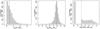 |
Fig. 1. Histograms of physical properties of the simulated galaxies in our sample. The histograms show the distribution of the stellar mass (left), gas mass (middle), and SFR10 (right) of the galaxies. The median values are shown by dashed black lines. The stellar mass histogram shows M⋆ within 30% of the halo virial radius. There are ten galaxies with M⋆ > 108 M⊙. The gas mass has a peaked distribution, with a few galaxies having very little gas (further discussion in Sect. 5). There are 943 galaxies with zero SFR10; these galaxies are represented in the bar at 10−6 (discussed in Sect. 4.2.1). |
The gas mass shown in Fig. 1 is the total gas mass of the halo, calculated by summing up the mass of all the gas cells inside Rvir. We find that the gas mass has a normal distribution (median mass 107.84 M⊙) with some halos containing very small amounts of gas, likely because a recent supernova or starburst has blown the gas away from these small systems.
The SFR10 shows the SFR of the galaxy averaged over the last 10 Myrs. This is a typical lifetime of massive stars, after which they undergo a supernova (the most massive stars live for about 3 Myr), and 10 Myr is also the typical timescale of the production of LyC and Lyα. In Fig. 1 we show the distribution of the log SFR10. There are 943 galaxies in our sample that have SFR10 = 0. We artificially set their SFR values equal to 10−6 M⊙ yr−1 (which is lower than the lowest nonzero SFR) to show them in the histogram. The median value of SFR10 is 10−4 M⊙ yr−1.
2.3. LyC emission from SPHINX galaxies
The production and escape of LyC photons in SPHINX has been described in Rosdahl et al. (2018). In short, the instantaneous escape fractions of LyC photons are calculated in post-processing, using RASCAS (Michel-Dansac et al. 2020). Rays are traced from every stellar particle inside a halo out to its virial radius. Along each ray, the optical depth (τ) is calculated for hydrogen and helium. For each stellar particle, the escape fraction is the average of e−τ calculated with rays in 500 random directions. Then the global escape fraction of the halo ( ) is the luminosity-weighted average escape fraction of all the stellar particles inside the halo. The LyC photons we consider range from 0−912 Å and in the simulation they are described in three groups of photons: photons that ionize HI (UVHI, 912–504 Å, 13.6–24.59 eV), HeI (UVHeI, 504–228 Å, 24.59–54.42 eV) and HeII (UVHeI, 228–0 Å, 54.42–∞ eV). The distributions of intrinsic (
 ) and escaping (
 ) LyC luminosities, and escape fractions for our galaxy sample are further described in Sect. 3.2.
On the contrary, observations of LyC usually focus on a small part of the ionizing spectrum, close to the Lyman limit (912 Å). This observed LyC luminosity, known as  (i.e., the escaping LyC luminosity at 900 Å), is defined as
 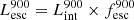 (
( and
and  are intrinsic luminosity and escape fraction at 900 Å, respectively). So we perform additional LyC measurements more similar to what is done observationally. We can estimate the intrinsic LyC luminosity of the simulated galaxies at 900 Å (
 ), using the BPASS models (Stanway et al. 2016) that have been used in modeling the ionizing emission in the SPHINX simulation. Using RASCAS, we distributed 105 photon packets with wavelengths between 10 and 912 Å among the stellar particles and then transferred them until they are absorbed by HI, HeI, HeII, or dust or escape the halo virial radius. Thereafter we have both the intrinsic and escaping spectral energy distribution from 10–912 Å, and this allows us to derive the LyC escaping luminosity and escape fraction over different wavelength ranges, for example 890–912 Å. The average luminosity in this range is the luminosity at 900 Å (i.e.,
  and
and  are in units of erg s−1/Å).
Figure 2 (left and middle panel) shows the ratio of total LyC (i.e., 0–912 Å) emission (intrinsic and escaping luminosities) to the LyC emission at 900 Å as a function of their total escaping LyC ( ) luminosities for all simulated galaxies. Since we integrate over a wavelength range 900 times larger for the total luminosity, we expect a rough ratio of around 900 between the two intrinsic luminosities. The ratio of the escaping luminosities is expected to be higher because the cross-section of hydrogen photoionization is approximately proportional to λ3 at λ < 912 Å, so
  could be more attenuated than
  . Indeed, the median ratios for intrinsic and escaping luminosities are 1036 and 1536, respectively. We also find that this ratio for both intrinsic and escaping luminosities has a significant scatter, probably due to the particular star formation history and morphology of each galaxy.
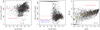 |
Fig. 2. Ratio of total intrinsic (left) and escaping (middle) LyC luminosity emitted over the range of 0–912 Å and the intrinsic and emitted LyC at 900 Å, as a function of their total escaping LyC luminosity. The median ratio calculated with all simulated galaxies is shown with the dashed red line. Some of the galaxies have |


In particular, we find that 242 galaxies (i.e., 12% of our galaxies) have  ; in other words, for these galaxies,
  , and these ratios are represented at a value of 4250 in the middle panel. Almost all of them are also faint in total LyC emission, with only six having
  ergs s−1. This result suggests that few LyC leakers will be missed by surveys that probe only the flux close to the Lyman limit.
By comparing the number of intrinsic photons with the escaping photons, we also obtain the escape fraction at 900 Å. We show the ratio of  to
to  as a function of
  in the right panel of Fig. 2 and find that, except for a very few galaxies (with low luminosities),
  is lower than
  . The overall median ratio is 0.69. Kimm et al. (2019) also finds similar ratio while investigating the escape of LyC radiation from turbulent clouds. We divide the (log)
  into groups of 0.5 dex each and find that the median ratio increases slightly with
  .
.
2.4. Lyα emission from SPHINX galaxies
In order to investigate the correlation between LyC leakage and the observable Lyα properties of galaxies, we now turn our interest to the Lya post-processing of SPHINX galaxies.
A Lyα photon (wavelength –1215.67 Å, energy –10.2 eV) is emitted when a hydrogen electron jumps from the 2 p to the 1 s (ground) state. It is not only the hydrogen line with the largest flux, but also a resonant line. To obtain the Lyα properties of galaxies in the SPHINX simulation, we post-process them using RASCAS (Michel-Dansac et al. 2020), which is a fully parallelized 3D radiative transfer code developed to perform the propagation of any resonant line in numerical simulations. It performs radiative transfer on an adaptive mesh using the Monte Carlo technique. We describe below the different steps of our implementation.
Lyα intrinsic luminosities: Lyα emission can be triggered by two processes, recombination and collisional de-excitation (Dijkstra 2014). LyC photons from massive stars in galaxies ionize the neutral gas in their ISM and afterward, the free proton and electron recombine. The electron can initially enter into any energy level, and then cascades to ground level with a probability of ≈0.67 to emit a Lyα photon (Partridge & Peebles 1967; Dijkstra 2014). Alternatively, HI atoms can be excited collisionally, and when the electron returns to the ground state, a Lyα photon can be emitted. So, for any given halo in our sample, we track both recombinations and collisional excitations from all cells inside the halo virial radius to capture the intrinsic Lyα emission. For recombinations, the Lyα photon emission rate in each cell is (Cantalupo et al. 2008)
 (1)
(1)
where ne and np are the number density of electrons and protons, respectively (these come from the simulation), αB(T) is the case-B recombination coefficient,  is the fraction of recombination events that produces a Lyα photon eventually (at T = 104 K, it is 0.67) and (Δx)3 is the cell volume. For collisional excitation, the Lyα emission rate is given by (Goerdt et al. 2010)
 (2)
(2)
where nHI is the number density of neutral hydrogen, and CLyα(T) is the rate of collisionally induced 1s-to-2p level transitions (we do not consider higher order transitions). We refer to Michel-Dansac et al. (2020) for a detailed description of how we fit each of the coefficients αB(T),  and CLyα(T). Once these luminosities are known in each cell, we emit a total of 105 photon packets from the cells inside a galactic halo with the probability of a cell emitting a photon packet proportional to its luminosity. The number of photon packets has been chosen so as to minimize the computational cost while preserving the accuracy of the Lyα angle-averaged escape fraction and luminosity. Performing convergence tests on the ten most massive galaxies in our sample, we find that these quantities are well converged using 105 photon packets.
Lyα propagation and escape: In each cell, we cast Lyα photons isotropically and propagated them through the halo with the RASCAS code. Each Lyα photon can be scattered (i.e., absorbed and reemitted) numerous times whenever they encounter HI atoms in the ISM, until they finally escape the halo or are absorbed by dust. The dust is modeled by specifying a cross section per hydrogen atom and a pseudo dust number density that is dependent on HI and HII density and metallicity (Michel-Dansac et al. 2020). The dust absorption coefficient in each cell is given by (nHI + fionnHII) σdust(λ)Z/Z0, where fion = 0.01 (abundance of dust in ionized gas), Z is the gas metallicity in that cell, and the effective dust cross section, σdust, and Z0 (= 0.005) are normalized to the Small Magellanic Cloud models following Laursen et al. (2009).
The boundary beyond which a Lyα photon can be considered as having escaped is not an obvious choice. At z ≥ 6 where reionization takes place, configuration of galaxies are complex, partly because in many cases galaxies are interacting or colliding with each other. So we perform convergence tests on the ten most massive galaxies in our sample. In each of them, we set the boundary at Rvir, 2Rvir, and 3Rvir where Rvir is the corresponding halo virial radius, and run Lyα radiative transfer in each case. We find that beyond Rvir, the escape fraction converges, with only small increments in accuracy. So we fix Rvir to be the boundary of Lyα escape. Both the production and the propagation of photons are allowed within this radius, which encompass the main galaxy and in many cases, its satellites.
We used the core-skipping method to speed up the calculation (Michel-Dansac et al. 2020). We tested the core-skipping method by simulating the Lyα radiation transfer in the ten most massive galaxies in our simulation with and without core-skipping and found that the Lyα results, for example luminosities and escape fraction, are very similar (median 0.6% difference) and we gain significant (up to a factor of 100) speedup in the calculation. The distributions of intrinsic and escaping Lyα luminosities, and escape fractions, for our galaxy sample, are further described in Sect. 3.2.
3. LyC–Lyα relationship
The goal of our study is to investigate the connection between the Lyα and LyC properties of galaxies in order to investigate if, or how, Lyα can trace the total ionizing radiation escaping from galaxies at EoR. To that end, in this section we first discuss the relationship between their intrinsic and escaping luminosities and then analyze their escape fractions.
3.1. Observed LyC emitters
Before we explore the relationship between the various Lyα and LyC properties, we review existing observed sample of LyC emitters (LCEs) in order to facilitate the comparison of our simulated galaxies with observed ones.
Although there are many observations of Lyα at different redshifts, it is difficult to observe LyC even at low-redshift galaxies because Earth’s atmosphere blocks UV radiation, so no ground based observations are possible. However, in recent years it has become possible to obtain direct observations of LyC leakers using space-based facilities, for example the Hubble Space Telescope (Verhamme et al. 2017; Izotov et al. 2016a,b, 2018a,b, 2021). We compile these observations (23 galaxies) in Table 1, where we note their redshift, available physical properties (i.e., stellar mass, SFR, surface SFR density, escaping luminosity, and escape fraction in LyC and Lyα). The SFR is derived from Hβ observations and therefore correspond to SFR on a short timescale. They can thus be considered similar to the SFR10 in our simulated galaxies.
Observed data.
Figure 3 shows a comparison of the physical properties of these observed LCEs with our simulated sample. We find that the Lyα luminosities of the SPHINX galaxies do not scale well with stellar masses, gas metallicities, or galaxy sizes, whereas they do correlate with recent star formation, as expected since a higher SFR means that more energetic photons, which can be reprocessed in the ISM as Lyα, are being produced. The SFR10 of the galaxies correlates weakly with the stellar mass and has a large scatter. Because of the finite volume of our simulation, our sample is restricted to relatively faint and low-mass galaxies such that most of the observed objects considered here are brighter, slightly more massive, slightly bigger and have higher star formation than our simulated sources. The observed galaxies also have higher metallicities compared to the simulated ones, which is perhaps not surprising as the observed sample is at a much lower redshift (z ∼ 0.3 compared to z ∼ 6), and hence they can be more metal enriched. While this certainly represents a limitation of our study, investigating the LyC-Lyα connection in our sample can still be used to interpret available observational data and guide future surveys that will target galaxies more similar to our sample.
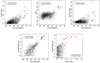 |
Fig. 3. Comparison of physical properties of observed LCEs (magenta points) and the simulated galaxies (black points). Here we show the stellar mass (top left), gas metallicity (oxygen abundances, i.e., 12 + log10(O/H) for observed galaxies, top middle), galaxy radius (galaxy virial radius for simulated ones and exponential disk scale length for observed ones, top right) and SFR (SFR10) as a function of their escaping Lyα luminosities. The Lyα luminosities of the SPHINX galaxies do not scale with stellar masses, metallicities, or galaxy sizes, whereas they do correlate with recent star formation, as expected. Top-right panel: we show the SFR (SFR10 for simulated galaxies) as a function of the stellar mass of galaxies. The properties of the observed LCEs are listed in Table 1, and more details can be found in their corresponding reference papers. |
It is important to note that the LyC luminosity in the Table 1 is  (i.e., the LyC luminosity at 900 Å). However, the escaping LyC luminosity that counts for reionization is the total luminosity of all photons that can ionize HI (i.e., all photons with λ = 0−912 Å), so we consider this total LyC throughout the paper. These two measures of LyC luminosities can be very different as discussed in Sect. 2.3, and the contribution of the highly ionizing spectrum for observed LCEs (< 900 Å) is still largely unknown. Since the observed LCEs are brighter in Lyα (> 1041 erg s−1) than the bulk of our galaxies, we recalculate the median of the
  /
/ ratio for bright LAEs and find the ratio to be 1434 (Fig. 2, middle panel). This ratio can be used to convert observed 900 Å luminosities to total LyC luminosities, if needed.
As we are interested in investigating the global theoretical connection between Lyα and the ionizing radiation of galaxies in the EoR, hereafter we consider the global Lyα and LyC photon budgets from galaxies, that is, summed over all directions and relevant wavelengths (i.e., 0–912 Å for LyC luminosities and  ) unless otherwise specified.
3.2. Distributions of Lyα and LyC properties
Figure 4 shows the distribution of the Lyα and LyC properties of our simulated galaxy sample, namely their intrinsic luminosities, escaping luminosities and their escape fractions. In all four cases (intrinsic and escaping for Lyα and LyC), the luminosities have a peaked distribution. The median values of  and
and  are 39.88 and 39.51 erg s−1 (in log scale), respectively, with the maximum escaping luminosity at 1.375 × 1042 erg s−1. The LyC luminosities show a similarly peaked distribution with median (log) values at 40.23 (
 ) and 38.80 (
 ). We note that the maximum luminosities of simulated galaxies are a consequence of the finite volume of the simulation box and the low end of the luminosities are affected by galaxy mass selection and the mass resolution of the simulation (Garel et al. 2021).
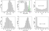 |
Fig. 4. Histograms of Lyα and LyC emission of our sample of 1933 galaxies. Top row: Lyα properties of our sample with intrinsic luminosity (left), escaping luminosity (middle), and escape fraction (right). Bottom row: same properties but for LyC radiation. In the middle panel of the top row, we also show the distribution of |


In contrast,  shows a bi-modal distribution with the major peak at 1 (the minor peak is at 0). We find that 32% of the sample has
  . The distribution of
  shows that most galaxies have low
  , with 62% of galaxies with
  . Since LyC can be absorbed by HI and HI is plentiful in the ISM, it is very hard for LyC to escape, resulting in very low
  in most galaxies. Lyα on the other hand is absorbed only by dust, so has a easier time to escape, which results in the peak around
  .
.
Among these six quantities, only the escaping Lyα luminosity is observable at the EoR. Our sample is fainter than most available LAE data but it can still be compared with the faint LAEs from MUSE (Multi Unit Spectroscopic Explorer) surveys. Therefore, in the histogram of  in Fig. 4 we also show the distribution of
  from galaxies in MUSE surveys. The MUSE data are taken from the MUSE-Deep survey (Drake et al. 2017) and MUSE Extremely Deep Field (Bacon et al., in prep.). In total, there are 892 MUSE galaxies in the redshift range of z = 2.92−6.64 with luminosities 1040.33−43 erg s−1. Among these, 21 galaxies are at z > 6. We see that there is overlap between the most luminous end of our simulated galaxies and the faint end from MUSE, in the luminosity range of ∼1040−42 erg s−1. Our simulated luminosities are the total Lyα output of the galaxy in all directions, before IGM attenuation. The observed data are, of course, directional measurements after IGM attenuation. We discuss the potential observational biases toward bright galaxies, and the lack of very bright LAEs in our sample due to the simulation box size limit in Sect. 5.
3.3. Investigating the Lyα-LyC luminosity relationship
To assess possible correlations between the LyC and Lyα radiation in galaxies, as a first step we analyzed their intrinsic and escaping luminosities.
In Fig. 5 we show the LyC luminosities of galaxies as a function of their Lyα luminosities. We find that for intrinsic luminosities, Lyα and LyC have a fairly tight positive correlation. The production of both LyC and Lyα is strongly related to the SFR of the galaxy because massive stars directly emit LyC photons and these same photons generate Lyα by photo-ionizing the HI in the ISM, which then can produce Lyα through recombination.
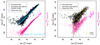 |
Fig. 5. LyC luminosity of galaxies as a function of their Lyα counterparts. Left: intrinsic LyC luminosity of galaxies as a function of their intrinsic Lyα luminosity. The black and pink points show the total LyC luminosity (0–912 Å) and the 900 Å luminosity of the simulated galaxies, respectively (Sect. 3.1). The diamond-shaped magenta points show the observed LCEs described in Table 1. The sky blue points show the intrinsic luminosities derived from the analytic model described in this panel. Right: escaping LyC luminosity of galaxies as a function of their escaping Lyα luminosity. The solid yellow line shows the median |


Furthermore, we also show their intrinsic LyC luminosity at 900 Å (as discussed in Sect. 2.3), and find that the intrinsic luminosities of observed LCEs (derived as observed luminosity/escape fraction) also fall on the same tight correlation, though extending to higher luminosities. This suggests that the correlation between intrinsic Lyα and LyC luminosities is valid over a large range of Lyα luminosities.
In the same figure we also show predictions for intrinsic Lyα luminosities from a simple model based on case B recombination (Spitzer 1978) given by, 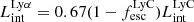 . This model assumes that all LyC photons that do not escape the galaxy will ionize the neutral hydrogen gas in the ISM. It also assumes that 67% of them will be reprocessed as Lyα photons through recombinations.
We find that the simulated data are generally matched well by this model. Some galaxies, especially among lower Lyα luminosity galaxies, lie below the analytical relationship, implying that the contribution of collisions is increasingly important for faint and low-mass Lyα emitters. For example, we find that in galaxies where  erg s−1, collisional emission contributes only a few percent of the total Lyα production, but it can rise to ∼50% in galaxies
  erg s−1 (see discussion and figure in A.2, also Rosdahl & Blaizot 2012). We also find that in all luminosity ranges, some galaxies fall above the analytical relationship, that is, there are some galaxies that have less Lyα production than estimated by the analytical equation. This is mainly due to the fact that a fraction of the most energetic photons go toward ionizing He or HeI, rather than HI, and as a result they cannot be reprocessed as Lyα. We also note that galaxies at the very faint end of Lyα (
 erg s−1) have LyC luminosity in the range of 1038 − 1040 erg s−1. These galaxies are extremely gas deficient, so they produce very little Lyα and the stars in them continue to produce LyC for a long time (further discussed in Sect. 5).
Furthermore, from the right panel of Fig. 5 we find that the escaping luminosity of Lyα and LyC is also well correlated. The escaping Lyα and LyC luminosities of the observed LCEs are also shown in this figure along with the  of the simulated galaxies and these LCEs seem to follow the similar trend. We note that the correlation is tight at higher luminosities, although the scatter is overall larger compared to the correlation between the intrinsic luminosities. The scatter increases as the galaxies become fainter in Lyα (or LyC). This is mostly due to the fact that the faint LAEs have a very wide range of Lyα and LyC escape fractions (discussed further in Sect. 3.5, see also Figs. 7 and 8). Hence, galaxies with similar intrinsic luminosities can end up with very different escaping luminosities, which scatters the points horizontally and vertically. The escape fractions of the galaxies depend on the structure of the ISM, in particular on the possibility of having holes or low HI column density channels in the ISM, which can facilitate the escape of LyC. We discuss the escape fractions in more detail in the next section. We also show this figure color-coded with
  and
and  in Fig. A.3 and further discuss the relationship of escaping luminosities with escape fractions in Appendix A.3. Moreover, we note that there are no galaxies with simultaneously very low Lyα and LyC luminosities. This is an effect of the stellar mass limit we imposed on our galaxies. We recall from Sect. 2.2 that we analyze here all galaxies with M⋆ > 106 M⊙. We checked that if we do include less massive galaxies in our sample, they start to fill up this faint section of the plot, as they are very faint in both Lyα and LyC. The few extremely faint LAEs we do have in our sample are extremely gas deficient, as we discussed in the previous paragraph, so it is easy for the LyC emission to escape from these systems; hence, their intrinsic and the escaping LyC luminosities remain almost same.
3.4. Fraction of LyC leakers in LAE samples
As shown in the previous sections, Lyα and LyC luminosities are correlated with one another. Hence, we can wonder what fraction of LAEs would be detectable as LyC leakers, assuming typical LyC and Lyα detection limits. To answer this question, we divide galaxies in our sample with  between 1038 and 1042.5 erg s−1 into nine equally logarithmically spaced bins (bin width 0.5 dex). In each group we calculate the median Lyα luminosity and the fraction of galaxies that have their
  luminosity higher than a given threshold value and report these fractions against their median
  in Fig. 6. We do this exercise for three different threshold values of escaping LyC luminosity, LThreshold = 1037, 1038, and 1039 erg s−1 and we find that as galaxies become brighter in Lyα, the fraction of galaxies with
  increases. For example, given a threshold LyC luminosity of 1038 erg s−1, 65% of LAEs with luminosity
  erg s−1 and 97% of LAEs with luminosity
  erg s−1 are bright in LyC emission. Granted, our simulated galaxies are at high redshift (z = 6−10) but these results could be useful at lower redshifts, where LyC emission can be detected. Katz et al. (2019, 2020) have shown that low metallicity LyC leakers at z ∼ 3 are good analogs of EoR galaxies. The observed
  limit around z = 3 is ∼1.61 × 1039 erg s−1 (flux limit 2 × 10⁻²⁰ erg s−1/cm2/ Å or 5.5 × 10⁻⁴ μJy; Kerutt et al., in prep.). At this threshold LyC luminosity, our analysis highlights that among LAEs with luminosity 1041.5−42 erg s−1, ∼15% of galaxies will be detected as LCEs.
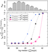 |
Fig. 6. Fraction of galaxies with |

3.5. Escape fraction
Figure 7 shows the  relationship of our simulated galaxies. Here we have plotted galaxies with progressively brighter sample selections: all galaxies (N = 1933), galaxies with
  erg s−1 (N = 1396), > 1040 erg s−1 (N = 598), and finally > 1041 erg s−1 (N = 150). We find that if we consider all 1933 galaxies, including the very faint ones, the escape fractions of Lyα–LyC are very scattered and not correlated. The escape fractions occupy the whole space above the equality line, with only a few galaxies with
  . However, if we limit our sample to only Lyα bright galaxies, the dispersion decreases. If we include only the brightest galaxies with
  erg s−1, a positive correlation emerges between the two escape fractions. A linear regression of these bright galaxies yields the following model (with standard errors),
  . We find that the observed LCEs (Table 1), which are all bright LAEs (> 1041 erg s−1), fall in the same escape fraction range as the simulated galaxies; this is an encouraging indication that the escape fractions of our simulated galaxies are not significantly different from the escape fractions calculated from observed local LCEs. The correlation between
  and
and  in the simulated bright galaxies and the observed ones is also very similar. This analysis indicates that the linear positive correlation of
  and
and  that we find in observed LCEs (Verhamme et al. 2017) may be a selection bias that holds true only when we consider the brightest LAEs.
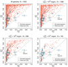 |
Fig. 7. Escape fractions of Lyα vs. LyC. The plots here show progressively brighter sample selection for all galaxies (top left) and galaxies with |


Additionally, in Fig. 7 we find that in galaxies with very low  , the
, the  can take any value between 0 and 1, but in galaxies with high
  , the
, the  is always very high. Conversely, galaxies with low
  always have low
  , but in galaxies with high
  ,
,  can range from 0 to 1. Dijkstra et al. (2016) also found similar distributions using idealized models. We also note that
  is always greater than
  , except for a few outlier galaxies in our simulated sample where
  . Theoretically it is expected that the Lyα escape fraction is greater than LyC because Lyα is only destroyed by dust while LyC can also be killed by HI atoms in the ISM. Lyα photons can scatter numerous times and have a greater possibility to find channels in the ISM with low HI column density through which they can escape the galaxy (Dijkstra et al. 2016). However, in 6 out of 1933 (or 0.3%) of our galaxies we find that this is not the case. Similarly for observed LCEs, although most of them have higher
  , in 2 out of 23 galaxies ( 8.7%),
  is less than
  . It is possible that in these systems there are dusty escape channels with low HI column density (the dust model allows for dust in ionized gas) such that it is optically thin to LyC photons but not to Lyα. We looked into these six simulated galaxies and found that these systems comprise interacting galaxies with complex configurations. The distributions of Lyα and LyC sources differ, and they have escape channels of low density gas columns very close to the center, where LyC production happens, which can greatly aid LyC escape.
3.6. Median escape fraction at different Lyα luminosities
Since we have a large sample of galaxies with both Lyα and LyC radiative transfer, it is instructive to study how  and
and  correlate with the Lyα luminosity of galaxies. To analyze this, we took all galaxies in our sample with
  from 1038 to 1042.5 erg s−1 and divided the luminosities into nine equally logarithmically spaced bins (bin width 0.5 dex). We show the median escape fractions against median luminosities in Fig. 8 and find that as the luminosity increases
  decreases. The drop in
  is fairly gradual and in our highest luminosity bins, 1041.5−42.5 erg s−1, the median value of
  is ∼0.3. Brighter galaxies have higher mass in all components, including dust mass, and as dust content increases, more Lyα is absorbed by dust, which reduces
  . At the bright end,
  erg s−1, our sample size decreases to only a couple of galaxies, owing to the limited simulation volume. Therefore, although the flattening of the median curves in bright LAEs suggests a similar value for even brighter galaxies, we cannot make any concrete prediction for much brighter LAEs.
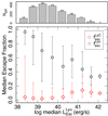 |
Fig. 8. Median |


The median  is low for all Lyα luminosities. In galaxies with
  erg s−1 median
  is very low (∼0.02), and in brighter galaxies it rises to ∼0.1. A large fraction of faint LAEs have zero or very low
  since ionizing photons are absorbed by HI gas in the surrounding ISM, which drives the median low (Chuniaud et al., in prep.).
The median Lyα luminosity of MUSE LAEs is around 1041.6 erg s−1, as shown in Fig. 4. Our simulation predicts that the typical  and
and  of galaxies at this luminosity are around 0.3 and 0.1, respectively. Here we note that the Lyα luminosities of MUSE galaxies are what we observe after Lyα has gone through IGM attenuation. The escaping Lyα luminosity of galaxies can be affected adversely by IGM attenuation, especially at z > 6. In our simulation we did not consider the effects of IGM. Along the same lines, the observed luminosities of MUSE galaxies are what we measure along our line of sight, whereas the simulated luminosities and escape fractions quoted here are global ones. We provide further discussion on the effects of IGM attenuation and line-of-sight variability in Sect. 5.
3.7. Contribution of LAEs to reionization
In our analysis, we have both ionizing or LyC luminosities and the Lyα luminosities for a large sample of simulated galaxies in EoR, so we can investigate the role of LAEs as sources of cosmic reionization. Similar to the previous section, we take our sample of galaxies that have Lyα luminosities in the range 1038 − 1042.5 erg s−1 range and divide them into nine equally logarithmically spaced bins (bin width 0.5 dex). For each group of galaxies we calculate their total escaping ionizing luminosities and plot it as a function of their median escaping Lyα luminosity in Fig. 9 (left panel). We find that as galaxies become brighter, their total escaping LyC luminosity in each group increases. Since our 10 Mpc3 simulation volume does not contain galaxies brighter than 1.35 × 1042 erg s−1 (see also the Lyα luminosity functions, e.g., Fig 5, in Garel et al. 2021), there is a downward trend at the extreme bright end of our sample (1041.5−42). Therefore, our sample size is too small to be conclusive about a peak at 1041 erg s−1. Nevertheless, the luminosity range of 1038 − 1041 erg s−1 is well sampled, and we find that in this luminosity range, the brighter LAEs have higher total  .
.
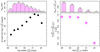 |
Fig. 9. Total escaping ionizing luminosity of LAEs. Left: total escaping LyC luminosity of galaxies grouped by their Lyα luminosities as a function of their median Lyα luminosity. The histogram above shows the number of galaxies in the corresponding bins below. Right: conditional total escaping LyC luminosity of galaxies brighter than a given Lyα luminosity limit as a function of the Lyα luminosity limit. The histogram above indicates the number of galaxies where |

Now we calculate the total ionizing luminosity in the whole simulation box. We recall that our galaxy sample consists of galaxies with the selection criteria provided in Sect. 2.2 (i.e., galaxies at level 1 and with M⋆ > 106 M⊙). Then, to be consistent in our comparisons, we estimated the total ionizing luminosity in the box by summing up the LyC luminosity ( ) of all galaxies at level 1 (i.e., from a total of 8783 such galaxies in our simulation).
We compute the contribution of galaxies with Lyα luminosity brighter than some limit to the total ionizing luminosity emitted by all simulated galaxies. The result of this is shown in the right panel of Fig. 9. We find that simulated LAEs brighter than 1040 erg s−1 (N = 598) contribute more than 90% to the total ionizing luminosity of the box, even though the number of faint LAEs is much larger than bright ones. So 6.8% (598 out of 8783 galaxies) of the galaxies, which hosts 37% of total stellar mass, are responsible for more than 90% of the escaping ionizing radiation. Including all LAEs brighter than 1038 erg s−1 (N = 1856) can account for ≈95% of the total LyC luminosity.
In the MUSE Ultra Deep Field survey (Fig. 5; Drake et al. 2017) at z = 3 the Lyα luminosity limit is 1041.25 erg s−1 (50% completeness). Our analysis suggests that the LAEs with  erg s−1 at EoR could have contributed ∼57% of the ionizing radiation budget.
The faint LAEs produce a small amount of LyC intrinsically, compared to the bright LAEs (Sect. 3.3). From our analysis of escape fractions in the previous section we know that the median  of all galaxies is rather low. Consequently the escaping LyC luminosities of faint LAEs is generally low. Therefore, we find that although faint LAEs are far more numerous, brighter LAEs as a group contribute more to the escaping ionizing luminosity. We also explored the effect of the lower mass limit of the galaxies (discussed further in Appendix A.4) on this reionization study and found that if we lower the mass limit of our galaxies from 106 to 105 M⊙, LAEs brighter than 1040 contribute 97% of the total ionizing radiation (Fig. A.4). This shows that although lowering the mass limit slightly increase these fractions, the differences are very small, our results thus converge. Therefore, we conclude that the primary sources of reionization are likely bright LAEs with
  erg s−1.
4. Predicting LyC luminosities and escape fractions
The major goal toward studying the connection between Lyα and LyC emission from galaxies is to discover a correlation or develop a model that can estimate the LyC emission of EoR galaxies using the observable properties of galaxies, as the ionizing photons themselves cannot be observed.
In the previous section (Sect. 3) we found that the escape fractions of Lyα and LyC are correlated in bright LAEs during the EoR, as observations have suggested, but when we include all LAEs in our sample, including the fainter ones, there is no correlation, which implies that the observed relation may be due to a selection bias. We also found that the intrinsic luminosities in Lyα and LyC are well correlated, whereas the escaping luminosities have a positive correlation but with much more dispersion, especially at the faint end. Thus, in the quest for predicting the LyC emission, it is important to explore beyond the simple 1:1 correlation. Since we have a large data set of galaxies with a number of their physical, Lyα and LyC properties we now investigate if it is possible to construct a statistical model that predicts the LyC emission using other properties (e.g., mass, SFR, and Lyα).
Our galaxy sample is generally fainter (highest  erg s−1) and less massive (highest stellar mass M⋆ ∼ 1.33 × 10⁹ M⊙) than typical observed LAEs. The model that we can build with these data can be best applied to galaxies with properties similar to SPHINX galaxies. Whether this model can be applied to more massive or more luminous galaxies cannot be conclusively determined based on this study alone. Nevertheless, building such a predictive model for LyC using our data is an important first step toward a quantitative understanding of the contribution of galaxies to reionization. This analysis will also identify which galaxy properties are the main predictors of LyC emission and this can help identify strong LCEs among observed samples of EoR galaxies and guide future surveys.
4.1. Multivariate model: A general framework
In our simulation we have a large data set of hundreds of galaxies each with several physical and radiative properties that can be measured in their real-world counterparts. Given the large number of variables available, we aim to build a model that can be interpreted easily. Multivariate linear regression is a common statistical method for building such models, it is also straightforward to interpret and gain insights from the final model.
Recently, Runnholm et al. (2020) did an analysis where they applied multivariate linear regression to observed galaxies at low redshift to predict escaping Lyα luminosities using observed galaxy properties. In this study, they have analyzed galaxies in LARS and eLARS, containing 14 and 28 galaxies, respectively, within a redshift range of 0.028 ≤ z ≤ 0.18 and found that using either observed or derived physical quantities it is possible to predict Lyα luminosities of galaxies accurately with their multivariate regression method. Keeping these considerations in mind, we chose to use multivariate linear regression for predicting LyC and Lyα properties of z ≥ 6 galaxies.
A multivariate linear regression model can be written as follows:
 (3)
(3)
where x1, x2, …xn are independent variables or predictor variables (which would be a set of known properties of the galaxy) and y is the dependent variable or response variable that we want to predict, which in our case are LyC luminosities (intrinsic and escaping) and LyC escape fraction. The resulting model is characterized by the values of the coefficients in the equation (i.e., β0, β1, β2, …βn).
4.1.1. Variables in the model
For our model building purpose, we explore various galaxy properties and we feed different combinations of them into the linear regression method.
The properties of galaxies that can be considered as x variables or known variables and ones that are response or y variables are given below:
-
MGas – Total gas mass of the halo. The gas mass is calculated by summing up the mass of all the gas cells inside halo radius. In our sample, MGas values ranges from 103.2–109.7 M⊙.
-
M⋆ – Total stellar mass within 0.3 Rvir of the halo.
-
Galaxy Rvir – Virial radius of the main galaxy associated with halo. The median radius is ∼0.3 kpc (median halo Rvir is 3.9 kpc).
-
SFR10 – Star formation rate of the halo averaged over last 10 Myr.
-
SFR100 – SFR of the halo averaged over last 100 Myr.
-
τ⋆ – Mass-weighted mean stellar age of all stellar populations within 30% of the halo virial radius (median age ∼102 Myr).
-
Z⋆ – Mass-weighted metallicity of stars within 30% of the halo virial radius.
-
Zgas – Mass-weighted metallicity of gas within the halo virial radius.
-
 – Intrinsic Lyα luminosity.
 -
 – Escaping Lyα luminosity.
 -
 – Lyα escape fraction, defined as the ratio of the escaping and intrinsic Lyα luminosity.
 -
 – Intrinsic ionizing luminosity.
 -
 – Escaping ionizing luminosity.
 -
 – LyC escape fraction.
We show the histogram of these variables for our sample of galaxies used in building multivariate models in Fig. A.5.
4.1.2. Preparing the data
When we use multivariate methods for constructing a predictive model, it is important that all variables involved in the model have the same order of magnitude. However, standardizing the measurement scales has no impact on the validation and interpretation of the models. Data standardizing comprises various techniques, for example, z-score standardization, where if the data are Gaussian, they are shifted so that the new data set is centered around 0 and has a standard deviation of 1 ( , where z = new data, x = old data, μ = ⟨x⟩ and σ = standard deviation of x) or min-max standardization where the data are scaled between 0 and 1 (
 ). In our analysis, not all of the galaxy properties have a Gaussian distribution (as can also be seen from Fig. A.1). More importantly, our variables typically cover many orders of magnitudes in range. So for standardizing our data, we first take logarithmic values of all variables and then subtract the median value from them to center them. So for any variable x we scale it to xscaled or xs by
 (4)
(4)
The next steps for constructing the model are carried out with these scaled variables (Eq. (3) will be applied to scaled variables for building the models). The variables we have plotted in Fig. 10 (and A.6) and discussed in Sect. 4.2 are these scaled variables.
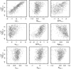 |
Fig. 10. LyC escaping luminosity vs. each of the nine galaxy variables. All variables plotted here are scaled (as denoted by the subscript s) using Eq. (4), as described in Sect. 4.1.2. The particular definitions of the parameters are as follows: |

4.1.3. Estimating the quality of the fit
There are several metrics that can be used to quantify how suitable the model is or how well it fits the data. A popular statistical metric for the multivariate regression model is the R2, which is a measure of how much of the response variance is explained by the model (i.e., the linear combination of the predictors). It is mathematically defined as
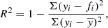 (5)
(5)
where yi is the actual y value (i.e., the y value from our simulation of the i-th halo),  is the mean value of these y values, and fi is the predicted value for the i-th halo computed using the model. An R2 = 0 means that the model explains no response variance, and R2 = 1 means that the model explains all the response variance (i.e., it can predict y exactly). So the closer the R2 value is to 1, the better the model.
Although R2 is a widely used metric of model performance, it should be noted that the value of R2 always increases, however slightly, when more and more variables are added to the model. Therefore, in models where the number of x variables is large, R2 may slightly overestimate the model performance. To ensure that our metric does not depend on the number of x variables, we define the adjusted  as
as
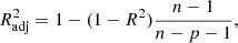 (6)
(6)
where n is the number of data points (galaxies) and p is the number of x variables in the model (see, e.g., Feigelson & Babu 2012). The adjusted R2 increases only when the addition of a x variable increases the R2 more than it would just by chance. The value of  will always be equal to or less than R2. From here onward, whenever we mention R2 and its values, either in text or in figures, we mean the
  , unless otherwise specified.
4.1.4. Finding the most important predictors
We performed a stepwise forward and backward selection method to determine which x variables are the most important for predicting y. In forward selection, the model takes the x variables one by one, inspects them to determine which one of them leads to the largest value of R2 by itself, and classifies that as the most important x variable (rank 1). Then the model adds each of the remaining x variables one by one to rank 1, and the variable that produces the largest increase in R2 value is the second most important x variable (rank 2). This continues until all the variables have been added and a ranked choice of x variables has been made. In the backward selection method, the model starts with all x variables and then determines which one variable removal decreases the value of R2 the least, this is least important variable. The process continues until all but one variable have been removed and a ranking has been generated. We use both methods on our data set.
4.1.5. Validating the models
After building the regression models, it is important to estimate the performance of the model on various data sets. To do so, we used the repeated k-fold cross-validation method to test the model performance. First, the entire data set was randomly divided into k subsets, where the number k (typically 5 or 10) can be specified. Then we reserved one subset as test data and estimated the model using the rest of the subsets, which act as training data. We then used this estimated model on the test data in order to calculate the fit/error indicators (which can be  , the root-mean-square estimate, or the mean absolute error). We repeated this process k times and ensured that each of the subsets acted as the test data set once. Then we calculated the average of these indicators from these k measurements of errors. This whole process of dividing the full data set into test-train data sets and computing the average indicators was then performed multiple times, and finally we averaged all the indicators corresponding to each model and compared the average value with the
  of the full model.
4.2. Application to SPHINX galaxies
From Eq. (3) we can deduce that the multivariate linear model is suitable if some (or all) x variables individually vary linearly with y (i.e., if at least for some variables y ∝ xn). If none of the x variables have any linear correlation with y, it is unlikely that a linear combination of them can determine y. Therefore, we first explore if individual correlation between y and any x variable exists.
Such an exploratory plot in shown in Fig. 10 where we plot the response variable  versus each of the galaxy properties. From this figure we find that
  correlates well with
  and SFR, along with some other weaker correlations. Similar plot for
  and
and  is provided in appendix (Figs. A.6 and A.7) where we see that
  is strongly correlated to SFR and
  and weakly correlated to mass and stellar age and
  is correlated to
  . This preliminary inspection shows that a multivariate linear regression can be a good model for predicting LyC.
4.2.1. Sample selection
Before we delve into regression modeling, we examine the galaxy data set to select a galaxy sample that can be used for building the model. The initial data set contains 1933 galaxies, which is the sample of all galaxies with stellar mass ≥106 M⊙ at z = 6, 7, 8, 9, and 10 (Sect. 2.2).
As discussed above and from Fig. A.6 it is clear that the SFR, especially recent (over last 10 Myr) SFR or SFR10, has a strong linear correlation with intrinsic LyC luminosity, and it is also correlated well with the escaping luminosity of LyC (Fig. 10). This is also expected from theoretical studies (Stanway et al. 2016; Raiter et al. 2010; Schaerer 2003; Partridge & Peebles 1967) that show star formation is the main driver for the production of both Lyα and LyC photons. In our data set, there are some galaxies (943 out of 1933, most of which are faint LAEs) that have no recent star formation (i.e., the average SFR over the last 10 Myr is SFR10 = 0; Fig. 4, right panel). So, when building our models we excluded these non-star-forming galaxies, and with this criterion there are 990 galaxies left in our data set.
Next we investigate this modified data set (galaxies with nonzero SFR) for any significant outliers. We find that there are some clear outliers in the distribution of  with values as low as 10−20. We remove galaxies with
  from the data set, after which the
  distribution is free of outliers. This leads to a data set of 940 galaxies. We find no significant outliers in other galaxy properties. Incidentally, we note that all of the galaxies in this final data set of 940 galaxies have both intrinsic and escaping Lyα luminosities > 1038 erg s−1.
4.2.2. Building the models and the most important variables
Our main goal is to predict the LyC luminosities and  using other properties. However, for many galaxies at high redshift the observation of Lyα luminosity can also be difficult, owing to increasing IGM opacity. Moreover, estimation of the intrinsic Lyα luminosity and hence
  is also challenging at all redshifts as these are not observables and must be derived using stellar models, which can have many underlying assumptions. So it can be useful to also build models for predicting these Lyα emissivities, which may complement existing methods.
Therefore, we explore the full predictive power of multiple linear regression models with our data set and we aim to build models to predict the following six quantities:  ,
,  ,
,  ,
,  ,
,  , and
, and  .
.
We investigate several combinations of physical parameters that we can access in the simulation to build a good predictive model. We calculate the performances of these models using the metric  and our most relevant model results are summarized in Table 2.
 for predicting different variables with different models.
Model 1. In Model 1, as predictors we supply all physical galaxy properties (GP), that is, items 1–8 from our list in Sect. 4.1.1, namely gas mass, stellar mass, galaxy radius, SFR10, SFR100, stellar age, stellar, and gas metallicity. We find that given only the physical properties of galaxies, we can predict the intrinsic LyC luminosity quite accurately (R2 = 0.87) but the emerging luminosity and the escape fraction cannot be modeled very well (R2 = 0.53 and 0.26, respectively). Conversely, both Lyα intrinsic (R2 = 0.88) and escaping (R2 = 0.71) luminosities can be predicted quite well with galaxy properties.
Model 2. When we add Lyα escaping luminosity to our input list of predictors (Model 2 in Table 2) we find that, in addition to the intrinsic luminosities, now the LyC escaping luminosity is also predicted with high accuracy, with R2 = 0.85. The average error in predicting the  , the root mean square error (RMSE; i.e., the average difference between the predicted and actual value), is approximately ∼4 (RMSE = 0.62 in log scale, Fig. 11). Both
  and
and  are also fairly well predicted with this model, with an R2 value of 0.69 and 0.64, respectively.
 |
Fig. 11. Prediction of intrinsic luminosity, escaping luminosity, and escape fraction of LyC from Model 2, where the input variables are the physical galaxy properties and the escaping Lyα luminosity. The R2 value for each fitting is noted in the plots. The red lines show the 1:1 correlation, or y = x line. The pink lines show the 95% prediction interval, and the blue lines show the 95% confidence interval. |
We consider Model 2 as our fiducial model and we show the predicted intrinsic and escaping LyC luminosities and  from Model 2 in Fig. 11 against the observed values from the simulation. In each of these plots we also show the 95% confidence interval and the 95% prediction interval. The confidence interval signifies that, given a set of predictor values (i.e., x values), the mean of the response variable will fall within this interval with 95% confidence. On the other hand, the prediction interval tells us where the next individual y value will fall. Given a set of x values, an individual y value will fall within the predictor interval with 95% confidence. The prediction interval accounts for both the uncertainty of the estimation of population mean as well as the variation in the individual y values. Hence, the predictor interval is always wider than the confidence interval. We see in Fig. 11 that most of the observed (in our simulation) values of y do indeed lie within the 95% predictor interval of our model.
Figure 11 shows both intrinsic and escaping luminosities are well predicted. We give here the equation for predicting  obtained using this model:
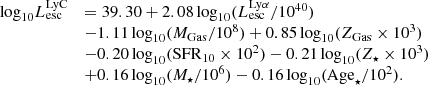 (7)
(7)
Here the luminosity is in erg s−1, mass is in M⊙, the SFR unit is M⊙ yr−1, stellar age is in Myr, and the metallicity unit is solar metallicity.
Here we note that in our models we included both the gas mass and the gas metallicity. Since the dust content is modeled by using these factors (as described in Sect. 2.4), including the dust in addition to the other parameters does not give us additional information (we tested this and found that inclusion of dust changes the  by less than 0.01%).
Most important variables. In the models described above, we supplied seven or eight galaxy properties for predicting various Lyα and LyC quantities. However, observing and determining many galaxy properties at high redshift can be extremely challenging. Thus, it is necessary to identify which of the x variables is the most important in predicting y. Here we discuss the ranking of most important predictors in the context of Model 2 and the response variables  ,
,  and
and  .
.
We present the results of the ranking process described in Sect. 4.1.4 in Table 3, listing the most important variables with their ranks and their  value. The
  value associated with the n-th rank variable is the
  the model produces including the first to n-th rank variable. The adjusted R2 increases only when the addition of a x variable increases the R2 more than it would be just by chance; otherwise, it actually decreases with variable addition (Sect. 4.1.3). In a ranking table, such as Table 3, when the adjusted R2 reaches a peak value, the model has reached its best predictive power. We perform both stepwise forward selection and backward selection for the ranking (Sect. 4.1.4), and find that both processes give the same ranking in all cases, which suggests that our ranking is stable.
Most important variables for predicting LyC luminosities and escape fractions using Model 2 ( ).
).
We find that 88% of the variance in  can be explained if we only use SFR10 and
  , meaning that these two values alone can provide a reliable prediction of the intrinsic ionizing power of galaxies. For escaping LyC, knowing the escaping Lyα luminosity is the most important factor and combining this with gas mass, gas metallicity and SFR10 can account for 85% of the variance. Lastly, the most important three predictors of
  are
are  , SFR10 and gas mass, as these three can explain 63% of the response variance. In the case of
  , variables with rank 1–6 increase the
  (up to 0.6569), but the addition of more properties decreases the model performance. Similarly, we find that in models for predicting
  , galaxy radius (rank 9) and for predicting
  , SFR100 and radius (rank 8 and 9) are not important.
4.2.3. Minimal model
Going one step further, we note that it is extremely difficult to observe gas properties in reionization era galaxies. Among the rest of the predictors used in our models so far, the observed LCEs we discuss in Sect. 3.1 and listed in Table 1 have only three predictors available, namely  , SFR10, and M⋆. It is now interesting to explore if a model built with only these three predictors can predict LyC quantities. We build a minimal model with these three predictors only (Model 3) and list the resulting model performances in Table 4. We find that here also
  is predicted with a high accuracy, R2 = 0.80 and the average error is a factor of RMSE ∼ 5.24. The intrinsic luminosities are also predicted very well, with fair performances for escape fractions. The equation for
  we get with this model is
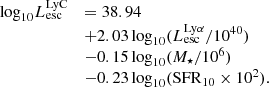 (8)
(8)
R2 for predicting different variables with the minimal model (Model 3).
The equation for  from this model can be written as
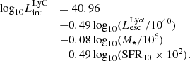 (9)
(9)
The units of the quantities are the same as described in Sect. 4.2.2. The ranking of the most important predictors for  with this minimal model is shown in Table 5, where we find that
  has rank 1, followed by SFR10 and M⋆, the same results we found with Model 2 (Sect. 4.2.2).
Most important variables for predicting  with the minimal model (Model 3).
4.3. Fitting the model to observed data
Finally, we explore if such a model can be fitted to real observed data. We list the properties of known Lyα and LyC emitters in Table 1. These galaxies have observations of their stellar mass, SFR, Lyα luminosity and their LyC luminosity at 900 Å. As discussed in Sect. 3.3 and shown in Fig. 3 these observed LCEs are more massive, have higher SFR and they are brighter in Lyα and LyC than the SPHINX galaxies. They are also observed at low redshifts, z ≤ 0.45 whereas the SPHINX galaxies are at z = 6−10. The simulated luminosities and escape fractions are angle-averaged quantities whereas observations are, of course, directional (further discussion in Sect. 5). Nevertheless, this is the only observed sample we currently have with both LyC and Lyα observations, so we evaluate our predictive model on these galaxies.
Since the observed galaxies have only three predictors available, we use our our minimal model (Model 3) described in Sect. 4.2.3 and use Eq. (8) for predicting the  of these observed LCEs. In Fig. 12 we show the predicted
  from this model versus the LyC luminosity that is derived from observations of
  (by multiplying the observed
  with a factor of 1434, the median value of the ratios
  /
/ derived from our simulation, Sect. 3.3). We find that the predicted luminosities are generally close to the observed values. In some cases the model over predicts the escaping luminosity, probably due to the differences in the physical properties between these observations and the SPHINX galaxy sample. Models performs best when the given input properties are inside the range of the training data (the ranges of properties for our SPHINX sample are shown in Fig. A.5), otherwise it needs to be extrapolated. The outlier with low predicted LyC is the galaxy Haro 11, which is located at z = 0.021, much closer than other observations; this may affect the galaxy properties.
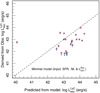 |
Fig. 12. Predicted |


4.4. Cross-validation of the models
We built these models using all 940 eligible galaxies available in our simulation data set. To check the model validity, we need to estimate the accuracy of these models when applied to other, new data that are not part of the data set used in building the models. The most straightforward way to do this is to apply this model to other new data sets where all of our desired input and output variables are available in order to readily test the difference between the prediction from models and the actual values. However, such full data sets can only be obtained from high resolution reionization simulations and currently we do not have other data sets. Instead, we can use repeated k-fold cross-validation method (described in Sect. 4.1.5) to gauge the performance of our models.
In this work we have used k = 10, so we divided the data set into ten random subsets and calculated the average  for our response variables. We repeated this process three times and get an average of
  from these runs. We calculated the k-fold
  for each model and have found that the
  from the k-fold test is always very similar to the
  we calculated when building the model with our whole data set. For example, when we performed the cross-validation for Model 2, for predicting
  ,
,  , and
, and  we get an average
  of 0.8996, 0.8945, and 0.8471, respectively, compared to 0.9006, 0.8956, and 0.8466 from our full model, as shown in Table 2. These respective
  values are very close to one another, which shows that our proposed models are indeed stable.
5. Discussion
In this study we have explored the relationship between Lyα and LyC emission from simulated EoR galaxies, and we have shown that it is possible to predict LyC emission of galaxies using their physical and Lyα properties. However, there are some important limitations of this study that we discuss below.
Limitations of the simulation. Our simulation has a box size of 10 Mpc, and the most luminous LAE in our sample of 1933 galaxies has a luminosity of 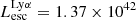 erg s−1. As we have discussed in Sect. 3.3 and shown in Figs. 4 and 5, recent observations of MUSE LAEs and low-redshift LyC leakers (Table 1) are starting to overlap with the brightest end of our sample of simulated galaxies. However, our sample is at z ≥ 6, and at these very high redshifts, the lower limit of observed Lyα luminosity is around ∼1043 erg s−1, still more luminous than our brightest galaxies. These detections are probably not representative of the underlying LAEs populations. Although they may play a central role in reionizing the Universe, as demonstrated by the recent discovery of an extremely bright LCE at z ∼ 3 (Marques-Chaves et al. 2021), the lack of very bright LAEs in our sample prevents us from making quantitative predictions for the contribution of very bright LAEs to reionization. As a consequence, our estimate of the fraction of the ionizing photon budget provided by galaxies with
  erg s−1 in Sect. 3.7 could well be a lower limit. In order to directly compare our predictions with observational data and to make better statistical predictions for bright galaxies, we need to analyze more luminous galaxies, for which we need to simulate a larger volume. The next generation of SPHINX will simulate a volume eight times larger than in the current study (i.e., 20 cMpc in width), which will include halos with stellar masses (virial masses) of up to about 1010 M⊙(1011 M⊙) at z = 6.
IGM attenuation. In this work we have not considered the effects of the IGM absorption. The IGM is an important factor in determining the observability of Lyα emission at these high redshifts because, for LAEs to be observable, Lyα must be transmitted through a partially neutral IGM, which can easily scatter Lyα photons off the line of sight. This can considerably reduce the visibility of LAEs during the EoR, as hinted at by the drop in the LAE fraction at z > 6 (Schenker et al. 2014; Kusakabe et al. 2020; Garel et al. 2021). Our results in this paper depict both Lyα and LyC luminosities as they would be observed just outside of the halo virial radius. In practice, some correction for the IGM can be applied to the data before applying our model to estimate the  of galaxies. Furthermore, the absence of IGM absorption allowed us to compare our simulation results to low-redshift observations of LCEs. For more realistic modeling and a direct comparison with high-redshift observations, we need to consider IGM absorption. Garel et al. (2021) predicts that the IGM transmission in Sphinx decreases from a factor of ∼2 at z = 6 to ∼10 at z = 9. Nevertheless, this study is the first necessary step to assess the link between Lyα and LyC escape from galaxies. Since there are known LAEs at z > 6 (e.g., Meyer et al. 2021 and references therein), depending on the topology of the reionization, Lyα emission may still go through large ionized bubbles at high redshift (Dijkstra 2014; Mason & Gronke 2020; Gronke et al. 2021), and could serve as a tracer for LyC escape from galaxies at the cosmic dawn.
Directional variation. In this study we chose to consider global, theoretical estimates of the Lyα and LyC quantities since they are the quantities that matter when determining the ionizing photon budget and studying the process of reionization.
However, when we observe galaxies we will, of course, only be able to observe them from one direction (along our line of sight). Furthermore, the Lyα and LyC luminosities and escape fraction of the same galaxy can differ significantly from direction to direction (Cen & Kimm 2015; Mauerhofer et al. 2021; Chuniaud et al., in prep.). To capture this added complexity, we will need to conduct a directional analysis of our galaxies. As a first attempt to quantify the angular variations in Lyα and LyC luminosities escaping from our simulated galaxies, we imagine a sphere around a halo at the halo virial radius and divide the surface area of the sphere into 1728 equal area pixels. We then count the Lyα and LyC photons that escape each of these pixels and calculate the  and
and  through each of them. For each pixel direction then we have the directional luminosity (
 ). In Fig. 13 we show the distribution of the directional Lyα and LyC luminosities (1728 directions for each galaxy) of the 674 sphinx galaxies (all galaxies at z = 6 snapshot) as a function of their actual global luminosities. Interestingly, we find that Lyα-bright galaxies can vary up to a factor of ∼100 compared to their angle-averaged
  , whereas faint galaxies are more isotropic. On the other hand, the directional LyC luminosities vary quite a lot at all angle-averaged LyC luminosities. As we discussed in Sect. 3.5, Lyα photons can scatter numerous times before escaping; hence, they have a higher chance of finding channels in the ISM with low column density and their directional distribution is generally more isotropic. Conversely LyC photons generally escape close to the galaxy center where they are mainly produced, so they have lower probabilities of finding many channels, which can result in a more anisotropic distribution of directional luminosities.
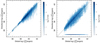 |
Fig. 13. Directional Lyα and LyC emission from galaxies vs. their global luminosities. Left: directional |


The broad variety of Lyα spectral shapes and strengths observed from galaxies is also one of the main probes of strong directional variations. Indeed, several recent observational studies (Verhamme et al. 2017; Steidel et al. 2018; Izotov et al. 2021) have found that spectral features of Lyα line profiles, such as high rest-frame equivalent widths and a narrow separation between the blue and red peak of Lyα spectra, correlate positively with escape of LyC. Testing these directional spectral features are beyond the scope of this article. But these two approaches are complementary of each other and we would ideally need both to get a complete picture of the contribution of the galaxies along our line of sight, and globally, to the reionization process. To that end, in the next step, we employ peeling-off algorithms on our galaxies and observe them from several directions. Then we can build mock observations to compare directly with existing and future observations and comment on how to employ our predictive models based on observed directional properties.
Uncertainties in the intrinsic LyC spectral distributions. The shape of the ionizing spectrum of galaxies is still poorly constrained. The LCEs detected so far have all been observed close to the Lyman limit (e.g., Steidel et al. 2018; Izotov et al. 2021; Flury et al. 2022). The only exception is the recent discovery of a z ∼ 1.4 galaxy leaking ionizing radiation at 600 Å rest-frame with the Astrosat (Saha et al. 2020). The theoretical predictions from population synthesis models is also a debated topic so far. The SPHINX simulation uses BPASS models (Stanway et al. 2016) to build the spectral energy distributions of galaxies, and in this version of SPHINX, all stars are binary systems. The binary star systems can emit more LyC photons for a longer time compared to single stellar populations, which impacts the full reionization history (Rosdahl et al. 2018). While binaries appear as a central ingredient in stellar radiation modeling at the EoR, the fraction of binary stars in the early Universe remains uncertain, as well as their exact spectral contribution.
While discussing the relationship of Lyα and LyC intrinsic luminosities in Sect. 3.3, we noted that galaxies (77/1933 or 3.98% of the population) at the very faint end of Lyα ( erg s−1) have LyC luminosity in the range of 1038 − 1040 erg s−1 (see Fig. 5). These faint LAEs are extremely gas deficient compared to the rest of the population, as shown in Fig. 14. So we find that in these systems there is not enough gas in the ISM to produce Lyα photons, resulting in very low
  . In contrast, these galaxies do have some residual LyC production although there have been no star formation in them in the last 10 Myrs (i.e., SFR10 = 0). We show the stellar ages of these systems in Fig. 14 and find that their median ages range from 100–300 Myrs and even their minimum stellar ages are very high. Furthermore, in all of them the 25th, 50th, and 75th percentile of ages are very close in values. This indicates that these systems are very old and their star formation finished within a short amount of time. Stanway et al. (2016; Fig. 1) demonstrates that, for binary populations in BPASS models with an instantaneous star formation model, it is possible for stellar populations to emit ∼1049 LyC photons/s at an age of 100 Myr. So in these faint LAEs, it is feasible that even though the galaxies have very old stellar systems, the LyC production is non-negligible. If these simulated galaxies exist in the real Universe, their LyC contribution to the reionization photon budget cannot be captured by their Lyα emission, and they will be missed by our prediction models.
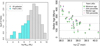 |
Fig. 14. Gas content and stellar age of faint LAEs. Left: distribution of gas mass in the faint LAEs ( |

6. Summary
We explore the connection between LyC and Lyα emission from EoR galaxies using a sample of 1933 simulated galaxies in the SPHINX RHD simulation. We post-process these galaxies using the radiative transfer code RASCAS to obtain their Lyα emission properties.
We first investigate the link between Lyα and LyC radiation from galaxies, and our main results are as follows:
-
The intrinsic Lyα and LyC luminosities are strongly correlated. The total escaping LyC (0–912 Å) luminosities are also correlated with escaping Lyα luminosity, although the dispersion is higher, especially in faint LAEs.
-
Given a threshold in observed LyC luminosity, as galaxies become brighter in Lyα, the fraction of observable LCEs among the LAE samples increases.
-
In bright LAEs (
 erg s−1), escape fractions of Lyα and LyC are correlated and in good agreement with the observed LCEs. However, when we consider all galaxies, including the fainter ones, there is no correlation, which suggests that the observed correlation is likely a selection effect.
 -
The median
 of galaxies gradually decreases with their Lyα luminosity and at the bright end with
  erg s−1; the median
  . The median value of
  is low for all Lyα luminosities, with the bright LAEs (
 erg s−1) having a median
  .
. -
Although very faint galaxies are more numerous, the relatively bright LAEs contribute more to reionization. In our SPHINX volume, LAEs with
 erg s−1 account for about 90% of the total ionizing luminosity in the simulation box, even though they are only 6.8% of the population.
We explored models for predicting LyC emission from galaxies using their physical and Lyα properties. We applied multivariate linear models to our sample of simulated galaxies, and the main results are summarized below:
-
We built a set of models using different sets of galaxy properties as input parameters and predicted LyC luminosities and escape fractions. In our fiducial model (Model 2), we give eight physical galaxy properties (gas mass, stellar mass, galaxy Rvir, SFR10, SFR100, stellar age, and stellar and gas metallicity) and
 as input parameters. The resulting model can predict
  and
and  very well, with high (adjusted) R2 values of 0.8969 and 0.8516, respectively. The
  is also predicted fairly well.
 -
We also determined the most important input variables for predicting LyC and find that the top four predictors of
 are
are  , gas mass, gas metallicity, and SFR10.
These results and the predictive models can be very useful in predicting the LyC emission from EoR galaxies and can thus help us determine the primary sources of reionization. We can apply these models to the upcoming EoR galaxy observations of JWST and other future surveys. They can also facilitate the selection and detection of LyC leakers. These models can be helpful for planning future direct LCE observation missions at lower redshifts. In a future work, we will investigate the effect of the directional variation in Lyα and LyC escape from galaxies, as well as IGM attenuation, on our predictions.
After reionization, the Universe has stayed ionized, so the local Universe LyC photons can travel without being absorbed, unlike in high z where neutral hydrogen atoms can absorb them easily.
Acknowledgments
We thank the anonymous referee for valuable comments and suggestions that have substantially improved the paper. MM, AV and TG are supported by the ERC Starting grant 757258 ‘TRIPLE’. AV acknowledges support from SNF Professorship PP00P2_176808. TK was supported by the National Research Foundation of Korea (NRF-2019K2A9A1A0609137711 and NRF-2020R1C1C1007079). We have performed the radiative transfer calculations in the LESTA and BAOBAB high-performance computing clusters of University of Geneva, and the RT post-processing for 1933 halos took approximately ∼37 000 CPU hours. The SPHINX simulation results of this research have been achieved using the PRACE Research Infrastructure resource SuperMUC based in Garching, Germany, under PRACE grant 2016153539. We additionally acknowledge support and computational resources from the Common Computing Facility (CCF) of the LABEX Lyon Institute of Origins (ANR-10-LABX-66).
References
- Aubert, D., Pichon, C., & Colombi, S. 2004, MNRAS, 352, 376 [Google Scholar]
- Bacon, R., Brinchmann, J., Richard, J., et al. 2015, A&A, 575, A75 [NASA ADS] [CrossRef] [EDP Sciences] [Google Scholar]
- Bassett, R., Ryan-Weber, E. V., Cooke, J., et al. 2019, MNRAS, 483, 5223 [Google Scholar]
- Behrens, C., & Braun, H. 2014, A&A, 572, A74 [NASA ADS] [CrossRef] [EDP Sciences] [Google Scholar]
- Cantalupo, S., Porciani, C., & Lilly, S. J. 2008, ApJ, 672, 48 [Google Scholar]
- Cen, R., & Kimm, T. 2015, ApJ, 801, L25 [Google Scholar]
- Chisholm, J., Orlitová, I., Schaerer, D., et al. 2017, A&A, 605, A67 [NASA ADS] [CrossRef] [EDP Sciences] [Google Scholar]
- Cowie, L. L., Barger, A. J., & Trouille, L. 2009, ApJ, 692, 1476 [NASA ADS] [CrossRef] [Google Scholar]
- Dijkstra, M. 2014, PASA, 31, e040 [Google Scholar]
- Dijkstra, M., Gronke, M., & Venkatesan, A. 2016, ApJ, 828, 71 [Google Scholar]
- Drake, A. B., Garel, T., Wisotzki, L., et al. 2017, A&A, 608, A6 [NASA ADS] [CrossRef] [EDP Sciences] [Google Scholar]
- Erb, D. K. 2015, Nature, 523, 169 [Google Scholar]
- Erb, D. K., Bogosavljević, M., & Steidel, C. C. 2011, ApJ, 740, L31 [NASA ADS] [CrossRef] [Google Scholar]
- Faucher-Giguère, C.-A. 2020, MNRAS, 493, 1614 [Google Scholar]
- Faucher-Giguère, C.-A., Kereš, D., Dijkstra, M., Hernquist, L., & Zaldarriaga, M. 2010, ApJ, 725, 633 [Google Scholar]
- Feigelson, E. D., & Babu, G. J. 2012, Modern Statistical Methods for Astronomy: With R Applications (Cambridge University Press) [CrossRef] [Google Scholar]
- Finkelstein, S. L., Papovich, C., Dickinson, M., et al. 2013, Nature, 502, 524 [CrossRef] [Google Scholar]
- Flury, S. R., Jaskot, A. E., Ferguson, H. C., et al. 2022, ApJS, 260, 1 [NASA ADS] [CrossRef] [Google Scholar]
- Fontanot, F., Cristiani, S., & Vanzella, E. 2012, MNRAS, 425, 1413 [Google Scholar]
- Fontanot, F., Cristiani, S., Pfrommer, C., Cupani, G., & Vanzella, E. 2014, MNRAS, 438, 2097 [Google Scholar]
- Garel, T., Blaizot, J., Rosdahl, J., et al. 2021, MNRAS, 504, 1902 [NASA ADS] [CrossRef] [Google Scholar]
- Gazagnes, S., Chisholm, J., Schaerer, D., Verhamme, A., & Izotov, Y. 2020, A&A, 639, A85 [NASA ADS] [CrossRef] [EDP Sciences] [Google Scholar]
- Goerdt, T., Dekel, A., Sternberg, A., et al. 2010, MNRAS, 407, 613 [Google Scholar]
- Gronke, M., Ocvirk, P., Mason, C., et al. 2021, MNRAS, 508, 3697 [NASA ADS] [CrossRef] [Google Scholar]
- Hayes, M., Östlin, G., Schaerer, D., et al. 2013, ApJ, 765, L27 [NASA ADS] [CrossRef] [Google Scholar]
- Heckman, T. M., Borthakur, S., Overzier, R., et al. 2011, ApJ, 730, 5 [Google Scholar]
- Henry, A., Scarlata, C., Martin, C. L., & Erb, D. 2015, ApJ, 809, 19 [Google Scholar]
- Inoue, A. K., Shimizu, I., Iwata, I., & Tanaka, M. 2014, MNRAS, 442, 1805 [NASA ADS] [CrossRef] [Google Scholar]
- Inoue, A. K., Hasegawa, K., Ishiyama, T., et al. 2018, PASJ, 70, 55 [Google Scholar]
- Itoh, R., Ouchi, M., Zhang, H., et al. 2018, ApJ, 867, 46 [NASA ADS] [CrossRef] [Google Scholar]
- Izotov, Y. I., Orlitová, I., Schaerer, D., et al. 2016a, Nature, 529, 178 [Google Scholar]
- Izotov, Y. I., Schaerer, D., Thuan, T. X., et al. 2016b, MNRAS, 461, 3683 [Google Scholar]
- Izotov, Y. I., Schaerer, D., Worseck, G., et al. 2018a, MNRAS, 474, 4514 [Google Scholar]
- Izotov, Y. I., Worseck, G., Schaerer, D., et al. 2018b, MNRAS, 478, 4851 [Google Scholar]
- Izotov, Y. I., Worseck, G., Schaerer, D., et al. 2021, MNRAS, 503, 1734 [NASA ADS] [CrossRef] [Google Scholar]
- Jaskot, A. E., & Oey, M. S. 2013, ApJ, 766, 91 [Google Scholar]
- Jung, I., Finkelstein, S. L., Dickinson, M., et al. 2019, ApJ, 877, 146 [CrossRef] [Google Scholar]
- Katz, H., Galligan, T. P., Kimm, T., et al. 2019, MNRAS, 487, 5902 [NASA ADS] [CrossRef] [Google Scholar]
- Katz, H., Ďurovčíková, D., Kimm, T., et al. 2020, MNRAS, 498, 164 [Google Scholar]
- Kimm, T., Blaizot, J., Garel, T., et al. 2019, MNRAS, 486, 2215 [Google Scholar]
- Konno, A., Ouchi, M., Ono, Y., et al. 2014, ApJ, 797, 16 [Google Scholar]
- Kulkarni, G., Worseck, G., & Hennawi, J. F. 2019, MNRAS, 488, 1035 [Google Scholar]
- Kusakabe, H., Blaizot, J., Garel, T., et al. 2020, A&A, 638, A12 [NASA ADS] [CrossRef] [EDP Sciences] [Google Scholar]
- Laursen, P., Sommer-Larsen, J., & Andersen, A. C. 2009, ApJ, 704, 1640 [Google Scholar]
- Laursen, P., Sommer-Larsen, J., Milvang-Jensen, B., Fynbo, J. P. U., & Razoumov, A. O. 2019, A&A, 627, A84 [NASA ADS] [CrossRef] [EDP Sciences] [Google Scholar]
- Leitet, E., Bergvall, N., Piskunov, N., & Andersson, B. G. 2011, A&A, 532, A107 [NASA ADS] [CrossRef] [EDP Sciences] [Google Scholar]
- Leitet, E., Bergvall, N., Hayes, M., Linné, S., & Zackrisson, E. 2013, A&A, 553, A106 [NASA ADS] [CrossRef] [EDP Sciences] [Google Scholar]
- Loeb, A., & Barkana, R. 2001, ARA&A, 39, 19 [NASA ADS] [CrossRef] [Google Scholar]
- Madau, P. 1995, ApJ, 441, 18 [NASA ADS] [CrossRef] [Google Scholar]
- Marques-Chaves, R., Schaerer, D., Álvarez-Márquez, J., et al. 2021, MNRAS, 507, 524 [NASA ADS] [CrossRef] [Google Scholar]
- Mason, C. A., & Gronke, M. 2020, MNRAS, 499, 1395 [Google Scholar]
- Matthee, J., Sobral, D., Darvish, B., et al. 2017, MNRAS, 472, 772 [Google Scholar]
- Matthee, J., Sobral, D., Gronke, M., et al. 2018, A&A, 619, A136 [NASA ADS] [CrossRef] [EDP Sciences] [Google Scholar]
- Matthee, J., Pezzulli, G., Mackenzie, R., et al. 2020, MNRAS, 498, 3043 [Google Scholar]
- Mauerhofer, V., Verhamme, A., Blaizot, J., et al. 2021, A&A, 646, A80 [NASA ADS] [CrossRef] [EDP Sciences] [Google Scholar]
- Meyer, R. A., Laporte, N., Ellis, R. S., Verhamme, A., & Garel, T. 2021, MNRAS, 500, 558 [Google Scholar]
- Michel-Dansac, L., Blaizot, J., Garel, T., et al. 2020, A&A, 635, A154 [EDP Sciences] [Google Scholar]
- Micheva, G., Zackrisson, E., Östlin, G., Bergvall, N., & Pursimo, T. 2010, MNRAS, 405, 1203 [NASA ADS] [Google Scholar]
- Nakajima, K., & Ouchi, M. 2014, MNRAS, 442, 900 [Google Scholar]
- Ocvirk, P., Gillet, N., Shapiro, P. R., et al. 2016, MNRAS, 463, 1462 [Google Scholar]
- Oesch, P. A., van Dokkum, P. G., Illingworth, G. D., et al. 2015, ApJ, 804, L30 [Google Scholar]
- Ono, Y., Ouchi, M., Mobasher, B., et al. 2012, ApJ, 744, 83 [Google Scholar]
- Östlin, G., Hayes, M., Duval, F., et al. 2014, ApJ, 797, 11 [CrossRef] [Google Scholar]
- Ouchi, M., Harikane, Y., Shibuya, T., et al. 2018, PASJ, 70, S13 [Google Scholar]
- Pardy, S. A., Cannon, J. M., Östlin, G., Hayes, M., & Bergvall, N. 2016, AJ, 152, 178 [NASA ADS] [CrossRef] [Google Scholar]
- Partridge, R. B., & Peebles, P. J. E. 1967, ApJ, 147, 868 [Google Scholar]
- Planck Collaboration XVI. 2014, A&A, 571, A16 [NASA ADS] [CrossRef] [EDP Sciences] [Google Scholar]
- Puschnig, J., Hayes, M., Östlin, G., et al. 2017, MNRAS, 469, 3252 [Google Scholar]
- Raiter, A., Fosbury, R. A. E., & Teimoorinia, H. 2010, A&A, 510, A109 [NASA ADS] [CrossRef] [EDP Sciences] [Google Scholar]
- Roberts-Borsani, G. W., Bouwens, R. J., Oesch, P. A., et al. 2016, ApJ, 823, 143 [NASA ADS] [CrossRef] [Google Scholar]
- Rosdahl, J., & Blaizot, J. 2012, MNRAS, 423, 344 [Google Scholar]
- Rosdahl, J., Blaizot, J., Aubert, D., Stranex, T., & Teyssier, R. 2013, MNRAS, 436, 2188 [Google Scholar]
- Rosdahl, J., Katz, H., Blaizot, J., et al. 2018, MNRAS, 479, 994 [NASA ADS] [Google Scholar]
- Runnholm, A., Hayes, M., Melinder, J., et al. 2020, ApJ, 892, 48 [NASA ADS] [CrossRef] [Google Scholar]
- Saha, K., Tandon, S. N., Simmonds, C., et al. 2020, Nat. Astron., 4, 1185 [NASA ADS] [CrossRef] [Google Scholar]
- Schaerer, D. 2003, A&A, 397, 527 [NASA ADS] [CrossRef] [EDP Sciences] [Google Scholar]
- Schaerer, D., Izotov, Y. I., Verhamme, A., et al. 2016, A&A, 591, L8 [NASA ADS] [CrossRef] [EDP Sciences] [Google Scholar]
- Schenker, M. A., Stark, D. P., Ellis, R. S., et al. 2012, ApJ, 744, 179 [Google Scholar]
- Schenker, M. A., Ellis, R. S., Konidaris, N. P., & Stark, D. P. 2014, ApJ, 795, 20 [NASA ADS] [CrossRef] [Google Scholar]
- Shibuya, T., Kashikawa, N., Ota, K., et al. 2012, ApJ, 752, 114 [Google Scholar]
- Shibuya, T., Ouchi, M., Konno, A., et al. 2018, PASJ, 70, S14 [Google Scholar]
- Smith, A., Ma, X., Bromm, V., et al. 2019, MNRAS, 484, 39 [NASA ADS] [CrossRef] [Google Scholar]
- Song, M., Finkelstein, S. L., Livermore, R. C., et al. 2016, ApJ, 826, 113 [NASA ADS] [CrossRef] [Google Scholar]
- Songaila, A., Hu, E. M., Barger, A. J., et al. 2018, ApJ, 859, 91 [Google Scholar]
- Spitzer, L. 1978, Physical Processes in the Interstellar Medium (Wiley) [Google Scholar]
- Stanway, E. R., Eldridge, J. J., & Becker, G. D. 2016, MNRAS, 456, 485 [NASA ADS] [CrossRef] [Google Scholar]
- Stark, D. P. 2016, ARA&A, 54, 761 [Google Scholar]
- Stark, D. P., Ellis, R. S., Charlot, S., et al. 2017, MNRAS, 464, 469 [NASA ADS] [CrossRef] [Google Scholar]
- Steidel, C. C., Bogosavljević, M., Shapley, A. E., et al. 2018, ApJ, 869, 123 [Google Scholar]
- Teyssier, R. 2002, A&A, 385, 337 [CrossRef] [EDP Sciences] [Google Scholar]
- Trainor, R. F., Steidel, C. C., Strom, A. L., & Rudie, G. C. 2015, ApJ, 809, 89 [NASA ADS] [CrossRef] [Google Scholar]
- Trebitsch, M., Verhamme, A., Blaizot, J., & Rosdahl, J. 2016, A&A, 593, A122 [NASA ADS] [CrossRef] [EDP Sciences] [Google Scholar]
- Trebitsch, M., Dubois, Y., Volonteri, M., et al. 2021, A&A, 653, A154 [NASA ADS] [CrossRef] [EDP Sciences] [Google Scholar]
- Tweed, D., Devriendt, J., Blaizot, J., Colombi, S., & Slyz, A. 2009, A&A, 506, 647 [NASA ADS] [CrossRef] [EDP Sciences] [Google Scholar]
- Urrutia, T., Wisotzki, L., Kerutt, J., et al. 2019, A&A, 624, A141 [NASA ADS] [CrossRef] [EDP Sciences] [Google Scholar]
- Vanzella, E., Pentericci, L., Fontana, A., et al. 2011, ApJ, 730, L35 [NASA ADS] [CrossRef] [Google Scholar]
- Verhamme, A., Dubois, Y., Blaizot, J., et al. 2012, A&A, 546, A111 [NASA ADS] [CrossRef] [EDP Sciences] [Google Scholar]
- Verhamme, A., Orlitová, I., Schaerer, D., & Hayes, M. 2015, A&A, 578, A7 [NASA ADS] [CrossRef] [EDP Sciences] [Google Scholar]
- Verhamme, A., Orlitová, I., Schaerer, D., et al. 2017, A&A, 597, A13 [NASA ADS] [CrossRef] [EDP Sciences] [Google Scholar]
- Wise, J. H. 2019, Contemp. Phys., 60, 145 [NASA ADS] [CrossRef] [Google Scholar]
- Yajima, H., Li, Y., & Zhu, Q. 2013, ApJ, 773, 151 [NASA ADS] [CrossRef] [Google Scholar]
- Yajima, H., Li, Y., Zhu, Q., et al. 2014, MNRAS, 440, 776 [NASA ADS] [CrossRef] [Google Scholar]
- Yang, H., Malhotra, S., Gronke, M., et al. 2017, ApJ, 844, 171 [NASA ADS] [CrossRef] [Google Scholar]
- Zitrin, A., Labbé, I., Belli, S., et al. 2015, ApJ, 810, L12 [Google Scholar]
Appendix A: Supplementary figures
A.1. Comparing the z=6 sample to the stacked sample
In the main text, we combine our galaxy samples at different redshifts and explored the connection between LyC and Lyα emission from galaxies. Herein we inspect if the selected populations of galaxies at different redshifts have significantly different properties. We compare two samples specifically, 674 galaxies at z = 6, and the stacked sample of 1933 galaxies that combines all galaxies in all of the 5 redshifts (z = 6, 7, 8, 9, 10).
We compare the physical properties, Lyα properties and LyC properties of these two samples and present the results in Fig. A.1. In the top row, it shows comparisons of three physical galaxy properties, stellar mass, gas mass and SFR calculated over the last 10 Myrs (SFR10). We find that in each case, the distributions are very similar and the median value of the mass and SFR10 is also almost the same. We also compared the halo mass, the size of the galaxy (Rvir, gal) and halo (Rvir, halo), and the SFR calculated over the last 100 Myr (SFR100) and found that for each of these properties, the two samples have very similar values. Here we choose to show only the three properties mentioned as representative plots for brevity’s sake.
 |
Fig. A.1. Comparing the physical, Lyα, and LyC properties of galaxies of the stacked sample (gray) with the z=6 sample (blue). The top row compares stellar mass (left), gas mass (middle), and SFR10(right). The middle row compares the Lyα properties of the two samples with intrinsic luminosity (left), escaping luminosity (middle), and escape fraction (right). The bottom row shows the same properties but for LyC radiation. The dashed lines show the median value of the properties for both the stacked (black) and z = 6 sample (blue). |
In the second and third row of Fig. A.1, we have compared the Lyα and LyC properties of the two samples, showing for each intrinsic luminosity, escaping luminosity and the escape fraction. The plots clearly show that for both intrinsic and escaping luminosity, the distributions are again very similar with almost the same median values.
For  and
and  comparisons, we find that the distribution for either sample is not single peaked or Gaussian like the other properties. The
  distribution is close to a binomial with values biased toward close to either 0 or 1.
  distribution is also biased toward values close to 0.
Since a median of these two distributions would not be very meaningful, we calculate the percentage of the population that have very high  , defined as
  and find that in z = 6 sample 31% fall in this category, whereas in the stacked sample the population is 32%. For
  , the distribution peaks toward extremely low values, so we calculate the percentage of population with
  and find it to be 66.7% and 61% for the z = 6 and stacked sample, respectively. We find that the stacked sample is very similar to the z = 6 sample of galaxies and there are no large systematic differences between them in terms of their physical or radiative properties. We note that the age of the Universe at z = 6 is 927 Myr and at z = 10 it is 470 Myr, so between the redshift range of 6–10, only 457 Myr pass. So it is not surprising that we find the statistical properties of the galaxies within this time frame do not change significantly in our simulation. Our results suggest that we can use our stacked sample of 1933 galaxies for our Lyα and LyC analysis to study reionization era galaxies.
A.2. Contribution of recombination and collision to Lyα production
Figure A.2 shows the fraction of intrinsic Lyα that comes from recombination and collision, respectively. We find that in bright LAEs almost all of the  is generated from recombination. However, the contribution of collision becomes higher as galaxies becomes fainter. For example, in galaxies where
  erg s−1, collisions contribute a few percent, but this can rise to ∼50% in galaxies where
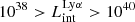 erg s−1.
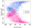 |
Fig. A.2. Fraction of intrinsic Lyα luminosity generated by recombination (blue) and collision (pink) as a function of |

A.3. Variation in escape fractions with escaping luminosities
We have discussed the relationship between Lyα and LyC luminosities and escape fractions in Appendix 3.3 and 3.5, respectively. Here we revisit them and discuss how galaxy escape fractions vary with their luminosities. In fig A.3 we show  as a function of their
  , similar to Fig 5, but here colored by their
  and
and  . We find that most of the galaxies have low
  and there is a clear trend that for a given
  , brighter LAEs have lower
  . When
  is high, most of the LyC is escaping, so there are few LyC photons available to produce Lyα; hence, Lyα luminosity is low. As
  decreases, more and more LyC photons are reprocessed into Lyα, and Lyα luminosity increases. On the other hand, most of the galaxies have high
  . In general, faint LAEs have high Lyα escape fraction, but there is significant scatter at each luminosities.
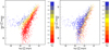 |
Fig. A.3. Escaping LyC luminosity of galaxies as a function of their escaping Lyα luminosity. This is the same as Fig 5, but the points here are colored by their |


A.4. Reionization accounting with lower mass limit
In Sect. 3.7 we have discussed the contribution of LAEs toward reionization and found that LAEs brighter than 1040 erg s−1 can account for 95% of the total ionizing luminosity in the simulation, suggesting that bright LAEs may be the most important sources of reionization. However, in this analysis, while counting the LyC contribution of LAEs, following our galaxy selection criterion in Sect. 2.2, we considered all galaxies with M⋆ > 106 M⊙. It will be instructive to explore how the results will change if we impose a lower mass limit, for example 105 M⊙. In order to investigate this, we need to first run the Lyα radiative transfer on all galaxies with M⋆ > 105 M⊙. Since the number of galaxies within 105 − 106 M⊙ range is very high, post-processing all of them in the full stacked sample will be very expensive. Hence, we limit our investigation to galaxies in z = 6 snapshot only. At z=6, there are 674 and 1495 galaxies with M⋆ > 106 M⊙ and M⋆ > 105 M⊙, respectively.
Similar to our analysis in Sect. 3.7, we first calculate the total LyC luminosity emitted by all (level 1) galaxies at z = 6. Then we calculate how much of this total LyC is emitted by galaxies with  > 1038, 1039, 1040, 1041 and 1042 erg s−1 using samples with both stellar mass limits of 106 and 105 M⊙. Figure A.4 show this cumulative fraction against the limiting Lyα luminosity of the galaxies. We find that LAEs brighter than 1040 erg s−1 can account for 95% of total LyC when counting only M⋆ > 106 M⊙ galaxies, and if we lower the mass limit to 105 M⊙, this fraction increases to 97%. At the low luminosity limit, LAEs brighter than 1038 erg/s contribute 97% (99%) of the re-ionizing radiation. This results show that although lowering the mass limit slightly increase these fractions, the differences are very small. This indicates that the reionization accounting we did in Sect. 3.7 with 106 M⊙ mass limit is reasonably accurate.
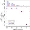 |
Fig. A.4. Fraction of the total escaping LyC luminosity emitted by galaxies brighter than a given Lyα luminosity limit as a function of the Lyα luminosity limit. Here we compare this fraction for two sets of galaxy samples: all galaxies at level 1 with M⋆ > 106 M⊙ (red points) and all galaxies at level 1 with M⋆ > 105 M⊙ (blue points). These galaxies are all taken from the z=6 snapshot. So, the denominator of the fraction is same in both cases: the total LyC emission from all galaxies (at level 1) at z = 6. The numerator calculates the total LyC luminosity of the galaxies brighter than a given Lyα luminosity limit with the two samples, for example the total LyC emitted by all galaxies (at level 1) with M⋆ > 106 (or 105) M⊙ and |


A.5. Multivariate model: More exploratory analysis
We show the histograms for the galaxy properties used in building our models (as listed in Sect. 4.1.1) for our sample of 940 galaxies (Sect. 4.2.1) in Fig. A.5. We discuss in Sect. 4.1 that before building a multivariate linear model to predict LyC properties, it is important to check if any of the proposed x variables or input variables have any correlation with the y variable or response variable. Figures A.6 and A.7 show such an exploratory plot of the response variable  and
and  versus various galaxy properties, respectively. We find that several properties, especially, SFR10 and
  , correlate very well with
  . There are also weak correlations with gas mass, SFR100, and stellar age. The
  is also correlated with
  . This all suggests that the multivariate linear regression model can be a good choice for predicting LyC emission from galaxies using these properties.
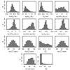 |
Fig. A.5. Histogram of the 14 galaxy properties (gas mass, stellar mass, galaxy radius, SFR10, SFR100, stellar age, stellar and gas metallicity, intrinsic and escaping luminosities, and escape fractions of Lyα and LyC, as described in Sect. 4.1.1) for our sample of 940 galaxies (Sect. 4.2.1) that were used to build the predictive models (Sect. 4.2.2). |
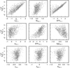 |
Fig. A.6.
|


All Tables
Most important variables for predicting LyC luminosities and escape fractions using Model 2 ().
All Figures
|
Fig. 1. Histograms of physical properties of the simulated galaxies in our sample. The histograms show the distribution of the stellar mass (left), gas mass (middle), and SFR10 (right) of the galaxies. The median values are shown by dashed black lines. The stellar mass histogram shows M⋆ within 30% of the halo virial radius. There are ten galaxies with M⋆ > 108 M⊙. The gas mass has a peaked distribution, with a few galaxies having very little gas (further discussion in Sect. 5). There are 943 galaxies with zero SFR10; these galaxies are represented in the bar at 10−6 (discussed in Sect. 4.2.1). |
| In the text | |
|
Fig. 2. Ratio of total intrinsic (left) and escaping (middle) LyC luminosity emitted over the range of 0–912 Å and the intrinsic and emitted LyC at 900 Å, as a function of their total escaping LyC luminosity. The median ratio calculated with all simulated galaxies is shown with the dashed red line. Some of the galaxies have |
| In the text | |
|
Fig. 3. Comparison of physical properties of observed LCEs (magenta points) and the simulated galaxies (black points). Here we show the stellar mass (top left), gas metallicity (oxygen abundances, i.e., 12 + log10(O/H) for observed galaxies, top middle), galaxy radius (galaxy virial radius for simulated ones and exponential disk scale length for observed ones, top right) and SFR (SFR10) as a function of their escaping Lyα luminosities. The Lyα luminosities of the SPHINX galaxies do not scale with stellar masses, metallicities, or galaxy sizes, whereas they do correlate with recent star formation, as expected. Top-right panel: we show the SFR (SFR10 for simulated galaxies) as a function of the stellar mass of galaxies. The properties of the observed LCEs are listed in Table 1, and more details can be found in their corresponding reference papers. |
| In the text | |
|
Fig. 4. Histograms of Lyα and LyC emission of our sample of 1933 galaxies. Top row: Lyα properties of our sample with intrinsic luminosity (left), escaping luminosity (middle), and escape fraction (right). Bottom row: same properties but for LyC radiation. In the middle panel of the top row, we also show the distribution of |
| In the text | |
|
Fig. 5. LyC luminosity of galaxies as a function of their Lyα counterparts. Left: intrinsic LyC luminosity of galaxies as a function of their intrinsic Lyα luminosity. The black and pink points show the total LyC luminosity (0–912 Å) and the 900 Å luminosity of the simulated galaxies, respectively (Sect. 3.1). The diamond-shaped magenta points show the observed LCEs described in Table 1. The sky blue points show the intrinsic luminosities derived from the analytic model described in this panel. Right: escaping LyC luminosity of galaxies as a function of their escaping Lyα luminosity. The solid yellow line shows the median |
| In the text | |
|
Fig. 6. Fraction of galaxies with |
| In the text | |
|
Fig. 7. Escape fractions of Lyα vs. LyC. The plots here show progressively brighter sample selection for all galaxies (top left) and galaxies with |
| In the text | |
|
Fig. 8. Median |
| In the text | |
|
Fig. 9. Total escaping ionizing luminosity of LAEs. Left: total escaping LyC luminosity of galaxies grouped by their Lyα luminosities as a function of their median Lyα luminosity. The histogram above shows the number of galaxies in the corresponding bins below. Right: conditional total escaping LyC luminosity of galaxies brighter than a given Lyα luminosity limit as a function of the Lyα luminosity limit. The histogram above indicates the number of galaxies where |
| In the text | |
|
Fig. 10. LyC escaping luminosity vs. each of the nine galaxy variables. All variables plotted here are scaled (as denoted by the subscript s) using Eq. (4), as described in Sect. 4.1.2. The particular definitions of the parameters are as follows: |
| In the text | |
|
Fig. 11. Prediction of intrinsic luminosity, escaping luminosity, and escape fraction of LyC from Model 2, where the input variables are the physical galaxy properties and the escaping Lyα luminosity. The R2 value for each fitting is noted in the plots. The red lines show the 1:1 correlation, or y = x line. The pink lines show the 95% prediction interval, and the blue lines show the 95% confidence interval. |
| In the text | |
|
Fig. 12. Predicted |
| In the text | |
|
Fig. 13. Directional Lyα and LyC emission from galaxies vs. their global luminosities. Left: directional |
| In the text | |
|
Fig. 14. Gas content and stellar age of faint LAEs. Left: distribution of gas mass in the faint LAEs ( |
| In the text | |
|
Fig. A.1. Comparing the physical, Lyα, and LyC properties of galaxies of the stacked sample (gray) with the z=6 sample (blue). The top row compares stellar mass (left), gas mass (middle), and SFR10(right). The middle row compares the Lyα properties of the two samples with intrinsic luminosity (left), escaping luminosity (middle), and escape fraction (right). The bottom row shows the same properties but for LyC radiation. The dashed lines show the median value of the properties for both the stacked (black) and z = 6 sample (blue). |
| In the text | |
|
Fig. A.2. Fraction of intrinsic Lyα luminosity generated by recombination (blue) and collision (pink) as a function of |
| In the text | |
|
Fig. A.3. Escaping LyC luminosity of galaxies as a function of their escaping Lyα luminosity. This is the same as Fig 5, but the points here are colored by their |
| In the text | |
|
Fig. A.4. Fraction of the total escaping LyC luminosity emitted by galaxies brighter than a given Lyα luminosity limit as a function of the Lyα luminosity limit. Here we compare this fraction for two sets of galaxy samples: all galaxies at level 1 with M⋆ > 106 M⊙ (red points) and all galaxies at level 1 with M⋆ > 105 M⊙ (blue points). These galaxies are all taken from the z=6 snapshot. So, the denominator of the fraction is same in both cases: the total LyC emission from all galaxies (at level 1) at z = 6. The numerator calculates the total LyC luminosity of the galaxies brighter than a given Lyα luminosity limit with the two samples, for example the total LyC emitted by all galaxies (at level 1) with M⋆ > 106 (or 105) M⊙ and |
| In the text | |
|
Fig. A.5. Histogram of the 14 galaxy properties (gas mass, stellar mass, galaxy radius, SFR10, SFR100, stellar age, stellar and gas metallicity, intrinsic and escaping luminosities, and escape fractions of Lyα and LyC, as described in Sect. 4.1.1) for our sample of 940 galaxies (Sect. 4.2.1) that were used to build the predictive models (Sect. 4.2.2). |
| In the text | |
|
Fig. A.6.
|
| In the text | |
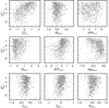 |
Fig. A.7. Same as A.6 but for the response variable |
| In the text | |
Current usage metrics show cumulative count of Article Views (full-text article views including HTML views, PDF and ePub downloads, according to the available data) and Abstracts Views on Vision4Press platform.
Data correspond to usage on the plateform after 2015. The current usage metrics is available 48-96 hours after online publication and is updated daily on week days.
Initial download of the metrics may take a while.