| Issue |
A&A
Volume 663, July 2022
|
|
|---|---|---|
| Article Number | A14 | |
| Number of page(s) | 24 | |
| Section | Planets and planetary systems | |
| DOI | https://doi.org/10.1051/0004-6361/202140543 | |
| Published online | 04 July 2022 | |
Detecting exoplanets with the false inclusion probability
Comparison with other detection criteria in the context of radial velocities
1
Observatoire Astronomique de l’Université de Genève,
Chemin de Pegasi 51 b,
1290
Versoix,
Switzerland
e-mail: This email address is being protected from spambots. You need JavaScript enabled to view it.
2
International Center for Advanced Studies (ICAS) and ICIFI (CONICET), ECyT-UNSAM,
Campus Miguelete, 25 de Mayo y Francia,
1650
Buenos Aires,
Argentina
3
Universidad de Buenos Aires, Facultad de Ciencias Exactas y Naturales,
Buenos Aires,
Argentina
4
CONICET – Universidad de Buenos Aires, Instituto de Astronomía y Física del Espacio (IAFE),
Buenos Aires,
Argentina
Received:
11
February
2021
Accepted:
12
May
2021
Abstract
Context. It is common practice to claim the detection of a signal if, for a certain statistical significance metric, the signal significance exceeds a certain threshold fixed in advance. In the context of exoplanet searches in radial velocity data, the most common statistical significance metrics are the Bayes factor and the false alarm probability (FAP). Both criteria have proved useful, but do not directly address whether an exoplanet detection should be claimed. Furthermore, it is unclear which detection threshold should be taken and how robust the detections are to model misspecification.
Aims. The aim of the present work is to define a detection criterion that conveys as precisely as possible the information needed to claim an exoplanet detection, as well as efficient numerical methods to compute it. We compare this new criterion to existing ones in terms of sensitivity and robustness to a change in the model.
Methods. We define a general detection criterion called the false inclusion probability (FIP). In the context of exoplanet detections it provides the posterior probability of presence of a planet with a period in a certain interval. Posterior distributions are computed with the nested sampling package POLYCHORD. We show that for FIP and Bayes factor calculations, defining priors on linear parameters as Gaussian mixture models can significantly speed up computations. The performance of the FAP, Bayes factor, and FIP are studied via simulations and analytical arguments. We compare the methods assuming the model is correct, then evaluate their sensitivity to the prior and likelihood choices.
Results. Among other properties, the FIP offers ways to test the reliability of the significance levels; it is a particularly efficient way to account for aliasing, and it allows the presence of planets to be excluded with a certain confidence. In our simulations, we find that the FIP outperforms existing detection metrics. We show that low amplitude planet detections are sensitive to priors on period and semi-amplitude, which will require further attention for the detection of Earth-like planets. We recommend to let the parameters of the noise model free in the analysis, rather than fixing a noise model based on a fit to ancillary indicators.
Key words: methods: data analysis / methods: analytical / methods: numerical / planets and satellites: detection / planets and satellites: fundamental parameters / techniques: radial velocities
CHEOPS fellow.
© ESO 2022
1 Introduction
Detection problems arise in many areas of signal processing. Based on a certain dataset, the objective is to determine if the detection of a particular signal (pattern, correlations, periodicity, etc.) can be confidently claimed. This is typically done with a statistical significance metric chosen by the data analyst, m, that is a function of the data y, which retrieves a real number m(y). To claim a detection, m(y) has to be greater than a certain threshold fixed in advance. Ensuring this is often accompanied by an analysis addressing whether the significant signal might be due to other effects than the one looked for. There are several classical significance metrics whose properties have been studied in depth (e.g. Casella & Berger 2001; Lehmann & Romano 2005).
In the present work, we focus the discussion on the detection of exoplanets in radial velocity (RV) data. An observer on Earth can measure the velocity of a star in the direction of the line of sight (or radial velocity) thanks to the Doppler effect. If a planet is present, the star has a reflex motion which translates into periodic RV variations. To search for exoplanets the observer takes a time series of radial velocities and looks for periodic signals that might indicate the presence of planets. Although we focus on the RV analysis, the principles outlined in this work are applicable to a wider range of problems, such as other searches for periodic signature in time-series (evenly sampled or not), and more generally any kind of parametric pattern search (see Hara et al. 2022a).
The exoplanet detection process usually consists in assessing sequentially whether an additional planet should be included in the model. Planet detections are typically claimed based on one of two approaches. The first is the computation of a periodogram: a systematic scan for periodicity on a grid of frequencies. This is followed by the computation of a false alarm probability (FAP) to assess the significance of a detection. There are several definitions of the periodogram, corresponding to different assumptions on the data (e.g. Lomb 1976; Ferraz-Mello 1981; Scargle 1982; Reegen 2007; Baluev 2008, 2009, 2013a, Baluev 2015; Delisle et al. 2020). The second approach consists in computing the Bayes factor (BF), defined as the ratio of the Bayesian evidence of competing models (Jeffreys 1946; Kass & Raftery 1995). Here the competing models are taken as those with k and k + 1 planets (e.g. Gregory 2007a; Tuomi 2011).
The FAP and the BF offer valuable information to determine the number of exoplanets orbiting a given star. However, they might be difficult to interpret. Detections of a k + 1th planet based on the BF are usually claimed if the BF comparing the k + 1 and k planets model is greater than 150. This value is set based on Jeffreys (1946) and gives reasonable results in practice. However, a given BF threshold does not correspond to an intuitive property. The FAP relies on a p-value, whose interpretation is not straightforward, in particular because it measures the probability of an event that has not occurred, as noted in Jeffreys (1961). Furthermore, detections based on FAPs rely on defining null hypothesis models, usually in a sequential manner as planets are added to the model one at a time. If at some step a poor model choice is made, this affects all the following inferences. This happens for instance when the period of the planet added to the model is incorrect due to aliasing (Dawson & Fabrycky 2010; Hara et al. 2017). Detections can also be claimed on the explicit posterior probability of the number of planets (PNP, Brewer 2014). This metric has a more straightforward interpretation, but concerns the number of planets and, alone, does not provide information on the period of the planet detected.
In the present article, we define a detection criterion, called the false inclusion probability (FIP) whose aim is to express as clearly as possible whether an exoplanet detection should be claimed. It is based on the Bayesian formalism, and can be computed as a by-product of the evidence calculations necessary to compute the BF. The FIP is designed to have the following meaning. Assuming that the priors and likelihood are correct, when the detection of a planet with a period in [P1, P2] is claimed with FIP α, then there is a probability α that no planet with period in [P1, P2] orbits the star. This quantity has been considered in Brewer & Donovan (2015) and Handley et al. (2015b); here we study its properties when it is used systematically as a detection criterion in RV analysis. Its optimality in a broad range of data analysis problem is proven mathematically in Hara et al. (2022a).
As in other types of Bayesian analysis, we define prior probabilities for the orbital elements and the number of planets in the system as well as a form for the probability of the data knowing the parameters (the likelihood function). The property of the FIP described above holds if the priors and likelihood functions used match the true distribution of the parameters in nature. However, the chosen prior might not accurately represent the true distribution of parameters in a population, and the noise models (likelihoods) might be inaccurate. These problems do occur in radial velocity data analysis, where the true distribution of parameters is not known but searched for, and the star introduces complex correlated patterns in the data that are not fully characterised (e.g., Queloz et al. 2001; Boisse et al. 2009; Meunier et al. 2010; Dumusque et al. 2011, 2014; Haywood et al. 2014, 2016; Collier Cameron et al. 2019). We study the dependency of FIP and other criteria (FAP, Bayes factor and posterior number of planets) to model misspecification.
The article is organised as follows. In Sect. 2, we precisely define the RV analysis framework, as well as the existing detection metrics. In Sect. 3, we define the FIP, we present its main properties, and we show how it can be computed. In Sect. 4, we present a practical numerical method to compute the FIP and validate our algorithm with numerical simulations. In Sect. 5, we give an example of application of the FIP to the HARPS observations of HD 10180. In Sect. 6, we compare the FIP to other detection criteria and highlight some of its key advantages. We also study the sensitivity of detections to prior and likelihood choices, and we conclude on the best practices in Sect. 7.
2 Exoplanet detection metrics
2.1 Model
In this section we focus on the detection of planets in radial velocity data. Suppose that we have a time series of N radial velocity measurements at times t = (ti)i=1…N, denoted by y = (y(ti))i=1…N. We use an additive noise representation of the data
 (1)
(1)
where f(θ) is a deterministic model and ϵ is Gaussian noise whose covariance is parametrised by the vector β. It includes in particular Gaussian process models of the data (e.g. Haywood et al. 2014; Rajpaul et al. 2015; Faria et al. 2016; Jones et al. 2017). In the following, f(θ) is a sum of periodic Keplerian functions, such that the parameters θ include the orbital elements of each planet, in particular their period. Precise mathematical expressions are given in Appendix A.
We want to determine how many planets are in the system, that is how many Keplerian functions must be included in the model, as well as their orbital elements. The existing methods for this are presented in the following sections.
2.2 Periodogram and false alarm probability
In the context of radial velocity data, FAPs are computed on the basis of a periodogram. This method has many variants, which all rely on comparing the maximum likelihoods obtained with a base model H0 and a model containing H0 plus a periodic component at frequency ω. The periodogram P(ω, y) thus depends on the data y and on a frequency ω, and is computed on a grid of frequencies. The base model H0 can be white Gaussian noise (Schuster 1898; Lomb 1976; Scargle 1982), and can include a mean (Ferraz-Mello 1981; Cumming et al. 1999; Zechmeister & Kürster 2009), a general linear model (Baluev 2008), or a model fitted non-linearly at each trial frequency (Baluev 2013a; Anglada-Escudé & Tuomi 2012). It is also possible to generalise the definition of periodograms to non-sinusoidal periodic functions (Cumming 2004; O’Toole et al. 2009; Zechmeister & Kürster 2009; Baluev 2013a, 2015), several periodic components (Baluev 2013b), or non-white noise (Delisle et al. 2020).
For a given definition of the periodogram P(ω, y), a grid of frequency (ωk)k=1…M, and a dataset y, the FAP is defined as follows. Let us suppose that the periodogram of the data of interest has been computed, and has a maximum value Pmax. The false alarm probability is defined as
 (2)
(2)
where y ~ H0 means that the data follows the distribution H0 and Pr stands for probability.
Estimating the FAP can be done by generating datasets that follow the distribution H0 and computing the empirical distribution of the maxima of periodograms. This method requires extensive computations, especially to estimate very low levels of FAP. Alternatively, it is possible to use sharp analytical approximations, which are very accurate in the low FAP regime (Baluev 2008, 2009, 2013b, 2015; Delisle et al. 2020). There are also semi-analytical approaches where a generalised extreme value distribution is fitted onto the maxima of simulated periodograms (Süveges 2014). The number of planets is then estimated starting at k = 0 planets. The periodogram and the associated FAP are then computed. If the FAP is lower than a certain threshold, typically 0.1%, the k + 1 signal model is validated. The planetary origin of the signal must also be discussed. The orbital elements are fitted through a non-linear least squares minimisation, where the period of the k + 1th planet is initialised at the maximum of the peridogram (e.g. Wright & Howard 2009). Then k is incremented and the process is repeated until no detection is found. This method is adopted for instance in Lovis et al. (2006) and Udry et al. (2019).
2.3 Bayes factor
The Bayes factor is a metric that compares two alternative models, and relies on the choice of two quantities: the likelihood function, which is the probability of data y knowing the model parameters θ, p(y|θ), and the prior distribution p(θ), which is the distribution of orbital elements expected before seeing the data. The prior can also be viewed as a subjective measure of belief (e.g. Cox 1946; Jain et al. 2011). We here call a model a prior – likelihood pair, defined on a certain parameter space. The evidence, or marginal likelihood of a model  , is defined as
 (3)
(3)
The Bayes factor is then defined as the ratio of the Bayesian evidence of two models (Jeffreys 1946; Kass & Raftery 1995). In the context of exoplanets, we compare models with k and k + 1 planets, the evidence of which are denoted Pr{y|k) and Pr{y|k + 1}. The model selection is made by computing the Bayes factor,
 (4)
(4)
The number of planets is selected as follows. Starting at k = 0, if the Bayes factor is greater than a certain threshold, typically 150, the k + 1 model is validated, and k is incremented until no detection is found. Here, the planetary origin of the signals must also be discussed. The evidence is estimated numerically, typically with Markov chain Monte Carlo (MCMC) or nested sampling algorithms (Nelson et al. 2020). The validation of a planet is in general coupled to a periodogram analysis (e.g. Haywood et al. 2014) or an analysis of the posterior distribution of periods (e.g. Gregory 2007a), to check that planet candidates have a well-defined period. The computation of Eq. (3) is known to be a difficult numerical problem and evidence estimates must be provided with uncertainties (e.g. Gregory 2005, 2007a; Nelson et al. 2020).
2.4 Posterior number of planets
We can also compute the posterior number of planets (PNP), which is the probability of having k planets knowing the data. With the notation used in the preceding section, for a number of planets k we define the PNP as
 (5)
(5)
This criterion is suggested by Brewer (2014) and Brewer & Donovan (2015), and used in Faria (2018) and Faria et al. (2020), which use a nested sampler qualified as trans-dimensional, that is it can explore parameter spaces with sub-spaces of different dimensions. Here, this means that the sampler can jump between models with different numbers of planets. In this case, the validation of a planet is in general coupled to a periodogram analysis, an analysis of the posterior distribution of periods or a composite distribution of the posterior densities defined in Brewer & Donovan (2015), to check that planet candidates have a well-defined period. We note that the PNP can also be evaluated with non-trans-dimensional samplers: the terms of Eq. (5) can be evaluated separately.
2.5 Others
The periodogram, FAP, and BF are the most used tools for exoplanet detection, but other approaches have been proposed. The ℓ1 periodogram, as defined in Hara et al. (2017), has been used in several works (e.g. Hobson et al. 2018, 2019; Santerne et al. 2019; Hara et al. 2020; Leleu et al. 2021). This tool is based on a sparse recovery technique called the basis pursuit algorithm (Chen et al. 1998). The ℓ1 periodogram takes in a frequency grid and an assumed covariance matrix of the noise as input. It tries to find a representation of the RV time series as a sum of a small number of sinusoids whose frequencies are in the input grid. It outputs a figure which has a similar aspect to a regular periodogram, but with fewer peaks due to aliasing. The ℓ1 periodogram can be used to select the periods, whose significance is then assessed with a FAP or an approximation of the Bayes factor (Nelson et al. 2020).
There are several variations of periodograms relying on the marginalisation of parameters other than period, such as Mortier et al. (2015) and Feng et al. (2017). Other methods exist that are more agnostic to the shape of the signal. Mortier & Collier Cameron (2017) suggests computing the periodogram adding one point at a time to check whether the evolution of a peak amplitude is compatible with a purely sinusoidal origin. Gregory (2016) and Hara et al. (2022b) suggest to include in the model a so-called apodisation term, which is a multiplicative factor of the Keplerian signals that determines whether they are consistent through time or transient. Zucker (2015, 2016) suggests using a Hoeffding test, based on the phase-folded data. It’s also possible to look for statistical dependency of the data with an angle variable (phase correlation periodograms Zucker 2018).
3 The FIP as a detection criterion: Definition and main properties
3.1 Motivation
The detection criteria described in Sects. 2.2, 2.3, and 2.4 have several shortcomings. First, except the PNP which is an actual probability, the meaning of a given detection threshold for the FAP and BF is unclear. The scale of the BF is empirical (Jeffreys 1946), and does not have an easy interpretation. The FAP is not a probability of an observed event, but of a hypothetical one. Though in practice useful, it is not as easy to interpret as the probability of a certain event knowing the data. Second, it might happen that the FAP, BF, or PNP supports the detection of an additional planet while not giving a clear indication of its period, but one would not claim the detection of a planet without being confident in its period. Third, the FAP ignores the potential underlying population of orbital elements such that it cannot distinguish planets with very rare characteristics, which require a high likelihood for detection, or common characteristics. The Bayes factor is asymptotically consistent (Chib & Kuffner 2016), but in finite sample comparing models only two by two might be problematic if only sequential comparisons are made (1 planet versus 0, 2 planets versus 1 planet, and so on). As noted in Brewer & Donovan (2015), the Bayes factor does not marginalise over possible models. For instance if two planets are present, the Bayes factor of the models with 1 planet versus 0 ignores the possibility of a second planet, which potentially results in incorrect decisions. On the contrary, the PNP is not necessarily limited to comparing models two by two.
Our goal is to define a detection criterion that combines the information on the number of planets and their orbital elements, especially the period, and is put on a scale where the detection threshold has a clear meaning. Validating a planet would essentially come down to the following: the data cannot be explained without a planet with period in interval / (or more generally with orbital elements in a certain region of the parameter space).
3.2 The false inclusion probability (FIP)
3.2.1 Definition
We define a new detection criterion based on the joint posterior distribution of the orbital elements and the number of planets. We define the true inclusion probability (TIP) as the posterior probability of the following event: For a given range of periods I, there is at least one planet with period P ∈ I. By analogy with the FAP, we also define the false inclusion probability (FIP), which is the probability that there is no planet with period in interval I. Formally, the TIP and FIP are
 (6)
(6)
 (7)
(7)
Unlike the Bayes factor and the FAP, Eq. (6) is not computed iteratively when comparing models with k and k + 1 planets, but by averaging the detection of the planet over the possible number of planets.
The TIP and FIP can be defined in other contexts. The TIP is simply the explicit expression of the feature to be detected. Assuming the data has a model parametrised by θ in a parameter space Θ and the searched feature corresponds to a subspace of parameters Θ′, the TIP can be defined as the probability that Pr{θ ∈ Θ′|y}. In Hara et al. (2022a), we show that in that context the FIP has optimality properties. For any periodic signal detection, for instance in the context of planetary transits, the space Θ′ can be defined as a period interval as in Eq. (6). The definition of the TIP is close to the posterior inclusion probability (PIP), defined in the context of linear regression (Barbieri & Berger 2004), and a similar quantity is defined in Brewer & Donovan (2015). We further discuss the relationship of the methods of the present work with existing works in Sect. 3.2.5.
3.2.2 Computation from classical samplers
In practice, we can evaluate Eq. (6) as follows. We suppose that there is a maximum number of Keplerian signals in the data kmax. We denote by p(θ|k) the prior probability of model parameters knowing there are k planets, and p(y|θ, k) the likelihood of the data y knowing the number of planets k and the orbital parameters. We suppose a prior probability for the model with k planets Pr{k}. Then, as defined in Eq. (6), the TIP is
![Mathematical equation: ${\rm{TI}}{{\rm{P}}_I} = \sum\limits_{k = 0}^{{k_{\max}}} {\rm{P}} {\rm{r}}\left\{{\exists i \in [1 \ldots k],\;{P_i} \in I|{\bf{y}},\;k\} {\rm{Pr}}\{k|{\bf{y}}} \right\},$](/articles/aa/full_html/2022/07/aa40543-21/aa40543-21-eq9.png) (8)
(8)
where (Pi)i = 1… k are the periods of the k planets in the model. The terms appearing in Eq. (8) are computed as follows. The expression of Pr{k|y} is given in Eq. (5). Its computation requires evaluating the marginal likelihood, which can be computed via importance sampling or nested sampling, as described in Nelson et al. (2020). The quantity Pr{∃i ∈ [1… k], Pi ∈ /|y, k} can easily be estimated from samples of the posterior distribution of the parameters for a number of planets fixed to k, p(θ|y, k). We only need to compute the number of samples for which there is at least a period of one of the planetary signals in I, divided by the total number of samples. There are several ways to sample the distribution p(θ|y, k), such as MCMC algorithms with parallel tempering (e.g. Gregory 2007b) and nested sampling (e.g. Buchner 2021). Alternatively, Pr{∃i ∈ [1 … k], Pi ∈ I|y, k} can be computed from nested sampling algorithms using the retrieved weights and likelihood of the samples (Handley et al. 2015b). We note that Eq. (8) can be straightforwardly generalised to average over models of the data, for instance over different noise models.
3.2.3 Computation from trans-dimensional samplers
Equation (6) can also be computed from the joint posterior probability of the number of planets and the orbital elements p(k, θ|y). In this case we simply need to compute how many samples are such that at least one planet has a period in I. Several samplers can handle parameter spaces with different numbers of dimensions, such as reversible jump MCMC (Green 1995) and trans-dimensional nested samplers (Brewer 2014). In the latter case, the weights and likelihood of samples can provide a more accurate estimate.
3.2.4 Practical use: The FIP periodogram
The period intervals where to search the planets are unknown a priori. We compute the FIP as a function of period as follows. We consider a grid of frequency intervals with a fixed length. The element k of the grid is Ik is defined as [ωk – Δω/2, ωk + Δω/2], where Δω = 2π/Tobs, Tobs is the total observation time span, and ωk = kΔω/Noversampling. We take Noversampling = 5. The rationale of this choice is that the resolution in frequency is approximately constant, and of width ≈Δω. We call the resulting figure a FIP periodogram. In Fig. 1 we show an example of such a calculation for a simulated system. This one is generated using the time stamps of the first 80 measurements of HD 69830 (Lovis et al. 2006, see dataset in Appendix B); it contains three circular planets whose randomly selected periods are 1.75, 10.9, and 31.9 days. The noise is white and generated according to the nominal uncertainties (≈1 ms–1). The semi-amplitudes of planets are generated from a Rayleigh distribution with σ = 1.5m s–1. The x-axis represents the period and the y-axis represents the FIP on a grid of intervals Ik as defined above. To emulate the aspect of a classical periodogram we represent on the y-axis, in blue, – log10 FIP, so that high peaks correspond to confident detections. We also represent the log10 TIP (TIP = 1 − FIP) in yellow in order to spot peaks with low significance. The scale is given on the right y-axis. The signals injected are confidently recovered with a FIP of 10−142, 10−142, and 10−52. In the following we refer to figures such as Fig. 1 as FIP periodograms.
The FIP is marginalised on the number of planets of the system. However, in practice, we do not know the maximum number of planets. To decide when to stop searching for additional planets, we proceed as follows. For a given maximum number of planets k, we compute the FIP periodogram as defined above. We then compute the difference between the FIP periodogram with k and k − 1 planets. If the maximum of the absolute difference between the two is such that the decision about which planets are detected does not change, then we can stop the calculations. As an order of magnitude, a maximum difference below 1 corresponds to a change of FIP of at most a factor of 10, which is often sufficiently precise to conclude. We can also use as a convergence criterion that both the difference between FIP periodograms of k + 2 and k + 1 planets and k + 1 and k planets are below a fixed threshold. This criterion is more robust, but also more computationally costly. For the comparison of FIP periodograms with k and k + 1 planets to be meaningful, it must be checked that each of those FIP periodograms are accurate. The reliability of the FIP periodogram with k planets can be checked by computing it with different runs of the algorithm, and check that the variation of the FIP periodograms values between runs is below a certain threshold. Examples of application of the convergence tests are given in Sect. 5.
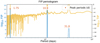 |
Fig. 1 FIP periodogram of a simulated system with three injected planets. The periods of the peaks are indicated by red points; the −log10FIP and log10TIP are represented as a function of the centre of the period interval considered, in blue and yellow, respectively. |
3.2.5 Relation with existing works
It is apparent in Eq. (8) that the TIP is a particular case of Bayesian model averaging (e.g. Hoeting et al. 1999) since we estimate the probability of a quantity of interest weighted by the posterior distribution of the alternative models defined. Barbieri & Berger (2004) introduce a quantity similar to the TIP, the posterior inclusion probability (PIP). This is defined in the context of linear regression where the data y (vector of size N) has a model y = Xβ + ϵ, X being a N × p, p < N, ϵ is a random noise and β a vector of p parameters. The alternative models are defined, corresponding to subsets of {1…p}. The PIP of index i, 1 =⩽ i ⩽ N is defined as the sum of posterior probabilities of models that include indices i. Barbieri & Berger (2004) show that the median posterior model (MPM), which is the model corresponding to indices with PIP > 0.5, under certain conditions generalised in Barbieri et al. (2021), has the optimal prediction error (quadratic penalty). The threshold of 0.5 simply means that it is more likely than not that i is non-zero. The TIP can be seen here as the prolongation of the PIP to the continuous parameter case.
The period selection of the FIP periodogram is made by marginalising over parameters other than period, as are the Keplerian periodogram (Gregory 2007a,b) and the AGATHA periodogram (Feng et al. 2017). Here we marginalise, in addition, over the number of planetary signals. Therefore, the FIP provides a single detection metric, which, furthermore, can be directly interpreted as a probability. The definition of the FIP periodogram in Sect. 3.2.4 is especially close, though not equivalent, to the quantity defined in Eq. (9) of Brewer & Donovan (2015), which is the sum of the posterior densities of the log periods of the planets in the model. The probability that there is at least one planet in a certain period interval l is equal to the sum on i of the probability of events ei: “the period of planet i is in I” provided the ei are disjoint, that is the probability of having two different planets in i is zero. In practice this probability is very small, but not strictly zero. If the quantity defined in Eq. (9) of Brewer & Donovan (2015) was binned, then this would be close to a FIP periodogram with a bin of constant size in log-period. Finally, Brewer & Donovan (2015) suggest using the posterior probability of the event Q := “a planet exists with period between 35 and 37 d”, which is also what we compute. In the following sections we examine the properties of using systematically the probability of such events (the TIP) as a detection criterion. In particular, in the next section we highlight a property of the FIP which can be seen as a Bayesian false discovery rate (Benjamini & Hochberg 1995).
3.3 Properties
3.3.1 Fundamental property
Property. One of the advantages of the quantity (7) is that it is easy to interpret. If the likelihood and prior accurately represent the data, and a series of statistically independent detections are made with FIP = α (or TIP = 1 − α), then, on average, a fraction 1 − α are true detections. More precisely, the number of true detections among M detections follows a binomial distribution B(M, 1 − α).
In practice, this has the following meaning. Let us consider a collection of intervals Ij and of RV datasets yj j = 1…n, such that the event “there exists a planet with period in Ij knowing data yj” are statistically independent, and such that  for a certain α between 0 and 1. The yj could be the same dataset or different ones, we only require independence of the events. Then, provided the likelihood and priors used in the computations of
  are correct,
 (9)
(9)
We can be even more precise: the number of times a planet with period P ∈ Ij and FIP = α was indeed present among M statistically independent detections follows a binomial distribution B(M, 1 − α).
Consistency test. The property (9) holds if the priors and likelihoods are exactly the same as those that generated the data, which is unlikely to happen in real cases. We suggest using Eq. (9) as a device to calibrate the scale of probability used to detect exoplanets. In principle, let us suppose that several datasets (for instance the HARPS data) have been analysed and FIPs are computed at time t1. As more data comes along, at t2 > t1 the presence of certain planets will be confirmed with very high probability. It is possible to check that statistically independent detections made at t1 with FIP α, are such that a fraction α of them are spurious, up to the uncertainties of a binomial distribution.
However, if property (9) is a necessary condition for RV models to be validated, it is not sufficient. The fact that it is satisfied does not guarantee that the RV models are all correct. The property (9) we put forward pertains to a frequency of events, while in Bayesian analyses probabilities are usually interpreted as subjective measures of belief, but as we discuss below this does not constitute a contradiction. The consistency test we suggest is a particular case of Bayesian model calibration (Draper & Krnjajic 2010).
Discussion. It has been mathematically established that in any system of quantitative measure of belief satisfying intuitive properties, the update of the belief measure in view of new information has to be made according to Bayes formula (Cox 1946, 1961, although see comments by Paris 1994; Halpern 1999). Probabilites are typically used as subjective measures in the Bayesian context. However, Cox’s theorem result does not give prescriptions on how to select the initial belief. In the case of exoplanet detection it seems to us that, among subjective measures, it is natural to desire that (1) a probability gives the actual fraction of times you would be wrong when claiming a detection with a certain significance and (2) the prior probability represents the distribution of elements in nature, as in a hierarchical Bayes model such as Hogg et al. (2010). If so, then Eq. (9) has to be satisfied. To illustrate our approach, we can consider the context of information theory (Shannon 1948), in which priors reflect the occurrence of a word in a certain context within a given language and the posterior probability of a word at the receiving end the communication channel reflects a frequency of errors. In the context of exoplanets, “words” would be the vector of orbital and stellar parameters of a system, and we would like them to be distributed according to the true distribution of planetary systems (the “language”). A given FIP threshold then corresponds to a concrete verifiable property, while a Bayes factor scale is harder to interpret. Tying the probabilities to frequencies within Bayesian analysis has been suggested in van Fraassen (1984); Shimony (1988) from an epistemological point of view.
One could argue that the influence of the priors vanishes as more data are acquired (Wald 1949), and, as a consequence, it is not necessary to tie the meaning of a prior to an observable, or operate the consistency test we suggest in this section. However, in the context of exoplanets the asymptotic regime (N → ∞) is not reached, and the influence of the prior is rarely negligible. Second, results showing the convergence of parameters estimate when N → ∞ regardless of the prior assume a certain form for the likelihood as a parametrised function, which might not accurately represent the noise properties. In the context of radial velocities, stellar noise models are unreliable, but if they were, Eq. (9) would be satisfied.
In conclusion, we believe that property (9) offers an intuitive interpretation of the FIP. Furthermore, it can serve as a model calibration test (Draper & Krnjajic 2010), although it will not give precise indications on whether the prior or the likelihood is faulty.
3.3.2 Aliasing
Radial velocities have a sampling that is irregular but close to an equispaced sampling with a step of one sidereal day (0.997 day) with missing samples. As such, periodogram signals at frequency ν0 typically exhibit aliases at ν0 + νs and −ν0 + νs, where νs = 1/0.997 day−1. As a consequence, it is uncertain whether the signal is at ν0 or ±ν0 + νs is the true signal (Dawson & Fabrycky 2010; Robertson 2018). The yearly and monthly repetition of the sampling patterns, and other gaps in the data potentially create more aliasing problems. The FIP periodogram provides insight into this problem; if there is a degeneracy between two periods the samples will be split between the two in proportion of the probability that they are supported by the data and assumed likelihood and priors.
Aliasing can also create problems when several signals are present, and might result in a high periodogram peak which does not correspond to any of the true periods (Hara et al. 2017). FIP periodograms also address that situation as, by design, several planets are searched at the same time.
3.3.3 Another perspective on error bars
The error bars on the orbital elements of a planetary system often are computed with MCMC methods (e.g. Ford 2005, 2006). Once the planets have been detected, the posterior distribution of the orbital elements are computed. The FIP can be generalised to express the probability that the model includes a planet with its orbital elements in a certain set. We can define the probability that there is a planet with orbital elements in a set S as
 (10)
(10)
Just as in the case of credible regions, we can define a sequence of probabilities (pi)i and a corresponding sequence of sets Si such that  . In this case we obtain regions of probability (pi)i, for which the uncertainties on the number of planets is propagated. This can be useful in particular for population studies. Instead of excluding planets that do not meet a certain detection threshold, we can take into account marginal detections with a rigorous account on the uncertainty on whether there is a planet.
3.3.4 Excluding planets
One of the properties of the formalism we develop is that it can put an easily interpretable condition on the absence of planets. The FIP, by definition, is the probability not to have a planet in a certain range. Excluding the presence of planets with a certain confidence might be of interest to study the architecture of planetary systems. For instance, it can be helpful to put constraints on the total mass of the planets and compare it to the minimum mass solar nebula (Hayashi 1981).
4 FIP: Practical computations
4.1 POLYCHORD
The computation method suggested in Sect. 3.2.2 requires computing the evidence Pr{y|k} of a model with k planets and the posterior of the orbital elements knowing the number of planets, p(θ|y, k). These two quantities can be computed with a nested sampling algorithm. In the present work we use POLY-CHORD (Handley et al. 2015b,a). By default we set the number of live points as 40 times the number of free parameters in the model.
4.2 Marginalising over linear parameters
As described in Sect. 2.1, our model of the data y is y = ƒ(θ) + ϵ, where ϵ is a random variable whose distribution is parametrised by β, and ƒ is a deterministic function. We now separate the model parameters θ into two categories: the model depends linearly on parameters x and non-linearly on parameters η. In Appendix C we show that provided the likelihood is Gaussian and the prior on the linear parameters x is a Gaussian mixture model, that the integral
 (11)
(11)
has an analytical expression.
Marginalising over linear parameters presents the advantage of reducing the number of dimensions to explore with the nested sampling algorithm. To reduce as much as possible the number of non-linear parameters, we rewrite the radial velocity due to a planet. Denoting it by υ(t), instead of
 (12)
(12)
where K is the semi-amplitude, t is the time, ν the true anomaly, e the eccentricity, and ω the argument of periastron, we write
 (13)
(13)
We obviously only use one offset C in our model, even if several planets are present.
The Gaussian mixture components would typically be chosen to represent populations such as super-Earths, mini-Neptunes (Fulton et al. 2017), Neptunes, and Jupiters. When the linear parameters are analytically marginalised, η and β are the only free parameters, such that only three parameters are used per planet instead of five: period, eccentricity e, and time of passage at periastron tp (or equivalently the initial mean anomaly). This idea is similar to the use of a Laplace approximation of the evidence marginalised on certain parameters (Price-Whelan et al. 2017).
When the prior on A and B in Eq. (13) is Gaussian with null mean and variance σ2, this translates to a Rayleigh prior on  with parameter σ. For simplicity, we refer to this situation as a Rayleigh prior on K with parameter σ, even though
  for e > 0.
4.3 Validation of the FIP computations
To validate our algorithms, we perform several tests on simulated data. Here, our goal is not to evaluate the performance of the FIP as a detection criterion, but to ensure that our numerical methods are retrieving a good approximation of Eq. (6). Claiming a detection is then: “there is a planet with period in interval I”. We see in Sect. 3.3.1 that when the prior and likelihood are correct, on average, a fraction α of independent detections made with a FIP α are spurious (see Eq. (9)), and a fraction 1-α is correct. If our numerical method is converging, then this property must be verified in practice.
We verified whether the property (9) is true on 1000 generated datasets. In the first test, we considered only circular orbits. The model of the signal is
 (14)
(14)
where ϵj is the noise. We consider ti from the first 80 measurements of HD 69830 (Lovis et al. 2006) (see dataset in Appendix B). The values of θ := k, (Ai)i=1…k, (Bi)i=1…k, C, and P are generated according to distributions shown in Table 1. We denote by G(µ, σ2) a Gaussian distribution of mean µ and variance σ2. Once a value of θ has been drawn, we create a dataset by drawing the ϵj from a Gaussian distribution of null mean and standard deviation given by the nominal uncertainties on the first 80 measurements of HD 69830 (typically 0.45 m s−1).
We now have 1000 datasets. For each of the RVs, we compute the FIP periodogram as defined in Sect. 3.2.4 with exactly the same priors and noise model as those used to generate the data. If our calculations of the FIP periodograms have converged, on average a fraction 1 − α of independent detections made with FIP = α should be correct.
We consider a grid of probabilities from 0 to 1, (αj)j=1…M. For each of the probabilities in the grid, we search for detections with FIP = αj. For instance, we fix α = 10% and search for intervals I such that the event “there is a planet with P ∈ I” has a FIP of 10%. If several events where the “presence of a signal in a certain period interval” have a probability αj for the same dataset, we select one of them randomly. As a result of this process, for each αj, for each generated system indexed by n, we selected at most one interval  such that the event “there is a planet in the interval
  ” has probability αj. If for system n there is no such event, we simply do not include system n in the computation.
Since for a given αj, the events “there is a planet in the interval  with FIP αj” we selected are independent, we expect from Sect. 3.3.1 that for a fraction αj of them, there is actually no planet in the interval. Equivalently, in a fraction pj = 1 − αj of them, there will actually be a planet.
More precisely, for fixed j, the events “there is a planet in the interval  ” should be independent realisations of a Bernouilli distribution of parameter pj. This means that the number of success (there is indeed a planet) divided by the number of events Nj should be on average pj with a standard deviation
  . In Fig. 2, upper panel, we represent the fraction of success as a function of pj as well as the error bar
  . We recall that for a given dataset n, when there are several events “there is a planet whose period is in the interval
  with probability αj”, we choose one event randomly. Points of different colour correspond to different realisations of the random choice. In the lower panel we represent the difference of the fraction of success and the TIP pj, divided by the error bar σj. In the upper panel, we expect a curve compatible with y = x, which seems to be the case. According to our hypothesis, the quantity plotted in the lower panel should be distributed with mean 0 and variance 1, which appears to be the case.
The same test was repeated in several configurations (e.g. zero to four planets, red noise, eccentric planets; see in Appendix D). In all cases we find an agreement between the expected and observed distribution of FIPs, with at most 2σ. We find the highest discrepancy in the simulation allowing highly eccentric orbits. We attribute this to the difficulty of exploring the parameter space of highly eccentric orbits, which contains a consequent amount of local minima, as shown in Baluev (2015) and Hara et al. (2019).
Priors used to generate and analyse the 1000 systems with circular orbits.
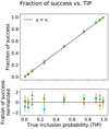 |
Fig. 2 Fraction of events with probability pj where there actually was a planet injected as a function of pj. The colours blue, orange and green correspond to different, random choices of events with TIP pj. |
5 Example: The FIP periodogram of HD 10180
In this section we compute the FIP periodogram of the HARPS data of HD 10180. This system is known to host at least six planets with periods 5.759, 16.35, 49.7, 122, 604, and 2205 days and minimum masses ranging from 11 to 65 M⊕ (Lovis et al. 2011). A re-analysis by Feroz et al. (2011) also supports the detection of six planets. Three other unconfirmed planets have been claimed in Tuomi (2012) at 1.17, 9.65, and 67 days. The first 190 points of the HARPS HD 10180 dataset have been analysed in Faria (2018, p. 66) with a trans-dimensional nested sampling algorithm (Brewer 2014), in which the number of planets freely varies with the other parameters. In the analysis of Faria (2018) it is found that, when taking as a detection criterion the Bayes factor and a detection threshold at 150, only six planets are found. However, it appears that taking a uniform prior on the number of planets, the peak of the posterior number of planets increases monotonically until 19 planets.
As in Faria (2018), we analysed the first 190 points of the HARPS dataset1. The radial velocity measurements span 3.8 yr (from BJD 2452948 to 2455376) and have a typical nominal uncertainty of 0.6m s−1. The data are presented in Appendix B. We used POLYCHORD (Handley et al. 20l5b,a) to compute the posterior distribution of orbital elements and the Bayesian evidence for models with a fixed number of planets. The FIP was then computed as described in Sect. 3.2.2, and the FIP periodogram defined as −log10 FIP(ω), where FIP(ω) is the FIP of the event “there is at least one planet with frequency in the interval [ω − Δω, ω − Δω]” with Δω = 2π/Tobs, Tobs being the observation time span (see Sect. 3.2 for details).
We computed the FIP periodograms with priors and likelihood summarised in Table 2. The prior on semi-amplitude is log-uniform, so that the analytical marginalisation of linear parameters described in Sect. 4.2 cannot be performed. We set the number of live points to 40 times the number of free parameters, that is 1360 live points for the six-planet model. Calculations are made on the DACE cluster (Univ. Geneva) of the LESTA server using 32 cores of the Intel(R)Xeon(R) Gold 5218 CPU @ 2.30 GHz.
A first calculation of the FIP of up to five planets shows that planets at 5.759, 16.35,49.7, 122, and 2205 days have a very low FIP (10−12), and are therefore detected with a very high confidence. To improve the convergence of the algorithm, we imposed restrictive priors on the periods of the five confidently detected planets. These are centred on the maximum likelihood estimate of these periods and have a width in frequency +2π/Tobs where Γobs is the total observation time span. This hypothesis changes the marginal likelihood, and in turn the PNP and the FIP. To correct for this, we adopted a new prior on the number of planets. Denoting by p(k) the prior on the number of planets k and p′(k) the new one, denoting by pB the broad prior on period chosen in Table 2, by pN the new narrow prior, and by P1,…P5 the periods of the planets confidently detected,
 (15)
(15)
The results are reliable only if our algorithm has converged. We performed the two convergence tests described in Sect. 3.2. We compared the FIP periodograms obtained with k and k + 1 planets. Figure 3 shows the FIP periodograms obtained with a maximum of six and seven planets (blue and purple, respectively). It appears that the FIP periodogram is essentially unchanged, so that we do not search for an additional planet. For a given number of planets, we performed several runs of POLYCHORD (here three) and ensured that the maximum difference of FIP periodogram over all frequencies is below a certain threshold. In Fig. 4, we represent three calculations of the seven-planet FIP periodogram obtained with different runs in green, blue, and purple. The maximum difference occurs at 600 days, and is below one. In Table 3 we summarise the results of our calculation. We provide the log evidence, its standard deviation across runs, the posterior number of planets and median runtime. It appears that, as in Faria (2018), the PNP is higher for the seven-planet model; however, the six-planet model is favoured by the FIP.
In Sect. 4.2, we state that when defining the prior on linear parameters as a Gaussian mixture model, calculations can be sped up. We perform the same calculations as above, but the priors defined on the linear parameters of Keplerian is a Gaussian mixture with two components of mean 0 and standard deviation 1 and 4 ms−1. We note that if we wanted to define super-Earths, mini-Neptunes, and Neptune populations more closely and match a mass distribution, we would need to make the standard deviation of the two components of the Gaussian mixture model depend on the period of the planets, as in Ford & Gregory (2007), which is not done here for the sake of simplicity. We use a number of live points equal to 50 times the number of free parameters. Since we use the analytical marginalisation over linear parameters presented in Sect. 4.2, there are only three parameters per planet instead of five. For the six-planet model, there are 1100 live points. Figure 5 shows the FIP periodograms obtained with a maximum of six and seven planets (blue and purple, respectively). In Fig. 6, we represent three calculations of the seven-planet FIP periodogram obtained with different runs in green, blue, and purple. In this case the difference across runs is more important and the significance of the 600-day signal is much higher. This last point illustrates that the prior on semi-amplitude can have a non-negligible effect on the significance of signals. In this case the run-to-run difference is more important as well as the six- versus seven-planet test. It appears that in the seven-planet models there is a degeneracy between the 2400-day planet and longer periods. However, as shown in Table 4, the runtime for six and seven planets is 4 h 46 min and 14 h 59 min as opposed to 9 h 42 min and 34 h 14 min for the log-uniform prior.
For both prior choices, it appears that even though the Bayes factor and PNP slightly favour a seven-planet model, the FIP provides the detection of six planets. We also found that the choice of the semi-amplitude prior has an important effect on the significance of small amplitude signals. This aspect is discussed in Sect. 6.3.
Priors used for the computation of the FIP periodogram of HD 69830.
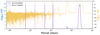 |
Fig. 3 FIP periodogram of 190 HARPS measurements of HD 10180 computed with a log-uniform prior on semi-amplitude on [0.1, 20] m s−1. In blue: FIP periodogram for up to six planets; in pink: FIP periodogram for up to seven planets. |
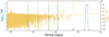 |
Fig. 4 FIP periodogram of 190 HARPS measurements of HD 10180 computed with a log-uniform prior on semi-amplitude on [0.1,20] m s−1. In blue, pink, and green: FIP periodograms corresponding to different runs of calculations of posterior distributions of the parameters of a seven-planet model. |
Parameters of the different runs of POLYCHORD on the HD 10180 dataset, when using a log-uniform prior on semi-amplitude.
6 Comparison of the metrics
6.1 Outline
In this section, we discuss the properties of the FIP and other detection criteria. First, in Sect. 6.2 we compare the performance when the model is known. We then study whether the detection criteria are sensitive to prior and likelihood choices in Sects. 6.3 and 6.4, respectively.
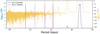 |
Fig. 5 FIP periodogram of 190 HARPS measurements of HD 10180 computed with a Gaussian mixture model linear parameters (two components with σ = 1 and 4ms). In blue: FIP periodogram for up to six planets; in pink: FIP periodogram for up to seven planets. |
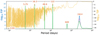 |
Fig. 6 FIP periodogram of 190 HARPS measurements of HD 10180 computed with Gaussian mixture model linear parameters (two components with σ = 1 and 4 ms). In blue, pink, and green: FIP periodograms corresponding to different runs of calculations of posterior distributions of the parameters of a seven-planet model. |
Parameters of the different runs of POLYCHORD on the HD 10180 dataset when using a Gaussian mixture prior on semi-amplitude.
6.2 Performance comparison of the different metrics when true model is known
6.2.1 Simulation
To compare the different methods we considered a set of 1000 simulated datasets, with zero to two injected circular planets. The planet signals are generated with a log-uniform distribution in periods from 1.5 to 100 days, uniform phase, and a Rayleigh distribution in amplitude with σ = 1.5m s−1. This allows us to use the analytical marginalisation on linear parameters described in Sect. 4.2, which speeds up computations. The distributions of elements are summarised in Table 1. The time stamps are taken from the first 80 HARPS measurements of HD 69830 (Lovis et al. 2006) (see dataset in Appendix B) and the noise is generated according to the nominal error bars, which are typically 0.54 ± 0.24 m s−1.
We then generated another set of 1000 systems with a lower S/N. The simulation is made with identical parameters except that a correlated Gaussian noise is added. This one has an exponential kernel with a 1 m s−1 amplitude and a timescale τ = 4 days. These simulations are intentionally simple, to enable the identification of the hypotheses driving the results.
6.2.2 Analysis
We analysed the data with different methods. In all cases, correct likelihood and priors are assumed. In particular, we searched for up to two planets, according to the input data. Except the PNP, we evaluated the methods with a grid of detection thresholds. For a given detection threshold, the methods proceed as follows:
Periodogram + FAP: We compute a general linear periodogram, as defined in Delisle et al. (2020), with the same grid of frequencies as used to generate the data (from 1.5 to 100 days) and the correct covariance matrix. If the FAP (as defined in Sect. 2.2) is below a certain threshold fixed in advance, we add a cosine and sine function at the period of the maximum peak to the linear base model and recompute the periodogram. The planet is added if the FAP is below the FAP threshold. We do not search for a third planet.
Periodogram + Bayes factor: Same as above, but here the criterion for adding a planet is that the Bayes factor (as defined Sect. 2.3) is above a certain threshold. The evidence (Eq. (3)) is computed with the distributions used in the simulations; in particular, the period is left free between 1.5 and 100 days;
ℓ1 periodogram2 + FAP: We compute the ℓ1 periodogram (Hara et al. 2017) with the same grid of frequencies as used to generate the data (from 1.5 to 100 days). If the FAP of the maximum peak is below a certain threshold, it is added to the base model of unpenalised vectors, the A periodogram is recomputed, and the FAP of the maximum peak is assessed. If it is below a certain threshold, the planet detection is claimed. We do not look for a third planet;
ℓ1 periodogram + Bayes factor: same as above, but here the criterion for adding a planet is that the Bayes factor (as defined in Sect. 2.3) is above a certain threshold;
FIP: we compute the FIP periodogram as defined in Sect. 3.2 and select the two highest peaks. We select a period if its corresponding FIP is below a certain threshold;
PNP + FIP periodogram: To select the number of planets we order the peaks of the FIP periodogram by increasing FIP. We select the number of peaks corresponding to the highest PNP, as defined in Sect. 2.4;
FIP periodogram + Bayes factor: the periods are selected as the highest peaks of the FIP periodogram and the number of planets is selected with the Bayes factor. This procedure is very close to Gregory (2007b,a) except that we use the FIP periodogram instead of the marginal distribution of periods for each planets. We do not take the approach of Gregory (2007b,a) to select the periods as nested sampling algorithms such as POLYCHORD tend to swap the periods of planets, such that marginal distributions are typically multi-modal;
FIP periodogram + FAP: The periods are selected as the highest peaks of the FIP periodogram and the number of planets is selected with the false alarm probability.
For the computation of Bayes factor, FIP, and PNP, the number of live points in the nested sampling algorithm is equal to 200 times the number of planets in the model.
6.2.3 Performance evaluation
To evaluate the performance of the different analysis methods, we use two criteria: the ability of the methods to retrieve the correct number of planets, and their ability to retrieve the planets with the correct periods. To assess the correct retrieval of the number of planets, we simply count how many planets are detected. We measure the difference between the number of planets claimed and the true one. If this difference is strictly positive or negative, we count them respectively as a false positive and a false negative. For instance, if there are two detections while no planet is present, we count two false positives. The total number of mistakes is given by the sum of false negatives and false positives on the 1000 systems analysed.
To verify that periods are appropriately retrieved, we check whether a frequency found is less than 1/Tobs away from the true frequency, Tobs being the observation time span. For a given detection threshold and a given simulated system, we consider the planets detected with decreasing significance. If a planet is claimed, but does not correspond to a true planet with the desired precision on period, or if no planet is present, it is labelled as a false detection. If the claimed planet corresponds to a true planet, we label it as a correct inference and remove its period from the set of true periods, so that a planet cannot be detected twice. The situation where no planet is claimed but there is a planet in the data, is labelled as a missed detection. The total number of mistakes is the sum of missed and false detections on the 1000 systems.
The rationale of evaluating the different methods presented in Sect. 6.2.2 is to determine whether the performance of a given method comes from the period selection or the scale of the significant metrics. Periods are typically refined by a MCMC algorithm, but this changes the estimate of the frequency by a small fraction of 1/Tobs.
6.2.4 Simulation 1: White noise
In the first simulation, we only have white noise with a typical ratio of semi-amplitude to noise standard deviation of 3.4. The number of mistakes for the different detection metrics are shown in Fig. 7. The figure shows the performance in terms of retrieval of the number of planets (left column) and retrieval of the number and periods of the planets (right column). Each row corresponds to a different detection metric. The total number of false positives, false negatives, false detections, and missed detections on the 1000 systems are represented, as well as the minimum number of mistakes and the minimum and maximum thresholds at which this minimum is attained. In all cases, the x axis is oriented such that from left to right the detection criterion is more and more stringent (confidence increases). As might be expected, for each performance metric we find a U-shaped curve. When the detection criterion is permissive, the total error is dominated by false positives or false detections. Conversely, as the detection criterion becomes more stringent, detections due to random fluctuation are progressively ruled out and the detection errors are dominated by false negatives or missed detections. We note that the thresholds for which a low false positive rate is expected would typically be chosen, and it is in this range of thresholds that the methods should be compared.
We find that in terms of number of planets (left column in Fig. 7), all the significance metrics exhibit similar behaviour, with a minimum number of errors of 34–46. For comparison, a uniform random guess of the number of planets (0, 1, or 2) would yield a total of 888 errors on average. We find that the maximum PNP leads to the smallest error, as well as a iog Bayes factor close to 0 (see the plain grey line in third plot from the top). This is to be expected, since the maximum PNP has opti-mality properties, and the Bayes factor is designed to compare the number of planets by averaging over all the possible values of the parameters for a given number of planets. In all cases we see a sharp decrease in the number of false positives as the detection threshold becomes more stringent.
Larger discrepancies in performance happen when the methods are evaluated on their ability to retrieve not only the correct number of planets, but also the correct periods. In this case the periodogram + FAP and BF (two upper plots) exhibit similar performance. The A periodogram and FIP (three lower plots) exhibit better performance finding the periods of the planets in two ways: the minimum number of mistakes is smaller and the ratio of false positive to false negative is smaller at the optimum value.
The scales of thresholds (BF, FAP, FIP) are not in the same units. To further compare the methods, we compute the total number of mistakes in terms of correct retrieval of period and number of planets as a function of the number of false detections. This is plotted in Fig. 8, where we see that in the regime of low number of false positives (stringent detection criterion), there are important differences between the methods. For instance, for ten false positives (red dashed line) the methods exhibit very different performances. We checked that these results are not too dependent on the success criterion by labelling a detection false if the frequency found departs by more than 2/Tobs and 3/T0bs from a true period, instead of l/Tobs. The results are qualitatively identical. In conclusion, the FIP provides a low number of missed detection even when the number of false detections is small.
The performance of the ℓ1 periodogram and the FIP comes from the fact that both methods encode the search for several planets simultaneously. On the other hand, since the periodogram searches for one planet at a time, there are cases where the maximum of the periodogram does not occur on any of the true periods (see Hara et al. 2017). A detailed analysis shows that at stringent detection criteria for the Periodogram + FAP and Periodogram + BF, almost all of the false detections made by the methods occur in cases where there are two planets present in the data, and the period selection method selects a spurious peak. The FIP, FIP periodogram + BF, and FIP periodogram + FAP methods, where periods are selected from the FIP periodogram, exhibit much better performance. The performance is similar; a difference is seen only in the region with a low number of false positives (<12) (lower left, Fig. 8) where the FIP leads to a slightly lower number of false negatives. This suggests that not only is the period selection more efficient with a FIP periodogram, but that the significance scale on which the FIP is defined performs well in distinguishing true planets from false detections.
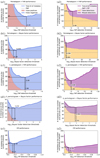 |
Fig. 7 Total number of mistakes on the number of planets (left) and number and period of planets (right) out of 1000 datasets with white noise (simulation 1, see Sect. 6.2.4) as a function of the detection threshold for different statistical significance metrics. From top to bottom: Periodogram + FAP, Periodogram + Bayes factor, ℓ1 periodogram + FAP, and FIP. The total number of false positives and false negatives are represented as light red and blue shaded areas. The false and missed detections are represented in orange and purple shaded areas, respectively. The minimum and maximum values of the detection threshold corresponding to the minimum number of mistakes are indicated with black lines. |
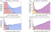 |
Fig. 7 continued. Same quantities as above, for the detection criteria FIP periodogram + FAP (f1 and f2) and FIP periodogram + Bayes factor (g1 and g2). |
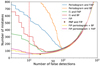 |
Fig. 8 Number of mistakes as a function of the number of false detections (log scale) for the different detection methods. The number of mistakes is defined as the sum of missed true planets and false detections. The data corresponds to simulation 1 (see Sect. 6.2.4): a random number of planets equal to 0, 1, or 2; the noise is white and Gaussian with semi-amplitude to noise ratio of 3.5. |
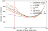 |
Fig. 9 Number of mistakes as a function of the number of false detections (log scale) for the different detection methods. The data corresponds to simulation 2 (see Sect. 6.2.5): a random number of planets equal to 0, 1, or 2 planets per system; white and correlated noise. This simulation has a timescale of 4 days and an amplitude of 1 m s−1. The semi-amplitude to noise level ratio of 1.7. Mistakes are defined as the sum of missed and false detections. |
6.2.5 Simulation 2: Lower S/N
In this simulation the exact same parameters as in simulation 1 are used to generate the data, except that we add a 1m s−1 correlated noise with a four-day exponential decay and a timescale. In this case the typical semi-amplitude to noise ratio is 1.65, as opposed to 3.48 in the previous simulation. The results are represented in Fig. 10 with the same conventions as Fig. 7. We add the red dashed lines to indicate the detection threshold at which there are only ten false positive claims. In Fig. 9, we represent the total number of mistakes as a function of the number of false detections (which therefore includes whether the period of planets is appropriately recovered).
Both in terms of optimal thresholds and mistakes at low false positive rates, the differences in performance between different analysis methods are less important. We attribute this to the fact that the noise level is higher, such that all signals are on average less significant, including spurious peaks. We observe that the FIP still outperforms the other methods. Here too, we see a difference in performance in the region with a low number of false detections (<12), where the FIP leads to a lower number of missed detections.
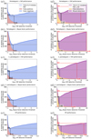 |
Fig. 10 Total number of mistakes on the number of planets (left) and number and period of planets (right) out of 1000 datasets with correlated noise (simulation 2, see Sect. 6.2.5) as a function of the detection threshold for different statistical significance metrics. From top to bottom: Periodogram + FAP, Periodogram + Bayes factor, ℓ1 periodogram + FAP and FIP. The total number of false positives and false negatives are represented in light red and blue shaded areas. The false and missed detections are represented in orange and purple shaded areas, respectively. The minimum and maximum values of the detection threshold corresponding to the minimum number of mistakes are marked with black lines. |
6.2.6 Summary
Threshold selection. In the previous sections, we have studied the number of false and true detections as a function of the detection threshold. In practice, a FIP level below which a detection is claimed would be set in advance. In this paragraph, we discuss the choice of this level.
The number of false positives for a given FIP threshold is linked to the intrinsic distribution of signals. To show this, let us consider two limiting cases, one where signals are extremely clear, and the other where they are very close to the noise level. In the first case there is a clear-cut separation between signals which are confidently detected and non-detections. A high FIP threshold, even 90%, might already provide a very low, potentially null number of false positives, since signals with FIPs less than 90% would typically have a very low average FIP. If the signal amplitudes are closer to the noise, then the FIPs of the maximum peaks will be concentrated towards higher values. This is observed in practice. The signals of simulation 2 have a lower average signal-to-noise ratio than those of simulation 1. For a FIP threshold at 10%, the expected number of false detections is the sum of the FIPs of all the signals of the simulation with FIP less than 10%. In simulations 1 and 2, this sum is 1.5 and 4.7, which is close to the number of observed false positives when using a 10% FIP detection threshold, two and six, respectively.
A 10% FIP threshold seems very permissive, and it might be surprising to observe only two and six false detections at this level for simulations 1 and 2, respectively. To have a more interpretable threshold, the sum of FIPs of signals can be used. For instance, in RV surveys, instead of using a fixed FIP detection threshold for each candidate signal, the signals found in the survey can be ranked with increasing FIP, and the detected signals are those with the lowest FIP such that the sum of the FIPs is less than a number n. It means that less than n false detections are expected over the whole survey. This approach is similar to the false discovery rate, used in a frequentist framework (Benjamini & Hochberg 1995).
It appears in Sects. 6.2.4 and 6.2.5 that the optimal FIP threshold in the simulations is 10−0.13 = 0.74. The optimal FIP threshold should be of the order of 50%. If the FIP is below 50%, it is more likely that there is a planet than not. In both simulations a FIP threshold of 1 to 10% appears to be appropriate. In real cases, the number of planets is unknown and model errors might create spurious signals. We therefore consider 1% to be an appropriate threshold.
Performance. In the two simulations, both the period selection and the level of significance play a role in the performance of the method. In Figs. 8 and 9, the methods using the periodogram, ℓ1 periodogram, and FIP periodogram perform increasingly better. The strong influence of the period selection method here comes from the relatively small number of observations, which results in aliasing.
We find that for the periodogram and ℓ1 periodogram the FAP performs better as a detection threshold than the Bayes factor, but this is the reverse for the FIP periodogram. Overall, the FIP as a detection criterion offers the best performance in the low false positive regime. It can in fact be shown to be optimal: it minimizes the expected number of missed detection for a certain tolerance to false ones (Hara et al. 2022a).
These results are obtained for priors corresponding to the distributions with which the data was generated. In the following sections, we consider the influence of the prior and likelihood choices.
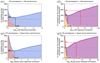 |
Fig. 10 continued. Same quantities as above, for the detection criteria FIP periodogram + FAP (f1 and f2) and FIP periodogram + Bayes factor (g1 and g2). |
6.3 Sensitivity to the prior
All planet detection criteria depend on the underlying distribution of planets (e.g. the true distribution in nature of semi-major axes, mass eccentricities). In the cases of the BF, PNP, and FIP the prior distribution has to be explicitly defined, and it may or may not represent accurately the true population. The definition of the FAP does not involve a prior, but the detection performance of the FAP also depends on the true population, in particular on whether the event sought after is rare or common (e.g. Soric 1989). In this section we focus on the effect of the prior choice on the detection properties of the criteria that explicitly use a prior distribution. To do so, we perform a simulation. We generate 1000 datasets with priors from Table 1 and a beta distribution on eccentricity with α = 0 and b = 15. As in the previous sections, in this simulation the semi-amplitude has a Rayleigh distribution with σ = 1.5 m s−1 (see Sect. 4.2), and the period has a log-uniform distribution on 1.5–100 days. We then analyse the data assuming the following:
Correct priors;
Correct priors except on periods, where it is assumed log-uniform on [1.5, 10000] days. In this case the periodograms and ℓ1 periodograms are computed on the period range [1.5, 10000] days;
Correct priors except on semi-amplitude, where it is a Rayleigh distribution with σ = 3m s−1 (i.e. twice the true σ);
Correct priors except on semi-amplitude, where it is assumed log-uniform on [0.1, 10] days.
We focus the discussion on the effects of these wrong assumptions on the ability of the methods to retrieve both the correct number and period of planets. As described in Sect. 6.2.3, we consider that a planet is successfully recovered if it is significant and its frequency is retrieved to an accuracy <1/Tobs where Tobs is the observation time span.
In Fig. 11, we represent the number of false detections (dashed lines) and total number of mistakes (plain lines) on the 1000 systems analysed as a function of the threshold adopted. These plots are identical to those in Figs. 7 and 10 except that we overplot the results obtained with different priors. Each plot corresponds to a detection method (from top to bottom: Periodogram + BF, ℓ1 periodogram + BF and FIP as described in Sect. 6.2.2). The colours blue, purple, yellow, and red correspond to assumptions on the prior listed above 1, 2, 3, and 4 respectively. We note that for a given detection threshold the variation in the number of mistakes is at most 25% in the regions where the number of false positives is below 50 out of 1000 systems, which is the region of interest. We find that prior 2 (prior larger on period, purple curve) performs similarly to or more poorly than other priors. This is explained by the fact that a larger prior on period offers chances to select a planet with period in the 100–10 000-day region, which would automatically be a false positive since planets are generated between 1.5 and 100 days. On the other hand, having a larger prior penalises the addition of a planet, such that viable candidates are not deemed significant with the larger prior. Finally, we note that for the FIP, prior 4 exhibits the worst performance: the number of false positives (red dashed line) decreases much more slowly than for the other priors. The method FIP periodogram + Bayes factor exhibits a pattern similar to the FIP. To further compare these methods, we plot in Fig. 12 the total number of mistakes as a function of the number of false detections, as in Figs. 8 and 9. The different colours correspond to different priors with the same conventions as in Fig. 11, plain lines correspond to the FIP and dashed lines to FIP periodogram + Bayes factor. In both cases the performance degrades most for the log-uniform prior on K, and gets closer to the ℓ1 periodogram + FAP (grey dotted line).
These observations are explained by the fact that changing the prior might change the level of significance (the Bayes factor) as well as the posterior distribution of periods and semi-amplitude, and in turn the period selected for the planets. On the change in Bayes factor, we found in our simulations that changing the prior from case 1 (the correct one) to 2, 3, or 4 only induces a multiplicative factor on the Bayes factor. Denoting as BF; the Bayes factors obtained with prior i, we perform a linear regression, log10 BFi = ai log10 BF1 + bi. The values of BF2 as a function of BFı are represented in Fig. 13 (blue and orange points correspond respectively to Bayes factors of 1 vs. 0 and 2 vs. 1 planets) the linear model is shown in black. We find a2 = 1.00, b2 = 0.48, and a root mean square (RMS) of the residuals RMS2 = 2.83. This means that when using prior 2 while the data was generated with prior 1, the Bayes factor is overestimated on average by a factor ≈100.48 = 3 with typical variations of a factor 102 83 = 676 around this value. For i = 3, we find α3 = 100, b3 = −0.55, RMS3 = 1.16, such that the dispersion around the linear model is smaller. For i = 4, α4 = 1.00, b4 =0.41, RMS4 =2.31. In Appendix E we study analytically the effect of priors on semi-amplitude as they get wider. We show that once the prior encompasses the high likelihood region, as it widens it penalises models with more planets. In terms of detection threshold, for instance in case 3, it means that having a Gaussian prior of 1.5 m s−1 and a detection threshold at BF = 100 is very similar to having a Gaussian prior of 3 m s−1 and a detection threshold of BF = 100/3.5 = 28, provided the candidate periods of the planets are identical in both cases.
However, changing the priors might change the posterior distribution of periods and semi-amplitudes, the convergence of numerical methods and in turn the peaks selected by the FIP periodogram. This indeed happens when using log-uniform semi-amplitude (prior 4 in the list above) instead of 1, 2, or 3. We investigate closely the ten false positives with the lowest FIP when using prior 4. It appears that all of them happen in the same situation: there are two planets truly in the data, and the incorrectly selected period appears at one of the two principal aliases of a true planet. Denoting by ω0 the frequency of the true planet, the spectral window is such that we expect aliases at ±ω0 + Δωi where i = lor 2, Δω1 = 1/0.997 days−1, and Δω2 = 1/31 days−1.
Our interpretation is that this is due to the different behaviours of Rayleigh and log-uniform priors close to small amplitudes, as well as potential remaining numerical errors. The results for the log-uniform on semi-amplitude (prior 4, red curves in Fig. 11) are obtained with ten times as many live points as other simulations (increasing the number of live points leaves the behaviour of the other metrics unchanged). With the original number of live points the number of mistakes in the low false detection rate regime was higher. The algorithm might spuriously select aliases. Second, the behaviour of the prior close to small amplitudes plays a role. In Fig. 14, we represent the priors on Κ considered here (in blue, yellow, and red solid lines the priors of assumptions 1, 3, and 4) and the ratios of priors (dotted lines). The orange dotted line represents the ratio of the log-uniform and Rayleigh prior with σ = 3 m s−1. It appears that the log-uniform prior is 195 times higher than the Rayleigh prior (σ = 3m s−1) at Κ = 0.1m s−1, and on average 20 times higher on the interval 0.1–1 m s−1, which artificially enhances the significance of low amplitude signals, given that they are very rare in our simulation. It appears that in the case of prior 4, the incorrectly selected aliases usually correspond to signal of smaller amplitudes (<0.5m s−1), which are boosted by the log-uniform prior with respect to the true amplitude of signals, which is >1 m s−1.
We finally note that changing the prior on the orbital elements should also be coupled to a change in the number of planets expected. If the prior on the period, semi-amplitude, or eccentricity is extended, then a higher yield of planets is expected. Let us consider the period case. The Titius-Bode law states that planets are typically uniformly spaced in log semi-major axis. If the search is initially performed with a log-uniform prior on a period between 1 day and P, then with a log-uniform prior on periods between 1 and twice as many planets will be expected. The increase in the expected number of planets compensates the penalisation introduced by having a wider period prior.
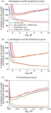 |
Fig. 11 Total number of mistakes (plain line) and total number of false detections (dashed lines) on 1000 simulated systems as a function of the threshold (from top to bottom: periodogram + BF, ℓ1 periodogram and BF, FIP) for different assumptions on the priors (see Sect. 6.3). In blue: correct priors (1.5–100 days log-uniform in period Rayleigh with σ = 1.5 ms−1 on K); in purple: 1.5–10 000 days log-uniform in period; in yellow: Rayleigh with σ = 3m s−1 on K; in red: log-uniform on [0.1, 10] m s−1 on K. The dashed lines represent the number of false detections as a function of the detection threshold and plain lines represent the total number of mistakes (false and missed detection) as a function of the threshold. |
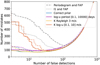 |
Fig. 12 Number of mistakes (false detection + missed detections) as a function of the number of false detections obtained with the FIP for different priors. The plain lines represent the detections with the FIP and dashed lines with FIP periodograms + Bayes factor. |
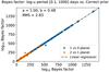 |
Fig. 13 Logarithm (base 10) of Bayes factor comparing models with 1 vs. 0 (blue) and 2 vs. 1 (orange) planets computed on 1000 simulated RV time series (black points). In abscissa the Bayes factor is computed with correct priors. In ordinate, the Bayes factor is computed with identical priors except on period, where the prior width is log-uniform on [1.5, 10 000] days instead of [1.5, 100], The red line represents a linear regression. |
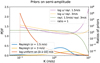 |
Fig. 14 Priors on semi-amplitude. The red, yellow, and blue curve correspond to Rayleigh priors with σ = 1.5, σ = 3m s−1, and log-uniform on [0.1 – 10]m s−1. The blue dotted line indicates the 0.1m s−1 limit. Shown is the ratio of log-uniform to Rayleigh priors (dashed lines), and of the 1.5 and 3 m s−1 Rayleigh priors (scale is on the right y-axis). |
6.4 Sensitivity to the likelihood: Averaging over noise models
Detections are sensitive to prior information, but also to the likelihood choice, which translates our assumptions on the noise. This is especially critical in the context of exoplanet detections, in which correlated stellar noise plays a crucial role. In this section, we study the sensitivity of detections as a function of the method used to estimate the noise parameters. As in Sect. 6.3, we perform a simulation. We generate 1000 datasets whose parameters follow the distributions listed in Table 1. On each dataset, we generate an additional correlated Gaussian noise with an exponential kernel, a decay timescale of 4 days and an amplitude of 1 m s−1, as in Sect. 6.2.5. Additionally, we generate a time series with exactly the same noise properties (the same covariance). This is meant to simulate an activity indicator which could have the same covariance properties as the radial velocities.
These datasets are analysed with the priors and likelihood that were used to generate the data, except on the noise. We analyse the data with the FIP with two different noise models. In the first one, we perform a maximum likelihood fit of the noise parameters (amplitude and timescale) onto the simulated activity indicator, and use the fitted values as fixed noise parameters in the analysis of the RV. In the second model, the noise timescale is allowed to vary with a uniform prior on 0–15 days and an the amplitude with a uniform prior on 0 to 4 m s−1.
The results of these simulations in terms of false and missed detections are represented in Fig. 15 (fitted noise) and Fig. 16 (free noise), we show the number of false (yellow) and missed (purple) detections as a function of the FIP threshold. When using a free noise model, the minimum number of mistakes is 418 compared to 510 in the fitted noise case.
To provide some intuition on the role of the noise parameters in detection capabilities, we consider the calculation of a periodogram with a fixed noise model. We compute the average value of the periodogram when the true covariance of the noise is Vt while the analysis is made with covariance Va, and divide it by the average value of the periodogram when the noise is generated and analysed with Vt. This quantity expresses to what extent the periodogram is over- or underestimated under incorrect assumptions on the noise. In Delisle et al. (2020), an analytical expression of this quantity is provided. To simplify the discussion, we assume that both true and assumed covariances consist of nominal error bars and a noise of covariance  . Let us denote the true timescale and amplitude of the noise by τt, σR,t and the assumed timescale and amplitude by τt, σR,a. We assume σR,a = σR,t and consider the expectancy of the ratio of periodograms obtained assuming τa and τt, supposing the signal contains only noise with timescale τt. In Fig. 17, we show this value computed with the time stamps used to generate the data, for τt = 4 days. If τa = τt, the expected ratio of periodograms is one, which is represented in black. We represent the periodogram ratio for τa = 1, 2.5, 6, and 8 days, represented in colours from blue to red. We see that if the timescale of the noise is underestimated (τa = 1 or 2.5 days), then we overestimate the power at low frequencies, resulting in too high a confidence in detections at these periods. Conversely, at lower periods (≈1–10 days), we underestimate the periodogram power. Because of aliasing, close to one day, the behaviour is closer to that of the low frequencies. This situation is reversed when the noise timescale is overestimated. In this case the power at low and high frequencies is respectively under- and overestimated.
This discussion provides some intuition as to why it is advantageous to average the detection metric over noise models, and why it is important to have alternate models that can encompass the true autocorrelation of the noise). The noise parameters, in particular timescales, are allowed to be greater or lower than the true noise timescale, such that the significance of a given period will be naturally balanced. On the contrary, if the noise is fitted and its timescale is under- or overestimated, this acts like a frequency filter that enhances or reduces the significance of signals depending on their periods.
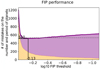 |
Fig. 15 Total number of false and missed detections (yellow and purple shaded areas, respectively) on 1000 systems as a function of the FIP threshold when selecting the noise model with a fit of the ancillary indicators. |
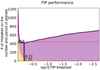 |
Fig. 16 Total number of false and missed detections (yellow and purple shaded areas, respectively) on 1000 systems as a function of the FIP threshold when the noise model is free to vary. |
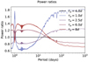 |
Fig. 17 Expectancy of the ratio of periodograms computed with a noise with exponential covariance τa and the true timescale τ = 4 days. Each curve corresponds to a different value of τa: 4 days (black) and 1, 2.5, 6, and 8 days (lavender to red). |
7 Conclusion
The goal of the present work was to determine good practices for the analysis of radial velocity data, given that assumptions on the priors and the noise model (the likelihood) might be incorrect. We noted that the existing significance metrics (Bayes factor; e.g. Gregory 2007b) and false alarm probability (FAP) (e.g. Scargle 1982; Baluev 2008) do not exactly define the information needed to claim a planet detection, which cannot be made without an estimate of the period of the planet. The computation of Bayes factor and FAP need to be coupled to an analysis of the period of the planets such as a periodogram (e.g. Baluev 2008), a ℓ1 periodogram (e.g. Hara et al. 2017), or the analysis of the marginal distribution of periods (e.g. Gregory 2007b). Furthermore, Bayes factors and FAP are defined on scales that are difficult to interpret.
To address this issue, we defined a new statistical significance metric, the true inclusion probability (TIP), which by definition is the probability to have a planet in a given period interval, and the false inclusion probability (FIP), defined as 1 − TIP (see Sect. 3.2.1). This criterion can be defined in a general setting of parametric signals detection, and be shown to optimally balance false and missed detection (Hara et al. 2022a). In particular, it can serve as a detection criterion for other exoplanet detection methods (transits, astrometry…) and any type of parametrised periodic variation in time series.
In the context of exoplanet detection with RV, we suggested computing the FIP on a sliding frequency interval of fixed length to produce a periodogram-like figure, which we call FIP periodograms, and to select the planets based on peaks with FIP values below a certain threshold (see Sect. 3.2). The FIP can be computed in two ways: with algorithms sampling orbital elements for a given number of planets (see Sect. 3.2.2) and trans-dimensional algorithms, able to sample directly the joint posterior of the number of planets and orbital elements (see Sect. 3.2.3). We defined two convergence tests: for a given maximum number of planets, we can run the calculation of FIP periodograms several times and ensure that the values are sufficiently close to each other in a user-defined sense. Second, to determine the maximum number of planets, we can stop once the difference of FIP periodograms obtained with an additional planet is below a threshold, here also user-defined (see Sect. 3.2.4). We have highlighted the following properties of the FIP:
The FIP has a clear meaning. If the model used in the analysis is correct, on average, a fraction 1 − α of statistically independent detections made with FIP = α are correct. This property can be applied to check that the signal models (likelihood and priors) are appropriate. The FIP gives a prediction on the number of true and false detections that can be checked on a given RV catalogue (see Sect. 3.3.1)
The FIP has a built-in period search, such that it offers clear diagnoses of aliasing. It mitigates the false detections linked to combination of aliases leading to detections at spurious periods (see Sect. 3.3.2);
The framework of the FIP allows us not only to detect, but also to exclude planets within a certain model, since by definition it is the probability of having no planet in a certain range (see Sect. 3.3.4).
In Sect. 6, we studied the performance of the FIP as well as those of existing significance metrics. We discussed the best practices in three cases: assuming the model used in the analysis is the same as the one with which the data was generated, in the case where the prior does not correspond to the distributions of the generated elements, and finally in the cases where the true noise model is unknown. Our findings are summarised below:
In our simulation the FIP offers the lowest number of false detections (planets detected at the wrong period, or when no planet is present) and missed detections (no planet detected when there is a planet). The difference with other methods is particularly important when the detection threshold corresponds to low false positives. In that regime the FIP still offers a low number of missed detections. As a comment, in high false positive regimes, all statistical metrics seem to have the same behaviour;
Detections are sensitive to the priors chosen on semi-amplitudes and periods. The behaviour of the prior close to low amplitudes is especially critical for the significance of low amplitude planets such as Earth-like planets. A further study of the priors to be chosen in this regime will be crucial;
It is better practice to let the noise parameters vary than fixing them to fitted values, for instance values fitted on ancillary spectroscopic indicators such as bisector span (Queloz et al. 2001) or log R′HK (Noyes 1984);
The optimal FIP threshold in terms of minimal number of false positive plus false negative is close to 50%. A threshold of 1% appears conservative and appropriate, but there is no need to define a clear-cut threshold. Alternatively, when analysing a RV survey, it is possible to set a detection threshold on the sum of the FIPs of the candidate signals, which is the expected number of false detections (see Sect. 6.2.6).
We note that all our simulations were intentionally simple, to isolate the effects of different assumptions. In the simulations, the maximum number of planets is known, and that the combinations of periods could be un-physical. Further comparisons on more realistic data such as in Pinamonti et al. (2017) would be valuable.
The framework of the FIP is concerned with explicit alternatives, for example 1, 2, or 3 planets and specified noise models. If all these alternatives are faulty the results might be unreliable. As a consequence, it is worth checking for systematic discrepancies between the data and the model, as suggested in Hara et al. (2019).
We finally note, as said in Sect. 3.3.3, that the FIP might be especially interesting to study populations. Usual population analysis methods compare a forward model to detected planets, selected with a clear-cut criterion (Gaudi 2022). The FIP provides a rigorous error bar on the detection, such that low signal-to-noise detection can be included rigorously in the analysis. For instance, one can compute the distribution of the number of true positives among 100 detections made with FIP 50%, which very clearly excludes 0. This aspect is left for future developments.
Acknowledgements
The authors thank João Faria for his review, which helped to improve our work. N.C.H. thanks Roberto Trotta for his insightful suggestions, as well as H. Carfantan and M. Boudineau for inspiring discussions. N.C.H. and J.-B.D. acknowledge the financial support of the National Centre for Competence in Research PlanetS of the Swiss National Science Foundation (SNSF).
Appendix A Model details
We assume a Gaussian noise model, such that the likelihood function for a given number of planets k is
 (A.1)
(A.1)
 (A.2)
(A.2)
where f(t, e, K, P, ω, M0) is defined as a Keplerian function evaluated at time t. Such functions are defined as
 (A.3)
(A.3)
 (A.4)
(A.4)
 (A.5)
(A.5)
 (A.6)
(A.6)
The symbols t, e, K, P, ω, and M0 designate respectively the measurement time, eccentricity, semi-amplitude, period, argument of periastron, and mean anomaly at t = 0.
The function  includes some other model features (e.g. offset, trend, Gaussian process), with
  denoting all the parameters that are not orbital elements of the planets. The covariance matrix V is parametrised by β and the suffix T denotes the matrix transposition. We also define prior probabilities on θ, β, and k. Their explicit expressions, as well as those of
  and
and  will be made precise when necessary.
Appendix B Datasets
In this appendix we show the datasets used in this work. For the analysis of Section 5, we analyse the first 190 points of the HARPS dataset of HD 10180 (Lovis et al. 2011). The data are shown in Fig. B.1; they span 3.8 years, and the typical nominal uncertainty is 0.6 m/s.
The example of Section 3.2.4 and the simulations of Section 6 are performed using the time of measurements of HD 69830 (Lovis et al. 2006). The data are shown in Fig. B.2; they span 466 days. From BJD 2458330, there are several nights with several measurements per night separated typically by 4 minutes. The median nominal uncertainty is 0.45 m/s. We note that in Section 6 we never use the measured radial velocities of HD 69830, only the time of measurements and nominal error bars.
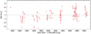 |
Fig. B.1 First 190 HARPS radial velocity measurements of HD 10180. |
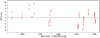 |
Fig. B.2 First 80 HARPS radial velocity measurements of HD 69830. |
Appendix C Marginalisation over linear parameters
C.1 Analytical expressions
Let us consider a model with k planets. The likelihood function is then given by Eq. (A.1) and (A.2). The model (A.3) can be rewritten as

We then re-write Eq. (A.2) in the form
 (C.1)
(C.1)
where η is the vector of non-linear parameters, x is the vector of linear parameters, and Mk is a matrix whose columns include cos νi(t) and sin νi(t), where νi is the true anomaly of planet i, as well as a column with all entries equal to one. The likelihood can then be written
 (C.2)
(C.2)
The evidence of a model with k planets can be split in three integrals, over x, η, and β. When the prior distribution of x p(x) is Gaussian, the integral over x has an analytical expression. In the case where p(x) has a null mean and a covariance matrix Σ, then denoting by N the number of measurements (the dimension of
 (C.3)
(C.3)
 (C.4)
(C.4)
where |X| designates the determinant of a matrix X and
 (C.5)
(C.5)
 (C.6)
(C.6)
 (C.7)
(C.7)
 (C.8)
(C.8)
 (C.9)
(C.9)
A Gaussian prior might be overly restrictive. Fortunately, the analytical formula can be generalised to mixtures of Gaussians. Let us consider a collection of possible covariance matrices (Σi)i=1..M. We suppose that the linear elements x follow a Gaussian of mean 0 and covariance Σi with probability pi and ∑i pi = 1. This prior on x can be seen as a two-step process: (1) selecting a covariance with probability (pi)i·= 1..M, (2) drawing x from a Gaussian with the selected covariance. The prior distribution on x can be written
 (C.10)
where p(x|i) is a Gaussian distribution of mean 0 and covariance Σi· By linearity of the integral,
 (C.11)
where p(y|η,β, k, i) is given by Eq. (C.9) with Σ = Σi.
We specify this general formula to a case that is useful in practice. Let us suppose that for each planet the parameters A and B of equation (C.1) follow a Gaussian mixture model with distributions of standard deviation (σj)j = 1..Q with probabilities qj, with ∑j=1..Q qj = 1. The σj might correspond to different populations (super-Earths, mini-Neptunes, Neptunes, Jupiters). For a given number k of planets, there are Qk combinations of different priors, which can be indexed by i1∈ {1..Q}, i2 ∈ {1..Q}…ik ∈ {1..Q}, that is any combination of k indices with each a value between 1 and Q. For instance, let us suppose that we have a four-planet compact multi-planetary system where planets are a priori either super-Earths or mini-Neptunes. We have a two-component Gaussian mixture model on semi-amplitude with standard deviations σ1 and σ2 and probabilities q1 and q2 = 1 − q1. Then the Gaussian mixture on the linear parameters (Ai,Bi)i·=1..4, where A and B are defined as in eq. (C.1), has 24 = 16 components which can be labelled by the priors chosen on the four planets ranked with increasing period (for each of them, super-Earth or mini-Neptune). In the general case eq. (C.11) becomes
 (C.12)
Here p(y|η, β, k, i1, ….ik) is a Gaussian distribution of covariance matrix  , defined as follows. Ordering the components of x = (A1, B1, ….Ak, Bk, x′), where x' are the linear parameters that do not correspond to a planet, then σ
 (C.13)
When utilising this formula, the number of analytic evaluations of integrals depends exponentially on the number of components in the Gaussian mixture models. However, it might be unnecessary to compute all the Qk components of the model. To illustrate this, let us suppose that Q = 2 and corresponds to Earth-sized and Jupiter-sized planets. If it appears that the likelihood completely excludes a mass above 20 M⊕, then the marginalised likelihood terms involving a Jupiter mass at this period can be neglected.
C.2 Computational time
We tested the advantages of the marginalisation in terms of computational time. We compute the FIP periodogram of the SOPHIE radial velocity data with 179 points spanning 3.2 years, with different assumptions on the prior on A and B in eq. (C.1) or the noise. In the base model the prior on A and B is Gaussian, and the noise model has a free jitter. The calculation is performed with the analytical marginalisation described in Section C.1. We then consider a model including correlated noise with an exponential kernel, such that the noise model is  , where
  , and τ are free parameters. Second, we replace the prior on K with a log-uniform one and a uniform prior on phase. Finally, we use a three-component Gaussian mixture model on A and B and use the analytical marginalisation. We compute as a function of the number of planets in the model how much time it takes to compute the posterior distribution of orbital elements.
In figure C.1 we compare the time it takes to compute the Bayesian evidence with POLYCHORD for each configuration. For the Gaussian mixture model we used three populations, corresponding to super-Earths, sub-Neptunes, and Jupiter-sized planets. We can see that the Gaussian mixture prior and the red noise model are relatively stable between 2 and 5 times slower than the base model, and is systematically faster than a log-uniform prior. The Gaussian mixture model takes more time for a higher number of planets because of the increasing Qk combinations (see eq. (C.12)) that are necessary to compute, even when performing optimisations to remove some of those combinations. On the other hand, when we use a log-uniform prior for the semi-amplitude Κ we see a big increase in computational time, which scales with the number of planets in the model. This is expected as each planet added to the model increases the number of free parameters by three (period, semi-amplitude, and phase) instead of just one (period) when we marginalise over the linear parameters.
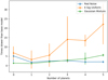 |
Fig. C.1 Runtime comparisons with different assumptions on the model. Plotted are the red noise (blue), log Uniform prior on Κ (orange), and Gaussian mixture prior (green). The y-axis shows the ratio of the average time of the indicated configuration to the average time of the base model. Five independent runs were performed with each number of planets; the mean time is represented with plain lines and the standard deviation is represented as error bars. |
Appendix D Validation tests
In this appendix we list the tests performed to validate our numerical methods. These are built on exactly the same principle as the test performed in Sect. 4.3, but with different input models, which are listed below:
Same priors as Table 1. We generate data on the first 250 HARPS measurement times of HD 69830 instead of the first 80. See Fig. D.1.
Same priors as Table 1 except that systems are generated with 0 to 4 planets See Fig. D.2.
Same priors as Table 1, except that we add a correlated noise with exponential kernel, 1 m/s amplitude, and a decay timescale of 4 days. See Fig. D.3.
Same priors as Table 1, except that orbits are eccentric (uniform argument of periastron) and e is generated from a Beta distribution with a = 0 and b = 15. See Fig. D.4.
Same priors as Table 1, except that orbits are eccentric (uniform argument of periastron) and e is generated from a Beta distribution with a = 0.867 and b = 3.03, as in Kipping (2014). See Fig. D.5.
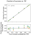 |
Fig. D.1 Fraction of events with probability pj where there actually was a planet injected as a function of pj for the case with 250 measurements instead of 80. |
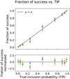 |
Fig. D.2 Fraction of events with probability pj where there actually was a planet injected as a function of pj for the case with up to four planets. |
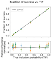 |
Fig. D.3 Fraction of events with probability pj where there actually was a planet injected as a function of pj for the case with correlated noise. |
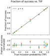 |
Fig. D.4 Fraction of events with probability pj where there actually was a planet injected as a function of pj for the case with eccentric orbits and e generated from a Beta distribution with a = 0 and b = 15. |
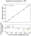 |
Fig. D.5 Fraction of events with probability pj where there actually was a planet injected as a function of pj for the case with eccentric orbits and e generated from a Beta distribution with a = 0.867 and b = 3.03, as in Kipping (2014). |
Appendix E Prior influences
The detection criterion (6) requires us to define priors on the orbital elements. The criterion might favour different detections depending on the priors. We show here that the detections claimed based on (6) and Bayes factors depend on the prior chosen on the semi-amplitude K. We find, loosely speaking, that once the prior encompasses the Κ with high likelihood, the broader the prior on K, the more the addition of a planet in the model is penalised.
This can easily be seen in a simplified setting with the analytical formula (C.4). Let us consider two models with no other components but k and k + 1 planets, and a fixed covariance matrix of the noise V. We further suppose that the models with k and k + 1 planets have specified period, ηk = (P1,…, Pk) and ηk+1 = (P1,…, Pk+1)· Assuming that the prior on the linear parameters A and Β of all the planets (see eq. (C.1)) is Gaussian of null mean and variance L2, then Σ = L2I, where I is the 2k identity matrix. Then (C.4) can be re-written
 (E.1)
(E.1)
 (E.2)
(E.2)
 (E.3)
(E.3)
If we assume that the noise is white of standard deviation σ, denoting by  the χ2 of the least squares estimate fit of Mk with a linear model M and a Gaussian prior on the parameters of mean 0 and covariance Σ, it can be shown that
 (E.4)
(E.4)
The Bayes factor, and thus the strength of the detection increases as the exponential of the χ2 difference of the k + 1 and k model. On the other hand, it is penalised by the denominator term, which accounts for the fact that the evidence of the model with k + 1 planets has a larger parameter space. In the limit of high L which is asymptotically proportional to  .
.
Similarly, considering a flat prior in A and Β on [−L, L], we can easily show that as L grows, the Bayes factor is also proportional to  . For a flat prior in
  on [0, L], the limit is
  . and for a log-uniform prior on Κ on
 ![Mathematical equation: $\left[{{e^{- {L_m}}},{e^{{L_M}}}} \right],{1 \over {\ln \,{L_M} - \ln \,{L_m}}}$](/articles/aa/full_html/2022/07/aa40543-21/aa40543-21-eq69.png) . This behaviour is also apparent in the analysis of Sinharay & Stern (2002), once the prior encompasses the high likelihood region, as it gets wider the Bayes factor favours more and more the simple model.
. This behaviour is also apparent in the analysis of Sinharay & Stern (2002), once the prior encompasses the high likelihood region, as it gets wider the Bayes factor favours more and more the simple model.
References
- Anglada-Escudé, G., & Tuomi, M. 2012, A&A, 548, A58 [NASA ADS] [CrossRef] [EDP Sciences] [Google Scholar]
- Baluev, R.V. 2008, MNRAS, 385, 1279 [NASA ADS] [CrossRef] [Google Scholar]
- Baluev, R.V. 2009, MNRAS, 393, 969 [NASA ADS] [CrossRef] [Google Scholar]
- Baluev, R.V. 2013a, MNRAS, 431, 1167 [NASA ADS] [CrossRef] [Google Scholar]
- Baluev, R.V. 2013b, MNRAS, 436, 807 [NASA ADS] [CrossRef] [Google Scholar]
- Baluev, R.V. 2015, MNRAS, 446, 1478 [NASA ADS] [CrossRef] [Google Scholar]
- Barbieri, M.M., & Berger, J.O. 2004, Ann. Stat., 32, 870 [CrossRef] [Google Scholar]
- Barbieri, M.M., Berger, J.O., George, E.I., & RoCkovâ, V. 2021, Bayesian Anal., 1, 1 [Google Scholar]
- Benjamini, Y., & Hochberg, Y. 1995, J.R. Stat. Soc. B (Methodological), 57, 289 [Google Scholar]
- Boisse, I., Moutou, C., Vidal-Madjar, A., et al. 2009, A&A, 495, 959 [NASA ADS] [CrossRef] [EDP Sciences] [Google Scholar]
- Brewer, B.J. 2014, ArXiv e-prints [arXiv:1411.3921] [Google Scholar]
- Brewer, B.J., & Donovan, C.P. 2015, MNRAS, 448, 3206 [NASA ADS] [CrossRef] [Google Scholar]
- Buchner, J. 2021, ArXiv e-prints, [arXiv:2101.09675] [Google Scholar]
- Casella, G., & Berger, R. 2001, Statistical Inference (Duxbury Resource Center) [Google Scholar]
- Chen, S.S., Donoho, D.L., & Saunders, M.A. 1998, SIAM J. Sci. Comput., 20, 33 [CrossRef] [MathSciNet] [Google Scholar]
- Chib, S., & Kuffner, T.A. 2016, ArXiv e-prints [arXiv:1607.00292] [Google Scholar]
- Collier Cameron, A., Mortier, A., Phillips, D., et al. 2019, MNRAS, 487, 1082 [Google Scholar]
- Cox, R.T. 1946, Am. J. Phys., 14, 1 [NASA ADS] [CrossRef] [Google Scholar]
- Cox, R.T. 1961, The Algebra Of Probable Inference (John Hopkins University Press) [Google Scholar]
- Cumming, A. 2004, MNRAS, 354, 1165 [Google Scholar]
- Cumming, A., Marcy, G.W., & Butler, R.P. 1999, ApJ, 526, 890 [NASA ADS] [CrossRef] [Google Scholar]
- Dawson, R.I., & Fabrycky, D.C. 2010, ApJ, 722, 937 [CrossRef] [Google Scholar]
- Delisle, J.B., Hara, N., & Ségransan, D. 2020, A&A 635, A83 [NASA ADS] [CrossRef] [EDP Sciences] [Google Scholar]
- Draper, D., & Krnjajic, M. 2010, Bayesian Anal., 1, 1 [Google Scholar]
- Dumusque, X., Udry, S., Lovis, C., Santos, N.C., & Monteiro, M.J.P.F.G. 2011, A&A, 525, A140 [NASA ADS] [CrossRef] [EDP Sciences] [Google Scholar]
- Dumusque, X., Boisse, I., & Santos, N.C. 2014, ApJ, 796, 132 [NASA ADS] [CrossRef] [Google Scholar]
- Faria, J.P.D.S. 2018, PhD thesis, Universidade do Porto [Google Scholar]
- Faria, J.P., Haywood, R.D., Brewer, B.J., et al. 2016, A&A, 588, A31 [NASA ADS] [CrossRef] [EDP Sciences] [Google Scholar]
- Faria, J.P., Adibekyan, V., Amazo-Gömez, E.M., et al. 2020, A&A, 635, A13 [NASA ADS] [CrossRef] [EDP Sciences] [Google Scholar]
- Feng, F., Tuomi, M., & Jones, H.R.A. 2017, MNRAS, 470, 4794 [NASA ADS] [CrossRef] [Google Scholar]
- Feroz, F., Balan, S.T., & Hobson, M.P. 2011, MNRAS, 415, 3462 [NASA ADS] [CrossRef] [Google Scholar]
- Ferraz-Mello, S. 1981, AJ, 86, 619 [NASA ADS] [CrossRef] [Google Scholar]
- Ford, E.B. 2005, AJ, 129, 1706 [NASA ADS] [CrossRef] [Google Scholar]
- Ford, E.B. 2006, ApJ, 642, 505 [NASA ADS] [CrossRef] [Google Scholar]
- Ford, E.B., & Gregory, P.C. 2007, in Astronomical Society of the Pacific Conference Series, 371, Statistical Challenges in Modern Astronomy IV, eds. G.J. Babu, & E.D. Feigelson, 189 [NASA ADS] [Google Scholar]
- Fulton, B.J., Petigura, E.A., Howard, A.W., et al. 2017, AJ, 154, 109 [NASA ADS] [CrossRef] [Google Scholar]
- Gaudi, B.S. 2022, The Demographics of Wide-Separation Planets, (Cham: Springer International Publishing), 446, 237 [NASA ADS] [Google Scholar]
- Green, P.J. 1995, Biometrika, 82, 711 [CrossRef] [Google Scholar]
- Gregory, P. 2005, Bayesian Logical Data Analysis for the Physical Sciences (New York: Cambridge University Press) [Google Scholar]
- Gregory, P.C. 2007a, MNRAS, 374, 1321 [NASA ADS] [CrossRef] [Google Scholar]
- Gregory, P.C. 2007b, MNRAS, 381, 1607 [NASA ADS] [CrossRef] [Google Scholar]
- Gregory, P.C. 2016, MNRAS, 458, 2604 [NASA ADS] [CrossRef] [Google Scholar]
- Halpern, J. 1999, Journal of AI research, 10, 67 [Google Scholar]
- Handley, W.J., Hobson, M.P., & Lasenby, A.N. 2015a, MNRAS, 450, L61 [NASA ADS] [CrossRef] [Google Scholar]
- Handley, W.J., Hobson, M.P., & Lasenby, A.N. 2015b, MNRAS, 453, 4384 [Google Scholar]
- Hara, N.C., Boué, G., Laskar, J., & Correia, A.C.M. 2017, MNRAS, 464, 1220 [NASA ADS] [CrossRef] [Google Scholar]
- Hara, N.C., Boué, G., Laskar, J., Delisle, J.B., & Unger, N. 2019, MNRAS, 489, 738 [NASA ADS] [CrossRef] [Google Scholar]
- Hara, N.C., Bouchy, F., Stalport, M., et al. 2020, A&A, 636, A6 [Google Scholar]
- Hara, N.C., de Poyferré, T., Delisle, J.-B., & Hoffmann, M. 2022a, Ann. Appl. Stat., submitted [arXiv:2203.04957] [Google Scholar]
- Hara, N.C., Delisle, J.-B., Unger, N., & Dumusque, X. 2022b, A&A, 658, A177 [NASA ADS] [CrossRef] [EDP Sciences] [Google Scholar]
- Hayashi, C. 1981, Progr. Theor. Phys. Suppl., 70, 35 [Google Scholar]
- Haywood, R.D., Collier Cameron, A., Queloz, D., et al. 2014, MNRAS, 443, 2517 [NASA ADS] [CrossRef] [Google Scholar]
- Haywood, R.D., Collier Cameron, A., Unruh, Y.C., et al. 2016, MNRAS, 457, 3637 [NASA ADS] [CrossRef] [Google Scholar]
- Hobson, M.J., Diaz, R.F., Delfosse, X., et al. 2018, A&A, 618, A103 [NASA ADS] [CrossRef] [EDP Sciences] [Google Scholar]
- Hobson, M.J., Delfosse, X., Astudillo-Defru, N., et al. 2019, A&A, 625, A18 [NASA ADS] [CrossRef] [EDP Sciences] [Google Scholar]
- Hoeting, J.A., Madigan, D., Raftery, A.E., & Volinsky, C.T. 1999, Stat. Sci., 14, 382 [CrossRef] [Google Scholar]
- Hogg, D.W., Myers, A.D., & Bovy, J. 2010, ApJ, 725, 2166 [CrossRef] [Google Scholar]
- Jain, P., Tewari, A., & Dhillon, I.S. 2011, ArXiv e-prints [arXiv:1106.2774] [Google Scholar]
- Jeffreys, H. 1946, Proc. R. Soc. Lond. A: Math. Phys. Eng. Sci., 186, 453 [NASA ADS] [Google Scholar]
- Jeffreys, H. 1961, The Theory of Probability (Oxford University Press) [Google Scholar]
- Jones, D.E., Stenning, D.C., Ford, E.B., et al. 2017, ArXiv e-prints [arXiv:1711.01318] [Google Scholar]
- Kass, R.E., & Raftery, A.E. 1995, J. Am. Stat. Assoc., 90, 773 [Google Scholar]
- Kipping, D.M. 2014, MNRAS, 444, 2263 [NASA ADS] [CrossRef] [Google Scholar]
- Lehmann, E.L., & Romano, J.P. 2005, Testing statistical hypotheses, 3rd edn., Springer Texts in Statistics (New York: Springer) [Google Scholar]
- Leleu, A., Alibert, Y., Hara, N.C., et al. 2021, A&A, 649, A26 [NASA ADS] [CrossRef] [EDP Sciences] [Google Scholar]
- Lomb, N.R. 1976, Ap&SS, 39, 447 [NASA ADS] [CrossRef] [Google Scholar]
- Lovis, C., Mayor, M., Pepe, F., et al. 2006, Nature, 441, 305 [NASA ADS] [CrossRef] [Google Scholar]
- Lovis, C., Ségransan, D., Mayor, M., et al. 2011, A&A, 528, A112 [NASA ADS] [CrossRef] [EDP Sciences] [Google Scholar]
- Meunier, N., Desort, M., & Lagrange, A.-M. 2010, A&A, 512, A39 [NASA ADS] [CrossRef] [EDP Sciences] [Google Scholar]
- Mortier, A., & Collier Cameron, A. 2017, A&A, 601, A110 [NASA ADS] [CrossRef] [EDP Sciences] [Google Scholar]
- Mortier, A., Faria, J.P., Correia, C.M., Santerne, A., & Santos, N.C. 2015, A&A, 573, A101 [NASA ADS] [CrossRef] [EDP Sciences] [Google Scholar]
- Nelson, B.E., Ford, E.B., Buchner, J., et al. 2020, AJ, 159, 73 [NASA ADS] [CrossRef] [Google Scholar]
- Noyes, R.W. 1984, in Space Research in Stellar Activity and Variability, eds. A. Mangeney, & F. Praderie, 113 [Google Scholar]
- O’Toole, S.J., Tinney, C.G., Jones, H.R.A., et al. 2009, MNRAS, 392, 641 [CrossRef] [Google Scholar]
- Paris, J.B. 1994, The Uncertain Reasoner's Companion: A Mathematical Perspective (Cambridge University Press), 4 [Google Scholar]
- Pinamonti, M., Sozzetti, A., Bonomo, A.S., & Damasso, M. 2017, MNRAS, 468, 3775 [CrossRef] [Google Scholar]
- Price-Whelan, A.M., Hogg, D.W., Foreman-Mackey, D., & Rix, H.-W. 2017, ApJ, 837, 20 [NASA ADS] [CrossRef] [Google Scholar]
- Queloz, D., Henry, G.W., Sivan, J.P., et al. 2001, A&A, 379, 279 [NASA ADS] [CrossRef] [EDP Sciences] [Google Scholar]
- Rajpaul, V., Aigrain, S., Osborne, M.A., Reece, S., & Roberts, S.J. 2015, MNRAS, 452, 2269 [NASA ADS] [CrossRef] [Google Scholar]
- Reegen, P. 2007, A&A, 467, 1353 [NASA ADS] [CrossRef] [EDP Sciences] [Google Scholar]
- Robertson, P. 2018, ApJ, 864, L28 [NASA ADS] [CrossRef] [Google Scholar]
- Santerne, A., Malavolta, L., Kosiarek, M.R., et al. 2019, Nat. Astron., submitted, [arXiv:1911.07355] [Google Scholar]
- Scargle, J.D. 1982, ApJ, 263, 835 [NASA ADS] [CrossRef] [Google Scholar]
- Schuster, A. 1898, Terrestrial Magn., 3, 13 [NASA ADS] [CrossRef] [Google Scholar]
- Shannon, C. 1948, Bell Syst. Tech. J., 27 [Google Scholar]
- Shimony, A. 1988, An Adamite Derivation of the Principles of the Calculus of Probability, ed. J.H. Fetzer (Dordrecht: Springer Netherlands), 79 [Google Scholar]
- Sinharay, S., & Stern, H.S. 2002, Am. Stat., 56, 196 [CrossRef] [Google Scholar]
- Soric, B. 1989, J. Am. Stat. Assoc., 84, 608 [Google Scholar]
- Süveges, M. 2014, MNRAS, 440, 2099 [CrossRef] [Google Scholar]
- Tuomi, M. 2011, A&A, 528, L5 [NASA ADS] [CrossRef] [EDP Sciences] [Google Scholar]
- Tuomi, M. 2012, A&A, 543, A52 [NASA ADS] [CrossRef] [EDP Sciences] [Google Scholar]
- Udry, S., Dumusque, X., Lovis, C., et al. 2019, A&A, 622, A37 [NASA ADS] [CrossRef] [EDP Sciences] [Google Scholar]
- van Fraassen, C. 1984, J. Philos., 81, 235 [CrossRef] [Google Scholar]
- Wald, A. 1949, Ann. Math. Stat., 20, 165 [CrossRef] [Google Scholar]
- Wright, J.T., & Howard, A.W. 2009, ApJS, 182, 205 [CrossRef] [Google Scholar]
- Zechmeister, M., & Kürster, M. 2009, A&A, 496, 577 [CrossRef] [EDP Sciences] [Google Scholar]
- Zucker, S. 2015, MNRAS, 449, 2723 [NASA ADS] [CrossRef] [Google Scholar]
- Zucker, S. 2016, MNRAS, 457, L118 [NASA ADS] [CrossRef] [Google Scholar]
- Zucker, S. 2018, MNRAS, 474, L86 [NASA ADS] [CrossRef] [Google Scholar]
The data can be downloaded here: https://dace.unige.ch/radialVelocities/?pattern=HD10180
The ℓ1 periodogram code is available at https://github.com/nathanchara/l1periodogram
All Tables
Parameters of the different runs of POLYCHORD on the HD 10180 dataset, when using a log-uniform prior on semi-amplitude.
Parameters of the different runs of POLYCHORD on the HD 10180 dataset when using a Gaussian mixture prior on semi-amplitude.
All Figures
|
Fig. 1 FIP periodogram of a simulated system with three injected planets. The periods of the peaks are indicated by red points; the −log10FIP and log10TIP are represented as a function of the centre of the period interval considered, in blue and yellow, respectively. |
| In the text | |
|
Fig. 2 Fraction of events with probability pj where there actually was a planet injected as a function of pj. The colours blue, orange and green correspond to different, random choices of events with TIP pj. |
| In the text | |
|
Fig. 3 FIP periodogram of 190 HARPS measurements of HD 10180 computed with a log-uniform prior on semi-amplitude on [0.1, 20] m s−1. In blue: FIP periodogram for up to six planets; in pink: FIP periodogram for up to seven planets. |
| In the text | |
|
Fig. 4 FIP periodogram of 190 HARPS measurements of HD 10180 computed with a log-uniform prior on semi-amplitude on [0.1,20] m s−1. In blue, pink, and green: FIP periodograms corresponding to different runs of calculations of posterior distributions of the parameters of a seven-planet model. |
| In the text | |
|
Fig. 5 FIP periodogram of 190 HARPS measurements of HD 10180 computed with a Gaussian mixture model linear parameters (two components with σ = 1 and 4ms). In blue: FIP periodogram for up to six planets; in pink: FIP periodogram for up to seven planets. |
| In the text | |
|
Fig. 6 FIP periodogram of 190 HARPS measurements of HD 10180 computed with Gaussian mixture model linear parameters (two components with σ = 1 and 4 ms). In blue, pink, and green: FIP periodograms corresponding to different runs of calculations of posterior distributions of the parameters of a seven-planet model. |
| In the text | |
|
Fig. 7 Total number of mistakes on the number of planets (left) and number and period of planets (right) out of 1000 datasets with white noise (simulation 1, see Sect. 6.2.4) as a function of the detection threshold for different statistical significance metrics. From top to bottom: Periodogram + FAP, Periodogram + Bayes factor, ℓ1 periodogram + FAP, and FIP. The total number of false positives and false negatives are represented as light red and blue shaded areas. The false and missed detections are represented in orange and purple shaded areas, respectively. The minimum and maximum values of the detection threshold corresponding to the minimum number of mistakes are indicated with black lines. |
| In the text | |
|
Fig. 7 continued. Same quantities as above, for the detection criteria FIP periodogram + FAP (f1 and f2) and FIP periodogram + Bayes factor (g1 and g2). |
| In the text | |
|
Fig. 8 Number of mistakes as a function of the number of false detections (log scale) for the different detection methods. The number of mistakes is defined as the sum of missed true planets and false detections. The data corresponds to simulation 1 (see Sect. 6.2.4): a random number of planets equal to 0, 1, or 2; the noise is white and Gaussian with semi-amplitude to noise ratio of 3.5. |
| In the text | |
|
Fig. 9 Number of mistakes as a function of the number of false detections (log scale) for the different detection methods. The data corresponds to simulation 2 (see Sect. 6.2.5): a random number of planets equal to 0, 1, or 2 planets per system; white and correlated noise. This simulation has a timescale of 4 days and an amplitude of 1 m s−1. The semi-amplitude to noise level ratio of 1.7. Mistakes are defined as the sum of missed and false detections. |
| In the text | |
|
Fig. 10 Total number of mistakes on the number of planets (left) and number and period of planets (right) out of 1000 datasets with correlated noise (simulation 2, see Sect. 6.2.5) as a function of the detection threshold for different statistical significance metrics. From top to bottom: Periodogram + FAP, Periodogram + Bayes factor, ℓ1 periodogram + FAP and FIP. The total number of false positives and false negatives are represented in light red and blue shaded areas. The false and missed detections are represented in orange and purple shaded areas, respectively. The minimum and maximum values of the detection threshold corresponding to the minimum number of mistakes are marked with black lines. |
| In the text | |
|
Fig. 10 continued. Same quantities as above, for the detection criteria FIP periodogram + FAP (f1 and f2) and FIP periodogram + Bayes factor (g1 and g2). |
| In the text | |
|
Fig. 11 Total number of mistakes (plain line) and total number of false detections (dashed lines) on 1000 simulated systems as a function of the threshold (from top to bottom: periodogram + BF, ℓ1 periodogram and BF, FIP) for different assumptions on the priors (see Sect. 6.3). In blue: correct priors (1.5–100 days log-uniform in period Rayleigh with σ = 1.5 ms−1 on K); in purple: 1.5–10 000 days log-uniform in period; in yellow: Rayleigh with σ = 3m s−1 on K; in red: log-uniform on [0.1, 10] m s−1 on K. The dashed lines represent the number of false detections as a function of the detection threshold and plain lines represent the total number of mistakes (false and missed detection) as a function of the threshold. |
| In the text | |
|
Fig. 12 Number of mistakes (false detection + missed detections) as a function of the number of false detections obtained with the FIP for different priors. The plain lines represent the detections with the FIP and dashed lines with FIP periodograms + Bayes factor. |
| In the text | |
|
Fig. 13 Logarithm (base 10) of Bayes factor comparing models with 1 vs. 0 (blue) and 2 vs. 1 (orange) planets computed on 1000 simulated RV time series (black points). In abscissa the Bayes factor is computed with correct priors. In ordinate, the Bayes factor is computed with identical priors except on period, where the prior width is log-uniform on [1.5, 10 000] days instead of [1.5, 100], The red line represents a linear regression. |
| In the text | |
|
Fig. 14 Priors on semi-amplitude. The red, yellow, and blue curve correspond to Rayleigh priors with σ = 1.5, σ = 3m s−1, and log-uniform on [0.1 – 10]m s−1. The blue dotted line indicates the 0.1m s−1 limit. Shown is the ratio of log-uniform to Rayleigh priors (dashed lines), and of the 1.5 and 3 m s−1 Rayleigh priors (scale is on the right y-axis). |
| In the text | |
|
Fig. 15 Total number of false and missed detections (yellow and purple shaded areas, respectively) on 1000 systems as a function of the FIP threshold when selecting the noise model with a fit of the ancillary indicators. |
| In the text | |
|
Fig. 16 Total number of false and missed detections (yellow and purple shaded areas, respectively) on 1000 systems as a function of the FIP threshold when the noise model is free to vary. |
| In the text | |
|
Fig. 17 Expectancy of the ratio of periodograms computed with a noise with exponential covariance τa and the true timescale τ = 4 days. Each curve corresponds to a different value of τa: 4 days (black) and 1, 2.5, 6, and 8 days (lavender to red). |
| In the text | |
|
Fig. B.1 First 190 HARPS radial velocity measurements of HD 10180. |
| In the text | |
|
Fig. B.2 First 80 HARPS radial velocity measurements of HD 69830. |
| In the text | |
|
Fig. C.1 Runtime comparisons with different assumptions on the model. Plotted are the red noise (blue), log Uniform prior on Κ (orange), and Gaussian mixture prior (green). The y-axis shows the ratio of the average time of the indicated configuration to the average time of the base model. Five independent runs were performed with each number of planets; the mean time is represented with plain lines and the standard deviation is represented as error bars. |
| In the text | |
|
Fig. D.1 Fraction of events with probability pj where there actually was a planet injected as a function of pj for the case with 250 measurements instead of 80. |
| In the text | |
|
Fig. D.2 Fraction of events with probability pj where there actually was a planet injected as a function of pj for the case with up to four planets. |
| In the text | |
|
Fig. D.3 Fraction of events with probability pj where there actually was a planet injected as a function of pj for the case with correlated noise. |
| In the text | |
|
Fig. D.4 Fraction of events with probability pj where there actually was a planet injected as a function of pj for the case with eccentric orbits and e generated from a Beta distribution with a = 0 and b = 15. |
| In the text | |
|
Fig. D.5 Fraction of events with probability pj where there actually was a planet injected as a function of pj for the case with eccentric orbits and e generated from a Beta distribution with a = 0.867 and b = 3.03, as in Kipping (2014). |
| In the text | |
Current usage metrics show cumulative count of Article Views (full-text article views including HTML views, PDF and ePub downloads, according to the available data) and Abstracts Views on Vision4Press platform.
Data correspond to usage on the plateform after 2015. The current usage metrics is available 48-96 hours after online publication and is updated daily on week days.
Initial download of the metrics may take a while.