| Issue |
A&A
Volume 662, June 2022
|
|
|---|---|---|
| Article Number | A14 | |
| Number of page(s) | 11 | |
| Section | The Sun and the Heliosphere | |
| DOI | https://doi.org/10.1051/0004-6361/202243169 | |
| Published online | 31 May 2022 | |
First detection of metric emission from a solar surge⋆
1
Department of Physics, University of Ioannina, 45110 Ioannina, Greece
e-mail: This email address is being protected from spambots. You need JavaScript enabled to view it.
2
Section of Astrophysics, Astronomy & Mechanics, Department of Physics, University of Athens, Panepistimiopolis 157 84, Zografos, Greece
Received:
21
January
2022
Accepted:
1
March
2022
Abstract
We report the first detection of metric radio emission from a surge, observed with the Nançay Radioheliograph (NRH), STEREO, and other instruments. The emission was observed during the late phase of the M9 complex event SOL2010-02-012T11:25:00, described in a previous publication. It was associated with a secondary energy release, also observed in STEREO 304 Å images, and there was no detectable soft X-ray emission. The triangulation of the STEREO images allowed for the identification of the surge with NRH sources near the central meridian. The radio emission of the surge occurred in two phases and consisted of two sources, one located near the base of the surge, apparently at or near the site of energy release, and another in the upper part of the surge; these were best visible in the frequency range of 445.0 to about 300 MHz, whereas a spectral component of a different nature was observed at lower frequencies. Sub-second time variations were detected in both sources during both phases, with a 0.2–0.3 s delay of the upper source with respect to the lower, suggesting superluminal velocities. This effect can be explained if the emission of the upper source was due to scattering of radiation from the source at the base of the surge. In addition, the radio emission showed signs of pulsations and spikes. We discuss possible emission mechanisms for the slow time variability component of the lower radio source. Gyrosynchrotron emission reproduced the characteristics of the observed total intensity spectrum at the start of the second phase of the event fairly well, but failed to reproduce the high degree of the observed circular polarization or the spectra at other instances. On the other hand, type IV-like plasma emission from the fundamental could explain the high polarization and the fine structure in the dynamic spectrum; moreover, it gives projected radio source positions on the plane of the sky, as seen from STEREO-A, near the base of the surge. Taking all the properties into consideration, we suggest that type IV-like plasma emission with a low-intensity gyrosynchrotron component is the most plausible mechanism.
Key words: Sun: radio radiation / Sun: UV radiation / Sun: activity / Sun: corona / Sun: flares
Movie associated to Fig. A.2 is available at https://www.aanda.org
© ESO 2022
1. Introduction
Solar electromagnetic radiation extends from γ-rays to km wavelengths. Each spectral range provides specific information on solar phenomena, whereas combined observations in many spectral ranges are required to obtain a complete picture of physical processes operating in the solar atmosphere. Solar radio emission, in particular, which originates from the low chromosphere at mm-wavelengths up to the outer corona and the solar wind at km wavelengths, covers the same altitude range as emissions in the optical, EUV, and X-ray ranges as well as in the in situ measurements; hence, it is a necessary complement of data obtained in these domains (see, e.g., the recent review from Alissandrakis 2020).
Practically all phenomena observed in radio wavelengths have their counterpart in other regions of the electromagnetic spectrum. Metric solar bursts are an exception to the above statement. Although we have a basic understanding of their origin, some of their counterparts in other spectral ranges have not been identified. For example, we know that type III bursts are due to beams of accelerated electrons but such beams are not detectable in optical or EUV wavelengths, although they have been observed by particle detectors in the interplanetary space. Similarly, we know that type II bursts are due to shock waves, but we are not sure which observable manifestation of the shocks corresponds to the radio emission. The reason for this lies apparently in the fact that both type IIs and type IIIs result from coherent plasma emission, which has no observable signature outside the radio range.
The only definitive association between metric burst and optical/EUV emission is that of the so called “radio CMEs,” emitting in the radio range through the incoherent gyrosynchrotron mechanism (see, e.g., Bastian et al. 2001; Maia et al. 2007; Démoulin et al. 2012; Tun & Vourlidas 2013; Bain et al. 2014; Carley et al. 2017; Mondal et al. 2020; Chhabra et al. 2021; see also Sect. 5 in Alissandrakis & Gary 2020). This gyrosynchrotron emission originates at the core of the CME, as one of the components of the radio signature that appear on dynamic spectra in the form of a type IV continuum (see Chhabra et al. 2021, for example); additional components of this kind of type IV burst due to plasma radiation (Vasanth et al. 2019; Morosan et al. 2019) are also possible.
There have also been reports of soft X-ray (SXR) jets associated with Type III emission, apparently from accelerated electrons that traveled along the path outlined by the jet (Kundu et al. 1995; Raulin et al. 1996a). Moreover, Raulin et al. (1996b) reported the occurrence of a metric continuum source that was associated with both the partial rupture of a coronal loop top and soft X-ray plasma ejecta, whereas Kundu et al. (2001) reported the detection of metric continuum sources associated with soft X-ray plasmoid ejecta. Earlier works (Axisa et al. 1973, Mein & Avignon 1985, Chiuderi-Drago et al. 1986) reported the association of Type IIIs with Hα ejecta, in particular surges. However, no direct emission from the SXR or optical structures themselves were reported by the above authors, with the possible exception of Raulin et al. (1996b).
We note that “jet” is a generic term that may describe material ejections of various natures, including surges. The latter, classically, are ejections of chromospheric material, best observed in Hα beyond the limb; they are usually seen in absorption on the disk and occasionally in emission (Zirin 1966, 1988; Roy 1973). Contrary to sprays, the motion of the material in surges is ordered and appears to follow the magnetic field lines of force, while the material often comes back along the same path.
The development of soft X-ray, ultraviolet (UV), and extreme ultraviolet (EUV) instrumentation has helped to identify ejecta in these wavelength ranges as well. They are usually called jets and their properties have been reviewed by Raouafi et al. (2016). It appears that in several cases, the ejected material is multi-thermal, which allows for the detection of its cool, dense component in Hα as a surge and the detection of its hotter, more tenuous component in (E)UV or soft X-rays as a jet. Using Interface Region Imaging Spectrograph (IRIS) data and numerical simulations, Nóbrega-Siverio et al. (2021) have found that surges are characterized by temperatures around 6000 K at −6.0 ≤ log10(τ)≤ − 3.2 and electron densities ranging from 1.6 × 10¹¹ up to about 1012 cm−3 at −6.0 ≤ log10(τ)≤ − 4.8. On the other hand, in soft X-rays and the EUV, the temperature of jets may exceed 2 MK while their density can reach values as high as 109–1010 cm−3 (e.g., Mulay et al. 2016). Atmospheric Imaging Assembly (AIA) observations of a surge at 304 Å yielded an average density of 4.1×109 cm−3 (Kayshap et al. 2013).
There is a long tradition of interpreting jets and surges as a result of magnetic reconnection between newly emerged magnetic flux and the preexisting coronal magnetic field (e.g., Shibata et al. 1992; Yokoyama & Shibata 1995, 1996; Archontis & Hood 2008, 2012, 2013; Moreno-Insertis & Galsgaard 2013). Observations of jets associated with the eruption of small-scale filaments (e.g., Sterling et al. 2015, 2016) has led Wyper et al. (2017, 2018) to propose that the ejected material is generated by a break-out mechanism similar to the one that might be at work in the initiation of CMEs (Antiochos et al. 1999).
In a previous work (Alissandrakis et al. 2021, hereafter Paper I), we presented a detailed analysis of the complex M9 event SOL2010-02-012T11:25:00, whose dynamic spectrum contained at least five lanes of type-II emission and included a surge, a CME and an EUV wave. Our analysis showed that the type IIs were not associated with the surge but, rather, with the EUV wave that had probably been initiated by the surge. During the main phase of the event, there was no detectable metric emission from the surge.
In this article, we report the detection of surge-associated emission that occurred after the end of the bulk of the metric radio burst. In the next section, we present our observations and in Sect. 3, our results. In Sect. 4, we discuss possible emission mechanisms, whereas in Sect. 5, we present our conclusions. Finally in Appendix A, we give the full dynamic spectrum of the event and a movie of images used in this study.
2. Observations and data analysis
The data set used in this work is similar to the one used for Paper I, for the time interval 11:45 to 13:00 UT of February 12, 2010. In short, we used images from the Nançay Radioheliograph (Kerdraon & Delouis 1997, NRH)1; dynamic spectra from the ARTEMIS-JLS radiospectrograph (Caroubalos et al. 2001; Kontogeorgos et al. 2006) and CALLISTO2; light curves from the Geostationary Operational Environmental Satellite (GOES); Hα images from Catania Observatory; soft X-ray images from the GOES Soft X-ray Imager (SXI); EUV images at 304 Å with a cadence of 10 min from the STEREO Sun-Earth Connection Coronal and Heliospheric Investigation (SECCHI) Ahead and Behind and coronograph images from STEREO Coronagraph1 (COR1) A and B (Howard et al. 2008), with a cadence of 5 min. No Solar and Heliospheric Observatory (SOHO) Extreme ultraviolet Imaging Telescope (EIT) data were available during the event, while the Transition Region and Coronal Explorer (TRACE) was pointed elsewhere.
The NRH provided data at ten frequencies (150.9, 173.2, 228.0, 270.6, 298.7, 327.0, 360.8, 408.0, 432.0, and 445.5 MHz), with a cadence of 250 ms and a spatial resolution of 1.2′ by 1.8′ at 432 MHz. For a global view of the event, we used 10 s average images, whereas for a detailed study we used images with the full temporal resolution. To facilitate displays and comparisons, we also computed cuts of intensity as a function of time and position, along the axis of the surge. Three-dimensional positions were computed from triangulation of STEREO A and B 304 Å images, as well as from COR1 images.
3. Results
3.1. Overview
The GOES class M9 event, which occurred around 11:25 UT on February 12, 2010 in active region 11046, was described in detail in Paper I. The bulk of the radio emission ended around 11:32 UT (see Fig. 1 of Paper I), but metric continuum emission appeared again in the dynamic spectrum from about 12:00 to 13:00 UT (see Fig. 45 of Bouratzis et al. 2015, reproduced in Fig. A.1). This continuum was associated with the second phase of the surge described in this work.
In the STEREO images, the surge started around 11:23 UT and was visible in the 304 Å band well after the main metric emission, till about 13:26 UT. In the 195 Å band it was visible in emission up to about 11:38 UT, whereas the top of the surge went above the COR1 A and B occulting disks at around 11:40 UT.
Seen from STEREO-A, the event was very close to the E limb, whereas it was near the W limb for STEREO-B (Fig. 1). Figure 2 shows a sequence of STEREO-A images, in which the surge is very prominent as it is seen mostly beyond the limb. We note that between 11:36 and 11:46 UT a second ejection of material occurred, as noted in Paper I (Sect. 3.2 and Fig. 5), where it was characterized as a “slow component”. For comparison, we also show a pair of STEREO A and B 304 Å images in Fig. 3, where the points used for triangulation are marked.
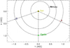 |
Fig. 1. Positions of the STEREO spacecrafts on February 12, 2010. |
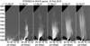 |
Fig. 2. Base difference images of the surge in the 304 Å band, as seen from STEREO-A. The intensity is given as a function of position angle and distance from the center of the disk. The solar radius is 972″. |
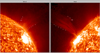 |
Fig. 3. STEREO-B (left) and A (right) images of the surge in the 304 Å band at 11:56 UT. The crosses mark the triangulation points. |
Radio emission from the surge was detected by the NRH during two intervals: from 11:49 to 11:51 UT (phase A) and from 12:00 to ∼13:00 UT (phase B). Figure 4 shows NRH total intensity images during both phases, together with Hα and SXR images. The corresponding circular polarization images are shown in Fig. 5.
 |
Fig. 4. NRH images in total intensity (Stokes parameter I) of the surge at all ten frequencies during the first (top) and the second (bottom) phase of the event. The white arc marks the solar limb, the insert shows the NRH beam (resolution), while the cross-hair is placed at the maximum of the lower source at 445 MHz during the first phase. The images are normalized so that the maximum intensity at each frequency is white and the minimum is black, with a linear scale (γ = 1.). An Hα image from Catania and a long exposure SXR image from SXI are given for reference in the left column. |
 |
Fig. 5. NRH images for circular polarization (Stokes V). Here, a short exposure SXI image is given in the lower left panel, to show better the structure of the active region and zero V is gray. |
We first note that there is no trace of surge emission either in Hα or in SXR. We further note that in both phases two sources appear in the high-frequency images where the resolution is higher; moreover, during phase B the upper source is clearly displaced upwards, compared to phase A, which is apparently a result of the expansion of the surge. A final remark at this stage is that the size and position of the source are markedly different in the two lowest frequencies, indicating different structures or different emission mechanisms. This is further corroborated by an inspection of the V images, which show a bipolar structure at low frequencies that is more prominent during phase B. On the other hand, at high frequencies, both the lower and the upper source were uniformly polarized in the right-hand sense.
3.2. Low time-resolution analysis
At the full cadence (250 ms) of the NRH, our 65 min of data at ten frequencies and two Stokes parameters make a total of 312 000 images. This is a huge number of images, which cannot be easily treated. For this reason, we start our analysis with 10 s average images which preserve the basic characteristics of the event while reducing the number of images by a factor of 40.
3.2.1. Evolution in time
Even at the reduced time resolution, the number of images is still high. A convenient way of presentation is through cuts of the intensity as a function of position and time, which are displayed in Fig. 6. The full set of averaged images is presented in Movie 1 of the Appendix (see Fig. A.2).
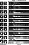 |
Fig. 6. Cuts of intensity as a function of time and position along the surge axis from 10 s resolution NRH total intensity images. Zero position is at the middle of the cut. Corresponding images during the first phase and the beginning of the second phase of the surge are given on the left of the cuts; dashed vertical lines mark the limits of the cut region. The width of the cut changes with frequency in order to cover the entire emitting region. A and B in the 445.0 MHz cut mark the two phases of the event. We note that phase A was much shorter and weaker than phase B. |
The cuts confirm our previous conclusion that the nature of the source is different at the two low frequencies; indeed, the cuts at 173.2 and 150.9 MHz show fluctuating emission but no concrete sign of the two phases. Moreover, the cuts provide some additional interesting information:
The emission during phase B was much brighter and longer than the emission during phase A. In addition, the duration of this phase increased as the frequency decreased, and extended beyond 13:00 UT. The emission from the lower source during the same phase can roughly be split in three parts, best visible at high frequencies: from 12:00 to 12:15 UT, from 12:15 UT to 12:28 UT, and beyond 12:28 UT.
The visibility of the upper source decreased with decreasing frequency. In order to check whether this is due to the NRH resolution, we convolved the 445 MHz image with the beam of all other frequencies, after deconvolving with the 445 MHz beam. We found that the upper source should be detectable even at 150.9 MHz, during phase B, in particular, where the two sources are further apart. This means that the intensity of the upper source, relative to the intensity of the lower source, increases with frequency.
3.2.2. Positions and motions
As mentioned above, the three-dimensional position of surge features were computed from triangulation of STEREO A and B images. From these, the projection of the surge on the plane of the sky, as seen from the Earth, was computed and is displayed in Fig. 7. The position (centroid), as well as the brightness temperature and size of the radio sources was computed by Gaussian fit of their images. The positions derived from 10 s average images at 432.0 MHz during the entire event are plotted as dots in Fig. 7, black for the lower source and red for the upper. The flare position, from XRT and Catania images, is shown as an open circle in the same figure (see also Fig. 6 in Paper I).
 |
Fig. 7. Positions of various components of the surge derived from triangulation of STEREO images, on the plane of the sky as seen from the Earth. The positions of the radio sources at 432.0 MHz are shown as black and red dots, for the lower and upper components of the emission respectively. The open circle shows the location of the flare. Straight lines are from linear regression. The black arc marks the solar limb. |
A first remark is that the surge was huge, its projected length being about a solar radius around 12:00 UT. On the average, its position angle was about 34° east of north. The radio source positions were spread along a shorter, but still quite long structure, going as far as the low part of COR1A emission. The extent of radio emission was about 0.5 R⊙, and was displaced by about 150 ″ to the west of the surge; this displacement is comparable to the observed width of the sources and might be due to refraction or scattering effects or triangulation errors. We note that the orientation of the radio source motion was close to that of the surge, about 29°.
From the position of the top of the surge in STEREO-A 304 Å images, we deduced an accelerating motion and we obtained a velocity, projected on the plane of the sky, of about 126 km s−1 around 12:00 UT; this is consistent with the value of 120 km s−1, obtained from COR1A measurements in Paper I (Sect. 3.2) for this component of the surge. Since, according to our triangulation the surge was inclined by about 15° with respect to the plane of the sky as seen from STEREO-A, this velocity translates to 130 km s−1 along the surge direction. On the other hand, a linear regression of the positions of the upper NRH source at 445.0 MHz as a function of time gave an apparent velocity of 123 km s−1. Seen from the Earth, the inclination of the surge with respect to the plane of the sky was 45° (see Fig. 8 below) and this value corresponds to 175 km s−1 along the surge. Although this value is ∼35% above the one deduced from the limb measurements, it is probably more reliable since the source centroids can be more accurately identified and measured than the diffuse top of the 304 Å images. We note that the upward displacement of the lower source (black dots in Fig. 7) is considerably smaller (≃40 km s−1) than that of the upper source (red dots). This is expected, since the material in the lower source is continuously replenished from the eruption that produced the surge.
 |
Fig. 8. Positions of the surge components derived from triangulation of STEREO images, on a plane perpendicular to the plane of the sky. The open circle shows the location of the flare. Straight lines are from linear regression. The black arc marks the solar limb. |
Putting together all information presented in this section, there can be no doubt that what we see from the Earth at metric wavelengths is indeed emission associated with the 304 Å surge seen near the limb from STEREO A and B.
In order to complete the picture, we provide in Fig. 8 the surge positions, derived from triangulation, projected on a plane that includes the line of sight. Apart from providing the inclination of the surge with respect to the plane of the sky as seen from the Earth, the plot shows a change of the surge inclination with height, apparently reflecting the curved shape of this structure seen in Fig. 2.
3.3. Intensity fluctuations from full time-resolution data
Although our 10 s average images give an accurate view of the structure and the evolution of the event, there is a lot more of information in the full time sequence of NRH images that are explored in this section, individually for phases A and B.
3.3.1. Phase A
The first phase of the metric surge emission was rather short, lasting for about 2 min. A concise picture of its structure and evolution is given in the total intensity cuts (Fig. 9) at the three highest NRH frequencies, where the two sources were clearly resolved. The circular polarization cuts show a similar picture and are not shown here.
 |
Fig. 9. Stokes I cuts (intensity as a function of time and position along the surge), at full time resolution, for 445.0, 432.0, and 408.0 MHz, during phase A of the surge. Zero position is at the middle of the cut. The width of the cuts is marked on the images at left. |
The time variation in the cuts of Fig. 9 reveals two temporal components of the emission: one with a timescale on the order of 1 min and a second, fluctuating component, with sub-second scale. A power spectrum analysis did not reveal any concrete periodicities in the fluctuations, which occurred at an average rate of about one per second.
The long timescale component is broadband and detectable from 445.0 MHz down to about 298.7 MHz, whereas most fluctuations are very different in the consecutive NRH channels displayed in the figure, which puts an upper limit of a few tens of MHz in their bandwidth. Still, there are some short time scale structures in the 408.0–298.7 MHz frequency range, which are visible in more than one NRH channel, suggesting a bandwidth of the order of 100 MHz; this is shown in Fig. 10, where a high-pass Gaussian filter of 5 s width has been applied to the cuts in order to enhance fine structures.
 |
Fig. 10. High-pass time filtered Stokes I cuts, for 408.0, 360.8, 327.0, and 298,7 MHz. The width of the cuts is marked on the images at left. |
Most interesting, the pattern of fluctuations is very similar in the two sources, with a slight time delay of 0.2 s of the upper source with respect to the lower, as measured through cross-correlation of their light curves; this appears as a small inclination in the cuts of Fig. 9. Taken literally, this translates to an apparent superluminal propagation speed of 2.6c on the plane of the sky, the projected distance of the two sources being about 230″. As the geometry has to be fully taken into consideration, we come back to this issue in Sect. 4.
As expected, the light curves of the two sources follow closely each other for all three frequencies considered here (Fig. 11). The time shift between the two sources is also visible in this figure and so is the narrow bandwidth of the fluctuations. The brightness temperature, Tb, of the lower source is of the order of 107 K. At 445.0 MHz the brightness of the upper source is slightly lower than that of the lower source, their ratio being 0.85; this value decreases to 0.60 at 432.0 MHz and to 0.38 at 408.0 MHz. This quantifies our previous remark (Sect. 3.2.1) that the visibility of the upper source decreased with decreasing frequency. Finally, there appears to be no association of the radio emission to the GOES soft x-ray flux.
 |
Fig. 11. Light curves of brightness temperature for the three frequencies shown in Fig, 9. The GOES light curve is also shown for reference, where the straight line marks the linear fit of the background. |
3.3.2. Phase B
As mentioned earlier, phase B was much longer and more intense than phase A (cf. Fig. 6). The upper source is now detectable in the four higher NRH frequencies, fading as time progresses; it is further away from the lower source, a consequence of the expansion of the surge. As it is impossible to present its time evolution in full, we show in Fig. 12 the first 3.5 min.
 |
Fig. 12. Stokes I cuts at full time resolution, for 445.0, 432.0, 408.0, and 360.8 MHz, during phase B of the surge. Zero position is at the middle of the cut. The width of the cuts is marked on the images at left. |
As in phase A, the intensity shows short time scale fluctuations; however, their coherence between the upper and lower sources is much reduced, particularly after 12:02 UT. Until then, the fluctuations in the upper source were delayed by 0.3 s, 50% more than during phase A; the increased delay is apparently related to the increased separation of the two sources.
Figure 13 compares the light curves of the upper and lower sources, computed from the 1D cuts. No GOES curve is given, as there was no SXR emission. Contrary to phase A, the intensity of the upper source not only is about a factor of 5 lower than that of the lower source, but it also decreases with time. This decrease could be associated with the increase of the distance between the two sources or the fading of the upper part of the surge.
 |
Fig. 13. Light curves at full time resolution, for 445.0, 432.0, 408.0, and 360.8 MHz, during phase B of the surge. Intensity scales for the lower and upper sources are different by a factor of 5. |
3.4. Spectrum and polarization
The average spectrum of the surge, computed from the peak NRH brightness temperature during phase A, is displayed in the upper panel of Fig. 14. The low and high-frequency spectral components discussed previously are clearly identifiable, with a cross-over frequency around 270 MHz. We note that the high-frequency component, which is the one directly associated with the burst, is rather flat with a peak around 432 MHz (Tb ≃ 15 MK).
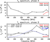 |
Fig. 14. Brightness temperature spectra during phase A (time average, top panel) and during phase B (2 instances, bottom). The Tb scales in the two panels differ by a factor of 10. The blue dotted curve in the lower panel shows a fit of the high-frequency part of the spectrum with a gyrosynchrotron model discussed in Sect. 4.2. |
During phase B both the low and the high-frequency spectral components brightened, the latter more than the former; they are still distinguished in the spectrum (lower panel of Fig. 14) and all the better in the early stage of phase B (dashed line). The high-frequency component now shows a prominent peak around 360 MHz, whose brightness temperature exceeds 150 MK. We note that in both phases the emission appears to extend beyond the highest NRH frequency of 445 MHz.
With ten NRH channels between 150.9 and 445 MHz, it is possible to try to construct a dynamic spectrum that would give more complete spectro-temporal information. Such a “pseudo dynamic spectrum” is presented in the top panel of Fig. 15. It compares well with the e-Callisto dynamic spectrum of Bleien Observatory (BLEN7M). The flux was below the detection threshold of other radiospectrographs, including ARTEMIS-JLS. Unfortunately the Bleien spectrum showed a sharp drop above 450 MHz, apparently of instrumental origin as it appeared in all dynamic spectra from this instrument and, thus, we cannot estimate the high-frequency extent of the emission.
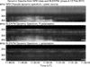 |
Fig. 15. Dynamic spectra during phase A of the surge from NRH imaging data (top) and from e-Callisto of Bleien Observatory in right and left circular polarization (middle and bottom) in the frequency range 150–525 MHz. Horizontal line segments at left and at right mark the NRH frequencies. The time interval is the same as in Fig. 9. |
Features of different temporal and frequency scales (cf. Sect. 3.3) are well visible in both spectra. In particular, repeated short duration spectral features visible down to ∼300 MHz do not show any appreciable drift and they might be some sort of pulsations. The BLEN7M spectra in Fig. 15 reveal a very high degree of circular polarization in the right-hand sense, which is confirmed by the NRH images that give a degree of polarization above 80%.
Similarly, Fig. 16 shows dynamic spectra during the second phase of the emission. In addition to the discrete low- and high-frequency components, these spectra clearly show pulsations, well visible in the BLEN7M spectrum of the middle panel. Moreover, after the application of a high pass time filter of 12 s width, the spectrum obtained with the ARTEMIS-JLS acousto-optic analyzer (SAO) shows spike-like structures (bottom panel in the figure).
 |
Fig. 16. Dynamic spectra from 12:00 to 12:06:20 UT, near the start of phase B of the surge from NRH imaging data (top), from e-Callisto of Bleien Observatory in right circular polarization (middle) and from the acousto-optic analyzer of ARTEMIS-JLS (bottom, subjected to high pass time filtering). Fringe-like patterns in the bottom panel are of instrumental origin. |
4. Discussion
4.1. Apparent superluminal velocities
The apparent superluminal velocities deduced from the delay of fluctuations between the upper and lower sources during phase A (Sect. 3.3.1) and the start of phase B (Sect. 3.3.2) point towards the possibility that the emission of the upper source is scattered radiation from the lower source. In this section, we explore this possibility.
The relevant geometry is shown in Fig. 17. In deducing the 3D positions of the NRH sources, we assumed that the upper source was located in the middle of the region defined by the edges of the 304 Å surge, as derived from triangulation (red symbols and lines in Fig. 17). For the lower source, we assumed that it was located lower, at a height of 1.03 R⊙, consistent with the computations in the next section. Then the delay between emission from the lower source and scattered emission from the upper source is:
 (1)
(1)
 |
Fig. 17. NRH source positions on a plane perpendicular to the sky plane (open circles). A and B refer to the corresponding phases of the emission. The limits of the 304 Å surge derived from triangulation are also plotted in red for reference (cf. Fig. 8). Dotted lines with arrows point towards the observer. The black arc marks the solar limb. |
and, taking into account the geometry, we have:
 (2)
(2)
For phase A, the geometry gives θ ≃ 24°, whereas Δx ≃ 230″ = 165 Mm, hence:
 (3)
(3)
which is compatible with the measured delay of 0.2 s.
Similarly, for the start of phase B we have θ ≃ 31° and Δx≃ 236 Mm, thus:
 (4)
(4)
which is again compatible with the observed delay of 0.30 s. We note that the assumed height of the lower source does not affect much the results; a greater height would increase θ slightly and decrease Δt.
We conclude that scattering of the emission from the lower source by the upper is a plausible interpretation of the apparent superluminal velocity. This conclusion is further strengthened by the decrease of the upper to lower intensity ratio with time, both between the two phases, as well as during phase B: it is a natural consequence of the increasing distance between the two sources, to which we may add the decrease of the density of the surge as it expands. The observed decrease of the upper to lower source intensity ratio at lower frequencies may imply that the scattering is more efficient at high frequencies.
4.2. Emission mechanism
Having established that the emission of the upper source was due to scattering from the lower source, which was located at or near the site of energy release, we focus on the emission mechanism of the latter, in particular to its high-frequency component (⪆270 MHz), which was directly associated with the surge. Noting also that pulsations and spike-like features were present in this emission, we consider only the component with slow time variations. In this section we discuss all three possible emission mechanisms: thermal emission, gyrosynchrotron, and plasma.
It is well known (e.g., see review in Nindos 2020) that in flare events, the heated coronal plasma becomes optically thick to thermal free-free emission below about 10 GHz. In such a case, the brightness temperature can reach values exceeding 107 K, its spectrum is flat and the degree of circular polarization is low (⪅10%). In our case, the lower source exhibits flat spectra during phase A from 327 to 408 MHz (top panel of Fig. 14) and during phase B in the interval 12:01–12:03 UT from 408 to 432 MHz (dashed line of bottom panel of Fig. 14). However, the degree of circular polarization is higher than 80% throughout the event which rules out the interpretation in terms of free-free emission. More importantly, there was not any surge-associated emission in the GOES data (Sect. 3.3), whereas the SXR emission had dropped to preflare levels during the time interval that we consider here (see Fig. 2 of Paper I), which precludes the presence of high temperature plasma; this also rules out the possibility of thermal gyroresonance emission.
We went on to investigate whether gyrosynchrotron radiation from nonthermal electrons is at the heart of the emission. To this end, we first attempted to model the high-frequency part of the spectrum from 12:01–12:03 UT in the early part of phase B (dashed line in the bottom panel of Fig. 14) with a gyrosynchrotron spectrum. We used the inhomogeneous gyrosynchrotron code described in Nindos et al. (2000, see also Kundu et al. 2004; Tzatzakis et al. 2008) with the addition that the effects of the ambient medium were taken into account, in order to properly account for the Razin-Tsytovich suppression (e.g., Razin 1960; Klein 1987; Melnikov et al. 2008) at low frequencies.
We constrained our models by fixing both the source angular scale and line-of-sight length to 200″, in agreement with the results from the Gaussian fit to the radio images (see Sect. 3.2). These fits showed that the source size did not change appreciably with frequency, which justifies our decision to work with the brightness temperature spectra instead of the flux density spectra. The remaining fit parameters are the energy spectral index, δ, of the energetic electrons, the magnetic field, B, the low- and high-energy cutoffs, E1 and E2, respectively, of the nonthermal electrons, their density, Nr, and the density of the ambient thermal plasma, N0. The parameterized gyrosynchrotron model was fit to the spectrum using the Leveberg-Marquardt least-squares method. The best-fit model parameters, as well as their uncertainties, are given in Table 1.
Best-fit model gyrosynchrotron parameters.
Our model gyrosynchrotron spectrum is shown as the blue dotted line in Fig. 14. This model yields brightness temperatures which are broadly consistent with those observed from 270 to 445 MHz. However, the model degree of circular polarization ranges from 40% to 70% in the optically thin part of the spectrum whereas observations indicate that it is higher than 80%. The discrepancy is even worse at 270.6 and 298.7 MHz, falling into the optically thick part of the spectrum, where the model gives a degree of circular polarization as low as 25%. It is possible to adjust the fit parameters to make the model polarization approach the observed one in the optically thin frequencies, at the cost of both unmatched total intensity brightness temperatures (differences of more than a factor of 4) and the shift of the peak emission to about 400 MHz.
The characteristics of the phase B spectrum from 12:05 to 12:10 UT (full line of the bottom panel of Fig. 14), particularly the higher brightness temperature and spectral peak around 360 MHz, are difficult to reproduce using any plausible combination of gyrosynchrotron model input parameters. The same is true for the spectrum of phase A (top panel of Fig. 14), which shows an extended flat region at high frequencies that we could not reconcile with gyrosynchrotron models.
Using the gyrosynchrotron model parameters, we can place constraints on the energetics of the surge. From the density of the ambient thermal plasma (1.5 × 108 cm−3) and the maximum height and speed of the surge of this study, ≈0.5 R⊙ and 130 km s−1, respectively, we found a surge mechanical (kinetic+potential) energy density of ≈0.02 erg cm−3. The model magnetic field strength of the surge in the 5–35 G range gives a magnetic energy density of ≈1–49 erg cm−3, which is more than sufficient to balance the mechanical energy density. This finding is consistent with a magnetic driving of the observed surge. We reached the same result by employing the density of the surge reported in (Kayshap et al. 2013) (i.e., 4.1 × 109 cm−3), leading to a surge mechanical energy density of ≈0.6 erg cm−3, still short of the magnetic energy density. We note that, in contrast to the study of Kayshap et al. (2013), we were not able to derive the density from the differential emission measure, since our data set lacked simultaneous multi-channel observations of the surge.
We now turn to the plasma mechanism. The observed high degree of circular polarization is consistent with plasma emission from the fundamental. It is well known that plasma emission is a leading candidate for type IV bursts (see Nindos et al. 2008, and references therein). In several cases (see, e.g., Bouratzis et al. 2015), these bursts exhibit fine structures that are similar to those detected in the dynamic spectrum of this surge (Figs. 15 and 16). We note that type IV emissions come with a variety of bandwidths, and sometimes do not extend below 250 MHz (see events 17 and 20 in Bouratzis et al. 2015), as is the case with the present event. Therefore, an interpretation in terms of type IV plasma emission could be consistent with these aspects of our event.
Under the hypothesis of emission at the fundamental, the height of the radio sources can be computed. Based on this, their projected position above the limb as seen from STEREO-A can be deduced and compared with the surge images at 304 Å. The results are displayed in Fig. 18, for the two phases of the radio emission. The computation was performed for an isothermal coronal model at 2 × 10⁶ K and a base electron density 3.5 times that of the Newkirk model. We note that the projected positions are close to the base of the 304 Å surge, which adds strength to the type IV interpretation. Our choice of the density multiplication factor, k, took into account the fact that for k < 3 the 445 MHz level is below the photosphere; going to k = 4 gives a height difference of 15 Mm, which would still put the NRH source near the base of the 304 Å surge.
 |
Fig. 18. Computed NRH source positions from 327 to 435 MHz (red filled circles) projected on the sky plane as seen from STEREO-A, on top of base-difference 304 Å images near phase A (left) and during phase B (right). Higher-frequency sources are at lower radial distances. |
5. Summary and conclusions
In this work, we report the detection of metric radio emission from a surge, associated with a secondary energy release during the late phase of the M9 event of February 12, 2010 that was previously analyzed in Paper I. Although there have been earlier reports of metric emission associated with SXR jets, this is the first time that direct imaging of a surge has been reported.
The surge was imaged by STEREO A and B, seen near the east and west limbs, respectively. Although no optical or EUV observations near the Earth were available and nothing was detected in SXR images, the identification of the NRH emission with the surge was established with confidence from triangulation of STEREO 304 Å and COR1 images. Moreover, consistent expansion velocities on the order of 150 km s−1 were measured based on the NRH and STEREO data. We note that no surge-associated emission was detected during the main phase of that event, apparently due to its low brightness temperature and the limited dynamic range of the NRH.
The metric emission consisted of two spectral components, a high-frequency component definitely associated with the surge and a low frequency one of different nature, with a crossover around 270 MHz. The high-frequency component developed in two phases, A and B, with phase B much longer and brighter than phase A; moreover, it consisted of two radio sources, one near the base of the surge (lower source) and one in the upper part (upper source) during both phases. The separation of these sources increased over time, reflecting the expansion of the surge, while the intensity of the upper source decreased compared to that of the lower one.
Both sources showed short timescale variations, narrow-band and broad-band. There was a high degree of coherence between the upper and the low source during phase A and the beginning of phase B, with a delay of the upper source by 0.2 and 0.3 s for A and B, respectively. Although, at a first glance, this delay suggests superluminal velocities, a proper consideration of the geometry revealed that scattering of radiation from the lower source by the upper source is the most likely explanation. This scattering is more efficient at higher frequencies.
The two spectral components and the presence of short time scale fluctuations were confirmed in dynamic spectra, constructed from the ten frequency channels of the NRH (“pseudo dynamic spectra”) as well as from the e-Callisto instrument of the Bleien Observatory and from ARTEMIS-JLS. They all show signs of pulsations and spike-like emission, in addition to the continuum components.
Taking into account all available information, we examined possible emission mechanisms of the high-frequency component of the lower source, which was apparently located at or near the site of energy release. The morphology of the total intensity spectra, the high degree of circular polarization, and the absence of strong SXR emission rule out an interpretation in terms of thermal mechanisms.
The lower source total intensity spectrum during phase B from 12:01 to 12:03 UT was reproduced fairly well by a model of gyrosynchrotron emission from mildly relativistic electrons with energy cutoffs of 5 and 150 keV and density of 6.1 × 106 cm−3 radiating in magnetic fields with strengths ranging from 5 to 35 G. However, this model yields degrees of polarization that are lower than the observed ones: 40–70% in the optically thin part of the spectrum and even lower in the optically thick part, versus the observed > 80%. Attempts to fix this problem at high frequencies impacted the overall match between the observed and model spectrum, whereas the degree of circular polarization mismatch persisted at low frequencies. At other time intervals, the disagreement between observations and gyrosynchrotron models was even worse.
We note that the parameters of the gyrosynchrotron model lead to the plausible conclusion that the energy stored in the magnetic field of the surge is sufficient to balance mechanical energy losses – a result that points toward a magnetic driver for the surge. We add that even if gyrosynchrotron emission occurred for a short time interval only, the derived physical parameters and the energetics based on them would still reflect the actual situation.
It appears that the observed high degree of circular polarization, as well as the presence of spikes and pulsations in the dynamic spectrum, could be accommodated by plasma emission from the fundamental. Moreover, radio source positions computed under this mechanism are consistent with the surge position as seen from STEREO-A. Hence, we consider type IV-like plasma emission with a low intensity gyrosynchrotron component as the most plausible mechanism.
The detection of surge-associated emission adds one more manifestation to the list of flare-associated metric radio emissions. More observations of this kind will help establish its characteristics and the nature of the emission.
Movie
Movie 1 associated with Fig. A.2 (10s) Access Supplementary Material
Downloaded from http://secchirh.obspm.fr/
Downloaded from http://soleil.i4ds.ch/solarradio/callistoQuicklooks/
Acknowledgments
The authors wish to thank the radio monitoring service at LESIA (Observatoire de Paris) for providing data used for this study, in particular our colleagues from the Observatoire de Paris-Meudon and the NRH staff, as well as the rest of the ARTEMIS-JLS group. Data from CALLISTO, GOES, NOAA and STEREO were obtained from the respective data bases; we are grateful to all those who contributed to the operation of these instruments and made the data available to the community.
References
- Alissandrakis, C. E. 2020, Front. Astron. Space Sci., 7, 74 [NASA ADS] [CrossRef] [Google Scholar]
- Alissandrakis, C., & Gary, D. E. 2020, Front. Astron. Space Sci., 7, 77 [NASA ADS] [CrossRef] [Google Scholar]
- Alissandrakis, C. E., Nindos, A., Patsourakos, S., & Hillaris, A. 2021, A&A, 654, A112 (Paper I) [NASA ADS] [CrossRef] [EDP Sciences] [Google Scholar]
- Antiochos, S. K., DeVore, C. R., & Klimchuk, J. A. 1999, ApJ, 510, 485 [Google Scholar]
- Archontis, V., & Hood, A. W. 2008, ApJ, 674, L113 [Google Scholar]
- Archontis, V., & Hood, A. W. 2012, A&A, 537, A62 [NASA ADS] [CrossRef] [EDP Sciences] [Google Scholar]
- Archontis, V., & Hood, A. W. 2013, ApJ, 769, L21 [Google Scholar]
- Axisa, F., Martres, M. J., Pick, M., et al. 1973, Sol. Phys., 29, 163 [NASA ADS] [CrossRef] [Google Scholar]
- Bain, H. M., Krucker, S., Saint-Hilaire, P., & Raftery, C. L. 2014, ApJ, 782, 43 [Google Scholar]
- Bastian, T. S., Pick, M., Kerdraon, A., Maia, D., & Vourlidas, A. 2001, ApJ, 558, L65 [Google Scholar]
- Bouratzis, C., Hillaris, A., Alissandrakis, C. E., et al. 2015, Sol. Phys., 290, 219 [NASA ADS] [CrossRef] [Google Scholar]
- Carley, E. P., Vilmer, N., Simões, P. J. A., & Ó Fearraigh, B. 2017, A&A, 608, A137 [NASA ADS] [CrossRef] [EDP Sciences] [Google Scholar]
- Caroubalos, C., Maroulis, D., Patavalis, N., et al. 2001, Exp. Astron., 11, 23 [NASA ADS] [CrossRef] [Google Scholar]
- Chhabra, S., Gary, D. E., Hallinan, G., et al. 2021, ApJ, 906, 132 [NASA ADS] [CrossRef] [Google Scholar]
- Chiuderi-Drago, F., Mein, N., & Pick, M. 1986, Sol. Phys., 103, 235 [NASA ADS] [CrossRef] [Google Scholar]
- Démoulin, P., Vourlidas, A., Pick, M., & Bouteille, A. 2012, ApJ, 750, 147 [Google Scholar]
- Howard, R. A., Moses, J. D., Vourlidas, A., et al. 2008, Space Sci. Rev., 136, 67 [NASA ADS] [CrossRef] [Google Scholar]
- Kayshap, P., Srivastava, A. K., Murawski, K., & Tripathi, D. 2013, ApJ, 770, L3 [NASA ADS] [CrossRef] [Google Scholar]
- Kerdraon, A., & Delouis, J.-M. 1997, in The Nançay Radioheliograph, ed. G. Trottet, 483, 192 [Google Scholar]
- Klein, K. L. 1987, A&A, 183, 341 [NASA ADS] [Google Scholar]
- Kontogeorgos, A., Tsitsipis, P., Caroubalos, C., et al. 2006, Exp. Astron., 21, 41 [NASA ADS] [CrossRef] [Google Scholar]
- Kundu, M. R., Raulin, J. P., Nitta, N., et al. 1995, ApJ, 447, L135 [NASA ADS] [Google Scholar]
- Kundu, M. R., Nindos, A., Vilmer, N., et al. 2001, ApJ, 559, 443 [NASA ADS] [CrossRef] [Google Scholar]
- Kundu, M. R., Nindos, A., & Grechnev, V. V. 2004, A&A, 420, 351 [NASA ADS] [CrossRef] [EDP Sciences] [Google Scholar]
- Maia, D. J. F., Gama, R., Mercier, C., et al. 2007, ApJ, 660, 874 [NASA ADS] [CrossRef] [Google Scholar]
- Mein, N., & Avignon, Y. 1985, Sol. Phys., 95, 331 [NASA ADS] [CrossRef] [Google Scholar]
- Melnikov, V. F., Gary, D. E., & Nita, G. M. 2008, Sol. Phys., 253, 43 [NASA ADS] [CrossRef] [Google Scholar]
- Mondal, S., Oberoi, D., & Vourlidas, A. 2020, ApJ, 893, 28 [NASA ADS] [CrossRef] [Google Scholar]
- Moreno-Insertis, F., & Galsgaard, K. 2013, ApJ, 771, 20 [Google Scholar]
- Morosan, D. E., Kilpua, E. K. J., Carley, E. P., & Monstein, C. 2019, A&A, 623, A63 [NASA ADS] [CrossRef] [EDP Sciences] [Google Scholar]
- Mulay, S. M., Tripathi, D., Del Zanna, G., & Mason, H. 2016, A&A, 589, A79 [NASA ADS] [CrossRef] [EDP Sciences] [Google Scholar]
- Nindos, A. 2020, Front. Astron. Space Sci., 7, 57 [NASA ADS] [CrossRef] [Google Scholar]
- Nindos, A., White, S. M., Kundu, M. R., & Gary, D. E. 2000, ApJ, 533, 1053 [NASA ADS] [CrossRef] [Google Scholar]
- Nindos, A., Aurass, H., Klein, K. L., & Trottet, G. 2008, Sol. Phys., 253, 3 [NASA ADS] [CrossRef] [Google Scholar]
- Nóbrega-Siverio, D., Guglielmino, S. L., & Sainz Dalda, A. 2021, A&A, 655, A28 [CrossRef] [EDP Sciences] [Google Scholar]
- Raouafi, N. E., Patsourakos, S., Pariat, E., et al. 2016, Space Sci. Rev., 201, 1 [Google Scholar]
- Raulin, J. P., Kundu, M. R., Hudson, H. S., Nitta, N., & Raoult, A. 1996a, A&A, 306, 299 [NASA ADS] [Google Scholar]
- Raulin, J. P., Kundu, M. R., Nitta, N., & Raoult, A. 1996b, ApJ, 472, 874 [NASA ADS] [CrossRef] [Google Scholar]
- Razin, V. A. 1960, Izv. Vys. Ucheb. Zav. Radiofiz., 3, 584 [Google Scholar]
- Roy, J. R. 1973, Sol. Phys., 28, 95 [NASA ADS] [CrossRef] [Google Scholar]
- Shibata, K., Ishido, Y., Acton, L. W., et al. 1992, PASJ, 44, L173 [Google Scholar]
- Sterling, A. C., Moore, R. L., Falconer, D. A., & Adams, M. 2015, Nature, 523, 437 [NASA ADS] [CrossRef] [Google Scholar]
- Sterling, A. C., Moore, R. L., Falconer, D. A., et al. 2016, ApJ, 821, 100 [CrossRef] [Google Scholar]
- Tun, S. D., & Vourlidas, A. 2013, ApJ, 766, 130 [Google Scholar]
- Tzatzakis, V., Nindos, A., & Alissandrakis, C. E. 2008, Sol. Phys., 253, 79 [NASA ADS] [CrossRef] [Google Scholar]
- Vasanth, V., Chen, Y., Lv, M., et al. 2019, ApJ, 870, 30 [Google Scholar]
- Wyper, P. F., Antiochos, S. K., & DeVore, C. R. 2017, Nature, 544, 452 [Google Scholar]
- Wyper, P. F., DeVore, C. R., & Antiochos, S. K. 2018, ApJ, 852, 98 [Google Scholar]
- Yokoyama, T., & Shibata, K. 1995, Nature, 375, 42 [Google Scholar]
- Yokoyama, T., & Shibata, K. 1996, PASJ, 48, 353 [Google Scholar]
- Zirin, H. 1966, The Solar Atmosphere (Waltham, Mass: Blaisdell) [Google Scholar]
- Zirin, H. 1988, Astrophysics of the Sun (Cambridge: University Press) [Google Scholar]
Appendix A: Supplementry material
A.1. Full dynamic spectrum
Fig. A.1 shows the entire dynamic spectrum of the February 12, 2010 event (cf. Fig. 45 of Bouratzis et al. 2015). The emission before 11:33 UT is from the main event described in Paper I (cf. Fig. 1 in Alissandrakis et al. 2021), with the 2 type IIs and numerous type IIIs. The emission after 12:00 UT is from phase B of the surge, whereas emission from phase A was below the threshold of the instrument.
 |
Fig. A.1. Low time-resolution dynamic spectrum of the entire event in the long decimetric-metric range from 11:24 to 12:58 UT. Dashed horizontal lines mark the NRH frequencies. |
A.2. Movie with 10 s average NRH images
Fig. A.2 shows two frames from Movie 1, which includes all 10 s averaged NRH images in the interval from 11:45 to 13:00 UT, for both the total intensity (Stokes parameter I) and circular polarization (Stokes parameter V). The intensity as a function of time and position along the surge at 445 MHz is shown in the bottom frame, with the vertical line marking the time of the images.
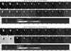 |
Fig. A.2. Two frames of Movie 1, during phase A and at the beginning of phase B. Each frame shows radio images at all ten NRH frequencies in total intensity (top row) and circular polarization (middle row). The color table of each image is such that the maximum intensity is white and the minimum intensity is black. The instrumental beam is shown in the low left corner, while the white circle marks the photospheric limb. In the bottom row a cut of the intensity along the surge as a function of position and time is given, where the white vertical line marks the time of the images. |
All Tables
All Figures
|
Fig. 1. Positions of the STEREO spacecrafts on February 12, 2010. |
| In the text | |
|
Fig. 2. Base difference images of the surge in the 304 Å band, as seen from STEREO-A. The intensity is given as a function of position angle and distance from the center of the disk. The solar radius is 972″. |
| In the text | |
|
Fig. 3. STEREO-B (left) and A (right) images of the surge in the 304 Å band at 11:56 UT. The crosses mark the triangulation points. |
| In the text | |
|
Fig. 4. NRH images in total intensity (Stokes parameter I) of the surge at all ten frequencies during the first (top) and the second (bottom) phase of the event. The white arc marks the solar limb, the insert shows the NRH beam (resolution), while the cross-hair is placed at the maximum of the lower source at 445 MHz during the first phase. The images are normalized so that the maximum intensity at each frequency is white and the minimum is black, with a linear scale (γ = 1.). An Hα image from Catania and a long exposure SXR image from SXI are given for reference in the left column. |
| In the text | |
|
Fig. 5. NRH images for circular polarization (Stokes V). Here, a short exposure SXI image is given in the lower left panel, to show better the structure of the active region and zero V is gray. |
| In the text | |
|
Fig. 6. Cuts of intensity as a function of time and position along the surge axis from 10 s resolution NRH total intensity images. Zero position is at the middle of the cut. Corresponding images during the first phase and the beginning of the second phase of the surge are given on the left of the cuts; dashed vertical lines mark the limits of the cut region. The width of the cut changes with frequency in order to cover the entire emitting region. A and B in the 445.0 MHz cut mark the two phases of the event. We note that phase A was much shorter and weaker than phase B. |
| In the text | |
|
Fig. 7. Positions of various components of the surge derived from triangulation of STEREO images, on the plane of the sky as seen from the Earth. The positions of the radio sources at 432.0 MHz are shown as black and red dots, for the lower and upper components of the emission respectively. The open circle shows the location of the flare. Straight lines are from linear regression. The black arc marks the solar limb. |
| In the text | |
|
Fig. 8. Positions of the surge components derived from triangulation of STEREO images, on a plane perpendicular to the plane of the sky. The open circle shows the location of the flare. Straight lines are from linear regression. The black arc marks the solar limb. |
| In the text | |
|
Fig. 9. Stokes I cuts (intensity as a function of time and position along the surge), at full time resolution, for 445.0, 432.0, and 408.0 MHz, during phase A of the surge. Zero position is at the middle of the cut. The width of the cuts is marked on the images at left. |
| In the text | |
|
Fig. 10. High-pass time filtered Stokes I cuts, for 408.0, 360.8, 327.0, and 298,7 MHz. The width of the cuts is marked on the images at left. |
| In the text | |
|
Fig. 11. Light curves of brightness temperature for the three frequencies shown in Fig, 9. The GOES light curve is also shown for reference, where the straight line marks the linear fit of the background. |
| In the text | |
|
Fig. 12. Stokes I cuts at full time resolution, for 445.0, 432.0, 408.0, and 360.8 MHz, during phase B of the surge. Zero position is at the middle of the cut. The width of the cuts is marked on the images at left. |
| In the text | |
|
Fig. 13. Light curves at full time resolution, for 445.0, 432.0, 408.0, and 360.8 MHz, during phase B of the surge. Intensity scales for the lower and upper sources are different by a factor of 5. |
| In the text | |
|
Fig. 14. Brightness temperature spectra during phase A (time average, top panel) and during phase B (2 instances, bottom). The Tb scales in the two panels differ by a factor of 10. The blue dotted curve in the lower panel shows a fit of the high-frequency part of the spectrum with a gyrosynchrotron model discussed in Sect. 4.2. |
| In the text | |
|
Fig. 15. Dynamic spectra during phase A of the surge from NRH imaging data (top) and from e-Callisto of Bleien Observatory in right and left circular polarization (middle and bottom) in the frequency range 150–525 MHz. Horizontal line segments at left and at right mark the NRH frequencies. The time interval is the same as in Fig. 9. |
| In the text | |
|
Fig. 16. Dynamic spectra from 12:00 to 12:06:20 UT, near the start of phase B of the surge from NRH imaging data (top), from e-Callisto of Bleien Observatory in right circular polarization (middle) and from the acousto-optic analyzer of ARTEMIS-JLS (bottom, subjected to high pass time filtering). Fringe-like patterns in the bottom panel are of instrumental origin. |
| In the text | |
|
Fig. 17. NRH source positions on a plane perpendicular to the sky plane (open circles). A and B refer to the corresponding phases of the emission. The limits of the 304 Å surge derived from triangulation are also plotted in red for reference (cf. Fig. 8). Dotted lines with arrows point towards the observer. The black arc marks the solar limb. |
| In the text | |
|
Fig. 18. Computed NRH source positions from 327 to 435 MHz (red filled circles) projected on the sky plane as seen from STEREO-A, on top of base-difference 304 Å images near phase A (left) and during phase B (right). Higher-frequency sources are at lower radial distances. |
| In the text | |
|
Fig. A.1. Low time-resolution dynamic spectrum of the entire event in the long decimetric-metric range from 11:24 to 12:58 UT. Dashed horizontal lines mark the NRH frequencies. |
| In the text | |
|
Fig. A.2. Two frames of Movie 1, during phase A and at the beginning of phase B. Each frame shows radio images at all ten NRH frequencies in total intensity (top row) and circular polarization (middle row). The color table of each image is such that the maximum intensity is white and the minimum intensity is black. The instrumental beam is shown in the low left corner, while the white circle marks the photospheric limb. In the bottom row a cut of the intensity along the surge as a function of position and time is given, where the white vertical line marks the time of the images. |
| In the text | |
Current usage metrics show cumulative count of Article Views (full-text article views including HTML views, PDF and ePub downloads, according to the available data) and Abstracts Views on Vision4Press platform.
Data correspond to usage on the plateform after 2015. The current usage metrics is available 48-96 hours after online publication and is updated daily on week days.
Initial download of the metrics may take a while.