| Issue |
A&A
Volume 662, June 2022
|
|
|---|---|---|
| Article Number | A107 | |
| Number of page(s) | 21 | |
| Section | Planets and planetary systems | |
| DOI | https://doi.org/10.1051/0004-6361/202142883 | |
| Published online | 28 June 2022 | |
TOI-1268b: The youngest hot Saturn-mass transiting exoplanet
1
Astronomical Institute, Czech Academy of Sciences,
Fričova 298,
251 65
Ondřejov,
Czech Republic
e-mail: This email address is being protected from spambots. You need JavaScript enabled to view it.
2
Astronomical Institute of Charles University,
V Holešovičkách 2,
180 00
Prague,
Czech Republic
3
ESO,
Karl-Schwarzschild-Straße 2,
85748
Garching bei München,
Germany
4
Department of Astronomy, The University of Texas at Austin,
Austin,
TX
78712,
USA
5
Center for Planetary Systems Habitability, The University of Texas at Austin,
Austin,
TX
78712,
USA
6
Thueringer Landessternwarte Tautenburg,
Sternwarte 5,
07778
Tautenburg,
Germany
7
McDonald Observatory, The University of Texas at Austin,
Austin,
TX
78712,
USA
8
Dipartimento di Fisica, Università degli Studi di Torino,
via Pietro Giuria 1,
10125
Torino,
Italy
9
Centre for Astronomy and Astrophysics, Technical University Berlin,
10585
Berlin,
Germany
10
Institute of Planetary Research, German Aerospace Center (DLR),
Rutherfordstraße 2,
12489
Berlin,
Germany
11
Vanderbilt University, Department of Physics & Astronomy,
6301 Stevenson Center Ln.,
Nashville,
TN
37235,
USA
12
Fisk University, Department of Physics,
1000 18th Ave. N.,
Nashville,
TN
37208,
USA
13
Instituto de Astrofísica de Canarias (IAC),
Calle Vía Láctea s/n,
38205
La Laguna,
Tenerife,
Spain
14
Departamento de Astrofísica, Universidad de La Laguna (ULL),
38205
La Laguna,
Tenerife,
Spain
15
Department of Space, Earth and Environment, Chalmers University of Technology, Onsala Space Observatory,
439 92
Onsala,
Sweden
16
Rheinisches Institut für Umweltforschung an der Universität zu Köln,
Aachener Strasse 209,
50931
Köln,
Germany
17
Department of Theoretical Physics and Astrophysics, Masaryk University,
Kotlářská 2,
61137
Brno,
Czech Republic
18
Astronomy Department, University of California,
Berkeley,
CA
94720,
USA
19
California Institute of Technology,
Pasadena,
CA
91125,
USA
20
Department of Physics and Kavli Institute for Astrophysics and Space Research, Massachusetts Institute of Technology,
Cambridge,
MA
02139,
USA
21
Mullard Space Science Laboratory, University College London,
Holmbury St Mary, Dorking,
Surrey
RH5 6NT,
UK
22
Space Telescope Science Institute,
3700 San Martin Drive,
Baltimore,
MD
21218,
USA
23
Leiden Observatory, Leiden University,
NL-2333 CA
Leiden,
The Netherlands
24
NASA Ames Research Center,
Moffett Field,
CA
94035,
USA
25
Department of Space, Earth and Environment, Astronomy and Plasma Physics, Chalmers University of Technology,
412 96
Gothenburg,
Sweden
26
Department of Astronomy, University of Tokyo,
7-3-1 Hongo,
Bunkyo-ku,
Tokyo
113-0033,
Japan
27
Astrobiology Center,
2-21-1 Osawa, Mitaka,
Tokyo
181-8588,
Japan
28
National Astronomical Observatory of Japan,
2-21-1 Osawa, Mitaka,
Tokyo
181-8588,
Japan
29
Instituto de Astrofísica de Andalucía (IAA-CSIC),
Glorieta de la Astronomía s/n,
18008
Granada,
Spain
30
NCCR/Planet-S, Universität Bern,
Gesellschaftsstrasse 6,
3012
Bern,
Switzerland
31
Astronomy Department and Van Vleck Observatory, Wesleyan University,
Middletown,
CT
06459,
USA
32
Department of Earth, Atmospheric and Planetary Sciences, Massachusetts Institute of Technology,
Cambridge,
MA
02139,
USA
33
Department of Aeronautics and Astronautics,
MIT, 77 Massachusetts Avenue,
Cambridge,
MA
02139,
USA
Received:
10
December
2021
Accepted:
16
February
2022
Abstract
We report the discovery of TOI-1268b, a transiting Saturn-mass planet from the TESS space mission. With an age of less than 1 Gyr, derived from various age indicators, TOI-1268b is the youngest Saturn-mass planet known to date; it contributes to the small sample of well-characterised young planets. It has an orbital period of P = 8.1577080 ± 0.0000044 days, and transits an early K-dwarf star with a mass of M* = 0.96 ± 0.04 M⊙, a radius of R* = 0.92 ± 0.06 R⊙, an effective temperature of Teff = 5300 ± 100 K, and a metallicity of 0.36 ± 0.06 dex. By combining TESS photometry with high-resolution spectra acquired with the Tull spectrograph at the McDonald Observatory, and the high-resolution spectrographs at the Tautenburg and Ondřejov Observatories, we measured a planetary mass of Mp = 96.4 ± 8.3 M⊕ and a radius of Rp = 9.1 ± 0.6 R⊕. TOI-1268 is an ideal system for studying the role of star-planet tidal interactions for non-inflated Saturn-mass planets. We used system parameters derived in this paper to constrain the planet’s tidal quality factor to the range of 104.5–5.3. When compared with the sample of other non-inflated Saturn-mass planets, TOI-1268b is one of the best candidates for transmission spectroscopy studies.
Key words: techniques: spectroscopic / techniques: radial velocities / techniques: photometric / planetary systems / planets and satellites: gaseous planets / planets and satellites: atmospheres
© ESO 2022
1 Introduction
After the initial discovery phase, the focus of exoplanet research is now shifting to the detailed studies of the formation and evolution of planets and their atmospheres. Transiting close-in giant planets are crucial to this research because it is easier to characterise them compared to smaller planets orbiting at large distances from their host stars. One process that affects the evolution of planetary atmospheres is atmospheric erosion. Haswell et al. (2012), Staab et al. (2017), and others have shown that substantial atmospheric erosion is ongoing in a large fraction of exoplanets.
Planetary atmospheres can be eroded via hydrodynamic escape caused by the X-ray+EUV (XUV) radiation of the host star. As summarised by Perryman (2018), the hydrodynamic escape rate scales with the flux of the XUV radiation that the planet receives. Since the XUV flux of young stars is orders of magnitude larger than for older ones, the main erosion phase happens in the first 300–500 Myr for planets orbiting solar-like stars. Because of the loss of angular momentum, mainly by stellar wind, the rotation rate, and thus the activity level and its XUV flux, declines with age (Tu et al. 2015). Planets around stars younger than about 1 Gyr are ideal targets for studying the erosion of planetary atmospheres. Gas giants with a relatively low mass but a relatively large radius are particularly interesting because the erosion rate scales with the planet’s surface gravity. However, only six of them orbit stars younger than 1 Gyr: Kelt-9 (Gaudi et al. 2017), Kelt-17 (Zhou et al. 2016), WASP-178 (Rodríguez Martínez et al. 2020), Mascara-4 (Dorval et al. 2020), AU Mic (Plavchan et al. 2020; Martioli et al. 2021), and V1298 Tau (Suárez Mascareño et al. 2021; Poppenhaeger et al. 2021).
Giant planets are believed to form via core accretion in a protoplanetary disc at distances greater than 0.5 au from the host stars (Wuchterl et al. 2000). Such scales provide an environment with enough solid material and gas for the core to become sufficiently massive to start accreting gas and ends up as a giant planet. The giant planet may then migrate inwards according to the initial conditions (Coleman et al. 2017). During migration, the star-planet tidal interaction plays a role in the further evolution of these gas giants, making their orbits circularised and synchronised with the host star’s rotation period (Hut 1980; Rasio & Ford 1996; Pont 2009). The timescales of these processes can help understand the formation and evolution path of individual systems (Weiss et al. 2017; Persson et al. 2019). However, this is strongly limited by uncertainties of tidal quality factors for planets and stars that are complicated to measure. This problem was discussed in Šubjak et al. (2020), who were not able to precisely assess how the system was formed because of the difficulty in measuring tidal interactions. Even so, systems that are too young to be circularised and synchronised can be used to study tidal interactions and put constraints on the tidal quality factors.
Finally, close-in gas giant planets with large radii but relatively low masses that orbit bright stars are also ideal targets for atmospheric studies. The atmospheric signature of a planet is easier to detect if it has a large scale height, which depends on the temperature and surface gravity of the planet. Such planets are ideal targets for the ESA atmospheric characterisation mission Atmospheric Remote-sensing Infrared Exoplanet Large-survey (ARIEL; Tinetti et al. 2016, 2018). ARIEL will observe 1000 preselected transiting planets, of which 50–100 will be studied intensively. The best targets for ARIEL observations are planets that are relatively warm and that orbit relatively bright stars.
Here we report a new result from the KESPRINT consortium (e.g. Van Eylen et al. 2021; Luque et al. 2021; Šubjak et al. 2020; Fridlund et al. 2020; Persson et al. 2019): the discovery of TOI-1268b, a Saturn-mass planet orbiting a young early K-dwarf star that is an ideal target for studying atmospheric erosion and tidal interactions.
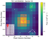 |
Fig. 1 Gaia DR2 catalogue overplotted to the TESS TPF image. |
2 Observations
2.1 TESS photometry
TESS observed TOI-1268 as part of the four Sectors 15, 21, 22, and 41. All observations were performed in the two-minute cadence mode. TESS will further observe TOI-1268 in Sectors 48 and 49. The publicly available data for TOI-1268 can be found in the Mikulski Archive for Space Telescopes (MAST)1, and are provided by the TESS Science Processing Operations Center (SPOC). The transit signature of TOI-1268b was detected by both the SPOC (Jenkins et al. 2016) and the Quick-Look Pipeline (QLP; Huang et al. 2020a,b) pipelines and alerted by the TESS Science Office on Oct. 17, 2019 (Guerrero et al. 2021).
We used the lightkurve package (Lightkurve Collaboration 2018) to download the TESS target pixel files (Fig. 1) from the MAST archive directly. We then selected the optimal aperture masks to obtain light curves (LCs) for each sector, which we normalised and corrected for outliers. We did not use the LCs processed by the SPOC pipeline (Jenkins et al. 2016), which in addition removes the systematics of the spacecraft, as the algorithm removed one transit in Sector 15 and one transit in Sector 22. The missing transits were gapped due to scattered light features by photometric analysis (PA), which in this case appears to have been too aggressive. The SPOC pipeline also analyses the crowding using the Pixel Response Functions (PRFs) and includes a crowding correction in the PDC_SAP flux time series. Not considering such a correction can lead to underestimating the planet’s radius. However, the pipeline indicates that 0.9995 of the light in the optimal aperture is due to the target rather than other stellar sources, suggesting the insignificant dilution due to the faint background stars. Additionally, the analysis of Sectors 14–41 included a difference image centroiding analysis by data validation (Twicken et al. 2018) that indicated the source of the transit signature was within 0.375 ± 2.500 arcsec of the target star.
To correct for the systematics and remove stellar variability, we used the Python package citlalicue (Barragán et al. 2022) to detrend the normalised LCs extracted with lightkurve. The citlalicue package uses a Gaussian process regression as well as transit models computed with the pytransit code (Parviainen 2015) to generate a model that contains both the variability in the LC and the transits. The variability is then removed to leave a flattened LC with only the transit photometric variations. In this case, the variability removed contains both stellar activity and systematics. The LCs before and after the procedure are shown in Fig. 2. Together 15 transits were detected, four each in Sectors 15, 22, 41, and three in Sector 21.
Additionally, we used tpfplotter (Aller et al. 2020) to overplot the Gaia DR2 catalogue to the TESS target pixel file (tpf) in order to identify any possible diluting sources in the TESS photometry, up to a limiting magnitude difference of ten. The tpf image created with tpfplotter can be seen in Fig. 1. We identified two additional sources between TESS pixels diluting TESS LCs. These stars are listed in Table 1. With a magnitude difference greater than eight, these sources are too faint compared to TOI-1268 to yield any significant dilution. The basic parameters of the star are listed in Table 2.
Additional sources within the TESS aperture.
2.2 Ground-based photometry
As part of the TESS Follow-up Observing Program (TFOP), we collected ground-based photometric data of TOI-1268. The observations were scheduled using Transit Finder, a customised version of the Tapir software (Jensen 2013), and photometric data were extracted using AstroImageJ (Collins et al. 2017). In a few cases only part of the transit is observed, while in others the LC precision is too low to hope to improve the parameters from the TESS LCs. Hence, we do not further consider ground-based photometry in this paper.
2.3 High-resolution imaging
To ensure that there are no diluting sources (closer than the Gaia separation limit of 0.4″), high-resolution images were obtained, using adaptive optics and speckle imaging.
On February 02, 2021, TOI-1268 was observed with the Alopeke speckle imager (Scott & Howell 2018) mounted on the 8.1 m Gemini-North telescope. Alopeke uses high-speed iXon Ultra 888 back-illuminated electron multiplying CCDs (EMC-CDs) to simultaneously acquire data in two bands centred around 562 and 832 nm. The data were reduced following the procedures in Howell et al. (2011) and the final reconstructed image, shown in Fig. 3, reaches a contrast of ∆mag = 6.36 at a separation of 0.5″ in the 832 nm band and ∆mag = 4.47 at a separation of 0.5″ in the 562 nm band. The estimated PSF is 0.02″ wide. At the distance of TOI-1268, the star appears single within a separation from 10 to 130 au with contrasts between 5 and 7.5 mag in the 832 nm band.
On January 08, 2020, TOI-1268 was observed using the Palomar High Angular Resolution Observer (PHARO; Hayward et al. 2001) with the JPL Palomar Adaptive Optics System, mounted on the 5.0 m Hale telescope. PHARO uses a 1024 × 1024 HAWAII HgCdTe detector to observe in the 1–2.5 µm range. Observations were performed with a Brγ filter. The final reconstructed image, shown in Fig. 3, reaches a contrast of ∆mag = 5.48 at a separation of 0.5″ and has an estimated PSF that is 0.13″ wide. The star appears single within a separation from 45 to 440 au with contrasts between 4.5 and 8.5 mag.
Finally, on January 14, 2021, TOI-1268 was observed using the SHARCS camera (McGurk et al. 2014) with ShaneAO, mounted on the 3.0m Shane telescope. ShaneAO uses 2048 × 2048 Teledyne HAWAII-2RG HgCdTe near-infrared detector. Observations were performed with a Ks filter with a 20″ field of view. The final reconstructed image, shown in Fig. 3, reaches a contrast of about ∆mag = 2.65 at a separation of 0.5″. The star appears single within a separation from 140 to 440 au with contrasts between 4.5 and 8.5 mag.
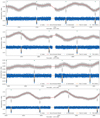 |
Fig. 2 Light curves from TESS sectors for TOI-1268 created with lightkurve from TESS tpf files. Grey points correspond to TESS observations and red lines are out-of-transit GP models created with citlalicue following the variability in LCs. This model was subtracted leading to flattened TESS LCs (blue points) with transit model (orange lines). Green triangles show the positions of transits. |
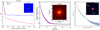 |
Fig. 3 High spatial resolution images and contrast curves for TOI-1268 used in this paper. Shown (from left to right) are the Alopeke contrast curve for 562 nm and 832 nm bands with a 1.2″ × 1.2″ reconstructed image of the field, the PHARO contrast curve for Brgamma band with a 8″ × 8″ reconstructed image of the field, and the ShaneAO contrast curve for Ks band with a 20″ × 20″ reconstructed image of the field. |
System parameters of TOI-1268.
2.4 Spectroscopic observations
2.4.1 The lull spectrograph
Between December 8, 2020, and July 18, 2021, we obtained a total of 32 spectra of TOI-1268 with the Tull spectrograph. The Tull cross-dispersed white-pupil spectrograph (Tull et al. 1995) is installed at the coudé focus of the 2.7 m Harlan J. Smith Telescope located at the McDonald Observatory. The spectrograph has a resolving power of R = 60 000 and covers wavelengths from 375 to 1020 nm. The exposure time of the observations was set to 1800 s resulting in a signal-to-noise ratio (S/N) between 60 and 75 at 550 nm, depending on the observing conditions and airmass. These spectra used an I2 vapour absorption cell as the radial velocity metric and were reduced with a pipeline script based on IRAF (Tody 1986). Radial velocities (RVs) were computed using the Austral pipeline (Endl et al. 2000).
2.4.2 The TCES spectrograph
Between March 4, 2020, and January 25, 2021, we obtained a total of 51 spectra of TOI-1268 with the Tautenburg Coudé Echelle spectrograph, attached to the 2 m Alfred Jensch telescope located at the Karl Schwarzschild Observatory. The instrument has a spectral resolving power of R = 67 000 and covers wavelengths from 467 to 740 nm. The exposure time was always set to 1800s, resulting in a typical S/N of 40 per resolution element at 550 nm depending on the observing conditions and airmass. The spectra were calibrated with an I2 vapour absorption cell and reduced with the Tautenburg Spectroscopy Pipeline–τ-spline based on IRAF and PYRAF routines (see Sabotta et al. 2019, for more details). Radial velocities were computed using the Velocity and Instrument Profile EstimatoR (VIPER2) code (Zechmeister et al. 2021).
2.4.3 The OES spectrograph
We obtained a total of 21 spectra of TOI-1268 with the spectrograph in Ondřejov between August 5, 2020, and February 24, 2021. The Ondřejov Echelle Spectrograph (OES) is installed on a 2 m Perek telescope located at the Ondřejov Observatory. The instrument has a spectral resolving power of R = 50000 (at 500 nm) and covers wavelengths from 380 to 900 nm. A detailed description of the instrument can be found in Kabáth et al. (2020). Exposure times were set to 3600 s, resulting in S/N values in the range 10–35 at 550 nm, depending on observing conditions and airmass. The spectra were calibrated with ThAr lamp spectra acquired at the end of the night and reduced with scripts based on IRAF. Radial velocities were computed with the IRAF fxcor routine.
2.4.4 The HIRES spectrograph
We obtained one spectrum of TOI-1268 with the HIRES spec-trograph (Vogt et al. 1994) on February 23, 2021. The purpose was to get a high S/N spectrum to characterise the stellar parameters. The HIRES echelle spectrograph is installed on the 10 m Keck 1 telescope and has a spectral resolving power R = 60 000 with the C2 decker. The exposure time was 90 s, resulting in an S/N of 45.
3 Stellar parameters
3.1 Stellar parameters with iSpec
We co-added all the high-resolution (R = 67 000) TCES spectra taken without iodine cells and corrected for RV shifts to reach an S/N of 45 per pixel at 550 nm. We then determined the stellar parameters of TOI-1268 by applying the Spectroscopy Made Easy radiative transfer code (SME; Valenti & Piskunov 1996; Piskunov & Valenti 2017), which is incorporated into iSpec (Blanco-Cuaresma et al. 2014; Blanco-Cuaresma 2019) on our combined spectrum. In addition, we modelled the spectrum with MARCS models of atmospheres (Gustafsson et al. 2008), which cover effective temperatures from 2500 to 8000 K, surface gravities from 0.00 to 5.00 dex, and metallicities from −5.00 to 1.00 dex. We also used version 5 of the GES atomic line list (Heiter et al. 2015). The line list spans the interval from 420 to 920 nm and includes 35 chemical species. Based on these parameters, the iSpec then calculates synthetic spectra, which are compared to the observed one, and spectral fitting technique minimises the χ2 value between them by executing a non-linear least-squares (Levenberg-Marquardt) fitting algorithm (Markwardt 2009).
To determine an effective temperature Teff, surface gravity log g, metallicity [Fe/H], and the projected stellar equatorial velocity υ sin i, we used specific features in the spectrum sensitive to these parameters. Specifically, we used the wings of the Hα line (Cayrel et al. 2011) to determine the effective temperature. We excluded the core of this line as it has its origin in the chromosphere and hence would incorrectly result in higher temperatures. We then used the 87 Fe I,II lines between 597 and 643 nm to determine a metallicity and projected stellar equatorial velocity. These parameters were used as inputs to the Bayesian parameter estimation code PARAM 1.33 (da Silva et al. 2006) to compute a surface gravity from PARSEC isochrones (Bressan et al. 2012). The whole procedure was done several times iteratively to converge to the final values of parameters. Measuring the lithium pseudo-equivalent width pEWLi of the Li I line at 670.8 nm as described in Sect. 4.4 was used as an age indicator. Finally, during the modelling process in iSpec we used empirical relations for the microturbulence and macroturbulence velocities (Vmic, Vmac) incorporated into the framework to reduce the number of free parameters. The final parameters are listed in Table 3.
The final parameters of Teff and [Fe/H] obtained after several iterations together with the Tycho V magnitude and Gaia parallax (see Table 2) were used once more as inputs to the PARAM 1.3 code to determine stellar mass, radius, and age. To estimate TOI-1268’s spectral type we used the most current version4 of the empirical spectral type-colour sequence from Pecaut & Mamajek (2013).
Stellar parameters of TOI-1268.
3.2 Stellar parameters with SpecMatch
As an independent check of the stellar parameters derived above, we also derived parameters using the HIRES spectrum and the SpecMatch package (Yee et al. 2017). To determine stellar parameters, SpecMatch compares observed spectrum with the library of well-characterised high S/N (>400) HIRES spectra in combination with Dartmouth isochrones (Dotter et al. 2008). All parameters are listed in Table 3 and are in good agreement with the values derived from iSpec. The spectrum of TOI-1268, together with the spectral synthesis fit, is plotted in Fig. 4.
3.3 SED analysis with VOSA
We modelled the spectral energy distribution (SED) using the Virtual Observatory SED Analyser (VOSA5; Bayo et al. 2008) as an additional independent check on the derived stellar parameters. We used grids of five different models: BT-Settl-AGSS2009 (Barber et al. 2006; Asplund et al. 2009; Allard et al. 2012), BT-Settl-CIFIST (Barber et al. 2006; Caffau et al. 2011; Allard et al. 2012), BT-NextGen GNS93 (Grevesse et al. 1993; Barber et al. 2006; Allard et al. 2012), BT-NextGen AGSS2009 (Barber et al. 2006; Asplund et al. 2009; Allard et al. 2012), and Coelho Synthetic stellar library (Coelho 2014) to determine effective temperature Teff, surface gravity log g, and metallicity [Fe/H]. We set priors for these parameters based on results from iSpec, specifically Teff = 4000–7000 K, log(g) = 4.0–5.0 dex, and [Fe/H] = −0.5–0.5. However, priors for metallicity are limited by model used, as for example the BT-Settl-CIFIST are available only for the solar metallicity.
We used the available photometric measurements spanning the wavelength range 0.4–22 µm (Fig. 5). Specifically, we used the Strömgren-Crawford uvbyß (Paunzen 2015), Tycho (Høg et al. 2000), Gaia DR2 (Gaia Collaboration 2018), Gaia eDR3 (Gaia Collaboration 2021), 2MASS (Cutri et al. 2003), AKARI (Ishihara et al. 2010), and WISE (Cutri et al. 2021) photometry. VOSA then uses a grid of models to compare the observed photometry with the theoretical one using χ2 minimisation procedure. For each individual model we take three results with the lowest χ2, which together create intervals of derived parameters using the lowest and highest values. We report the final intervals in Table 3. Additionally, VOSA uses the effective temperature and bolometric luminosity to determine stellar radius via the Stefan–Boltzmann law. The final intervals were derived as previously done, and are also reported in Table 3. We also used VOSA to compare TOI-1268’s SED with those in template collections provided by Kesseli et al. (2017) and to confirm the K1–K2 spectral type. All values derived from VOSA are in agreement with those inferred from iSpec and SpecMatch.
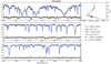 |
Fig. 4 Part of the HIRES spectrum of TOI-1268 (black) with the spectral synthesis fit (blue) and the residuals below. Also plotted are the position of TOI-1268 on the log g vs. Teff plane together with the SpecMatch library of stars with high-resolution optical spectra. |
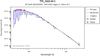 |
Fig. 5 Spectral energy distribution of TOI-1268. The red symbols represent the used photometric observations. The blue line represents the best model (BT-Settl-AGSS2009) from all different models used. The model spectrum is plotted in the background. |
3.4 Analysing stellar rotation
We used the LCs derived from the TESS target pixel files (see Sect. 2.1) to determine the rotation period of the star. Before the procedure we applied the Pixel Level Decorrelation method (Deming et al. 2015) to remove systematics. We then used the Gaussian process (GP) regression library called Celerite. A description of the library can be found in Foreman-Mackey et al. (2017a), where the authors also discuss the physical interpretation of various kernels. To derive the rotation period through the variations in LCs caused by inhomogeneous surface features, such as spots and plages, we chose a rotational kernel function defined as
![Mathematical equation: $k(\tau) = {A \over {2 + B}}{e^{- \tau /L}}\left[{\cos \left({{{2\pi \tau} \over {{P_{{\rm{rot}}}}}}} \right) + (1 + B)} \right]$](/articles/aa/full_html/2022/06/aa42883-21/aa42883-21-eq1.png) (1)
(1)
where A and B are the amplitudes of the GP, τ is the time lag, L is a timescale for the amplitude-modulation of the GP, and Prot is the rotational period. We used the L-BFGS-B nonlinear optimisation routine (Byrd et al. 1995; Zhu et al. 1997) to estimate the maximum a posteriori (MAP) parameters. We then initialised 32 walkers and run for 1000 burn-in steps and 10000steps with Markov chain Monte Carlo (MCMC) methods using emcee (Goodman & Weare 2010; Foreman-Mackey et al. 2013) to derive marginalised posterior distributions of free parameters. We used wide priors for A, B (log-uniform priors between 10−5 and 105 ppm), L (log-uniform between 10−5 and 105 days), and rotation period (uniform between 0 and 100 days). The derived rotational period from this analysis is Prot = 10.9 ± 0.5 days, and we plot the probability density of Prot together with the MAP model prediction in Fig. 6. As an independent check of the derived Prot, we also applied the generalised Lomb-Scargle (GLS) periodograms (Zechmeister & Kürster 2009) to the TESS LCs. We can see strong peaks at around 5 and 11 days in individual sectors. Using all sectors together, a forest of peaks around 11 days is visible, with the maximum at 10.9 days. We consider it to be the rotation period and its half to be the first harmonic, possibly due to spots on diametrically opposite sides of the star. We plot the periodogram in Fig. 6. This value is consistent with that inferred from the projected stellar equatorial velocity determined from the spectra. For an inclination of 90 degrees it gives a rotation period of  days. A stellar inclination close to 90 degrees would not be unexpected as, for the systems where the tidal forces are expected to play a dominant role, the tidal equilibrium can be established only under assumptions of coplanarity, circularity, and synchronised rotation (Hut 1980). Furthermore, the scenario of orbital coplanarity is highly preferred as we do not detect an additional object in the system. We report the derived rotation period in Table 3.
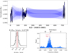 |
Fig. 6 Final plots from the stellar rotation analysis described in the paper. Top: TESS data (black points) with the MAP model prediction. The blue line shows the predictive mean, and the blue contours show the predictive standard deviation. Bottom left: probability density of the rotation period. The period is the parameter Prot in Eq. (1). The mean value is indicated by the vertical red line and the 1σ error bar is indicated by the dashed black lines. Bottom right: GLS periodogram. |
4 Age analysis
We estimated the age of TOI-1268 using several independent methods. These include stellar isochrone fitting, gyrochronology analysis, R′HK index, lithium equivalent width (EWLi), and membership to young associations. Our attempt was to examine each age indicator separately to provide the age interval for each of them and to investigate an overlap between these intervals.
4.1 Stellar isochrones
We used the PARAM 1.3 code to derive the age of TOI-1268 based on the PARSEC isochrones. As input parameters, we used the values of Teff and [Fe/H] derived in Sect. 3.1, as well as the Tycho V magnitude and the Gaia-derived parallax (see Table 2). We derived an age of 3.6 ± 3.5 Gyr. As an independent check, we overplot in Fig. 7 the TOI-1268 luminosity and effective temperature with the MIST stellar evolutionary tracks (Choi et al. 2016). It demonstrates that we are not able to distinguish between ages from about 50 Myr up to ~6 Gyr as the star is on the main sequence.
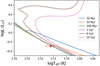 |
Fig. 7 Luminosity vs. effective temperature. The curves represent MIST isochrones for different ages: 30 Myr (blue), 50 Myr (orange), 100 Myr (green), 1 Gyr (purple), 6 Gyr (brown), 10 Gyr (pink), and for [Fe/H] = 0.25. The red point represents the parameters of TOI-1268 with their error bars. |
4.2 Gyrochronology
Gyrochronology uses the age-rotation relation to determine the ages of stars as observations of clusters reveal that rotation slows down as stars become older. Hence, we compare the rotation period versus colour of TOI-1268 with members of some well-defined clusters: M 35 (~150 Myr; Meibom et al. 2009), M 34 (~220 Myr; Meibom et al. 2011), M 37 (~400 Myr; Hartman et al. 2009), M 48 (~450 Myr; Barnes et al. 2015), Praesepe (~650 Myr; Douglas et al. 2017), NGC 6811 (~1 Gyr; Curtis et al. 2019), and NGC 6774 (~2.5 Gyr; Gruner & Barnes 2020). We used the value of TOI-1268’s rotation period measured in Sect. 3.4. In Fig. 8 we overplot TOI-1268 on the Gaia colour versus rotation period diagram with cluster members and with curves representing the gyrochronology relation from Angus et al. (2019). This empirical relation was derived from observations of rotation periods in the Praesepe cluster. According to the rotation period, TOI-1268 has an age between that of Praesepe and NGC 6811, ~650–1000 Myr.
4.3 R′HK index
We used standard relations to convert the time-averaged S-index measurements from our spectroscopy into a time-averaged measurement of the activity index, log R′HK = −4.41 ± 0. 02. According to the empirical age-activity relations of Mamajek & Hillenbrand (2008), we infer an activity age of 330 ± 50 Myr. The empirical activity-rotation relations of the same authors then predict a stellar rotation period of 9.7 ± 1.2 d for this level of activity, which is consistent with the rotation period of  days inferred from the spectroscopic υ sin i together with the stellar radius and also consistent within 1σ with the rotation period of 10.9 ± 0.5 d from the TESS LC.
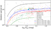 |
Fig. 8 Gaia colour vs. rotation period diagram for various members of individual clusters. The lines represent the empirical relation derived in Angus et al. (2019). TOI-1268 is indicated by a cyan star. |
4.4 Lithium equivalent width
We used the equivalent width of the lithium line as another age indicator. Lithium is known to be destroyed in the stellar interior through proton capture reactions, and the EW–age relation has been confirmed by observations of many clusters. We measured the EW of the lithium line Li 6708 Å with iSpec. To do so, we applied a procedure where the line is fitted with a Gaussian profile and the EW corresponds to the area within the Gaussian fit. We compared the EW of Li versus B–V colour to members of well-studied clusters in Fig. 9. We used the data of the Tuc-Hor young moving group (~45 Myr; Mentuch et al. 2008), the Pleiades (~120 Myr; Soderblom et al. 1993b; Lodieu et al. 2007, Lodieu et al. 2019a; Dahm 2015), M 34 (~220 Myr; Jones et al. 1997), the Ursa Major Group (~400 Myr; Soderblom et al. 1993c), Praesepe (~650 Myr; Soderblom et al. 1993a; Lodieu et al. 2019a), the Hyades (~650 Myr; Soderblom et al. 1990; Martín et al. 2018; Lodieu et al. 2018, 2019b), and M 67 (~4 Gyr; Jones et al. 1999). The data for each cluster taken from the first cited papers are plotted in Fig. 9 together with the Li EW versus B–V colour of TOI-1268 (see Table 2). According to the Li EW, TOI-1268 has an age consistent with the Pleiades and M 34. For the Pleiades we adopt the age of 110–150 Myr from the Li depletion boundary (Barrado y Navascués et al. 2004) and for the M 34 cluster, we adopt the age of 180–320 Myr based on James et al. (2010) and consistent with Jones et al. (1997). Therefore, based on the Li EW, we assign an age interval of 110–320 Myr.
4.5 Membership in young associations
We used BANYAN Σ (Gagné et al. 2018) to derive TOI-1268’s membership probability in young associations within 150 pc. BANYAN Σ is a Bayesian analysis tool that includes 27 young associations with ages in the range 1–800 Myr. In addition to BANYAN Σ, we also used the kinematic membership analysis code LocAting Constituent mEmbers In Nearby Groups (LACEwING; Riedel et al. 2017). LACEwING calculates membership probabilities in 13 young massive groups (YMGs) and three open clusters within 100 pc. All YMGs are in common with Gagné et al. (2018). As input for both codes, we used astrometric data from Gaia eDR3 listed in Table 2. Both codes reveal that TOI-1268 is a field star and is not a member of any young association. In Fig. 10 we plot the 1σ position of young stellar associations in space velocities U, V, W taken from Gagné et al. (2018) together with TOI-1268. To determine the U, V, W velocities of TOI-1268, we used the Python package PyAstronomy, specifically the gal_uvw6 function and derived U = −25.3 km s−1, V = −23.4 km s−1, and W = 10.7 km s−1. Visual inspection of the figure also did not confirm the membership in any YMGs; however, the system lies in a region typical of a young disc.
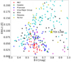 |
Fig. 9 Lithium equivalent width vs. B–V colour diagram. The points represent members of individual clusters categorised by their colours. TOI-1268 is plotted as a gold star. |
4.6 Age summary
TOI-1268 appears to be young (<1 Gyr) according to the majority of age indicators. Stellar isochrones are not very reliable because they only provide very wide estimates for main-sequence stars, and stars of TOI-1268’s age have already reached the main sequence, as predicted by stellar models (Cardona Guillén et al. 2021). Two of the activity indicators used suggest an age of the system below ~400 Myr. The only age indicator that is not consistent with this age is gyrochronology. The star appears to rotate more slowly than expected, resulting in a derived age of about 650–1000 Myr. Looking at the cluster members in Fig. 8 we can see that the expected rotation period for a star younger than ~400 Myr with the corresponding Gaia colour is below six days, hence far below the observed rotation period. We can observe some scatter for each colour and some outliers because the rotation period depends on the initial angular momentum and level of activity; however, TOI-1268’s rotation period is significantly longer than the rotation period observed in clusters of a given age.
The inconsistency between ages derived from gyrochronology and the R′HK index implies that the star either rotates too slowly for its age derived from the R′HK index, or is too active for its age derived from the rotation period. Mamajek & Hillenbrand (2008) presents the empirical relation between the R′HK index and Prot through the Rossby number Ro = Prot/τc, where τc is the convective turnover of stars. The empirical relation demonstrates that the R′HK index for solar-type dwarfs decay as the Rossby number increases. We can use this empirical relation to predict the rotation period of TOI-1268 from its level of activity. The predicted rotation period is 9.7 ± 1.2 days, which is consistent with the value derived from photometry. However, it suggests that the observed rotation period is expected for the star’s activity level. In this case, one would expect similar ages predicted from R′HK index and gyrochronology. It is not clear what causes this inconsistency. Mamajek & Hillenbrand (2008) used two different methods to derive the ages from the stellar activity for a large number of solar-type dwarfs within 16 pc. The first method directly uses the empirical relation between age and activity, and the second uses the empirical relation between activity and stellar rotation followed by gyrochronology. These ages are inconsistent for a large number of stars. Hence, in this context, inconsistent ages derived from gyrochronology and R′HK for TOI-1268 are less surprising. The equivalent width of lithium strongly favours the younger age as lithium of K-dwarf stars is expected to be depleted in Praesepe and the Hyades clusters (Soderblom et al. 1990, 1993a; Cummings et al. 2017). We adopted the more conservative age of TOI-1268 between 110 and 1000 Myr from all age indicators; however, given the majority of age indicators, we can also define a less conservative age of 110–380 Myr (see Table 4). In upcoming analyses, we either use the broad range or discuss how the results would change considering more and less conservative intervals.
Summary of age determinations of TOI-1268.
5 Analysis and results
5.1 Frequency analysis and stellar activity
In order to distinguish between the Doppler reflex motion induced by the planetary candidates and stellar activity and reveal the presence of possible additional signals, we performed a frequency analysis of the RVs and S-index activity indicator measured from the Tull spectra. All spectra used to determine the RVs of TOI-1268 were calibrated with an iodine cell, hence we can only use activity indicators uncontaminated by iodine lines. We calculated the GLS periodograms (Zechmeister & Kürster 2009) of the available time series and computed the theoretical 10, 1, and 0.1% false alarm probability (FAP) levels (Fig. 11). The baseline of our observations is about 500 days, corresponding to a frequency resolution of about 1/500 = 0.002 d−1. The most significant period is 8.2 days, which is consistent with the period of transits from TESS photometry. After fitting for this signal, we do not observe any additional significant peak in the periodogram of residuals. In the periodogram of the S-index, we do not see any significant peak. The only thing worth mentioning is the peak at 11.2 days. The fact that the peak is consistent with the star’s rotation period from photometry and is relatively isolated makes it more significant, and we interpret it as the star’s rotation period.
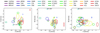 |
Fig. 10 U, V, W plots for young stellar associations and TOI-1268. The elipses represent the 1σ position of young stellar associations in space velocities U, V, W taken from Gagné et al. (2018). TOI-1268 is plotted as a magenta star. |
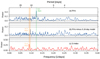 |
Fig. 11 Generalised Lomb-Scargle periodograms of RVs (blue) and S-index activity indicators (red) of TOI-1268: (a) Tull RVs, (b) Tull RVs minus 8.16-day model, (c) Tull S-index activity indicator. The vertical green line highlights the orbital period of the planet and the orange region highlights the position of stellar rotation period. The horizontal dashed lines show the theoretical FAP levels of 10, 1, and 0.1% for each panel. |
5.2 Joint RV and transit modelling
To simultaneously model transits and RVs we used the juliet package, a fitting routine described in Espinoza et al. (2019) built from several tools. The transit fitting part is based on batman (Kreidberg 2015), the radial velocity modelling part uses the package radvel (Fulton et al. 2018), and GPs modelling uses george & celerite (Ambikasaran et al. 2015; Foreman-Mackey et al. 2017b). The code performs model comparison via Bayesian evidence and explores the parameter space using nested sampling algorithms included in MultiNest (Feroz et al. 2009) via the dynesty package (Speagle 2020).
We performed a joint fit using the TESS photometry together with Tull and TCES extracted RVs. We used already corrected LCs for variability with the procedure described in Sect. 2.1. We did not include OES RVs in the final analysis as the data do not reach a precision that is sufficient to detect TOI-1268b with an average measurement error of 160 m s−1. We used them, however, as the first check to reject an eclipsing binary scenario. The juliet package uses parametrisation from Espinoza (2018). Instead of fitting for the impact parameter b and planet-to-star ratio p, it considers the parameters r1 and r2, which can be transported to the b and p through the equations found in Espinoza (2018). We also used the quadratic limb darkening law with coefficients q1 and q2. The sampling of the limb darkening coefficients follows the method described in Kipping (2013). Table 5 shows priors and posteriors of fitted parameters and Table 6 shows transit parameters and physical parameters derived from Tables 3 and 5, respectively. Phased RVs with the RV model together with phased LCs and the transit model are shown in Fig. 12. We detected a Saturn-mass planet with the RV semi-amplitude of K = 30 ± 3 m s−1 and the transit depth of δ = 8186 ± 205 ppm.
We found a slightly eccentric orbit of  . To investigate the significance of non-circular orbit, we computed the Bayesian model log evidence (ln Z) using the dynesty package to compare models with fixed zero eccentricity and eccentricity as a free parameter. If the difference in ln Z between the models is smaller than two, then they are indistinguishable (Trotta 2008). We found ∆ ln Z = 0.3, and hence, we favour a circular orbit scenario. However, we cannot rule out that the orbit is slightly eccentric.
As an independent check of derived parameters, we performed a joint fit with the pyaneti package, a PYTHON/FORTRAN fitting software described in Barragán et al. (2022) that estimates parameters of planetary systems using Markov chain Monte Carlo (MCMC) methods based on Bayesian analysis. We set uniform priors for all fitted parameters following the procedure from Barragán et al. (2016). As input stellar parameters we used those derived from the HIRES spectrum using the SpecMatch software; the stellar mass and radius derived from the parsec isochrones lead to the mean stellar density of  g cm−3, which is inconsistent with the value derived from transits described in Winn (2010). It is not clear why this is the case, and further investigation is needed. The medians and 1σ uncertainties of the fitted and derived parameters together with the stellar input parameters are listed in Table A.1. The correlations between the free parameters from the MCMC analysis and the derived posterior probability distributions are shown in Fig. A.1. All fitted parameters are in good agreement with those derived with juliet.
6 Discussion
6.1 Mass–radius diagram
By combining data from the TESS mission and ground-based spectroscopy we confirmed the planetary nature of a P = 8.16 days candidate around the V = 10.9 mag K-type star TOI-1268. We found that the physical parameters of TOI-1268b (Mp = 0.303 ± 0.026 MJ, Rp = 0.81 ± 0.05 RJ) are consistent with those of Saturn. We compared the mass and radius of TOI-1268b with the population of known planets within the mass interval 70–110 M⊕ in Fig. 13. Three subplots were created where each colour represents a different parameter: age, equilibrium temperature, and transmission spectroscopic metrics.
The most prominent group in Fig. 13 is the group of inflated planets with a radius of about 12 R⊕ or larger and equilibrium temperatures higher than 1000 K. TOI-1268b is in the second group of non-inflated planets with two members that share similar bulk properties: WASP-148b (Hébrard et al. 2020) and K2-287b (Jordán et al. 2019). The non-inflated structure of TOI-1268b is expected given its relatively low equilibrium temperature of Teq = 919K at which the inflation mechanism of hot Jupiters does not play a significant role (Kovács et al. 2010; Demory & Seager 2011). The equilibrium temperature is computed according to the equation in Kempton et al. (2018) considering zero albedo and full day-night heat redistribution. Both WASP-148b and K2-287b have equilibrium temperatures below 1000 K, a rough theoretical lower limit for planet inflation. TOI-1268b appears to be a very interesting target to explore the drivers of atmospheric inflation as it seems to be just below the threshold.
Kempton et al. (2018) proposed a metric that can be used to evaluate the suitability of planets for further atmospheric characterisation via transmission spectroscopy study. The right subplot in Fig. 13 is coloured according to this metric. We can see that TOI-1268b is one of the best candidates for the atmospheric characterisation among non-inflated Saturn-mass planets.
Fitted parameters from the juliet analysis.
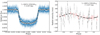 |
Fig. 12 Final plots from the joint RV and transit modelling. Left: transit LC of the TOI-1268, fitted with juliet as part of the joint analysis described in Sect. 5.2. The blue points represent TESS data together with their uncertainties, and the white points are TESS binned data. The black line represents the best transit model. Right: orbital solution for TOI-1268 showing the juliet RV model in black. The grey points represent TCES data and the red points Tull data; also shown are their uncertainties and extra jitter term plotted with the lighter grey or red, respectively. |
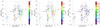 |
Fig. 13 Population of known planets within the mass interval 70–110 M⊕. The positions of TOI-1268b and two planets sharing similar properties are highlighted. The left panel is coloured with respect to the age of the systems (systems without an age estimate in the literature are in grey), the middle panel with respect to the equilibrium temperature of the planets, and the right panel with respect to the transmission spectroscopic metric. |
Derived parameters from the juliet analysis.
6.2 Tidal interaction
Giant planets, such as TOI-1268b, are thought to have formed at larger separations from their host stars and to have migrated inwards through interaction with the proto-planetary disc (Coleman et al. 2017). At close distances from the star, tidal interactions play a significant role and circularise the planetary orbit on timescales that can be calculated. There are several reasons to study tidal interactions. First, the circularisation timescales depend on the tidal quality factors of the planet and the star, which are difficult to measure. As we discuss in this section, systems such as TOI-1268 can put some constraints on these parameters. Second, if we observe an eccentric planet in an old system, where one would have expected the orbit of the planet to be already circularised, we can suspect additional interactions from another planet or a distant companion.
According to Jackson et al. (2008), the timescale for orbital circularisation for a close-in companion is
![Mathematical equation: ${1 \over {{\tau _e}}} = \left[{{{63} \over 4}\sqrt {GM_ * ^3} {{R_{\rm{p}}^5} \over {{{Q'}_{\rm{p}}}{M_{\rm{p}}}}} + {{171} \over {16}}\sqrt {G/{M_*}} {{R_*^5{M_{\rm{p}}}} \over {{{Q'}_*}}}} \right]{a^{- {{13} \over 2}}},$](/articles/aa/full_html/2022/06/aa42883-21/aa42883-21-eq23.png) (2)
(2)
where Q′* and Q′p are the tidal quality factors of the star and planet, respectively. The tidal quality factor Q is a parametrisation of the response of the body’s interior to tidal perturbation, which is defined as
 (3)
(3)
where E0 is the peak energy stored in the tidal distortion during the cycle, dE/dt is the rate of dissipation and its integral defines the energy lost during the cycle (Goldreich & Soter 1966). The tidal quality factor then represents the ratio of the elastic energy stored to the energy dissipated per cycle of the tide; larger values of tidal factors lead to longer circularisation timescales. The tidal quality factor in Eq. (2) further includes the Love number, the correction factor for the tidal-effective rigidity of the body, and its radial density distribution, Q′ = 3 Q′/2k2 (Goldreich & Soter 1966; Jackson et al. 2008). For a homogeneous fluid body k2 = 3/2. The value of Q′ is difficult to estimate, and possible values span large intervals from 102 for rocky planets (Clausen & Tilgner 2015) to 105–6 for some giant planets (Lainey et al. 2009), and up to 108–9 in the case of some stars (Collier Cameron & Jardine 2018), with typical scatter of several orders of magnitude. To assess the effect of the uncertain values of Q′* and Q′p on the circularisation timescale, in Fig. 14 we plot this timescale as a function of the tidal quality factors. We also plot the age of TOI-1268, which can be used to constrain some limits.
Before we draw any conclusions, we note that the equation above has two components. The first depends on the tidal quality factor of the planet and the second on the tidal quality factor of the star. Hence, the values of these factors, together with the planet’s mass, define which component is significant. For rocky planets with low mass and a value of Q′p ~ 102, the first component will always be dominant. For giant planets such as TOI-1268b, the first component is usually dominant, and as we see in Fig. 14 the tidal quality factor of the star starts to play a role only for Q′p > 105.5. For brown dwarfs, the second component is usually dominant, and the tidal quality factor of the planet starts to play a role only for Q′* > 106, as shown in Šubjak et al. (2020). It means that while for planets we are usually interested only in Q′p in order to study tidal interactions, for brown dwarfs, we need to consider both and Q′p, complicating the whole process. For Saturn-mass planets, it is sufficient to consider only the first component. Another important thing to note is that the circularisation timescale in this form represents the exponential damping of eccentricity on this timescale; this means that the time needed to fully circularise the orbit is two or three times greater depending on the initial value of the eccentricity. Finally, to justify the comparison of circularisation timescales with ages, we assume that the time the planet has spent at a small orbital distance is comparable with the age of the star. In other words, we assume that planets migrate inwards very early in the lifetimes of their systems (Trilling et al. 1998; Murray et al. 1998; Suárez Mascareño et al. 2021).
First, we searched for systems hosting non-inflated Saturn-mass planets on eccentric orbits to put constraints on the lower limit of Q′p. The reason why we target only non-inflated planets is that the differences in the internal structure of planets can lead to different values of Q′p. Hence, we assume that non-inflated Saturn-mass planets have a similar value of Q′p. However, this assumption is not physically justified. Examples of such systems are NGTS-11 (Gill et al. 2020) or K2-287 (Jordán et al. 2019); however, the system with ideal parameters to constrain Q′p is K2-261 (Johnson et al. 2018). K2-261 hosts a planet with Q′p mass Mp = 71 ± 10 M⊕, radius Rp = 9.5 ± 0.3 R⊕, orbital period P = 11.63344 ± 0.00012 days, and eccentricity e = 0.39 ± 0.15. Such a high eccentricity means that the age of the system is lower than the circularisation timescale (one exponential damping of eccentricity) calculated for this system, putting the lower limit on the Q′p. Furthermore, the age of the system, 8.8 ± 0.4 Gyr, is derived with great precision because the star is located near the main sequence turn-off. The derived lower limit of Q′p ~ 104.5 can be seen in Fig. 14, where we compare the circularisa-tion timescale of the system with its age. The circularisation timescale increases with increasing value of the tidal quality factor, and the position where it crosses the system’s age defines the lower limit for Q′p.
Analogously, we can discuss the upper limit of Q′p looking at systems with planets on circular orbits. Here we can use the TOI-1268 system. Even though we showed in Sect. 5.2 that the favoured eccentricity is zero, we cannot rule out that the orbit is slightly eccentric. Hence, for this system, we can only expect that the age is greater than the one circularisation timescale (i.e. one exponential damping of eccentricity; for a circular orbit, we can set the limit two or three circularisation timescales). In other words, we expect initial eccentricity after the migration to be equal to or higher than 0.15–0.35. This is supported by the observations of eccentricities in other systems, such as K2-261 or K2-287 with observed eccentricities e = 0.39 ± 0.15 and e = 0.48 ± 0.03, respectively. Furthermore, according to the Kepler survey, the systems with single transiting planets have a mean eccentricity ~0.3 (Xie et al. 2016). TOI-1268 then provide the upper limit on the value of Q′p which is Q′p ~ 104.9 as can be seen in Fig. 14. However, if we consider the broad interval for the age (see Sect. 4.6) the upper limit for Q′p would be 105.3. Hence, using lower and upper limits, we found the overlap, which is between Q′p ~ 104.5–4.9 or Q′p ~ 104.5–53 based on the age of TOI-1268. Various unknowns can affect our results, such as a gravitational interaction with other (undetected) bodies or differences in migration processes and values of initial eccentricities. Even if individual systems can be affected by these unknowns with a large sample of well-characterised Saturn-mass planets, we can obtain better insight into the general value of Q′p and test the theoretical predictions.
We can now compare these results with the tidal quality factor measured for Saturn in our Solar System. In Lainey et al. (2012) the k2/QS = 2.3 ± 0.7 × 10⁻⁴ was evaluated by studies based on the orbital migration of moons using astrometric data spanning more than a century. These values are higher than our derived interval of k2/Q = 0.2−0.5 × 10⁻⁴ (0.1−0.5 × 10⁻⁴ for the older age of TOI-1268). The recent measurements of Titan’s orbital expansion rate obtained with the Cassini spacecraft have indicated that Saturn’s Q value can be two orders of magnitude lower (k2/QS is then higher) than the value from Lainey et al. (2012). The study by Lainey et al. (2020) indicates that resonant tides are important for Saturn, and the resonance locking mechanism can explain the predicted QS based on the orbital migration of moons. Hence, comparisons with values measured for Saturn are of limited use.
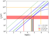 |
Fig. 14 Values of the tidal circularisation timescales as a function of planet tidal quality factor for TOI-1268b (blue lines) and K2-261 (green lines). The dashed and dotted lines of each colour represent the lower and upper boundaries of plausible values of timescales based on the parameter uncertainties used in Eq. (2). The curved blue lines represent the dependence on stellar tidal quality factors for Q′ = 104, 105, 106, 107, 108. They demonstrate that the stellar tidal quality factor influences the circularisation timescale only if the value of Q′p is larger than Q′ = 105.5. The horizontal lines show the system ages; the vertical lines give the values of Q′p in positions where timescales cross the ages of the systems. These positions define the lower limit for Q′p in the case of K2-261 and the upper limit in the case of TOI-1268. The grey region represents an overlap in Q′p between the lower limit and the upper limit. |
6.3 TOI-1268b in the context of young planets
To date, only six systems with transiting gas giant planets with measured mass are known with age below 1 Gyr: Kelt-9 (Gaudi et al. 2017), Kelt-17 (Zhou et al. 2016), WASP-178 (Rodríguez Martínez et al. 2020), Mascara-4 (Dorval et al. 2020), AU Mic (Plavchan et al. 2020; Martioli et al. 2021), and V1298 Tau (Suárez Mascareno et al. 2021; Poppenhaeger et al. 2021). There are several more systems with measured ages but without masses or only with the upper limits on their masses (Lund et al. 2017; Rizzuto et al. 2020). V1298 Tau has a young age of 10–30 Myr and AU Mic has an age of 22 ± 3 Myr, while Kelt-17 and Mascara-4 have older ages (0.5–0.9 Gyr). WASP-178 has a wide age estimate of 200–750 Myr, and Kelt-9 has an age of ~300 Myr. However, Kelt-9, together with three other systems with ages of several hundreds of years, orbits an A-type star, thereby making TOI-1268 quite distinctive and more similar to the youngest known K-dwarf star hosting giant planets, V1298 Tau (David et al. 2019).
The mass and radius of TOI-1268b are surprisingly similar to those of Saturn, hence density is similar too:  g cm−3 versus 0.69 for our Saturn, even though the system is much younger than our Solar System. We used the thermal evolution model described in Fortney et al. (2007) to determine the heavy element mass of TOI-1268b. It can be seen in Fig. 15 where we plot the isochrones in the mass-radius plane as they depend on the age of the system and the heavy element mass. The isochrones are adjusted to TOI-1268’s luminosity and TOI-1268b’s distance. We found that the heavy elements would need to have a mass of about 50 M⊕ to explain the observed mass and radius. If we consider for TOI-1268b the heavy element mass around 25 M⊕ comparable with that of Saturn, the object of TOI-1268b’s age should have a larger radius than is measured (see Fig. 15). It is consistent with the results of V1298Tau b and e (Suárez Mascareño et al. 2021) that have a mass and a radius comparable with that of Jupiter, even though the system has an age of only 10–30 Myr. Suárez Mascareño et al. (2021) suggest that current models are not able to describe well the contraction of hot giant planets, and the contraction timescale can be much shorter than expected. TOI-1268 is consistent with such a scenario. However, another process that needs to be considered is atmospheric evaporation, which is discussed in the next subsection.
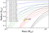 |
Fig. 15 Isochrones computed from the thermal evolution model described in Fortney et al. (2007) as they depend on the age of the system and the core’s mass. The isochrones are adjusted to TOI-1268’s luminosity and TOI-1268b’s distance. |
6.4 Atmospheric erosion
As we have shown, TOI-1268b is a Saturn-mass planet orbiting a young K dwarf, making it a potentially interesting target for the studies of atmospheric erosion. Unfortunately, the flux of the star in the X-ray and extreme UV region is unknown, so it is not yet possible to calculate the expected mass-loss rate of the planet. However, we can estimate them. Using the relation
![Mathematical equation: ${L_x}\~(3 \pm 1) \times {10^{28}}{t^{- 1.5 \pm 0.3}}[erg\,{s^{- 1}}],$](/articles/aa/full_html/2022/06/aa42883-21/aa42883-21-eq26.png) (4)
(4)
with t in Gyrs, we estimate log Lx = 28.3–30.3 (Güdel 2004). On the other hand, using the values obtained by Jackson et al. (2012) for stars in clusters of different ages, we find log Lx = 28.5–30.1. It is thus reasonable to assume that log Lx ≈ 28.5–30.0.
Together with the mass and radius obtained for the planet, this gives a mass-loss range from 1011 to 1012 gs−1 (using the same relation as in Foster et al. 2022). We used several assumptions mentioned in Foster et al. (2022) and discussed in Poppenhaeger et al. (2021). This mass loss is rather high (Foster et al. 2022). At this mass-loss rate, the planet would lose about one per cent or less of its mass in 100 Myr. Because the mass-loss rate decreases with time, it is unlikely that TOI-1268 b will become a rocky planet. However, studying a young planet with a high mass-loss rate is important to understanding the mass loss of planets in general. This is illustrated by the cases of V1298 Tau and GJ 143.
Poppenhaeger et al. (2021) studied the evaporation of the planets of the young K0–1.5 star V1298Tau in detail and concluded that the two innermost planets can lose significant fraction of their gaseous envelopes and could be evaporated down to their rocky cores, depending on the stellar spin evolution of the star. Complete erosion of the atmospheres of these planets is possible because V1298 Tau is a young active star, and the planets are small.
GJ 143 is a nearby K dwarf (Dragomir et al. 2019) of age 3.8 ± 3.7 Gyr characterised by log Lx = 27.2 (Foster et al. 2022). The outer planet GJ 143 b has a period of 35.6 days, a mass of  (Dragomir et al. 2019), and receives Fx,pl = 16 ergs−1 cm−2. Its mass-loss rate is only 5 × 10⁷g s−1 (Foster et al. 2022). The inner planet GJ 143 c has an orbital period of 7.8 days and its mass is below 3.7 M⊕ and it receives Fxpl = 123 ergs−1 cm−2. What makes this system interesting is that the inner planet is rocky, and the outer still has a gaseous envelope. It is thus possible that the inner one once also had a gaseous envelope that was eroded when the star was younger. The outer one kept its atmosphere because the erosion was not high enough to fully erode it. The very interesting aspect of this system is that the erosion must have happened when the star had an Lx-value that was in the range that we expect for TOI-1268. Studying TOI-1268 thus helps to understand the evolution of GJ143.
The examples of V1298Tau and GJ 143 show how important mass loss can be for the evolution of planets. Although we do not witness the transition from a gas giant to a rocky planet in TOI-1268, this object is an interesting case for the study of mass loss processes in young planets. TOI-1268 is a transiting planet of a nearby young star, its mass-loss rate is likely to be high, and we have determined the mass and radius of the planet. These properties make it a good target for future studies of the mass loss of planets.
Atmospheric mass loss can be constrained by measuring hydrogen and He I lines. The first detection of the evaporating atmosphere was performed by Vidal-Madjar et al. (2003) by studying the Lyman-alpha line; however, such observations are hindered by interstellar absorption and geocoronal emission. H-alpha has been detected in atmospheres of hot Jupiters around active K dwarfs (Jensen et al. 2012; Chen et al. 2020). The metastable triplet line can be used to derive mass loss, thermospheric temperature, and atmospheric dynamics through high-resolution transmission spectroscopy (Paragas et al. 2021).
TOI-1268b receives large amount of EUV radiation. We have used the relation published in Sreejith et al. (2020) to obtain log (FEUV/Fbol) = -4.48. The derived FEUV ≈ 4500 erg s−1 cm−2 suggests favourable conditions for detection of the He I and hydrogen features as the FEUV is approximately three times higher than that of WASP-69b, a planet with similar planetary parameters and strong helium features detected using the CARMENES instrument (Nortmann et al. 2018). This makes TOI-1268b an excellent candidate to study mass loss in the future.
As mentioned above, due to its high atmospheric metric TOI-1268b constitutes an excellent target for further atmospheric characterisation. The equilibrium temperature of TOI-1268b puts this planet into a class of models for equilibrium temperature of 1000 K by Fortney et al. (2010). The most prominent features in such an atmosphere are H20, Na, and K absorption. We created (Fig. 16) a simple atmospheric model in PetitRADTRANS (Mollière et al. 2019) of the expected transmission spectrum. Such atmospheric features can be detected with current instruments and make TOI-1268b a viable target for future atmospheric studies.
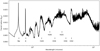 |
Fig. 16 Transit radius of the planet as a function of wavelength. The model of the transmission spectrum of TOI-1268b was generated by PetitRADTRANS (Mollière et al. 2019). The strongest atmospheric absorbers are marked. |
7 Summary
We have presented an analysis of the non-inflated Saturn-mass planet, TOI-1268b, transiting an early K-dwarf star. TOI-1268b has a moderate orbital period (P = 8.1577080 ± 0.0000044 days). The age of the system is estimated to be less than 1 Gyr using various age indicators, making the planet the youngest Saturn-mass planet known. Given a relatively bright primary, TOI-1268b is an excellent target for future transmission spectroscopy studies and one of the best from the population of non-inflated Saturn-mass planets. We have used system parameters to discuss tidal interactions and constrain the values of a tidal quality factor for non-inflated Saturn-mass planets.
TOI-1268b has also been independently confirmed by Dong et al. (2022). The two papers have been prepared and submitted simultaneously, but are the result of independent observations and analyses. We are very grateful to Jiayin Dong and collaborators for their collegiality and professionalism.
Acknowledgements
This work was supported by the KESPRINT collaboration, an international consortium devoted to the characterisation and research of exoplanets discovered with space-based missions (www.kesprint.science). J.S., R.K., M.S., M.K. and P.K. would like to acknowledge support from MSMT grant LTT-20015. J.S. and P.K. acknowledge a travel budget from ERASMUS+ grant 2020-1-CZ01-KA203-078200. J.S. would like to acknowledge support from the Grant Agency of Charles University: GAUK No. 314421. P.C. acknowledges the generous support from Deutsche Forschungsgemeinschaft (DFG) of the grant CH 2636/1-1. We are grateful for the generous support by Thüringer Ministerium für Wirtschaft, Wissenschaft und Digitale Gesellschaft. K.W.F.L. was supported by Deutsche Forschungsgemeinschaft grants RA714/14-1 within the DFG Schwerpunkt SPP 1992, Exploring the Diversity of Extrasolar Planets. N.L. was financially supported by the Ministerio de Economia y Competitividad and the Fondo Europeo de Desarrollo Regional (FEDER) under AYA2015-69350-C3-2-P. E.G. is thankful for the generously supported by the by the Thüringer Ministerium für Wirtschaft, Wissenschaft und Digitale Gesellschaft and the staff of the Alfred-Jensch-Teleskop. I.G., M.F., J.K., and C.M.P., gratefully acknowledge the support of the Swedish National Space Agency (DNR 174/18, 2020-00104, 65/19). This work was supported by JSPS KAKENHI grant number 20K14518. R.L. acknowledges financial support from the Spanish Ministerio de Ciencia e Innovación, through project PID2019-109522GB-C52, and the Centre of Excellence “Severo Ochoa” award to the Instituto de Astrofísica de Andalucía (SEV-2017-0709). L.M.S. gratefully acknowledges financial support from the CRT foundation under Grant No. 2018.2323 “Gaseous or rocky? Unveiling the nature of small worlds”. This work has been carried out within the framework of the NCCR PlanetS supported by the Swiss National Science Foundation. We acknowledge the use of public TESS data from pipelines at the TESS Science Office and at the TESS Science Processing Operations Center. Resources supporting this work were provided by the NASA High-End Computing (HEC) Program through the NASA Advanced Supercomputing (NAS) Division at Ames Research Center for the production of the SPOC data products. This paper includes data collected with the TESS mission, obtained from the MAST data archive at the Space Telescope Science Institute (STScI). Funding for the TESS mission is provided by the NASA Explorer Program. STScI is operated by the Association of Universities for Research in Astronomy, Inc., under NASA contract NAS 5-26555. This work has made use of data from the European Space Agency (ESA) mission Gaia (https://www.cosmos.esa.int/gaia), processed by the Gaia Data Processing and Analysis Consortium (DPAC, https://www.cosmos.esa.int/web/gaia/dpac/consortium). Funding for the DPAC has been provided by national institutions, in particular the institutions participating in the Gaia Multilateral Agreement. This publication makes use of VOSA, developed under the Spanish Virtual Observatory project supported by the Spanish MINECO through grant AyA2017-84089. VOSA has been partially updated by using funding from the European Union’s Horizon 2020 Research and Innovation Programme, under Grant Agreement no 776403 (EXOPLANETS-A). This research has made use of the SIMBAD database, operated at CDS, Strasbourg, France.
Appendix A Additional material
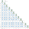 |
Fig. A.1 Correlations between the free parameters from MCMC analysis using the pyaneti code. The derived posterior probability distribution is shown at the end of each row. |
Median values and 68% confidence intervals for parameters from the pyaneti analysis
Relative radial velocities of TOI-1268 from Tautenburg and McDonald.
References
- Allard, F., Homeier, D., & Freytag, B. 2012, Phil. Trans. R. Soc. London Ser. A, 370, 2765 [Google Scholar]
- Aller, A., Lillo-Box, J., Jones, D., Miranda, L. F., & Barceló Forteza, S. 2020, A&A, 635, A128 [NASA ADS] [CrossRef] [EDP Sciences] [Google Scholar]
- Ambikasaran, S., Foreman-Mackey, D., Greengard, L., Hogg, D. W., & O’Neil, M. 2015, IEEE Trans. Pattern Anal. Mach. Intell., 38, 252 [Google Scholar]
- Angus, R., Morton, T. D., Foreman-Mackey, D., et al. 2019, AJ, 158, 173 [Google Scholar]
- Asplund, M., Grevesse, N., Sauval, A. J., & Scott, P. 2009, ARA&A, 47, 481 [NASA ADS] [CrossRef] [Google Scholar]
- Barber, R. J., Tennyson, J., Harris, G. J., & Tolchenov, R. N. 2006, MNRAS, 368, 1087 [Google Scholar]
- Barnes, S. A., Weingrill, J., Granzer, T., Spada, F., & Strassmeier, K. G. 2015, A&A, 583, A73 [NASA ADS] [CrossRef] [EDP Sciences] [Google Scholar]
- Barrado, Y. Navascués, D., Stauffer, J.R., & Jayawardhana, R. 2004, ApJ, 614, 386 [CrossRef] [Google Scholar]
- Barragán, O., Grziwa, S., Gandolfi, D., et al. 2016, AJ, 152, 193 [CrossRef] [Google Scholar]
- Barragán, O., Aigrain, S., Rajpaul, V. M., & Zicher, N. 2022, MNRAS, 509, 866 [Google Scholar]
- Bayo, A., Rodrigo, C., Barrado, Y. Navascués, D., et al. 2008, A&A, 492, 277 [NASA ADS] [CrossRef] [EDP Sciences] [Google Scholar]
- Blanco-Cuaresma, S. 2019, MNRAS, 486, 2075 [Google Scholar]
- Blanco-Cuaresma, S., Soubiran, C., Heiter, U., & Jofré, P. 2014, A&A, 569, A111 [CrossRef] [EDP Sciences] [Google Scholar]
- Bressan, A., Marigo, P., Girardi, L., et al. 2012, MNRAS, 427, 127 [NASA ADS] [CrossRef] [Google Scholar]
- Byrd, R., Lu, P., Nocedal, J., & Zhu, C. 1995, SIAM J. Sci. Comput., 16, 1190 [Google Scholar]
- Caffau, E., Ludwig, H. G., Steffen, M., Freytag, B., & Bonifacio, P. 2011, Sol. Phys., 268, 255 [Google Scholar]
- Cardona Guillén, C., Lodieu, N., Béjar, V. J. S., et al. 2021, A&A, 654, A134 [NASA ADS] [CrossRef] [EDP Sciences] [Google Scholar]
- Cayrel, R., van’t Veer-Menneret, C., Allard, N.F., & Stehlé, C. 2011, A&A, 531, A83 [NASA ADS] [CrossRef] [EDP Sciences] [Google Scholar]
- Chen, G., Casasayas-Barris, N., Pallé, E., et al. 2020, A&A, 635, A171 [NASA ADS] [CrossRef] [EDP Sciences] [Google Scholar]
- Choi, J., Dotter, A., Conroy, C., et al. 2016, ApJ, 823, 102 [Google Scholar]
- Clausen, N., & Tilgner, A. 2015, A&A, 584, A60 [NASA ADS] [CrossRef] [EDP Sciences] [Google Scholar]
- Coelho, P. R. T. 2014, MNRAS, 440, 1027 [Google Scholar]
- Coleman, G. A. L., Papaloizou, J. C. B., & Nelson, R. P. 2017, MNRAS, 470, 3206 [NASA ADS] [CrossRef] [Google Scholar]
- Collier Cameron, A., & Jardine, M. 2018, MNRAS, 476, 2542 [Google Scholar]
- Collins, K. A., Kielkopf, J. F., Stassun, K. G., & Hessman, F. V. 2017, AJ, 153, 77 [Google Scholar]
- Cummings, J. D., Deliyannis, C. P., Maderak, R. M., & Steinhauer, A. 2017, AJ, 153, 128 [Google Scholar]
- Curtis, J. L., Agüeros, M. A., Douglas, S. T., & Meibom, S. 2019, ApJ, 879, 49 [Google Scholar]
- Cutri, R. M., Skrutskie, M. F., van Dyk, S., et al. 2003, VizieR Online Data Catalog: II/246 [Google Scholar]
- Cutri, R. M., Wright, E. L., Conrow, T., et al. 2021, VizieR Online Data Catalog: II/328 [Google Scholar]
- Dahm, S. E. 2015, ApJ, 813, 108 [Google Scholar]
- da Silva, L., Girardi, L., Pasquini, L., et al. 2006, A&A, 458, 609 [NASA ADS] [CrossRef] [EDP Sciences] [Google Scholar]
- David, T. J., Petigura, E. A., Luger, R., et al. 2019, ApJ, 885, L12 [Google Scholar]
- Deming, D., Knutson, H., Kammer, J., et al. 2015, ApJ, 805, 132 [Google Scholar]
- Demory, B.-O., & Seager, S. 2011, ApJS, 197, 12 [NASA ADS] [CrossRef] [Google Scholar]
- Dong, J., Huang, C. X., Zhou, G., et al. 2022, ApJ, 926, L7 [NASA ADS] [CrossRef] [Google Scholar]
- Dorval, P., Talens, G. J. J., Otten, G. P. P. L., et al. 2020, A&A, 635, A60 [NASA ADS] [CrossRef] [EDP Sciences] [Google Scholar]
- Dotter, A., Chaboyer, B., Jevremovic, D., et al. 2008, ApJS, 178, 89 [NASA ADS] [CrossRef] [Google Scholar]
- Douglas, S. T., Agüeros, M. A., Covey, K. R., & Kraus, A. 2017, ApJ, 842, 83 [Google Scholar]
- Dragomir, D., Teske, J., Günther, M. N., et al. 2019, ApJ, 875, L7 [Google Scholar]
- Endl, M., Kürster, M., & Els, S. 2000, A&A, 362, 585 [Google Scholar]
- Espinoza, N. 2018, Res. Notes Am. Astron. Soc., 2, 209 [Google Scholar]
- Espinoza, N., Kossakowski, D., & Brahm, R. 2019, MNRAS, 490, 2262 [Google Scholar]
- Feroz, F., Hobson, M. P., & Bridges, M. 2009, MNRAS, 398, 1601 [NASA ADS] [CrossRef] [Google Scholar]
- Foreman-Mackey, D., Hogg, D. W., Lang, D., & Goodman, J. 2013, PASP, 125, 306 [Google Scholar]
- Foreman-Mackey, D., Agol, E., Ambikasaran, S., & Angus, R. 2017a, Astrophysics Source Code Library [record ascl:1709.008] [Google Scholar]
- Foreman-Mackey, D., Agol, E., Ambikasaran, S., & Angus, R. 2017b, AJ, 154, 220 [Google Scholar]
- Fortney, J. J., Marley, M. S., & Barnes, J. W. 2007, ApJ, 659, 1661 [Google Scholar]
- Fortney, J. J., Shabram, M., Showman, A. P., et al. 2010, ApJ, 709, 1396 [NASA ADS] [CrossRef] [Google Scholar]
- Fossati, L., Erkaev, N. V., Lammer, H., et al. 2017, A&A, 598, A90 [NASA ADS] [CrossRef] [EDP Sciences] [Google Scholar]
- Foster, G., Poppenhaeger, K., Ilic, N., & Schwope, A. 2022, A&A, 661, A23 [NASA ADS] [CrossRef] [EDP Sciences] [Google Scholar]
- Fridlund, M., Livingston, J., Gandolfi, D., et al. 2020, MNRAS, 498, 4503 [NASA ADS] [CrossRef] [Google Scholar]
- Fulton, B. J., Petigura, E. A., Blunt, S., & Sinukoff, E. 2018, PASP, 130, 044504 [Google Scholar]
- Gagné, J., Mamajek, E. E., Malo, L., et al. 2018, ApJ, 856, 23 [Google Scholar]
- Gaia Collaboration (Brown, A.G.A., et al.) 2018, A&A, 616, A1 [NASA ADS] [CrossRef] [EDP Sciences] [Google Scholar]
- Gaia Collaboration (Brown, A.G.A., et al.) 2021, A&A, 649, A1 [NASA ADS] [CrossRef] [EDP Sciences] [Google Scholar]
- Gaudi, B. S., Stassun, K. G., Collins, K. A., et al. 2017, Nature, 546, 514 [NASA ADS] [Google Scholar]
- Gill, S., Wheatley, P. J., Cooke, B. F., et al. 2020, ApJ, 898, L11 [Google Scholar]
- Goldreich, P., & Soter, S. 1966, Icarus, 5, 375 [Google Scholar]
- Goodman, J., & Weare, J. 2010, Commun. Appl. Math. Comput. Sci., 5, 65 [Google Scholar]
- Grevesse, N., Noels, A., & Sauval, A. J. 1993, A&A, 271, 587 [NASA ADS] [Google Scholar]
- Gruner, D., & Barnes, S. A. 2020, A&A, 644, A16 [NASA ADS] [CrossRef] [EDP Sciences] [Google Scholar]
- Güdel, M. 2004, A&ARv, 12, 71 [CrossRef] [Google Scholar]
- Guerrero, N. M., Seager, S., Huang, C. X., et al. 2021, ApJS, 254, 39 [NASA ADS] [CrossRef] [Google Scholar]
- Gustafsson, B., Edvardsson, B., Eriksson, K., et al. 2008, A&A, 486, 951 [NASA ADS] [CrossRef] [EDP Sciences] [Google Scholar]
- Hartman, J. D., Gaudi, B. S., Pinsonneault, M. H., et al. 2009, ApJ, 691, 342 [Google Scholar]
- Haswell, C. A., Fossati, L., Ayres, T., et al. 2012, ApJ, 760, 79 [Google Scholar]
- Hayward, T. L., Brandl, B., Pirger, B., et al. 2001, PASP, 113, 105 [NASA ADS] [CrossRef] [Google Scholar]
- Hébrard, G., Diaz, R. F., Correia, A. C. M., et al. 2020, A&A, 640, A32 [NASA ADS] [CrossRef] [EDP Sciences] [Google Scholar]
- Heiter, U., Lind, K., Asplund, M., et al. 2015, Phys. Scr., 90, 054010 [Google Scholar]
- Høg, E., Fabricius, C., Makarov, V. V., et al. 2000, A&A, 357, 367 [NASA ADS] [Google Scholar]
- Howell, S. B., Everett, M. E., Sherry, W., Horch, E., & Ciardi, D. R. 2011, AJ, 142, 19 [Google Scholar]
- Huang, C. X., Vanderburg, A., Pal, A., et al. 2020a, Res. Notes Am. Astron. Soc., 4, 204 [Google Scholar]
- Huang, C. X., Vanderburg, A., Pal, A., et al. 2020b, Res. Notes Am. Astron. Soc., 4, 206 [Google Scholar]
- Hut, P. 1980, A&A, 92, 167 [NASA ADS] [Google Scholar]
- Ishihara, D., Onaka, T., Kataza, H., et al. 2010, A&A, 514, A1 [NASA ADS] [CrossRef] [EDP Sciences] [Google Scholar]
- Jackson, B., Greenberg, R., & Barnes, R. 2008, ApJ, 678, 1396 [Google Scholar]
- Jackson, A. P., Davis, T. A., & Wheatley, P. J. 2012, MNRAS, 422, 2024 [Google Scholar]
- James, D. J., Barnes, S. A., Meibom, S., et al. 2010, A&A, 515, A100 [NASA ADS] [CrossRef] [EDP Sciences] [Google Scholar]
- Jenkins, J. M., Twicken, J. D., McCauliff, S., et al. 2016, SPIE Conf. Ser., 9913, 99133E [Google Scholar]
- Jensen, E. 2013, Astrophysics Source Code Library [record ascl:1306.007] [Google Scholar]
- Jensen, A. G., Redfield, S., Endl, M., et al. 2012, ApJ, 751, 86 [Google Scholar]
- Johnson, M. C., Dai, F., Justesen, A. B., et al. 2018, MNRAS, 481, 596 [NASA ADS] [CrossRef] [Google Scholar]
- Jones, B. F., Fischer, D., Shetrone, M., & Soderblom, D. R. 1997, AJ, 114, 352 [NASA ADS] [CrossRef] [Google Scholar]
- Jones, B. F., Fischer, D., & Soderblom, D. R. 1999, AJ, 117, 330 [NASA ADS] [CrossRef] [Google Scholar]
- Jordán, A., Brahm, R., Espinoza, N., et al. 2019, AJ, 157, 100 [Google Scholar]
- Kabáth, P., Skarka, M., Sabotta, S., et al. 2020, PASP, 132, 035002 [CrossRef] [Google Scholar]
- Kempton, E. M. R., Bean, J. L., Louie, D. R., et al. 2018, PASP, 130, 114401 [Google Scholar]
- Kesseli, A. Y., West, A. A., Veyette, M., et al. 2017, ApJS, 230, 16 [NASA ADS] [CrossRef] [Google Scholar]
- Kipping, D. M. 2013, MNRAS, 435, 2152 [Google Scholar]
- Kovács, G., Bakos, G. À., Hartman, J. D., et al. 2010, ApJ, 724, 866 [CrossRef] [Google Scholar]
- Kreidberg, L. 2015, PASP, 127, 1161 [Google Scholar]
- Lainey, V., Arlot, J.-E., Karatekin, Ö., & van Hoolst, T. 2009, Nature, 459, 957 [Google Scholar]
- Lainey, V., Karatekin, Ö., Desmars, J., et al. 2012, ApJ, 752, 14 [Google Scholar]
- Lainey, V., Casajus, L. G., Fuller, J., et al. 2020, Nat. Astron., 4, 1053 [Google Scholar]
- Lightkurve Collaboration (Cardoso, J.V.D.M., et al.) 2018, Astrophysics Source Code Library [record ascl:1812.013] [Google Scholar]
- Lodieu, N., Dobbie, P. D., Deacon, N. R., et al. 2007, MNRAS, 380, 712 [NASA ADS] [CrossRef] [Google Scholar]
- Lodieu, N., Rebolo, R., & Pérez-Garrido, A. 2018, A&A, 615, L12 [NASA ADS] [CrossRef] [EDP Sciences] [Google Scholar]
- Lodieu, N., Pérez-Garrido, A., Smart, R. L., & Silvotti, R. 2019a, A&A, 628, A66 [NASA ADS] [CrossRef] [EDP Sciences] [Google Scholar]
- Lodieu, N., Smart, R. L., Pérez-Garrido, A., & Silvotti, R. 2019b, A&A, 623, A35 [NASA ADS] [CrossRef] [EDP Sciences] [Google Scholar]
- Lund, M. B., Rodriguez, J. E., Zhou, G., et al. 2017, AJ, 154, 194 [Google Scholar]
- Luque, R., Serrano, L. M., Molaverdikhani, K., et al. 2021, A&A, 645, A41 [NASA ADS] [CrossRef] [EDP Sciences] [Google Scholar]
- Mamajek, E. E., & Hillenbrand, L. A. 2008, ApJ, 687, 1264 [Google Scholar]
- Markwardt, C. B. 2009, ASP Conf. Ser., 411, 251 [Google Scholar]
- Martín, E. L., Lodieu, N., Pavlenko, Y., & Béjar, V. J. S. 2018, ApJ, 856, 40 [CrossRef] [Google Scholar]
- Martioli, E., Hébrard, G., Correia, A. C. M., Laskar, J., & Lecavelier des Etangs, A. 2021, A&A, 649, A177 [NASA ADS] [CrossRef] [EDP Sciences] [Google Scholar]
- McGurk, R., Rockosi, C., Gavel, D., et al. 2014, SPIE Conf. Ser., 9148, 91483A [NASA ADS] [Google Scholar]
- Meibom, S., Mathieu, R. D., & Stassun, K. G. 2009, ApJ, 695, 679 [Google Scholar]
- Meibom, S., Barnes, S. A., Latham, D. W., et al. 2011, ApJ, 733, L9 [Google Scholar]
- Mentuch, E., Brandeker, A., van Kerkwijk, M. H., Jayawardhana, R., & Hauschildt, P. H. 2008, ApJ, 689, 1127 [NASA ADS] [CrossRef] [Google Scholar]
- Mollière, P., Wardenier, J.P., van Boekel, R., et al. 2019, A&A, 627, A67 [NASA ADS] [CrossRef] [EDP Sciences] [Google Scholar]
- Murray, N., Hansen, B., Holman, M., & Tremaine, S. 1998, Science, 279, 69 [NASA ADS] [CrossRef] [Google Scholar]
- Nortmann, L., Pallé, E., Salz, M., et al. 2018, Science, 362, 1388 [Google Scholar]
- Paragas, K., Vissapragada, S., Knutson, H. A., et al. 2021, ApJ, 909, L10 [NASA ADS] [CrossRef] [Google Scholar]
- Parviainen, H. 2015, MNRAS, 450, 3233 [Google Scholar]
- Paunzen, E. 2015, A&A, 580, A23 [NASA ADS] [CrossRef] [EDP Sciences] [Google Scholar]
- Pecaut, M. J., & Mamajek, E. E. 2013, ApJS, 208, 9 [Google Scholar]
- Perryman, M. 2018, The Exoplanet Handbook (Cambridge: Cambridge University Press) [Google Scholar]
- Persson, C. M., Csizmadia, S., Mustill, A. J., et al. 2019, A&A, 628, A64 [NASA ADS] [CrossRef] [EDP Sciences] [Google Scholar]
- Piskunov, N., & Valenti, J. A. 2017, A&A, 597, A16 [NASA ADS] [CrossRef] [EDP Sciences] [Google Scholar]
- Plavchan, P., Barclay, T., Gagné, J., et al. 2020, Nature, 582, 497 [Google Scholar]
- Pont, F. 2009, MNRAS, 396, 1789 [NASA ADS] [CrossRef] [Google Scholar]
- Poppenhaeger, K., Ketzer, L., & Mallonn, M. 2021, MNRAS, 500, 4560 [Google Scholar]
- Rasio, F. A., & Ford, E. B. 1996, Science, 274, 954 [Google Scholar]
- Riedel, A. R., Blunt, S. C., Lambrides, E. L., et al. 2017, AJ, 153, 95 [NASA ADS] [CrossRef] [Google Scholar]
- Rizzuto, A. C., Newton, E. R., Mann, A. W., et al. 2020, AJ, 160, 33 [Google Scholar]
- Rodríguez Martínez, R., Gaudi, B. S., Rodriguez, J. E., et al. 2020, AJ, 160, 111 [CrossRef] [Google Scholar]
- Sabotta, S., Kabath, P., Korth, J., et al. 2019, MNRAS, 489, 2069 [NASA ADS] [CrossRef] [Google Scholar]
- Scott, N. J., & Howell, S. B. 2018, SPIE Conf. Ser., 10701, 107010G [NASA ADS] [Google Scholar]
- Soderblom, D.R., Oey, M.S., Johnson, D.R.H., & Stone, R.P.S. 1990, AJ, 99, 595 [NASA ADS] [CrossRef] [Google Scholar]
- Soderblom, D. R., Fedele, S. B., Jones, B. F., Stauffer, J. R., & Prosser, C. F. 1993a, AJ, 106, 1080 [NASA ADS] [CrossRef] [Google Scholar]
- Soderblom, D. R., Jones, B. F., Balachandran, S., et al. 1993b, AJ, 106, 1059 [Google Scholar]
- Soderblom, D. R., Pilachowski, C. A., Fedele, S. B., & Jones, B. F. 1993c, AJ, 105, 2299 [NASA ADS] [CrossRef] [Google Scholar]
- Speagle, J. S. 2020, MNRAS, 493, 3132 [Google Scholar]
- Sreejith, A. G., Fossati, L., Youngblood, A., France, K., & Ambily, S. 2020, A&A, 644, A67 [NASA ADS] [CrossRef] [EDP Sciences] [Google Scholar]
- Staab, D., Haswell, C. A., Smith, G. D., et al. 2017, MNRAS, 466, 738 [NASA ADS] [CrossRef] [Google Scholar]
- Stassun, K. G., & Torres, G. 2021, ApJ, 907, L33 [NASA ADS] [CrossRef] [Google Scholar]
- Stassun, K. G., Oelkers, R. J., Pepper, J., et al. 2018, AJ, 156, 102 [Google Scholar]
- Suárez Mascareño, A., Damasso, M., Lodieu, N., et al. 2021, Nat. Astron., 6, 232 [Google Scholar]
- Šubjak, J., Sharma, R., Carmichael, T. W., et al. 2020, AJ, 159, 151 [Google Scholar]
- Tinetti, G., Drossart, P., Eccleston, P., et al. 2016, SPIE Conf. Ser., 9904, 99041X [NASA ADS] [Google Scholar]
- Tinetti, G., Drossart, P., Eccleston, P., et al. 2018, Exp. Astron., 46, 135 [NASA ADS] [CrossRef] [Google Scholar]
- Tody, D. 1986, SPIE Conf. Ser., 627, 733 [Google Scholar]
- Trilling, D. E., Benz, W., Guillot, T., et al. 1998, ApJ, 500, 428 [Google Scholar]
- Trotta, R. 2008, Contem. Phys., 49, 71 [NASA ADS] [CrossRef] [Google Scholar]
- Tu, L., Johnstone, C. P., Güdel, M., & Lammer, H. 2015, A&A, 577, L3 [NASA ADS] [CrossRef] [EDP Sciences] [Google Scholar]
- Tull, R. G., MacQueen, P.J., Sneden, C., & Lambert, D.L. 1995, PSAP, 107, 251 [CrossRef] [Google Scholar]
- Twicken, J. D., Catanzarite, J. H., Clarke, B. D., et al. 2018, PASP, 130, 064502 [Google Scholar]
- Valenti, J. A., & Piskunov, N. 1996, A&AS, 118, 595 [NASA ADS] [CrossRef] [EDP Sciences] [Google Scholar]
- Van Eylen, V., Astudillo-Defru, N., Bonfils, X., et al. 2021, MNRAS, 507, 2154 [NASA ADS] [Google Scholar]
- Vidal-Madjar, A., Lecavelier des Etangs, A., Désert, J.M., et al. 2003, Nature, 422, 143 [NASA ADS] [CrossRef] [Google Scholar]
- Vogt, S. S., Allen, S. L., Bigelow, B. C., et al. 1994, SPIE Conf. Ser., 2198, 362 [NASA ADS] [Google Scholar]
- Weiss, L. M., Deck, K. M., Sinukoff, E., et al. 2017, AJ, 153, 265 [NASA ADS] [CrossRef] [Google Scholar]
- Winn, J. N. 2010, in Exoplanets, ed. S. Seager (Berlin: Springer), 55 [Google Scholar]
- Wright, E. L., Eisenhardt, P.R.M., Mainzer, A.K., et al. 2010, AJ, 140, 1868 [NASA ADS] [CrossRef] [Google Scholar]
- Wuchterl, G., Guillot, T., & Lissauer, J. J. 2000, in Protostars and Planets IV, eds. V. Mannings, A.P. Boss, & S.S. Russell (Tucson: University of Arizona Press), 1081 [Google Scholar]
- Xie, J.-W., Dong, S., Zhu, Z., et al. 2016, Proc. Natl. Acad. Sci., 113, 11431 [Google Scholar]
- Yee, S. W., Petigura, E. A., & von Braun, K. 2017, ApJ, 836, 77 [Google Scholar]
- Zechmeister, M., & Kürster, M. 2009, A&A, 496, 577 [CrossRef] [EDP Sciences] [Google Scholar]
- Zechmeister, M., Köhler, J., & Chamarthi, S. 2021, Astrophysics Source Code Library [record ascl:2108.006] [Google Scholar]
- Zhou, G., Rodriguez, J. E., Collins, K. A., et al. 2016, AJ, 152, 136 [NASA ADS] [CrossRef] [Google Scholar]
- Zhu, C., Byrd, R. H., Lu, P., & Nocedal, J. 1997, ACM Trans. Math. Softw., 23, 550 [Google Scholar]
All Tables
Median values and 68% confidence intervals for parameters from the pyaneti analysis
All Figures
|
Fig. 1 Gaia DR2 catalogue overplotted to the TESS TPF image. |
| In the text | |
|
Fig. 2 Light curves from TESS sectors for TOI-1268 created with lightkurve from TESS tpf files. Grey points correspond to TESS observations and red lines are out-of-transit GP models created with citlalicue following the variability in LCs. This model was subtracted leading to flattened TESS LCs (blue points) with transit model (orange lines). Green triangles show the positions of transits. |
| In the text | |
|
Fig. 3 High spatial resolution images and contrast curves for TOI-1268 used in this paper. Shown (from left to right) are the Alopeke contrast curve for 562 nm and 832 nm bands with a 1.2″ × 1.2″ reconstructed image of the field, the PHARO contrast curve for Brgamma band with a 8″ × 8″ reconstructed image of the field, and the ShaneAO contrast curve for Ks band with a 20″ × 20″ reconstructed image of the field. |
| In the text | |
|
Fig. 4 Part of the HIRES spectrum of TOI-1268 (black) with the spectral synthesis fit (blue) and the residuals below. Also plotted are the position of TOI-1268 on the log g vs. Teff plane together with the SpecMatch library of stars with high-resolution optical spectra. |
| In the text | |
|
Fig. 5 Spectral energy distribution of TOI-1268. The red symbols represent the used photometric observations. The blue line represents the best model (BT-Settl-AGSS2009) from all different models used. The model spectrum is plotted in the background. |
| In the text | |
|
Fig. 6 Final plots from the stellar rotation analysis described in the paper. Top: TESS data (black points) with the MAP model prediction. The blue line shows the predictive mean, and the blue contours show the predictive standard deviation. Bottom left: probability density of the rotation period. The period is the parameter Prot in Eq. (1). The mean value is indicated by the vertical red line and the 1σ error bar is indicated by the dashed black lines. Bottom right: GLS periodogram. |
| In the text | |
|
Fig. 7 Luminosity vs. effective temperature. The curves represent MIST isochrones for different ages: 30 Myr (blue), 50 Myr (orange), 100 Myr (green), 1 Gyr (purple), 6 Gyr (brown), 10 Gyr (pink), and for [Fe/H] = 0.25. The red point represents the parameters of TOI-1268 with their error bars. |
| In the text | |
|
Fig. 8 Gaia colour vs. rotation period diagram for various members of individual clusters. The lines represent the empirical relation derived in Angus et al. (2019). TOI-1268 is indicated by a cyan star. |
| In the text | |
|
Fig. 9 Lithium equivalent width vs. B–V colour diagram. The points represent members of individual clusters categorised by their colours. TOI-1268 is plotted as a gold star. |
| In the text | |
|
Fig. 10 U, V, W plots for young stellar associations and TOI-1268. The elipses represent the 1σ position of young stellar associations in space velocities U, V, W taken from Gagné et al. (2018). TOI-1268 is plotted as a magenta star. |
| In the text | |
|
Fig. 11 Generalised Lomb-Scargle periodograms of RVs (blue) and S-index activity indicators (red) of TOI-1268: (a) Tull RVs, (b) Tull RVs minus 8.16-day model, (c) Tull S-index activity indicator. The vertical green line highlights the orbital period of the planet and the orange region highlights the position of stellar rotation period. The horizontal dashed lines show the theoretical FAP levels of 10, 1, and 0.1% for each panel. |
| In the text | |
|
Fig. 12 Final plots from the joint RV and transit modelling. Left: transit LC of the TOI-1268, fitted with juliet as part of the joint analysis described in Sect. 5.2. The blue points represent TESS data together with their uncertainties, and the white points are TESS binned data. The black line represents the best transit model. Right: orbital solution for TOI-1268 showing the juliet RV model in black. The grey points represent TCES data and the red points Tull data; also shown are their uncertainties and extra jitter term plotted with the lighter grey or red, respectively. |
| In the text | |
|
Fig. 13 Population of known planets within the mass interval 70–110 M⊕. The positions of TOI-1268b and two planets sharing similar properties are highlighted. The left panel is coloured with respect to the age of the systems (systems without an age estimate in the literature are in grey), the middle panel with respect to the equilibrium temperature of the planets, and the right panel with respect to the transmission spectroscopic metric. |
| In the text | |
|
Fig. 14 Values of the tidal circularisation timescales as a function of planet tidal quality factor for TOI-1268b (blue lines) and K2-261 (green lines). The dashed and dotted lines of each colour represent the lower and upper boundaries of plausible values of timescales based on the parameter uncertainties used in Eq. (2). The curved blue lines represent the dependence on stellar tidal quality factors for Q′ = 104, 105, 106, 107, 108. They demonstrate that the stellar tidal quality factor influences the circularisation timescale only if the value of Q′p is larger than Q′ = 105.5. The horizontal lines show the system ages; the vertical lines give the values of Q′p in positions where timescales cross the ages of the systems. These positions define the lower limit for Q′p in the case of K2-261 and the upper limit in the case of TOI-1268. The grey region represents an overlap in Q′p between the lower limit and the upper limit. |
| In the text | |
|
Fig. 15 Isochrones computed from the thermal evolution model described in Fortney et al. (2007) as they depend on the age of the system and the core’s mass. The isochrones are adjusted to TOI-1268’s luminosity and TOI-1268b’s distance. |
| In the text | |
|
Fig. 16 Transit radius of the planet as a function of wavelength. The model of the transmission spectrum of TOI-1268b was generated by PetitRADTRANS (Mollière et al. 2019). The strongest atmospheric absorbers are marked. |
| In the text | |
|
Fig. A.1 Correlations between the free parameters from MCMC analysis using the pyaneti code. The derived posterior probability distribution is shown at the end of each row. |
| In the text | |
Current usage metrics show cumulative count of Article Views (full-text article views including HTML views, PDF and ePub downloads, according to the available data) and Abstracts Views on Vision4Press platform.
Data correspond to usage on the plateform after 2015. The current usage metrics is available 48-96 hours after online publication and is updated daily on week days.
Initial download of the metrics may take a while.