© ESO 2022

1. Introduction

Astronomers use the emission of galaxies to determine their properties such as the stellar mass M_* and the star-formation rate SFR. However, dust within the galactic disk and star-forming regions of late-type galaxies scatters and absorbs the ultraviolet (UV), optical, and near-infrared (NIR) radiation, making the intrinsic stellar emission difficult to constrain. The absorption and scattering of light from extended objects is known as dust attenuation. Dust attenuation depends on both the dust properties (e.g., Draine & Li 2007s) and relative geometry of stars and dust (e.g., Calzetti 1997; Charlot & Fall 2000; Tuffs et al. 2004; Popescu et al. 2011) and is often mathematically indicated by an optical depth τ or a attenuation slope β. The attenuation is wavelength dependent and often expressed as follows:

$$\begin{array}{c}\hfill F_{\lambda }\approx {\lambda }^{\beta },\end{array}$$(1)

where λ is the wavelength, F_λ is the flux per wavelength, and β is the attenuation slope (Calzetti et al. 1996).

The effect of the dust distribution on attenuation can be studied using the orientation of a galaxy to the line of sight. If there were no dust, the luminosity of a galaxy would be the same for all inclinations, with only the surface brightness changing with inclination as the apparent area of the galaxy changes. However, observations show the rate at which the surface brightness increases is lower than expected because light must travel through more dust at higher galaxy inclinations (e.g., Holmberg 1958). The change in surface brightness with inclination gives us information about the dust geometry in galaxies that can help constrain the amount of dust needed to obtain dust-corrected magnitudes. Sargent et al. (2010) made use of galaxy inclination to investigate the difference in attenuation as a function of redshift. They took measurements from low-z galaxies in the Sloan Digital Sky Survey (SDSS, Abazajian et al. 2009) and galaxies at z ∼ 0.7 in the Cosmological Evolution Survey (COSMOS, Scarlata et al. 2007). They artificially redshifted the SDSS galaxies to z ∼ 0.7 and compared the surface brightness–inclination relation between the SDSS and COSMOS galaxies. They found the surface brightness–inclination relation for the COSMOS galaxies was flatter than seen for SDSS, suggesting that distant disk galaxies have a higher optical depth or a different spatial distribution of dust.

Attenuation can be modeled using radiative transfer equations that simulate interactions between photons and dust. Dust properties such as size, dust grain type, and spatial distribution relative to the stars, can be controlled in these models, allowing us to investigate their influence on attenuation. Combining the results of models with the constraints from observations allows us to study the global dust properties of galaxies.

For example, Chevallard et al. (2013) used four different models relying on different radiative transfer codes to investigate the average attenuation properties of the interstellar medium and birth clouds: Silva et al. (1998) which relies on GRAphite and SILicate (GRASIL), Tuffs et al. (2004) which relies on the code from Kylafis & Bahcall (1987), Pierini et al. (2004) which relies on DustI Radiative Transfer, Yeah! (DIRTY, Gordon et al. 2001), and Jonsson et al. (2010) which relies on SUNRISE (Jonsson 2006). Despite their differences, these models all showed similar attenuation curves at different galaxy inclinations, allowing them to be combined. Chevallard et al. (2013) applied this combined model to calculate the dust attenuation of galaxies selected from the SDSS survey following Wild et al. (2011), separating the attenuation effects of the diffuse dust and the clumpy dust based on when they would attenuate the star during stellar birth and stellar migration from the birth cloud. They found the attenuation tends to increase with the bulge-to-total ratio, while the face-on optical depth remains the same. They also found attenuation tends to change the photometry up to 0.3–0.4 mag at optical wavelengths and 0.1 mag at near-infrared wavelengths.

Given the four models compared by Chevallard et al. (2013) provided consistent results, we choose to focus on a single model in this study, the Tuffs et al. (2004) model. Several studies have obtained consistent average optical depths of large samples of low-z star-forming galaxies using only the Tuffs et al. (2004) model. Driver et al. (2007) applied the Tuffs et al. (2004) model to r-band measurements of a sample of low-z galaxies in the Millennium Galaxy Catalog to obtain the average face-on B-band optical depth ${\tau }_B^f$, finding ${\tau }_B^f=3.8_{-0.7}^{+0.7}$. Andrae et al. (2012) applied the same model on r-band measurements in low-z galaxies from the Galaxy And Mass Assembly (GAMA) survey, obtaining ${\tau }_B^f=4.0_{-0.5}^{+0.5}$.

Leslie et al. (2018a) determined attenuation using the Tuffs et al. (2004) model with FUV emission from low-z SDSS galaxies and ∼0.7 galaxies in the COSMOS field. They calculated the FUV attenuation using the expected emission from the star-formation rate main-sequence and compared the attenuation – inclination relation with the Tuffs et al. (2004) models to retrieve ${\tau }_B^f$ and the likelihood of emission being absorbed by opaque star-forming regions, given as the clumpiness F. They obtained ${\tau }_B^f=3.{95}_{-0.15}^{+0.16}$ and $F=0.{09}_{-0.02}^{+0.02}$ for the galaxies in SDSS and ${\tau }_B^f=3.5_{-1.8}^{+1.1}$ and $F=0.{55}_{-0.04}^{+0.06}$ for galaxies in COSMOS. The factor-of-five increase in the fraction of attenuation in optically thick star-forming regions (F) agrees with the increase in molecular gas mass fraction of galaxies with redshift out to z < 1. The authors concluded that the interstellar medium of galaxies is more clumpy at higher redshift. Leslie et al. (2018a) only used one UV band to constrain F, which could make the fitting sensitive to detection biases. Leslie et al. (2018b) investigated different methods of dust corrections for FUV data used to calculate SFRs for z ∼ 0 and z ∼ 0.7 galaxies. They tested three correction methods using the UV-slope β and converting β to attenuation following Boquien et al. (2012), using the attenuation – inclination relation from Tuffs et al. (2004), and using mid-infrared (MIR) hybrid corrections (Kennicutt et al. 2009; Hao et al. 2011; Catalán-Torrecilla et al. 2015). Only the UV-slope correction failed to remove the inclination dependence for z ∼ 0 galaxies. The resulting SFRs for z ∼ 0.7 galaxies using the UV-slope correction lie on average below the star-formation main-sequence (SF MS) by ∼0.44 dex. The smaller inclination dependence of FUV attenuation in the higher redshift galaxies occurs because the clumpy component F dominates the attenuation (as found by Leslie et al. 2018a). They suggested that the clumpy component and the diffuse dust disk have different UV-attenuation laws as was proposed by other studies (e.g., da Cunha et al. 2008; Wild et al. 2011; Chevallard et al. 2013).

This study expands the work done in Leslie et al. (2018a) by fitting attenuation-inclination models for multiple photometric bands and comparing the best-fit parameters at z ∼ 0 and z ∼ 0.7. We refer to the inclination using 1 − cos(i), where 1 − cos(i) = 0 is face-on, and 1 − cos(i) = 1 is edge-on. We use UV, optical, and NIR band measurements for star-forming galaxies with redshift 0.0 < z < 0.1 in the SDSS and GAMA fields and 0.6 < z < 0.8 in the COSMOS field and explain the selection process in Sect. 2. In Sect. 3, we describe the Tuffs et al. (2004) model and how we use it to retrieve the dust parameters. In Sect. 4, we show the dependence of fitted dust parameters with galaxy properties, and compare the results between low-z galaxies and galaxies at higher redshift. The properties investigated are M_*, the stellar mass surface density μ_*, SFR, the SFR per unit M_* referred to as specific star-formation rate sSFR, the distance from the star-forming main-sequence dMS, and the SFR surface density Σ_SFR. We also investigate the Hα/Hβ – inclination relation for the low-z galaxies and what set of dust parameters are required for the model to match the observations. In Sect. 5, we discuss the results, what they imply, and how they compare to previous studies of the attenuation curve. We present our conclusions in Sect. 6. For any cosmology related calculations, we assume a flat ΛCDM universe with H₀ = 70 km s⁻¹ pc, and Ω_m = 0.3.

2. Data and sample selection

We have compiled data from galaxies in two different redshift regimes: galaxies at redshift 0.04 < z < 0.1 from the SDSS and GAMA surveys, and galaxies at 0.6 < z < 0.8 from the COSMOS survey. We select galaxies at 0.04 < z < 0.1 correspond to being observed when the universe was t ∼ 13.5 Gyr old, which cover ∼5% of the age of the universe, whereas galaxies at 0.6 < z < 0.8 correspond to being observed when the universe was t ∼ 7 Gyr old, which cover ∼8%. Our selections allow us to study how dust properties have changed over ≈6.5 Gyr. The low redshift lower boundary ensures that the 3″ SDSS fiber covers at least 20% of the galaxy (Kewley et al. 2006), ensuring our Balmer line ratios used in Sect. 4.4 come from a representative region of the galaxy. We set the upper boundary (z < 0.1) to minimize galaxy evolution effects following Leslie et al. (2018a). The 0.6 < z < 0.8 redshift boundaries ensure we can retrieve similar rest-frame wavelength coverage as our low redshift sample (Kampczyk et al. 2007). We convert the photometry of all three samples to z = 0 rest-frame photometry using k-corrections. The next three subsections will cover our retrieval of literature photometric data (UV, optical, NIR, and IR), M_*, inclination, Sérsic index n, and SFR measurements. Section 2.4 explains how we select well-matched samples of star-forming galaxies.

For our study, we focus on late-type, disk-dominated galaxies for which the Tuffs et al. (2004) model was developed. Inclination and bulge-to-total ratio (B/T) are two parameters used in the Tuffs et al. (2004) model. We derive inclinations from the galaxy axis ratios and use the n as a proxy for B/T, derived from single-component Sérsic model fits on rest-frame g-band imaging across the three surveys (see Appendix B for the GAMA and COSMOS n calculations).

2.1. COSMOS

We select galaxies with redshifts 0.6 < z < 0.8 from the COSMOS Zurich Structure and Morphology Catalog (ZSMC, Scarlata et al. 2007, available on IRSA¹) in a similar manner to Sargent et al. (2010). We match the selected sample with the COSMOS2015 catalog (Laigle et al. 2016).

Photometry. The COSMOS2015 catalog contains precise PSF-matched rest-frame photometry, photometric redshifts, M_*, and SFR of more than half a million COSMOS sources. We use the measured GALEX NUV data as rest-frame GALEX FUV data because at redshift z = 0.7 the GALEX NUV band aligns with the redshift z ∼ 0.1 GALEX FUV band (Zamojski et al. 2007). For the rest-frame GALEX NUV, we use k-corrected values from the COSMOS2015 catalog, where they derived the fluxes using a spectral energy distribution (SED) that fit the detections of bands close to the NUV. We also use k-corrected photometry from the Subaru B, V, and I bands for the optical coverage and UVISTA J and K bands for the NIR coverage. We use the Spitzer Multi-band Imaging Photometer for Spitzer (MIPS) 24 μm observations (Sanders et al. 2007; Le Floc’h et al. 2009) to calculate infrared luminosities (see Sect. 3, Eq. (13)).

Properties. The COSMOS2015 photometric redshifts are calculated with the code LePHARE (Arnouts et al. 2002; Ilbert et al. 2006) using 3″ aperture fluxes and a similar method to Ilbert et al. (2013). The M_* of the galaxies is also calculated with LePHARE, creating a library of synthetic spectra generated from the stellar population synthesis model of Bruzual & Charlot (2003) assuming a Chabrier initial mass function (IMF Chabrier 2003). Throughout this study, we convert M_* and SFR to match the Kroupa IMF (Kroupa 2001) following Zahid et al. (2012). The 90% M_* completeness limit for star-forming galaxies in the redshift range of our sample (0.6 < z < 0.8) is 10⁹ M_⊙ in the UVISTA Deep field (Laigle et al. 2016). The SFR is constrained using a set of 12 templates using the Bruzual & Charlot (2003) models and optical data. For this work, we use the SFR corresponding to the maximum likelihood.

Morphology. The morphology is measured using the images from the HST Advanced Camera for Surveys (ACS) F814W I-band (Koekemoer et al. 2007) with a pixel scale of 0.05″ pixel⁻¹ and a resolution of ∼0.1″ (Scarlata et al. 2007). All galaxies in the sample with a magnitude I < 22.5 have been modeled, as described in Sargent et al. (2007), with a single component Sérsic profile using the Galaxy IMage2D package (GIM2D; Marleau & Simard 1998; Simard et al. 2002). GIM2D seeks the best-fit values for the total flux, half-light radius r_1/2, the position angle, the central position of the galaxy, the residual background level, and the ellipticity e = 1 − b/a, with a and b being the semi-major and semi-minor axes of the brightness distribution, respectively.

2.2. SDSS

We select galaxies with redshifts 0.04 < z < 0.1 from the spectroscopic catalog of SDSS Data Release 7 (DR7, Abazajian et al. 2009).

Photometry. The magnitudes of the FUV and NUV bands are provided by the GALEX Medium-depth Imaging Survey (MIS) by Bianchi et al. (2011), who matched their catalogs of unique UV sources to the seventh SDSS data release. For these GALEX bands, we find the k-correction using the IDL code kcorrect_v4_2 (Blanton & Roweis 2007) and the SDSS photometry. We draw the photometry in the optical and the near-infrared bands from the New York University (NYU) k-corrected catalog (Blanton et al. 2005). They matched the SDSS ugriz photometry to the Two Micron All Sky Survey (2MASS) JHK photometry (Skrutskie et al. 2006). Both SDSS and 2MASS photometry are used to calculate the k-corrections using kcorrect_v4_2 (Blanton et al. 2005). We add Hα and Hβ lines from the spectroscopic Max Planck for Astrophysics and Johns Hopkins University (MPA-JHU) catalog (Brinchmann et al. 2004). We use the 12 μm corrected fluxes from Chang et al. (2015) from the Wide-field Infrared Survey Explorer (WISE) survey to calculate the total infrared luminosities.

Properties. As mentioned, we use spectroscopic redshifts from the spectroscopic catalog of SDSS Data Release 7 (DR7, Abazajian et al. 2009). The total stellar masses were calculated by the MPA-JHU team from SDSS ugriz galaxy photometry using the model grids of Kauffmann et al. (2003) assuming a Kroupa IMF. We retrieve the SFR from Salim et al. (2018). They computed the SFR using Code Investigating GALaxy Emission (CIGALE; Noll et al. 2009; Boquien et al. 2019), performing SED fitting of the UV and optical photometry available in the construction of GALEX-SDSS-WISE Legacy Catalog version 1 (GSWLC-1; Salim et al. 2016). We choose these SFRs, as they align within 1σ with the SFR used in the GAMA survey.

Morphology. We add bulge+disk decomposition data from Simard et al. (2011). Simard et al. (2011) performed 2D point-spread-functions-convolved model fitting in both the g- and r-band, giving the best-fit parameters of the galaxy profile. They set the sensitivity limit of the sample to μ_1/2 = 23.0 mag arcsec⁻² for completeness and our average g-band resolution is 1.7″. For this work, we use the SDSS g-band GIM2D single Sérsic profile fits as the g-band allows for comparison with the ACS I band imaging samples at z ∼ 0.7.

2.3. GAMA

In addition to the galaxies in SDSS, we also select galaxies from the GAMA Data Release 3 (Driver et al. 2009; Baldry et al. 2018). The GAMA input catalog is based on data taken from spectroscopic SDSS and UKIRT Infrared Deep Sky Survey. GAMA is a deeper and more complete survey compared to SDSS, with an r < 19.8 magnitude limit for 98.5% redshift completeness (Baldry et al. 2018), compared to SDSS with an r < 17.7 magnitude for 94% completeness limit (Strauss et al. 2002).

Photometry. The FUV and NUV photometry is obtained from GALEX (Liske et al. 2015), the optical from VLT Survey Telescope (VST) Kilo-Degree Survey (KiDS) survey (de Jong et al. 2013), the near-infrared from Visible and Infrared Survey for Telescope for Astronomy (VISTA) Kilo-degree Infrared Galaxy (VIKING) public survey (Edge et al. 2013), and the spectra from Anglo-Australian Telescope (AAT, Liske et al. 2015). We use the updated photometric data in GALEX FUV, NUV, SDSS g, r, and i, and 2MASS J and K bands from Bellstedt et al. (2020). The k-corrections of the galaxies are calculated with kcorrect_v4_2 using magnitudes from the ApMatchedCat (Loveday et al. 2012). The Hα and Hβ fluxes are derived from Gaussian fitting following Gordon et al. (2017). We use IR data of GAMA DR3 from the WISE survey (Cluver et al. 2014) at 12 μm.

Properties. We use the spectroscopic redshifts from the GAMA survey described in Liske et al. (2015). We make use of the stellar masses in the table StellarMassLamdar, which used matched-aperture photometry from the GAMA DR 3 catalog ApMatchedCat (Hill et al. 2011; Liske et al. 2015; Driver 2015) as the input and derived the M_* using the code LAMBDAR (Wright et al. 2016). This code derives unblended photometry across the optical to NIR bands used for the fitting. Because the masses were derived with aperture photometry, we need to take into account aperture corrections using the formula:

$$\begin{array}{c}\hfill log(M_{\ast ,\mathrm{total}})=log(M_{\ast ,\mathrm{before}})+log(\mathrm{fluxscale}),\end{array}$$(2)

where M_*, before and M_*, total are the stellar mass from the LAMBDAR code before and after applying the correction respectively, and fluxscale is the documented flux ratio between the r-band flux from the LAMBDAR photometry and the Sérsic profile fitting. The fitting assumes a Chabrier IMF, which we convert to Kroupa IMF. The SFR used for the GAMA sample is calculated using MAGPHYS (da Cunha et al. 2008) adopting templates from Bruzual & Charlot (2003) and comparing SEDs to the resulting photometry of LambdarCat, taking into account the energy balance between dust absorption and dust emission. We select the SFRs found in the GaussFitSimple data table (Gordon et al. 2017).

Morphology. The half-light radii and axes ratios of the galaxies are documented in SersicCatSDSS (Kelvin et al. 2012), resulting from single Sérsic profile fits performed on the g-band images from the SDSS catalog.

2.4. Sample selection

Ideally, we would like to select samples of star-forming galaxies with similar physical properties to ensure that only the variation in dust attenuation causes differences in galaxy emission between the three catalogs. Such a selection would allow us to analyze the dust properties of galaxy populations at different redshifts. In the following, we describe our selection of star-forming galaxies (Sect. 2.4.1) and our selections on M_* and n (Sect. 2.4.2).

2.4.1. Star-formation selection

First, we classify galaxies based on their colors and use color cuts to select star-forming galaxies. We use the criteria for the NUV − r and r − J colors following Ilbert et al. (2013). For GAMA and SDSS, we also use the 3″ aperture optical spectra to select only star-forming galaxies based on their emission line ratios using the Kewley et al. (2006) diagnostic curves. We also select star-forming galaxies by their WISE photometry following the criteria from Assef et al. (2018), where the mid-IR selection identifies AGN with 90% reliability. Because we do not have the same mid-IR data for the COSMOS sample, we use a MIR-selection based on Donley et al. (2012) using SPLASH photometry to remove IR AGNs. We also remove galaxies in COSMOS with AGN based on X-ray emission (Marchesi et al. 2016):

$$\begin{array}{c}\hfill L_{\mathrm{xray}}>{10}^{42}\mathrm{erg}{\mathrm{s}}^{-1},\end{array}$$(3)

with L_xray as the 2 − 10 keV X-ray luminosity, taken from the Chandra COSMOS-Legacy survey (Civano et al. 2016; Marchesi et al. 2016).

2.4.2. Physical properties and morphology

We select galaxies within a range of physical properties. Because these physical properties are derived from photometry, we have to take into account possible detection biases. The inclination of disk galaxies impacts detection biases in two conflicting ways. More inclined galaxies will appear brighter due to their emission being spread over a smaller apparent surface area. Conversely, more inclined galaxies will also have lower apparent luminosities, especially at shorter wavelengths, due to the increase in attenuation. The combination of these effects will influence the photometry of our sample and may result in extrinsic trends between the inclination and photometry-derived galaxy properties. inclination dependent biases in physical properties in our analysis are observed in M_*, r_1/2, and n. To remove these dependencies, we calculate the median values of the physical properties for bins of inclinations and model the following relation through the data based on the method of Leslie et al. (2018a):

$$\begin{array}{c}\hfill x=a{(1-cos(i))}^b+c,\end{array}$$(4)

with x being one of the physical properties and a, b, and c are the fitting coefficients of the relations. These coefficients are given in Table 1. The results from our fitting vary slightly from Leslie et al. (2018a) as our selections differ, but the trends agree qualitatively. We find a slight positive correlation for M_* and size with inclination and a negative correlation for n.

We remove the inclination dependence found from the fitting before making cuts in physical properties by subtracting the inclination dependent part of Eq. (4) from the data. This inclination dependency of physical properties likely means there is a detection bias with inclination in the photometry. For our analysis, we compensate for the bias in photometry using a technique called importance sampling. Following Chevallard et al. (2013), we use importance sampling to weigh the galaxies based on the physical properties (z, log(M_*[M_⊙]), r_1/2, and n) and their relation with inclination. We use these weights for calculating unbiased averages of photometric data in bins of inclination to find the unbiased attenuation-inclination curve. For a more detailed explanation on importance sampling, see Appendix C.

We investigate the potential detection bias by selecting galaxies based on their S/N (S/N > 3.0) in the UV, optical, NIR, and MIR bands used for our analysis. We show these observational selections in Fig. 1. Figure 1 shows the physical property distributions of the three datasets. The properties shown are inclination 1 − cos(i), z, log(M_*), r_1/2, n and μ_*. μ_* is given by:

$$\begin{array}{c}\hfill {\mathrm{\mu }}_{\ast }=\frac{M_{\ast }}{2r_{1/2}^2}·\end{array}$$(5)

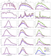Fig. 1. Distributions of the inclination corrected properties of star-forming galaxies in the three galaxy datasets SDSS, GAMA, and COSMOS, based on the different rest-frame detection criteria. The criteria are: (1) the galaxy is detected in at least one band (black), (2) the galaxy is detected in at least one UV band, one optical, one NIR, and one MIR band with S/N > 3 (blue), (3) the galaxy is detected in at least one UV band with S/N > 3 (red), (4) the galaxy is detected in at least one optical band with S/N > 3 (yellow), (5) the galaxy is detected in at least one NIR band with S/N > 3 (green), (6) the galaxy is detected in at least one MIR band with S/N > 3 (purple). The properties are, from top to bottom, inclination 1 − cos(i), redshift z, stellar mass log(M*), half-light radius r1/2, Sérsic index n and stellar mass surface density μ*. In general, the UV selection affects the number of galaxies detected in all samples. Most of the differences in selections are not visible, as the distributions overlap with each other. There is a bias toward more massive galaxies when requiring a MIR-detection in COSMOS.

The samples generally do not show a bias in a property when requiring a detection at a particular wavelength. The COSMOS sample is the only exception, where using MIR-selections would bias our sample towards higher-mass galaxies. We do not restrict our galaxies based on being detected in a specific band due to this lack of bias, resulting in a larger sample of galaxies to use for our analysis.

From the inclination corrected galaxy property distributions, we determine the cuts in physical properties needed to select disk-dominated galaxies that only differ in their redshift distribution between the three samples. We chose the cuts to ensure that the three samples are complete and have similar physical property distributions. We only select in M_* and n, with the following criteria:

$$\begin{array}{cc}\hfill 10.0& <log\left(\frac{M_{\ast }}{M_{\odot }}\right)<12.0,\hfill \\ \hfill 0.0& <n<2.5.\hfill \end{array}$$

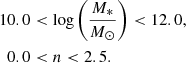
Figure 2 shows the NUV − r and r − J color–color diagram of the sample after applying the physical selections. The main purpose of this figure is to show that galaxies from the different surveys align well, especially the GAMA and COSMOS surveys.

Fig. 2. Rest-frame NUV − r and r − J color diagram of galaxies used before (gray) and after (colored) applying the selection in star-formation classification and physical properties log(M*) and n, including AGN removal. We select star-forming galaxies to lie below the black line.

We have ∼2000 galaxies for COSMOS and GAMA and ∼20 000 galaxies for SDSS after applying all the selections.

3. Methods

After applying the selections, we analyze the magnitudes of the galaxies in different bands as a function of their inclination, as shown in Fig. 3. We describe the magnitude – inclination relations using the Tuffs et al. (2004, hereafter T04) attenuation-inclination model and fit for the model parameters, making assumptions about the unattenuated emission in the GALEX UV-bands.

Fig. 3. Magnitude-inclination relations. Top row: inclination distribution of all selected star-forming galaxies in the three samples. The other panels show the magnitude-inclination relation for SDSS, GAMA, and COSMOS in rest-frame UV, optical, and NIR bands. The grayscale is a 2D histogram of all the galaxies with a signal-to-noise ratio > 3 in the respective band and the blue points show the mean values with the 32–68th percentile as errors in 10 bins of inclination using the importance sampling weights. We note that our sample selection does not require a galaxy to be detected in all photometric bands.

T04 designed a model to predict the attenuation at different UV and optical wavelengths and inclination for a star-forming galaxy with parametrised size and structures using radiative transfer modeling of UV, optical, NIR, FIR, and submm-bands multiwavelength observations of low redshift star-forming galaxies (e.g., Popescu et al. 2000). In the T04 model, a galaxy consists of two major component types: diffuse components describe the distributions of stars and dust on the scales of the galactic disks and the clumpy component describes these distributions within the star-forming regions. Specifically, the T04 model contains a dustless stellar bulge, a stellar disk harboring old stellar populations and a diffuse dust disk, a thin stellar disk harboring young stellar populations and the clumpy component, and a diffuse thin dust disk spatially correlated with the thin stellar disk. The disks and bulge were described by different exponential and de Vacouleur distributions, respectively. T04 calculated intrinsic and attenuated images of a model galaxy in eight optical and nine ultraviolet (UV) bands for the bulge, disk, and thin disk from which they derive attenuation-inclination relations. We use the updated attenuation – inclination models described in Popescu et al. (2011). The updated model uses the Weingartner & Draine (2001) and Draine & Li (2007) dust models, which include a mixture of silicate, graphite, and PAH molecules. T04 fitted the attenuation of the diffuse component in galaxies at each wavelength for different ${\tau }_B^f$ as a function of inclination with polynomial functions:

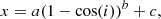
$$\begin{array}{c}\hfill \mathrm{\Delta }m\left({\tau }_B^f\right)={\mathrm{\Sigma }}_{j=0}^k{a}_j\left({\tau }_B\right){[1-cos(i)]}^j,\end{array}$$(6)

where Δm is the difference in magnitudes between the dusty images and the intrinsic images, i the inclination angle, a_j a set of coefficients for each τ_B, and k the maximum fitted power of the polynomial. T04 used k = 4 for the bulge component and k = 5 for the disk and thin disk. The ${\tau }_B^f$ used here is measured at the center of the galaxy and assumes that the dust follows an exponential profile, supported by studies of galaxies in the local Universe (e.g., Alton et al. 1998; Bianchi 2007; Muñoz-Mateos et al. 2009; Hunt et al. 2015; Casasola et al. 2017). However, when looking at our own Milky Way (Popescu et al. 2017; Natale et al. 2022) or the nearby M33 (Thirlwall et al. 2020), it was found that the dust distribution is exponential down to an inner radius, and then it decreases towards the center. So in this respect, the parameter ${\tau }_B^f$ should be thought of an effective τ, describing the global distribution of dust. The attenuation of all the components combined is given as:

$$\begin{array}{c}\hfill \begin{array}{cc}\hfill \mathrm{\Delta }{m}_{\lambda }({\tau }_B^f,i)& =2.5log(r_{\lambda }^{\mathrm{disk}}{10}^{\frac{\mathrm{\Delta }{m}_{{\lambda }^{\mathrm{disk}}}({\tau }_B^f,i)}{2.5}}\hfill \\ \hfill & +\frac{1-r_{\lambda }^{\mathrm{disk}}-r_{\lambda }^{\mathrm{bulge}}}{1-{\mathrm{Ff}}_{\lambda }}{10}^{\frac{\mathrm{\Delta }{m}_{{\lambda }^{\mathrm{tdisk}}}({\tau }_B^f,i)}{2.5}}\hfill \\ \hfill & +r_{\lambda }^{\mathrm{bulge}}{10}^{\frac{\mathrm{\Delta }{m}_{\lambda }^{\mathrm{bulge}}({\tau }_B^f,i)}{2.5}})·\hfill \end{array}\end{array}$$(7)

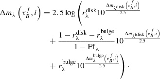
This is the general expression for the attenuation for the disk 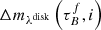$\mathrm{\Delta }{m}_{{\lambda }^{\mathrm{disk}}}({\tau }_B^f,i)$, thin disk 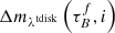$\mathrm{\Delta }{m}_{{\lambda }^{\mathrm{tdisk}}}({\tau }_B^f,i)$, and the bulge 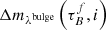$\mathrm{\Delta }{m}_{{\lambda }^{\mathrm{bulge}}}({\tau }_B^f,i)$. The attenuation per component depends on the wavelength λ, ${\tau }_B^f$, flux fractions of the bulge-to-total ratio $r_{\lambda }^{\mathrm{bulge}}$ and thin disk-to-total ratio $r_{\lambda }^{\mathrm{disk}}$, wavelength-independent clumpiness F, and wavelength-dependent conversion factor of clumpiness to attenuation f_λ, and the inclination angle i. For the clumpy component, we assume that there is no cloud fragmentation due to feedback, limiting F to be < 0.61 (see T04, Popescu et al. 2011 for more details). The wavelength dependence of f_λ only comes from the escape fraction of different types of stars. Stars with lower masses and redder emission escape further from their parent cloud in their lifetimes compared to higher mass bluer stars. Therefore, the light of redder stars is generally less attenuated by their parent clouds. In T04, they derive the wavelength-dependent values f_λ in their Appendix A, summarized in T04 Table A.1. Because the stellar components are separated based on old and young stellar population, it is possible to rewrite Eq. (7) by assuming that all UV emission comes from the young stellar disk, also refered to as the thin disk, and the optical to NIR attenuation comes from the old stellar disk, also refered to as the disk, and bulge. These assumptions mean that we can express the bulge and disk flux fractions such that:

$$\begin{array}{c}\hfill r_{\lambda }^{\mathrm{disk}}+r_{\lambda }^{\mathrm{bulge}}=1.\end{array}$$(8)

As the young stellar population dominates the UV-emission, the general expression of the T04 model is written for the UV range as:

$$\begin{array}{c}\hfill \mathrm{\Delta }{m}_{\lambda }^{\mathrm{UV}}=\mathrm{\Delta }{m}_{\lambda }^{\mathrm{tdisk}}-2.5log(1-F{f}_{\lambda }).\end{array}$$(9)

Because the old stellar population dominates the optical and NIR emission, the expressions for the optical and NIR range can be rewritten as:

$$\begin{array}{c}\hfill \mathrm{\Delta }{m}_{\lambda }^{\mathrm{optical}}=2.5log((1-r_{\lambda }^{\mathrm{bulge}}){10}^{\frac{\mathrm{\Delta }{m}_{\lambda }^{\mathrm{disk}}}{2.5}}+r_{\lambda }^{\mathrm{bulge}}{10}^{\frac{\mathrm{\Delta }{m}_{\lambda }^{\mathrm{bulge}}}{2.5}}),\end{array}$$(10)

with the attenuation of the components varying with τ_B, λ, and 1 − cos(i).

Adopting the above expressions allows us to fit for the parameters ${\tau }_B^f$, F, and hereby called bulge fraction r_bulge. Since the T04 models do not give explicit predictions for the SDSS ugriz bands, but the wavelengths corresponding to the BVIJK bands, we use interpolations to derive the attenuation values at the desired wavelengths. We separate the magnitude – inclination data into ten separate bins with an equal width in inclination or 1 − cos(i). Then, we need to derive the attenuation from our observations by normalizing the data.

Since we do not know the intrinsic emission in the optical and NIR bands, we cannot use the models directly in these bands. Instead, we normalize the data and the models by a near-face-on average magnitude, as it is the least affected by attenuation. The optical and NIR data and models are normalized to the value in the second inclination bin to avoid the low number of detections in the first bin.

However, we do need to estimate the intrinsic emission in the UV bands to fit for F describing the inclination independent offset between the attenuated and intrinsic emission. Leslie et al. (2018a) used the star-formation main-sequence and the SFR-UV conversion from Kennicutt & Evans (2012) to estimate the intrinsic UV luminosity, assuming that the sample is dominated by main-sequence galaxies. We show the results obtained using this method in Appendix E. But in this work, we aim to investigate trends as a function of galaxy parameters such as distance from the main-sequence and therefore choose to use a MIR-based correction for each galaxy. We normalize the FUV and NUV data by assuming dust-corrected FUV and NUV emission following Hao et al. (2011):

$$\begin{array}{cc}\hfill L_{\mathrm{FUV},\mathrm{corrected}}& =L_{\mathrm{FUV},\mathrm{observed}}+0.46L_{\mathrm{TIR}},\hfill \end{array}$$(11)

$$\begin{array}{cc}\hfill L_{\mathrm{NUV},\mathrm{corrected}}& =L_{\mathrm{NUV},\mathrm{observed}}+0.27L_{\mathrm{TIR}},\hfill \end{array}$$(12)

with the total infrared luminosity derived following Cluver et al. (2017):

$$\begin{array}{c}\hfill log(L_{\mathrm{TIR}})=0.889log(L_{12\mathrm{\mu }\mathrm{m}})+2.21,\end{array}$$(13)

with L_12 μm the luminosity at 12 micron in solar luminosities. For SDSS and GAMA, we use the WISE3 flux, and for COSMOS, we use the MIPS 24 μm flux and make small k-corrections using the Wuyts et al. (2008) SED template.

In these ten inclination bins, we calculate the mean magnitudes of the galaxies applying weights found using importance sampling (Appendix C). The calculated means of bins two up to nine (avoiding possible detection biases in the first and last bins affecting the results) are compared to the model value at the mean inclination per bin per waveband using the MCMC python package emcee.py (Foreman-Mackey et al. 2013) with the following likelihood function:

$$\begin{array}{c}\hfill L=-{\mathrm{\Sigma }}_k{\mathrm{\Sigma }}_i{\left(\frac{y_k\left(x_i\right)-y_{\mathrm{model},k}(x_i)}{{\sigma }_i}\right)}^2,\end{array}$$(14)

where y is the mean value in inclination bin i and band k, y_model the T04 model at mean inclination per bin x_i, and σ_i the uncertainty in the magnitude of the bands for which we use the sample standard deviation. We find the best-fit parameters by selecting the 50th percentile in the sampler distribution and the uncertainties by selecting the 32nd and 68th percentiles.

We assume uniform priors for τ_B and F over the range of the models. We limit ${\tau }_B^f$ to be between $0<{\tau }_B^f<8$, as the T04 models were calculated over this range and the model may not hold for higher values. We limit F to be between 0 < F < 0.61, as the multiplication of F with the wavelength-dependent parameter f_λ of Eq. (9) needs to be smaller than 1 to get finite numbers in a logarithm. We interpolate the wavelength-dependent parameter f_λ from T04 Table A.1 and obtain f_FUV = 1.361 for the GALEX FUV band and f_NUV = 0.839 for the GALEX NUV band. Therefore, we know that the maximum value F can have is constrained by the f_FUV, corresponding to $F=\frac{1}{1.361}=0.61$. We use the observed or inferred bulge-to-total ratio as a prior for r_bulge by fitting a skewed Gaussian distribution to the observations, assuming that the variation with optical wavelength is negligible. For SDSS, we use the B/T ratios from the g-band bulge-disk decomposition with an n = 4 bulge from Simard et al. (2011). For GAMA and COSMOS, we do not have access to B/T ratios for the full sample. Instead, we train a model using scikit learn described in Appendix B to predict the B/T using n, M_*, and color. For GAMA, we train the model using the GAMA galaxies that are also found in the SDSS sample and the g − r color, whereas for COSMOS, we use the CANDELS B/T ratios from Häußler et al. (2013) and the B − R color.

We fit all three samples separately, and by comparing SDSS and GAMA with each other, we verify whether the results for z ∼ 0.1 galaxies are robust and not dependent on the sample. The fitting is sensitive to the chosen boundaries of the priors. In Appendix D, we show how much the boundaries influence the overall results.

4. Results

We apply the fitting regime described in Sect. 3 to the selected samples from Sect. 2. First, we fit the selected data with the T04 model to study how the results for best-fit ${\tau }_B^f$, F, and r_bulge depend on redshift. Then, we investigate the fitting parameter dependence on inferred galaxy parameters, namely M_*, μ_*, SFR, sSFR, dMS, and Σ_SFR. In Sect. 4.4, we explore the dependence of the Balmer ratio Hα/Hβ on the inclination and M_* in the SDSS and GAMA samples.

4.1. T04 model fits to SDSS, GAMA, and COSMOS

We first take all the selected star-forming galaxies, compare their magnitude-inclination relations in seven bands from FUV to K, with the T04 model, and find the best-fit parameters for the SDSS, GAMA, and COSMOS data sets. The results are given in Fig. 4 and Table 2.

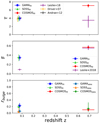Fig. 4. Results of fitting the T04 model for galaxies in the GAMA, SDSS, and COSMOS datasets. The fitted parameters are the ${\tau }_B^f$ (top), F (middle), and rbulge (bottom). We compare the fitted values of ${\tau }_B^f$ and F to the ones found in Leslie et al. (2018a), Driver et al. (2007), and Andrae et al. (2012), and the fitted values for rbulge to the average and 32–68th percentile of the bulge-to-total distribution of the selected samples, labeled with the subscript “data”. Our best-fit values are in line with the literature values. We see that ${\tau }_B^f$ and F increase with redshift.

Table 2 shows the best-fit values and their uncertainties for ${\tau }_B^f$, F and r_bulge. The fitted values for ${\tau }_B^f$ of the low redshift samples are slightly higher than what was found in Leslie et al. (2018a), Driver et al. (2007), and Andrae et al. (2012). This difference is explained by the differences between the original T04 model published in Tuffs et al. (2004), used in the reference studies, and the updated version published in Popescu et al. (2011) used for our results. Popescu et al. (2011) mention that for similar attenuation-inclination curves, the new models will have a 10% higher ${\tau }_B^f$, which explains why our results have higher ${\tau }_B^f$. The difference in F between our results and Leslie et al. (2018a) is due to the difference in methods. If we were to follow the methods described in Leslie et al. (2018a), we would obtain the same results. We investigate the effects of the assumed intrinsic UV emission in Appendix E and the number of wavelengths used in Appendix D.

Comparing our results of the 0.0 < z < 0.1 galaxies from SDSS and GAMA with the 0.6 < z < 0.8 galaxies from COSMOS shows that the ${\tau }_B^f$ and F increase with redshift, whereas the bulge fraction decreases. Our fitting results at z ∼ 0.7 are again higher than Leslie et al. (2018a), and the main difference is that they only found an increase in F with redshift but no significant increase in ${\tau }_B^f$. However, an increase in ${\tau }_B^f$ with redshift was suggested in Sargent et al. (2010), as they found a flatter B-band surface brightness – inclination relation for pure disk galaxies in COSMOS. If the surface brightness – inclination curve is flatter, it means that more light gets attenuated with inclination. Considering that Sargent et al. (2010) only looked at pure disk galaxies, we can ignore the effects of r_bulge and therefore, a steeper attenuation-inclination relation implies a higher ${\tau }_B^f$ for their sample of COSMOS galaxies at z ∼ 0.7, in qualitative agreement with our result.

In Fig. 5, we see the distribution of samplers of the MCMC fitting, illustrating how the fitted parameters are dependent on each other. We see in the figure panels that the distributions of ${\tau }_B^f$ and F are narrow for the SDSS and GAMA sample, where the 1σ value is less than 30%. The distribution of r_bulge is wider. We also see that ${\tau }_B^f$ and F are highly covariant. The COSMOS sample is best fit by values at the extreme ends of the T04 model, and as such, our uncertainties are likely underestimated.

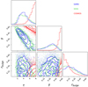Fig. 5. Results of the MCMC sampling and the best-fit parameter distributions using the T04 attenuation-inclination model. We show the fitting results for galaxies in SDSS (green), GAMA (blue), and COSMOS (red) datasets. We compare the fitted values for rbulge to the average and 32–68th percentile of the bulge-to-total distribution of the selected samples, labeled as data.

4.2. Variation of T04 model parameters with galaxy properties

After we have fitted the ${\tau }_B^f$, F, and bulge fraction of the entire sample, we now fit these parameters for different subsamples of galaxies separated by their physical properties. We aim to investigate how the magnitude-inclination relations, and thereby the T04 parameters describing global dust properties, change as a function of physical galaxy properties related to their star-formation history. We bin the galaxies in either M_*, μ_*, SFR, sSFR, dMS, or Σ_SFR, and apply the T04 model fitting in each bin to obtain the best-fit parameters for galaxy samples with varying properties. We choose the bins such that they each cover a third of the physical property range constrained from Fig. 1 after making the selection cuts. The M_* and SFR properties are sensitive to systematic differences between the samples as the M_* and SFR are derived using different SED-fitting techniques for each survey. In Fig. 6 we show that the property distributions are comparable between the three samples when making our selection cuts, which should mean that the effects of the systematic differences on our reported trends can be neglected.

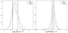Fig. 6. Distributions of our selected star-forming galaxy samples in SDSS, GAMA, and COSMOS. The figure shows the distribution in μ* (left panel), and SFR (right panel). As the COSMOS sample is selected at higher redshift, we convert the SFR to redshift z = 0 assuming that SFR ≈ (1 + z)3. Black lines show the boundaries of the bins used in our analyses.

4.2.1. Stellar mass

The first galaxy property we use for the binning is the M_*. Various studies have suggested that the M_* and the dust mass M_dust are positively correlated (e.g., Grootes et al. 2013; De Vis et al. 2017; Pastrav 2020), with the M_dust – M_* ratio depending on redshift. Because M_dust can be traced by the ${\tau }_B^f$, these results lead us to expect variations in our best-fit parameters as a function of M_*. Figure 7 and Table 3 show the best-fit parameters in three bins of M_*: 9.0 ≤ log(M_*[M_⊙]) ≤ 10.2, 10.2 ≤ log(M_*[M_⊙]) ≤ 10.5, and 10.5 ≤ log(M_*[M_⊙]) ≤ 12.0.

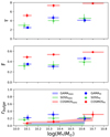Fig. 7. Best-fit values for ${\tau }_B^f$, F and rbulge for galaxies in our datasets, divided in bins of log(M*[M⊙]). We compare the fitted values for rbulge to the average and 32–68th percentile of the bulge-to-total distribution of the selected samples, labeled with the subscript “data”.

In Fig. 7 and Table 3, we see that ${\tau }_B^f$ and F increases with M_*. The fitted values for COSMOS are consistently higher compared to SDSS and GAMA, but the overall trend is the same. The increased ${\tau }_B^f$ in COSMOS relative to the low-z sample could mean that the M_dust – M_* ratio changes with redshift. Trends with r_bulge and M_* are inconsistent across the three samples and r_bulge is significantly higher than what is constrained from observations in SDSS and GAMA. However, the fitted r_bulge values are consistent within 2σ with those inferred from our Sérsic index model in the COSMOS sample. The COSMOS sample also shows a significant trend between r_bulge and M_*, with more massive galaxies being more bulge-dominated as expected (e.g., Lang et al. 2014). This could indicate that higher resolution imaging data is required to constrain accurate structural parameters; COSMOS I-band imaging probes and average of ∼0.7 kpc resolution, compared to SDSS and GAMA g band-imaging at ∼2 kpc. The lack of trend might be due to our choice of normalization by the observed magnitude value in the second inclination bin of the optical and NIR bands, where ${\tau }_B^f$ and r_bulge are the free parameters. These bands are less affected by the attenuation and, therefore, the attenuation – inclination is more shallow, which would mean that the vertical offset would have the most influence on the r_bulge and ${\tau }_B^f$. Since we cannot estimate the intrinsic emission in these bands and are only left with the inclination dependence, it would decrease the accuracy of these parameters. As the attenuation is better constrained by the inclusion of the FUV and NUV bands, where the effects are strongest and where ${\tau }_B^f$ is the only free parameter for the inclination dependent attenuation, we can still trust all our best-fit results of the τ_B. Therefore, we do not have to worry that the inconsistency in r_bulge will have a large impact on the other results.

We note that SDSS and GAMA vary slightly in the best-fit values. The reason for this effect has to do with the difference in the sample size. As our GAMA sample contains fewer galaxies than SDSS, it is more sensitive to detection bias. Our code will indicate whether the samplers of the fits converge and result in a trustworthy fit. As long as SDSS and GAMA have best-fit values within the uncertainties, we are confident in the best-fit results and trends we find for galaxies at redshift z ∼ 0.1.

4.2.2. Stellar mass surface density

Next, we divide the galaxies into bins of μ_* calculated using Eq. (5) before fitting the model. The fitting results of the three samples are given in Fig. 8 and Table 4 in bins of μ_*: 7.5 ≤ log(μ_∗[M_⊙ kpc⁻²]) ≤ 8, 8.0 ≤ log(μ_∗[M_⊙ kpc⁻²]) ≤ 8.5, and 8.5 ≤ log(μ_∗[M_⊙ kpc⁻²]) ≤ 10.0. The GAMA and COSMOS surveys do not contain enough high surface density galaxies to describe a clear magnitude-inclination relation, resulting in the model not obtaining fitting results.

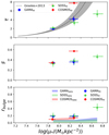Fig. 8. Best-fit values for ${\tau }_B^f$, F and rbulge for galaxies in our datasets, divided in bins of μ*. We compare the fitted values for rbulge to the average and 32–68th percentile of the bulge-to-total distribution of the selected samples, labeled with the subscript “data”. The results show an increase ${\tau }_B^f$ for an increase in μ*, similar to Grootes et al. (2013), given by the black dashed line and gray. The GAMA and COSMOS surveys do not contain enough high surface density galaxies to describe a clear magnitude-inclination relation, resulting in the model not obtaining fitting results at log(μ∗) ∼ 8.7 M⊙ kpc−2.

We see in Fig. 8 that ${\tau }_B^f$ increases when μ_* increases, with the increase being similar for SDSS and GAMA. The literature also suggests a positive τ − μ_* correlation. For example, Grootes et al. (2013) computed the ${\tau }_B^f$ of low-z galaxies based on the dust mass derived from infrared emission and fitted an empirical relation between the ${\tau }_B^f$ of the galaxies and their μ_*:

$$\begin{array}{c}\hfill log\left({\tau }_B^f\right)=1.12(\pm 0.11)·log\left(\frac{{\mathrm{\mu }}_{\ast }}{M_{\odot }{\mathrm{kpc}}^{-2}}\right)-8.6(\pm 0.8).\end{array}$$(15)

This Grootes et al. (2013) relation is shown in black in Fig. 8 and aligns with the lowest and intermediate bin for SDSS and GAMA, given the uncertainties. The highest bin for SDSS is outside of the Grootes et al. (2013) curve that suggests a ${\tau }_B^f$ beyond the model limits, implying that the T04 model cannot reproduce the attenuation-inclination relation in the highest surface density bin.

We also see that F slightly increases with the increase in μ_*, with COSMOS having the steepest increase. The increase in F for COSMOS could also be due to the model ${\tau }_B^f$ limit. The best-fit ${\tau }_B^f$ for the COSMOS sample is close to the maximum value allowed in the T04 model. If there is an increase in attenuation with μ_*, but the model is already at the maximum allowed ${\tau }_B^f$, the lack of modeled attenuation will be compensated by artificially having a higher F. We could try to extrapolate the model for ${\tau }_B^f>8$, but the current model assumptions might not hold at higher ${\tau }_B^f$. The T04 model is not calibrated for higher ${\tau }_B^f$ due to the increased likelihood of selecting starburst galaxies with irregular structures that are not expected to follow the same attenuation-inclination relation.

4.2.3. Measures of star-formation activity: SFR, sSFR, and dMS

The T04 model parameter F traces the star-forming regions of a galaxy. If the SFR or sSFR, changes, we might expect changes in these star-forming regions and, therefore, their attenuation. Figure 9 and Table 5 illustrate the best-fit model parameters in our three datasets for different bins in SFR retrieved as explained in Sect. 2. It is well known that out to redshift z≤ 2 the SFR and sSFR scales approximately with (1 + z)³ (e.g., Sargent et al. 2012; Ilbert et al. 2015; Tasca et al. 2015; Popesso et al. 2019). We scale the COSMOS SFR and sSFR by a factor of (1 + z)³ when binning in SFR and sSFR to ease comparison with the SDSS and GAMA samples. The ranges of the (scaled) SFR bins are −∞ ≤ log(SFR[M_⊙ yr⁻¹]) ≤ 0.18, 0.18 ≤ log(SFR[M_⊙ yr⁻¹]) ≤ 0.48, and 0.48 ≤ log(SFR[M_⊙ yr⁻¹]) ≤ 1. The ranges of the sSFR bins are: −15.≤log(sSFR[yr⁻¹]) ≤ −10.4, −10.4 ≤ log(sSFR [yr⁻¹]) ≤ −9.8, and −9.8 ≤ log(sSFR[yr⁻¹]) ≤ −9.0. Figure 9 and Table 5, and Fig. 10 and Table 6 show the results for SFR and sSFR respectively without the redshift-scaling.

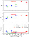Fig. 9. Best-fit values for ${\tau }_B^f$, F and rbulge for galaxies in our datasets, divided in bins of SFR. We compare the fitted values for rbulge to the average and 32–68th percentile of the bulge-to-total distribution of the selected samples, labeled with the subscript “data”. The best-fit parameters do not show a consistent correlation overall.

The best-fit results indicate that F has inconsistent trends in the three samples: it remains constant with SFR for SDSS, it slightly increases for GAMA, and it decreases for COSMOS. Figure 9 also shows that ${\tau }_B^f$ slightly increases with SFR for SDSS, but the GAMA sample does not show this trend, indicating that any trend of our best-fit parameters with SFR is not robust. The inconsistency is not a result of using different SED fitting methods to derive the SFR because the samples have similar wavelength coverage and similar assumptions where made by the different studies, each reporting a SFR averaged over the last 100 Myr. Therefore, the inconsistencies are driven by the uncertainty in the best-fit results. The trends are different when we fit in bins of sSFR; Table 6 and Fig. 10 show that there is a negative correlation between sSFR and ${\tau }_B^f$, but trends in other parameters remain unclear. The trend with ${\tau }_B^f$ and sSFR is most likely driven by the M_* because the high sSFR bin could be dominated by low-mass galaxies.

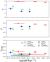Fig. 10. Best-fit values for ${\tau }_B^f$, F and rbulge for galaxies in our datasets, divided in bins of sSFR. We compare the fitted values for rbulge to the average and 32–68th percentile of the bulge-to-total distribution of the selected samples, labeled as data.

As the best-fit results still show varying trends between the samples, we investigate what might drive the observed variations by using other parameters that depend on the SFR. The first parameter we test is the star-formation main-sequence offset dMS. We define the star-formation main sequence using the relation in Leslie et al. (2018a):

$$\begin{array}{c}\hfill log\left(\frac{{\mathrm{SFR}}_{\mathrm{MS}}}{M_{\odot {\mathrm{yr}}^{-1}}}\right)=0.816log\left(\frac{M_{\ast }}{M_{\odot }}\right)-8.248+3log(1+z),\end{array}$$(16)

with SFR_MS the star-formation rate of a main-sequence galaxy, and z the corresponding redshift. The star-formation main sequence offset or the logarithmic difference between the measured SFR and the SFR derived from the star-formation main-sequence relation is given as:

$$\begin{array}{c}\hfill \mathrm{dMS}=log(\mathrm{SFR})-log\left({\mathrm{SFR}}_{\mathrm{MS}}\right).\end{array}$$(17)

Similar to our results for SFR, Fig. 11 shows no clear trends of ${\tau }_B^f$ with dMS and reveals no clear trends with F.

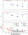Fig. 11. Best-fit values for ${\tau }_B^f$, F and rbulge for galaxies in our datasets, divided in bins of dMS. We compare the fitted values for rbulge to the average and 32–68th percentile of the bulge-to-total distribution of the selected samples, labeled as data.

However, our trends of ${\tau }_B^f$ and F with both SFR and sSFR are highly dependent on the assumed intrinsic UV emission. We discuss this further in Appendix E and the implications of the lack of correlation between F and SFR in Sect. 5.1.

4.3. Star-formation rate surface density

An important factor for star-formation is the fuel or the molecular gas. As our data do not directly measure the molecular gas, we use the star-formation rate surface density Σ_SFR as a probe for the molecular gas mass surface density (Schmidt 1959; Kennicutt 1998; Leroy et al. 2008; Bigiel et al. 2008). Table 8 and Fig. 12 show again that there is no clear correlation between Σ_SFR and any of the best-fit parameters. We note that all results showing no relation between the fitted parameters and the binned galaxy property involve the SFR. We discuss what this means in Sect. 5.1.

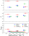Fig. 12. Best-fit values for ${\tau }_B^f$, F and rbulge for galaxies in our datasets, divided in bins of ΣSFR. We compare the fitted values for rbulge to the average and 32–68th percentile of the bulge-to-total distribution of the selected samples, labeled as data.

4.4. Balmer lines

The T04 model also allows us to describe relations between the observed Hα/Hβ ratio and the inclination of the galaxy. These ionized emission lines are assumed to come purely from our dust-enshrouded star-forming regions and also suffer attenuation from both the thin and thick disk. In the T04 model, hydrogen gas is ionized within H II regions, causing the Balmer recombination lines. Then the Balmer lines are either fully attenuated by optically thick fragments of the cloud or completely escape from the birth cloud unattenuated, similar to how the T04 model treats the attenuation of escaping stars (Sect. 3, Eq. (9)). Hβ is more likely to be scattered and absorbed by dust particles in the disk components, increasing the Hα/Hβ ratio with inclination. T04 modeled the ratio by using the radiative transfer predictions for the thin stellar disk at the wavelengths corresponding to the Hα and Hβ emission lines and fitted the ratio with a polynomial function similar to Eq. (6). In this model, the ratio is independent of F as a consequence of the assumed optical thickness and structure of the star-forming clouds. These assumptions result in the following function:

$$\begin{array}{c}\hfill \begin{array}{cc}\hfill \mathrm{H}\alpha /\mathrm{H}\beta ({\tau }_B^f,i)& =\mathrm{H}\alpha /\mathrm{H}{\beta }_{\mathrm{model}}({\tau }_B^f,i)\hfill \\ \hfill & ={\mathrm{\Sigma }}_{j=0}^k{a}_j{(1-cos(i))}^j.\hfill \end{array}\end{array}$$(18)

However, the existing T04 model could not reproduce the high ratios observed in our SDSS and GAMA samples, shown in Fig. 13. This offset could mean that there is additional dust surrounding or inside the H II region influencing the transitions on such a small spatial scale that it does not affect the UV emission (Yip et al. 2010). We use our fitting regime using the UV, optical, NIR, and Hα/Hβ data for GAMA and SDSS and add a parameter C, describing the offset in the Hα/Hβ-inclination relation compared to the model:

$$\begin{array}{c}\hfill \mathrm{H}\alpha /\mathrm{H}\beta ({\tau }_B^f,i)={\mathrm{\Sigma }}_{j=0}^k{a}_j{(1-cos(i))}^j+C.\end{array}$$(19)

Fig. 13. Hα/Hβ ratio for the SDSS and GAMA sample for galaxies with varying inclination. Top two panels: inclination distribution, and the bottom two panels show the Hα/Hβ – inclination relation for the selected star-forming sample and the Hα/Hβ ratio – inclination relation from the T04 model with varying ${\tau }_B^f$. We can see that none of the T04 models can describe the observed trend.

After investigating the fitting of C and how it varies with galaxy properties, we found consistent inter-sample trends for ${\tau }_B^f$, F, and C with variation in M_*. We show the results in Table 9 and Fig. 14.

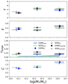Fig. 14. Best-fit values for ${\tau }_B^f$, F, rbulge, and C for galaxies in our datasets, divided in bins of mass log(M*[M⊙]).

In our new model shown in Table 9 and Fig. 14, we see similar trends with Table 3 and Fig. 7. The ${\tau }_B^f$ increases over bins of M_*, whereas the F remains constant. Our results for ${\tau }_B^f$, F, and r_bulge are consistent with what we found in Sect. 4.2.1, meaning the addition of the Hα/Hβ ratio provides no additional constraints. We find that C increases with the M_* of the galaxy. This result means that the star-forming regions have a component not described in the T04 models, with a wavelength-dependent attenuation influencing the Balmer ratio. This component varies with the global stellar masses.

5. Discussion

With the fitting of the T04 parameters in bins of different galaxy properties, we now discuss the results of Sect. 4.2 to gain insight into how the dust and galaxy properties are linked. In this section, we discuss the correlations found in more detail and describe their implications for dust formation and how different tracers could influence these implications.

5.1. Dependence of model parameters on galaxy properties

We find an increase in ${\tau }_B^f$ with an increase in M_* and μ_*. Popescu et al. (2011) shows that ${\tau }_B^f$ can be linked to M_dust based on the scale length of the stellar disk, the geometry of the dust, and dust properties (see Popescu et al. 2011 Sect. 2.9, Eq. (44) for more information). Therefore, our results could imply that galaxies with higher M_* have higher M_dust (e.g., Liu et al. 2019; Magnelli et al. 2020; Kokorev et al. 2021) hinting at the paired production of stars and dust (e.g., De Vis et al. 2017; Pastrav 2020). The correlation with μ_* is similar to the Grootes et al. (2013) relation for low-z galaxies but deviates for high-μ_* galaxies and high-z because the T04 model is unable to cover the high τ_B estimated by the Grootes et al. (2013) relation for these bins. The variation of M_dust with galaxy properties is often traced using the ratio of the dust mass with the stellar mass M_dust/M_*. Studies report an anticorrelation between M_dust/M_* with the M_* both in the local universe (e.g., Cortese et al. 2012; Clemens et al. 2013; Orellana et al. 2017; Casasola et al. 2020), and out to z ∼ 2 (e.g., Calura et al. 2017) with a slope ranging from −1 to 0, supporting our inferred positive relation between M_dust and M_*.

da Cunha et al. (2010) investigated the relation between M_dust of a galaxy and the SFR using the model of da Cunha et al. (2008). They used the two-screen attenuation relation from Charlot & Fall (2000) and separate attenuation from the interstellar medium and the birth clouds to calculate SED templates that best fit the observed galaxies in SDSS DR6. da Cunha et al. (2010) reported an increase in M_dust with SFR for SDSS galaxies with −2.0 < log(SFR/M_⊙ yr⁻¹)) < 2.0. Although we find a positive correlation between ${\tau }_B^f$ (related to M_dust) and SFR in the SDSS sample, we did not see this trend in the GAMA or COSMOS samples. Similarly, the three samples show inconsistent trends for F and r_bulge with SFR. Our investigation of dMS and Σ_SFR also resulted in inconsistent trends for all three samples.

Our interpretation that the ${\tau }_B^f$, and therefore M_dust, is independent of SFR is supported by the literature. For example, Casasola et al. (2017) investigated the radial distribution of the dust, gas, stars, and SFR using data from DustPedia (Davies et al. 2017). They found that the scale length for the dust-mass surface-density distribution is 1.8 times higher than for the SFR, assuming that both properties follow an exponential distribution. This is a consequence of the fact that the scale length of the stellar emissivity of the young stellar population is usually smaller than the scale length of the dust, a result derived from radiative transfer models of well-resolved galaxies (e.g., Xilouris et al. 1999; Popescu et al. 2000, 2017; Misiriotis et al. 2001; Thirlwall et al. 2020; Natale et al. 2022). The difference in scale-length indicates that M_dust and SFR are not always spatially correlated, implying that the dust mass is not fully correlated with the SFR. The independence of ${\tau }_B^f$ on the SFR could be due to a negative feedback mechanism, for example, radiative feedback, that regulates dust formation.

Casasola et al. (2017) also found that the dust-mass surface-density distribution differs from the stellar-mass surface-density distribution, which would imply that M_dust and M_* are not spatially correlated. This is again a consequence of the fact that the scale-length of the dust distribution is usually larger than the scale length of the NIR emissivity of the older stellar population that makes the bulk of the M_*, result also found in radiative transfer models of individual well-resolved galaxies (e.g., Xilouris et al. 1999; Popescu et al. 2000, 2017; Misiriotis et al. 2001; Thirlwall et al. 2020; Natale et al. 2022). Other spatially resolved studies, such as Smith et al. (2016), have found a spatial correlation between M_dust and the M_* up to twice the optical radius r₂₅. Whether or not M_dust and M_* are spatially correlated is still debated as the analysis of global properties indicate that there is a link between the M_dust and the M_* (e.g., Cortese et al. 2012; Clemens et al. 2013; Orellana et al. 2017; Calura et al. 2017; Casasola et al. 2020). Considering the inconsistent trends with SFR, we interpret the anticorrelation found between ${\tau }_B^f$ and sSFR to be driven by the M_* rather than the star-formation timescale.

The SFR surface density Σ_SFR can be used as a tracer for the total gas mass surface density following seminal work by Kennicutt (1998). Several studies have shown that the dust and total gas are correlated (e.g., Corbelli et al. 2012; Sandstrom et al. 2013; Groves et al. 2015; Casasola et al. 2020), with the correlation dependent on the metallicity and the heating effects within a galaxy (e.g., Lisenfeld & Ferrara 1998; Draine et al. 2007; Galliano et al. 2008; Rémy-Ruyer et al. 2014; De Vis et al. 2017). Constraining the amount of total gas from Σ_SFR is non trivial. Many studies of the Schmidt–Kennicutt relation have been performed on both galactic and subgalactic scales and find different results for the slope of the relation due to, for example, methodology, tracers used, sample selection, and influence of other galaxy properties such as Σ_* (Bigiel et al. 2008; Casasola et al. 2015; Ellison et al. 2020; Morselli et al. 2020; Kennicutt & De Los Reyes 2021). However, it is now well established that Σ_SFR is more closely correlated with the molecular gas mass surface density than total gas surface density (e.g., Leroy et al. 2008; Schruba et al. 2011). Although there are hints of a positive correlation between the dust mass and the molecular gas mass, this relationship comes with considerable scatter (e.g., Orellana et al. 2017; Casasola et al. 2020). Furthermore, the correlation between dust mass and ${\tau }_B^f$ is dependent on the scale height and relative distribution of stars and dust (Popescu et al. 2011), bringing uncertainties in relating our inferred ${\tau }_B^f$ with dust mass. Given the systematic differences in Schmidt–Kennicutt relations, combined with the complex relationships between atomic gas, molecular gas, dust, and SFR, it is not surprising that we find inconsistent trends between Σ_SFR and ${\tau }_B^f$ for our three samples. Future work could verify our results by using a more direct tracer of molecular gas mass, such as CO luminosity or dust emission in the Rayleigh–Jeans tail of the SED (e.g., Corbelli et al. 2012; Casasola et al. 2020).

In Appendix E, we show the results of Sect. 4.1 assuming different star-formation rate main-sequence relations and applying the Kennicutt & Evans (2012) SFR-luminosity conversion to estimate the intrinsic emission in FUV and NUV. We find no trends of F with SFR when adopting different main-sequence normalizations. On the other hand, we find that any relations between F and M_* or μ_* vary depending on the main-sequence adopted. A possible explanation for this variation could be that the derived star-formation main-sequences are themselves affected by attenuation biases. The UV-SFR calibration from Kennicutt & Evans (2012) assumes a constant star-formation history over the past 100 Myr, however galaxies above and below the main sequence have been shown to have rising and falling star-formation histories, respectively (e.g., Leja et al. 2019), rendering the UV calibration inaccurate in particular bins. An incorrect SFR calibration would cause a bias in our corrected FUV and NUV magnitudes, resulting in biased best-fitted values for F. Therefore, we chose not to use them to estimate intrinsic emissions. A different study would also be to check whether we need more accurate dust attenuation corrections than those derived from MIR. We found that a change in the star-formation main-sequence adopted does not influence the relative relations between ${\tau }_B^f$ and M_* or μ_*, which is further evidence that the M_* is strongly linked to the dust mass.

5.2. Evolution of dust properties

Figure 15 summarizes how our model parameters ${\tau }_B^f$ and F, as well as galaxy molecular to stellar mass ratio (M_H2/M_*), specific SFR, SFR efficiency (SFR/M_H2), and metallicity (log(O/H)+12) increase relative to their values at z = 0.07. For our z = 0.07 reference, we have averaged the SDSS and GAMA values for ${\tau }_B^f$ and F because they are consistent within the errors. We find that values of ${\tau }_B^f$ and F are both a factor ∼1.75 higher in the COSMOS sample, implying these dust parameters scale roughly with (1 + z). Galaxy star-formation efficiency (inverse of depletion time), calculated for galaxies between 10.2 < log(M_*[M_⊙]) < 11.5 (the M_* range of our samples), increases by a similar amount, according to the scaling relations reported by Liu et al. (2019, see Fig. 15).

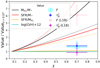Fig. 15. Evolution of massive galaxy properties from their low-z values out to z ∼ 1. Relationships for molecular gas to stellar mass ratio (MH2/M*), specific SFR, SFR efficiency (SFR/MH2), and metallicity (log(O/H)+12) are from the A3COSMOS scaling relations for main-sequence galaxies derived by Liu et al. (2019), adopting the Schreiber et al. (2015) main-sequence. Solid lines show the relations at log(M*/M⊙) = 10.2 and dotted lines show the relations for galaxies with log(M*/M⊙) = 11.5. Unlike (Leslie et al. 2018a, L18), who found that F increases with redshift and the τB ${\tau }_B^f$ remains constant to z ∼ 0.7, we find that both these dust parameters evolve together increasing by a factor of ∼1.7 (${\tau }_B^f$) and ∼1.8 (F) from low-z galaxies in GAMA and SDSS to intermediate-redshift galaxies in COSMOS.

The ${\tau }_B^f$ for z ∼ 0.7 galaxies in COSMOS is higher than that found for z ∼ 0 galaxies in SDSS and GAMA at fixed M_*, implying different relations between M_dust and the M_* for galaxies at different redshifts (e.g., Béthermin et al. 2015; De Vis et al. 2017; Calura et al. 2017; Pastrav 2020). Béthermin et al. (2015) studied the mean M_dust – M_* ratio for star-forming galaxies with M_∗ > 3 × 10¹⁰ M_⊙ across redshift. They found that the M_dust – M_* ratio increased with redshift M_dust/M_* ≈ (1 + z)^x with x > 0.05 (Tan et al. 2014) up to a redshift of z = 1 for star-formation main-sequence galaxies, whereafter it became constant. Because the COSMOS sample has higher fitted ${\tau }_B^f$, indicating a higher average M_dust, compared to SDSS and GAMA at similar M_*, our results imply a correlation between the M_dust – M_* ratio and redshift, which is consistent with the literature (e.g., Liu et al. 2019; Magnelli et al. 2020; Kokorev et al. 2021).

We found that the COSMOS galaxies have higher fitted F than the low-z galaxies, indicating an increase in relative fraction of stars trapped in their birth clouds. This result hints at higher redshift galaxies having more optically thick star-forming regions than diffuse components compared to galaxies at lower redshift. Leslie et al. (2018a) found an increase in F for the higher redshift galaxies with a factor of ∼5, whereas we have an increase of ∼1.6 with the difference caused by the inclusion of the NUV-band in the fitting. T04 suggested F = 0.22 for their low-z sample, close to our low-z sample results of F = 0.19, giving confidence in our fitting results. However, P11 suggested a higher value for typical low-z spiral galaxies using IR-submm wavelengths, F = 0.35. Because we constrain the effect of the F with only the UV-emission, our result serves as a lower limit for F.

Changes in the galaxy metallicity can vary the overall attenuation, which would imply that F does not only represent the clumpiness. Studies have shown that the metallicity of massive galaxies does not significantly evolve with redshift up to z = 1 (e.g., Calzetti 2001; Conroy 2010). Conroy (2010) analyzed attenuation curves for galaxies with redshift 0.6 < z < 1.4 from the DEEP2 Galaxy Redshift Survey and found the resulting attenuation curves to be similar to low-z star-forming galaxies. The similarity would suggest that the chemical composition of the diffuse dust is the same. Figure 15 shows the lack of metallicity evolution with redshift.

Our findings, that high redshift galaxies have higher values for ${\tau }_B^f$ and F than their low redshift counterparts, are only valid if we assume no variation in the geometry of stars and dust with redshift. Observations found that galaxies at higher redshift have higher scale height and increased turbulent motion (e.g., Burkert et al. 2016). The higher scale height and increased turbulent motion cause galaxies to appear puffier, which will have two effects on constraining an attenuation-inclination trend. One effect is that the puffiness will result in incorrect estimates of the galaxy ellipticity. As we use the ellipticity to derive the inclination, the inclination might be wrongly estimated, resulting in an uncertain attenuation-inclination trend. Additionally, the increased puffiness could also mean that the relative distribution of the stars and dust varies with redshift, implying that the adopted model distribution is not applicable. We could confirm whether or not our results are affected by the increased puffiness by including IR data as an additional constraint on ${\tau }_B^f$, using a different measure for the inclination, or designing new attenuation-inclination models for galaxies with a puffier geometry.

Studies have tried to understand the increase in clumpiness for higher redshift galaxies using galaxy formation simulations (Mandelker et al. 2017; Soto et al. 2017; Inoue & Yoshida 2019). Soto et al. (2017) found evidence that the clumpiness is linked to the formation of the galaxies and their results align with clump migration theories. These theories suggest clumps form in turbulent disks due to gravitational instabilities and migrate to the center of galaxies to form the bulge. The increase in turbulent motion with redshift would suggest that it is more likely for star-forming clumps to be formed, resulting in higher clumpiness.

5.3. Comparing optical depths derived from UV and optical

Finding relations between the optical depth and physical properties is dependent on the definition of the optical depth. As we have explained in Sect. 4.4, the Hα/Hβ ratio is dependent on the inclination, and with the assumptions in the T04 model, we could not recreate the observed ratios. We have adjusted the T04 model to describe the Hα/Hβ-inclination relation using ${\tau }_B^f$ as the contribution of the diffuse component and an inclination independent offset C for the star-forming regions different from the F, allowing us to fit the offset in FUV and NUV separate from the found Hα/Hβ ratio offset.

The separation of F and C allows us to find correlations between physical properties and the newly introduced components using the Hα/Hβ ratios. We found that the contribution of the new component of star-forming regions C is also dependent on M_*. This new component could be diffuse dust within or surrounding the clumpy components that influence the emission when a stellar photon escapes, ionizing additional gas, contributing to the diffuse ionized gas (DIG) emission and not impacting the derived F. These effects could explain why studies on the UV-slope β and Balmer optical depth τ_Bal find different dependencies on galaxy properties, as they trace different parts of the star-forming regions. Battisti et al. (2016, 2017) studied the dependence of β and τ_Bal on inclination, M_*, and SFR. Battisti et al. (2016) found that β and τ_Bal share positive correlations with the M_* and SFR, but had different functional forms, and Battisti et al. (2017) found that the β-τ_Bal relation depends on the inclination, also hinting at the UV- and Balmer-derived parameters trace different regions. Studying the relations in more detail might link the number, size, and properties of clumpy regions to the properties of their host galaxy. We could analyze the existence of the additional component using H II region models where the escaped fraction of Balmer emission from the star-forming regions gets attenuated. We do note that the Hα/Hβ ratios from the T04 model are integrated properties, whereas we use measurements from fibers, which only detect the Balmer lines over a small scale of the galaxy. Studies have shown that the SFR and attenuation are dependent on location in galaxies (e.g., Thirlwall et al. 2020). Future work with observations of spatially resolved star-forming regions could allow us to better understand the attenuation of the Balmer lines occurring in the gaps between or around the optically thick birth clouds.

6. Conclusion

The goal of this study is to constrain the dependence of attenuation on galaxy physical properties and redshift, and we use parameters as defined in the Tuffs et al. (2004) model to track these dependencies. The Tuffs et al. (2004) model contains the parameters optical depth ${\tau }_B^f$ describing the diffuse dust, clumpiness F describing the optically thick star-forming regions, and bulge fraction r_bulge describing the bulge-to-total luminosity ratio. We compare the results between low-z galaxies and galaxies at redshift z ∼ 0.7. We find that galaxies at redshift z ∼ 0 and z ∼ 0.7 have a different ${\tau }_B^f$, F, and r_bulge. The average values for the low-z sample are ${\tau }_B^f\approx 4.1$, F ≈ 0.33, r_bulge ≈ 0.2. We found, for galaxies at z ∼ 0.7, that ${\tau }_B^f\approx 7.1$, F ≈ 0.57, r_bulge ≈ 0.1.

We found that ${\tau }_B^f$ increases with both M_* and μ_*. This dependence implies that galaxies with higher M_* also have more dust. The M_dust – M_* ratio increases with redshift, as ${\tau }_B^f$ is higher at z ∼ 0.7 than at z ∼ 0 for fixed M_*. We find no robust trends for ${\tau }_B^f$ or F varying with SFR, Σ_SFR, or dMS. Given the lack of trends with SFR, we conclude that the decrease of ${\tau }_B^f$ seen with sSFR is driven by trends with M_*.

There are additional effects we need to take into account when relating ${\tau }_B^f$ to the optical depth of H II regions, which we explore using the Hα/Hβ ratio for the low-z galaxies. We found that, besides the predicted attenuation of the Balmer line emission escaping the star-forming regions, there is an additional wavelength-dependent attenuation, described in our study by the parameter C. Our findings are consistent with a more optically thin component of dust, perhaps filling between the otherwise optically thick cloud fragments. The increase in C with M_* could mean that the individual H II regions inside more massive galaxies have a higher fraction of optically thin dust within or around them.

Our results imply that dust properties are dependent on the global properties of a galaxy, the properties of the H II regions, and the redshift. This dependence means that the formation of galaxies and dust are linked, and we need more detailed dust models to calculate the photometric corrections at different redshifts. High-resolution dust continuum observations using ALMA (e.g., Hodge et al. 2019) could help determine the dust structures for different galactic components in galaxies at z ∼ 0.7, following analysis methods developed for local galaxies such as Thirlwall et al. (2020).

Acknowledgments

We thank the referee for their positive report and constructive suggestions to improve this work. We would like to thank Sabine Bellstedt for discussing the updated GAMA photometric data. BG acknowledges the support of the Australian Research Council as the recipient of a Future Fellowship (FT140101202). JH gratefully acknowledges support of the VIDI research program with project number 639.042.611, which is (partly) financed by the Netherlands Organisation for Scientific Research (NWO). MTS acknowledges support from a Scientific Exchanges visitor fellowship (IZSEZO_202357) from the Swiss National Science Foundation.

References

Appendix A: Comparison of SDSS and GAMA photometry

For this study, we use the updated GAMA photometry catalog of Bellstedt et al. (2020). They used a new method of deriving apertures needed for extracting galaxy photometry. The new technique results in different fluxes between GAMA and SDSS. We compare the photometry in UV, optical, and NIR bands by selecting galaxies that appear in both SDSS and GAMA illustrated in Fig. A.1.

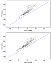Fig. A.1. Comparison of the FUV and NUV measurements from Bellstedt et al. (2020) for GAMA and Bianchi et al. (2011) for SDSS of galaxies appearing in both SDSS and GAMA. The blue line shows the one-to-one relation for the different bands. The figure shows that the measurements do not align, meaning we need to decide which photometry we trust the most for our calibrations.

The comparison shows that the FUV and NUV have a constant offset in magnitudes of ∼1.2 ± 0.8 and ∼1.0 ± 0.6 respectively, whereas the optical and NIR magnitudes (not shown) are in agreement with each other. The UV offset is independent of galaxy inclination (Fig. A.2) and g-band half-light radius (Fig. A.3), meaning it is likely independent of the size and shape of the aperture used in the Bellstedt et al. (2020) derivations. Due to the updated method used in the new GAMA photometry, we have decided to correct the SDSS GALEX UV MIS magnitudes by subtracting the offset.

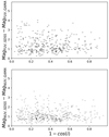Fig. A.2. FUV (top) and NUV (bottom) measurement comparison of Bellstedt et al. (2020, GAMA) and Bianchi et al. (2011, SDSS) photometry for galaxies appearing in both surveys as a function of inclination 1 − cos(i). The figure shows that the difference in photometry is independent of inclination.

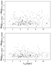Fig. A.3. FUV and NUV measurement comparison from Bellstedt et al. (2020) for GAMA and Bianchi et al. (2011) for SDSS of galaxies appearing in both SDSS and GAMA as a function of half-light radius r1/2. The figure shows that the difference in photometry is independent of r1/2.

Appendix B: Fitting bulge-to-total ratio

One of the model parameters from the T04 model is the bulge-to-total ratio r_bulge, which tells us about how the radiation is divided between the bulge and the disks. The impact of the parameter on Δm is dependent on inclination, which could influence the accuracy of our results as such effects can also be caused by the ${\tau }_B^f$. Studies such as Häußler et al. (2013) and Simard et al. (2002) used different methods to constrain the ratio. As mentioned in Sect. 3, we derive the distribution of the bulge-to-total ratio derived for our selected star-forming galaxies in GAMA and COSMOS to act as the prior for the T04 model fitting.

We first select star-forming galaxies from the GAMA sample following Sect. 2.4.1 and only use the galaxies which can be found in SDSS to use the derived bulge-to-total ratios from Simard et al. (2011). For COSMOS, we select star-forming galaxies following Sect. 2.4.1 and use the bulge-to-total ratios from the CANDELS data set (Häußler et al. 2013). We use scikit.learn to fit r_bulge as a function of M_*, r_1/2, and g − r color. We assume that the ratio follows a power law in both parameters and apply the linear regression module to derive the relations. In Figs. B.1 and B.2, we show the fitting results and show that, together, these three variables give good results in predicting the r_bulge.

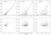Fig. B.1. Bulge-to-total ratio B/T of galaxies appearing in both SDSS and GAMA against the Sérsic index n, M* and g − r color. The blue line shows the best-fit model where we change the variable per plot: top-left is for varying n, top-middle is for varying M* and top right is for varying g − r. The bottom plots illustrate the residuals of the data – model for each data point.

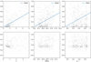Fig. B.2. Bulge-to-total ratio B/T of galaxies appearing in COSMOS and CANDELS against the Sérsic index n, M* and B − V color. The blue line shows the best-fit model where we change the variable per panel: top-left is for varying n, top-middle is for varying M* and top right is for varying B − V. The bottom panels illustrate the residuals of the data – model for each galaxy. The model seems to mostly agree but tends to underestimate B/T for higher values of the galaxy properties.

Appendix C: Importance sampling

Our analysis relies on unbiased photometry and galaxies with similar properties that do not vary in inclination. We have found in Sect. 2.4.2 that the physical properties derived from photometry have an implicit relation with inclination. The inclination dependence hints at an inclination bias in our photometry that might come from detection bias and could interfere with the attenuation-inclination trends we want to analyze. The inclination bias of the physical properties gives us insight into how the inclination biases our photometry and, therefore, the selected galaxy distribution. Importance sampling uses this information to correct the biases. We refer readers to Chevallard et al. (2013) for an overview. In this section, we describe the basic principles needed to understand the implementation of the technique in our analyses.

Importance sampling is a statistical technique that corrects for implicit biases in datasets. This technique comes from the mathematical description of finding expected values with a distribution of observable x:

$$\begin{array}{c}\hfill \overline{x}={\displaystyle \int }xf(x)\mathrm{d}x,\end{array}$$(C.1)

where f(x) is the probability function of observable x and $\overline{x}$ the average value of the observable. Importance sampling is a result of rewriting Eq. (C.1) as:

$$\begin{array}{c}\hfill \overline{x}={\displaystyle \int }x\frac{f(x)}{g(x)}g(x)\mathrm{d}x,\end{array}$$(C.2)

with f(x) and g(x) both being different probability distributions, allowing us to transform between distributions of parameters. The transformation for our case is between the observed distribution, represented by g(x) and the inclination unbiased distribution f(x). Since we are dealing with discrete measurements, we rewrite Eq. (C.2) as a sum instead of an integral:

$$\begin{array}{c}\hfill \overline{x}=\frac{{\mathrm{\Sigma }}_{i}x\frac{f(x)}{g(x|y_i)}}{\mathrm{\Sigma }\frac{f(x)}{g(x|y_i)}},\end{array}$$(C.3)

with x being the observed physical property and g(x|y_i) being the probability function for x, given a known y, in our case, the inclination. The ratio $\frac{f(x)}{g(x|y_i)}$ represent weights that describes how much the measurement of distribution f(x) would contribute to the mean if the data would be drawn from a different distribution g(x). We need to calculate the weights to ensure that the averages we calculate in photometry are unbiased by the inclination before deriving the inclination dependent model parameters.

The physical properties that show inclination bias are log(M_*), r_1/2, and n. We add redshift z to the list to take into account possible cosmological volume corrections to create one weight per galaxy. For each property, we derive the distribution per inclination bin by separating the galaxies into ten bins of inclination angle. In each bin, we assume a Gaussian distribution for the physical properties and determine distributions using the Gaussian kernel density estimator provided in the scipy package. We refer to the distributions of single physical property as h(x|y). The global probability distribution g(x|y) is found by multiplying the single probability distribution with each other:

$$\begin{array}{c}\hfill g(x|y)={\displaystyle \prod _j^n{h}_j(x_j|\mathrm{y}),}\end{array}$$(C.4)

with h_j(x_j|y) being the probability function of the physical properties, assuming the properties are independent.

We cannot define an inclination unbiased distribution f(x) because each bin could be inclination biased. Therefore, we follow Chevallard et al. (2013) for calculating the inclination unbiased distribution:

$$\begin{array}{c}\hfill f(x)={\displaystyle \prod _i{g}_i{(x|y_i)}^{0.1}.}\end{array}$$(C.5)

With this relation, we use both f(x) and g(x|y) to calculate the weights $\frac{f(x)}{g(x|y_i)}$ that we apply to the photometry to calculate unbiased mean values.

Appendix D: Testing model fidelity

The decisions made in Sect. 3, such as the face-on normalization of optical emission, could influence the accuracy of our fitting results, causing small offsets in fitting for the best-fit parameters. In this section, we investigate how any offset influences our results. The analysis was done using simulated attenuation-inclination curves from the T04 model in the GALEX FUV & NUV bands, B, V, and I bands, and 2MASS J and K bands without adding any uncertainty. We simulate attenuation-inclination for different values of ${\tau }_B^f$, F and r_bulge and apply our fitting regime on the models. When varying the one of the parameters, we fix the other two to default values of ${\tau }_B^f=4.0$, F = 0.3, and r_bulge = 0.5.

D.1. Face-on normalization

First, we show the impact of the normalization in the optical bands on our results. Since we cannot estimate the intrinsic emission in optical and NIR bands, we normalize these bands by the average value of galaxies with inclination 0.1 < 1 − cos(i) < 0.2. The results of the model fitting compared to our input are given in Fig. D.1. For each panel, we only vary one of the three parameters. The two parameters we leave as constant are set on the values given in Sect. D.

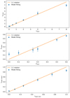Fig. D.1. Comparison between the input parameters used to create the T04 model from which simulated NIR to UV attenuation-inclination relations were drawn, and the resulting best-fit parameter. The blue points show the results of the fitting using different values of ${\tau }_B^f$, F and rbulge, the orange line is the one−to−one relation. We see that the offset increases the closer the parameters. For each panel, we only vary one of the three parameters. The other two parameters are set to the values given in Sect. D. The figure shows that the fitting result will differ based on how close the model is to the boundaries defined by the prior.

In Fig. D.1 we see that there is an offset for the model fitted parameters at different input for ${\tau }_B^f$, F and r_bulge. This offset is mostly driven by the priors and the distribution of samplers. The distribution of parameters has a Poisson distribution. The median value of the distribution is dependent on the boundaries, as the distribution becomes skewed at the boundaries, meaning the median value has a slight offset. For F, we also have the influence of ${\tau }_B^f$. The vertical offset in the attenuation-inclination relation in UV is dependent on F and ${\tau }_B^f$. Low values of F mean that the offset is very small. This causes the fitting for low values of F to be very uncertain and is often paired with increased uncertainty in ${\tau }_B^f$ because the small vertical offset could also be explained by a change in ${\tau }_B^f$.

D.2. Sensitivity of the bands

Next, we cover the number of photometric bands used, as this is a key difference between our work and Leslie et al. (2018a). Leslie et al. (2018a) used only the GALEX FUV bands to find the best-fit value for ${\tau }_B^f$ and F, whereas we use GALEX FUV and NUV together with BVIJK for COSMOS and SDSS griJK for SDSS and GAMA. We model attenuation-inclination relations using the T04 model for several combinations of ${\tau }_B^f$, F and r_bulge. We apply the model fitting using separate bands and compare this best-fit parameter from each band with the best-fit parameter using all the bands. The results are given in Fig. D.2, where we only vary one of the three parameters for each panel.

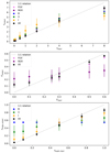Fig. D.2. Comparison between the input parameters used to create the T04 model and the resulting best-fit parameter using the T04 model in different bands. The accuracy of the fitting is dependent on how much the band is affected by attenuation. Using all the bands gives the best results.

In Fig. D.2 we see the fitting results for different values of ${\tau }_B^f$, F and r_bulge using different bands. We know that the UV bands are more affected by attenuation than the optical bands are. This difference in sensitivity means that the ${\tau }_B^f$ found from UV bands should be more accurate than the optical bands, which we see in the top panel. In the middle panel, we see the FUV results obtaining the F very well, whereas the NUV results show a larger offset closer to the priors. This difference is due to the FUV being more sensitive to F compared to NUV. In the bottom panel, we see that the I-band has the closest best-fit results to the input values of r_bulge. The I-band magnitude is not very affected by the inclination effects of the diffuse dust from the disks, making the inclination dependence primarily driven by r_bulge. This dependence should, in turn, mean that bands that are more affected by the diffuse dust will find less accurate results for the fitted r_bulge, which is also what we see. For both ${\tau }_B^f$, F and r_bulge we see that using all bands gives the best fit, as this takes all the previously mentioned effects into account, similar to what we found when comparing our results with Leslie et al. (2018a).

Appendix E: Estimating intrinsic UV emission

In this study, we derived intrinsic emission by correcting the GALEX FUV and NUV bands using MIR emission following Hao et al. (2011). In Leslie et al. (2018a), they used different methods of deriving the intrinsic FUV emission based on the star-formation main-sequence. The star-formation main-sequence is highly dependent on sample selection, resulting in multiple papers with different SFR − M_* relations. Here, we discuss the three different star-formation main-sequences used to derive intrinsic UV emission in Leslie et al. (2018a) and how they impact the model fitting results.

E.1. Star-formation main-sequence

The main star-formation main-sequence (SF MS) used in Leslie et al. (2018a), is derived from an updated sample presented in Sargent et al. (2014):

$$\begin{array}{c}\hfill log\left(\frac{{\mathrm{SFR}}_{\mathrm{MS}}}{M_{\odot {\mathrm{yr}}^{-1}}}\right)=0.816log\left(\frac{M_{\ast }}{M_{\odot }}\right)-8.248+3log(1+z),\end{array}$$(E.1)

with SFR_MS the star-formation rate of a main-sequence galaxy, and z the corresponding redshift. Appendix A of Leslie et al. (2018a) also shows results using two additional main-sequences: the Speagle et al. (2014) best-fit main-sequence derived by compiling 25 different literary works, and the Schreiber et al. (2015) main-sequence, derived using a stacking analysis of star-forming galaxies, combining UV and FIR data. The Speagle et al. (2014) is given as:

$$\begin{array}{c}\hfill log\left(\frac{{\mathrm{SFR}}_{\mathrm{MS}}}{M_{\odot {\mathrm{yr}}^{-1}}}\right)=(0.84-0.026t)log\left(\frac{M_{\ast }}{M_{\odot }}\right)-(6.51-0.11t),\end{array}$$(E.2)

with t the age of the Universe in Gyr and assuming a Kroupa IMF. The Schreiber et al. (2015) MS is given as:

$$\begin{array}{c}\hfill \begin{array}{cc}\hfill log\left(\frac{{\mathrm{SFR}}_{\mathrm{MS}}}{M_{\odot {\mathrm{yr}}^{-1}}}\right)& =m-0.5+1.5log(1+z)\hfill \\ \hfill & -0.3{[max(0,m-0.36-2.5log(1+z))]}^2,\hfill \end{array}\end{array}$$(E.3)

where $m=\frac{M_{\ast }}{{10}^9{M}_{\odot }}$.

E.2. From SFR to UV

We use the Kennicutt & Evans (2012) conversions to derive the expected intrinsic emission:

$$\begin{array}{c}\hfill {\mathrm{SFR}}_{\mathrm{MS}}=C_{\nu }\nu L_{\nu }.\end{array}$$(E.4)

The assumption needed to use the conversion in our analysis is that all galaxies in our sample are main-sequence galaxies. We derive the SFR from the different star-formation main-sequences and convert the SFRs to FUV and NUV luminosities. Since the T04 models normalize by the intrinsic magnitudes rather than the intrinsic luminosities, we apply the conversion to magnitudes and follow the same procedure as Sect. 3.

E.3. Fitting comparison

We use the same fitting regime as in the main analysis to obtain the best-fit parameters for the τ_B, F, and bulge fraction. We show the best-fit values from the magnitude-inclination relation of all galaxies in Fig. E.1 and for galaxies binned by SFR in Fig. E.2.

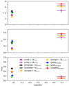Fig. E.1. Results of fitting the T04 model for galaxies in the GAMA, SDSS and COSMOS datasets using different assumptions for the intrinsic UV emission. The fitted parameters are the ${\tau }_B^f$ (top), F (middle), and rbulge (bottom). The assumptions for intrinsic emission are made using different star-formation main-sequences: Leslie et al. (2018a) (purple), Schreiber et al. (2015) (green), and Speagle et al. (2014) (orange), where square markers indicate the sample around z ≈ 0.0 and the crosses for the sample around z ≈ 0.7. We see that in all cases ${\tau }_B^f$ and F increase with redshift, with the different assumptions only shifting the value.

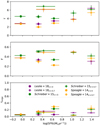Fig. E.2. Results of fitting the T04 model for galaxies in the GAMA, SDSS and COSMOS datasets using different assumptions for the intrinsic emission separated in bins of SFR. The fitted parameters are the ${\tau }_B^f$ (top), F (middle), and rbulge (bottom). The assumptions for intrinsic emission are made using different star-formation main-sequences: Leslie et al. (2018a) (purple), Schreiber et al. (2015) (green), and Speagle et al. (2014) (orange), where square markers indicate the sample around z ≈ 0.0 and the crosses for the sample around z ≈ 0.7. We see that none of the normalizations result in a consistent trend between SFR and any of the fitted parameters.

Figure E.1 shows that the results for the low-z galaxies are consistent across the different intrinsic corrections, whereas the fitting for the z ∼ 0.7 galaxies has different fitted values. Figure E.1, for instance, shows that Leslie et al. (2018a) obtains lower ${\tau }_B^f$ for z ≈ 0.7 galaxies, where our results in Fig. 4 are in line with the higher ${\tau }_B^f.$ The trends over redshift remain qualitatively the same, meaning that the star-formation main-sequence has a negligible impact on the redshift evolution. The main-sequence starts to have more influence on the results when we study the dependence on SFR. The trends remain inconsistent, which could mean that either the uncertainty in SFR causes the inconsistency or that the SFR and dust parameters are independent. The inconsistent trends in these results may be an indirect result of us assuming intrinsic emission based on the SFR following Kennicutt & Evans (2012). The relation between intrinsic UV emission and SFR have all been estimated using the Starburst99 stellar evolution models (Leitherer et al. 1999) assuming a Chabrier IMF, solar abundances, and constant star-formation on 100 Myr timescales. When we bin our galaxies based on a property, we confirm that the remaining properties investigated remain constant between the bins. However, we cannot check how the metallicity or star-formation histories vary between our sample bins. Therefore, we cannot confirm whether the assumptions made for the Kennicutt & Evans (2012) calibration are valid, and this may add systematic uncertainties to our findings. The inconsistent results when applying different main-sequence relations could also hint at the variation in the star-forming galaxy selection used to derive the different main-sequence relations. Thus, we can not confirm that the main-sequence combined with the Kennicutt & Evans (2012) SFR calibration is an appropriate method for deriving the intrinsic UV emission of main-sequence galaxies and adopt the MIR correction for our main analyses.

All Tables

All Figures

Fig. 1. Distributions of the inclination corrected properties of star-forming galaxies in the three galaxy datasets SDSS, GAMA, and COSMOS, based on the different rest-frame detection criteria. The criteria are: (1) the galaxy is detected in at least one band (black), (2) the galaxy is detected in at least one UV band, one optical, one NIR, and one MIR band with S/N > 3 (blue), (3) the galaxy is detected in at least one UV band with S/N > 3 (red), (4) the galaxy is detected in at least one optical band with S/N > 3 (yellow), (5) the galaxy is detected in at least one NIR band with S/N > 3 (green), (6) the galaxy is detected in at least one MIR band with S/N > 3 (purple). The properties are, from top to bottom, inclination 1 − cos(i), redshift z, stellar mass log(M*), half-light radius r1/2, Sérsic index n and stellar mass surface density μ*. In general, the UV selection affects the number of galaxies detected in all samples. Most of the differences in selections are not visible, as the distributions overlap with each other. There is a bias toward more massive galaxies when requiring a MIR-detection in COSMOS.

In the text

	Fig. 2. Rest-frame NUV − r and r − J color diagram of galaxies used before (gray) and after (colored) applying the selection in star-formation classification and physical properties log(M*) and n, including AGN removal. We select star-forming galaxies to lie below the black line.
In the text

Fig. 3. Magnitude-inclination relations. Top row: inclination distribution of all selected star-forming galaxies in the three samples. The other panels show the magnitude-inclination relation for SDSS, GAMA, and COSMOS in rest-frame UV, optical, and NIR bands. The grayscale is a 2D histogram of all the galaxies with a signal-to-noise ratio > 3 in the respective band and the blue points show the mean values with the 32–68th percentile as errors in 10 bins of inclination using the importance sampling weights. We note that our sample selection does not require a galaxy to be detected in all photometric bands.

In the text

Fig. 4. Results of fitting the T04 model for galaxies in the GAMA, SDSS, and COSMOS datasets. The fitted parameters are the ${\tau }_B^f$ (top), F (middle), and rbulge (bottom). We compare the fitted values of ${\tau }_B^f$ and F to the ones found in Leslie et al. (2018a), Driver et al. (2007), and Andrae et al. (2012), and the fitted values for rbulge to the average and 32–68th percentile of the bulge-to-total distribution of the selected samples, labeled with the subscript “data”. Our best-fit values are in line with the literature values. We see that ${\tau }_B^f$ and F increase with redshift.

In the text

	Fig. 5. Results of the MCMC sampling and the best-fit parameter distributions using the T04 attenuation-inclination model. We show the fitting results for galaxies in SDSS (green), GAMA (blue), and COSMOS (red) datasets. We compare the fitted values for rbulge to the average and 32–68th percentile of the bulge-to-total distribution of the selected samples, labeled as data.
In the text

	Fig. 6. Distributions of our selected star-forming galaxy samples in SDSS, GAMA, and COSMOS. The figure shows the distribution in μ* (left panel), and SFR (right panel). As the COSMOS sample is selected at higher redshift, we convert the SFR to redshift z = 0 assuming that SFR ≈ (1 + z)3. Black lines show the boundaries of the bins used in our analyses.
In the text

	Fig. 7. Best-fit values for ${\tau }_B^f$, F and rbulge for galaxies in our datasets, divided in bins of log(M*[M⊙]). We compare the fitted values for rbulge to the average and 32–68th percentile of the bulge-to-total distribution of the selected samples, labeled with the subscript “data”.
In the text

Fig. 8. Best-fit values for ${\tau }_B^f$, F and rbulge for galaxies in our datasets, divided in bins of μ*. We compare the fitted values for rbulge to the average and 32–68th percentile of the bulge-to-total distribution of the selected samples, labeled with the subscript “data”. The results show an increase ${\tau }_B^f$ for an increase in μ*, similar to Grootes et al. (2013), given by the black dashed line and gray. The GAMA and COSMOS surveys do not contain enough high surface density galaxies to describe a clear magnitude-inclination relation, resulting in the model not obtaining fitting results at log(μ∗) ∼ 8.7 M⊙ kpc−2.

In the text

	Fig. 9. Best-fit values for ${\tau }_B^f$, F and rbulge for galaxies in our datasets, divided in bins of SFR. We compare the fitted values for rbulge to the average and 32–68th percentile of the bulge-to-total distribution of the selected samples, labeled with the subscript “data”. The best-fit parameters do not show a consistent correlation overall.
In the text

	Fig. 10. Best-fit values for ${\tau }_B^f$, F and rbulge for galaxies in our datasets, divided in bins of sSFR. We compare the fitted values for rbulge to the average and 32–68th percentile of the bulge-to-total distribution of the selected samples, labeled as data.
In the text

	Fig. 11. Best-fit values for ${\tau }_B^f$, F and rbulge for galaxies in our datasets, divided in bins of dMS. We compare the fitted values for rbulge to the average and 32–68th percentile of the bulge-to-total distribution of the selected samples, labeled as data.
In the text

	Fig. 12. Best-fit values for ${\tau }_B^f$, F and rbulge for galaxies in our datasets, divided in bins of ΣSFR. We compare the fitted values for rbulge to the average and 32–68th percentile of the bulge-to-total distribution of the selected samples, labeled as data.
In the text

	Fig. 13. Hα/Hβ ratio for the SDSS and GAMA sample for galaxies with varying inclination. Top two panels: inclination distribution, and the bottom two panels show the Hα/Hβ – inclination relation for the selected star-forming sample and the Hα/Hβ ratio – inclination relation from the T04 model with varying ${\tau }_B^f$. We can see that none of the T04 models can describe the observed trend.
In the text

	Fig. 14. Best-fit values for ${\tau }_B^f$, F, rbulge, and C for galaxies in our datasets, divided in bins of mass log(M*[M⊙]).
In the text

Fig. 15. Evolution of massive galaxy properties from their low-z values out to z ∼ 1. Relationships for molecular gas to stellar mass ratio (MH2/M*), specific SFR, SFR efficiency (SFR/MH2), and metallicity (log(O/H)+12) are from the A3COSMOS scaling relations for main-sequence galaxies derived by Liu et al. (2019), adopting the Schreiber et al. (2015) main-sequence. Solid lines show the relations at log(M*/M⊙) = 10.2 and dotted lines show the relations for galaxies with log(M*/M⊙) = 11.5. Unlike (Leslie et al. 2018a, L18), who found that F increases with redshift and the τB ${\tau }_B^f$ remains constant to z ∼ 0.7, we find that both these dust parameters evolve together increasing by a factor of ∼1.7 (${\tau }_B^f$) and ∼1.8 (F) from low-z galaxies in GAMA and SDSS to intermediate-redshift galaxies in COSMOS.

In the text

	Fig. A.1. Comparison of the FUV and NUV measurements from Bellstedt et al. (2020) for GAMA and Bianchi et al. (2011) for SDSS of galaxies appearing in both SDSS and GAMA. The blue line shows the one-to-one relation for the different bands. The figure shows that the measurements do not align, meaning we need to decide which photometry we trust the most for our calibrations.
In the text

	Fig. A.2. FUV (top) and NUV (bottom) measurement comparison of Bellstedt et al. (2020, GAMA) and Bianchi et al. (2011, SDSS) photometry for galaxies appearing in both surveys as a function of inclination 1 − cos(i). The figure shows that the difference in photometry is independent of inclination.
In the text

	Fig. A.3. FUV and NUV measurement comparison from Bellstedt et al. (2020) for GAMA and Bianchi et al. (2011) for SDSS of galaxies appearing in both SDSS and GAMA as a function of half-light radius r1/2. The figure shows that the difference in photometry is independent of r1/2.
In the text

	Fig. B.1. Bulge-to-total ratio B/T of galaxies appearing in both SDSS and GAMA against the Sérsic index n, M* and g − r color. The blue line shows the best-fit model where we change the variable per plot: top-left is for varying n, top-middle is for varying M* and top right is for varying g − r. The bottom plots illustrate the residuals of the data – model for each data point.
In the text

Fig. B.2. Bulge-to-total ratio B/T of galaxies appearing in COSMOS and CANDELS against the Sérsic index n, M* and B − V color. The blue line shows the best-fit model where we change the variable per panel: top-left is for varying n, top-middle is for varying M* and top right is for varying B − V. The bottom panels illustrate the residuals of the data – model for each galaxy. The model seems to mostly agree but tends to underestimate B/T for higher values of the galaxy properties.

In the text

Fig. D.1. Comparison between the input parameters used to create the T04 model from which simulated NIR to UV attenuation-inclination relations were drawn, and the resulting best-fit parameter. The blue points show the results of the fitting using different values of ${\tau }_B^f$, F and rbulge, the orange line is the one−to−one relation. We see that the offset increases the closer the parameters. For each panel, we only vary one of the three parameters. The other two parameters are set to the values given in Sect. D. The figure shows that the fitting result will differ based on how close the model is to the boundaries defined by the prior.

In the text

	Fig. D.2. Comparison between the input parameters used to create the T04 model and the resulting best-fit parameter using the T04 model in different bands. The accuracy of the fitting is dependent on how much the band is affected by attenuation. Using all the bands gives the best results.
In the text

Fig. E.1. Results of fitting the T04 model for galaxies in the GAMA, SDSS and COSMOS datasets using different assumptions for the intrinsic UV emission. The fitted parameters are the ${\tau }_B^f$ (top), F (middle), and rbulge (bottom). The assumptions for intrinsic emission are made using different star-formation main-sequences: Leslie et al. (2018a) (purple), Schreiber et al. (2015) (green), and Speagle et al. (2014) (orange), where square markers indicate the sample around z ≈ 0.0 and the crosses for the sample around z ≈ 0.7. We see that in all cases ${\tau }_B^f$ and F increase with redshift, with the different assumptions only shifting the value.

In the text

Fig. E.2. Results of fitting the T04 model for galaxies in the GAMA, SDSS and COSMOS datasets using different assumptions for the intrinsic emission separated in bins of SFR. The fitted parameters are the ${\tau }_B^f$ (top), F (middle), and rbulge (bottom). The assumptions for intrinsic emission are made using different star-formation main-sequences: Leslie et al. (2018a) (purple), Schreiber et al. (2015) (green), and Speagle et al. (2014) (orange), where square markers indicate the sample around z ≈ 0.0 and the crosses for the sample around z ≈ 0.7. We see that none of the normalizations result in a consistent trend between SFR and any of the fitted parameters.

In the text

References

- Abazajian, K. N., Adelman-McCarthy, J. K., Agüeros, M. A., et al. 2009, ApJS, 182, 543 [Google Scholar]
- Alton, P. B., Trewhella, M., Davies, J. I., et al. 1998, A&A, 335, 807 [NASA ADS] [Google Scholar]
- Andrae, E., Tuffs, R. J., Popescu, C. C., & Seibert, M. 2012, in The Spectral Energy Distribution of Galaxies – SED 2011, ed. R. J. Tuffs, IAU Symp., 284, 312 [Google Scholar]
- Arnouts, S., Moscardini, L., Vanzella, E., et al. 2002, MNRAS, 329, 355 [Google Scholar]
- Assef, R. J., Prieto, J. L., Stern, D., et al. 2018, ApJ, 866, 26 [NASA ADS] [CrossRef] [Google Scholar]
- Baldry, I. K., Liske, J., Brown, M. J. I., et al. 2018, MNRAS, 474, 3875 [Google Scholar]
- Battisti, A. J., Calzetti, D., & Chary, R. R. 2016, ApJ, 818, 13 [NASA ADS] [CrossRef] [Google Scholar]
- Battisti, A. J., Calzetti, D., & Chary, R. R. 2017, ApJ, 851, 90 [NASA ADS] [CrossRef] [Google Scholar]
- Bellstedt, S., Driver, S. P., Robotham, A. S. G., et al. 2020, MNRAS, 496, 3235 [NASA ADS] [CrossRef] [Google Scholar]
- Béthermin, M., Daddi, E., Magdis, G., et al. 2015, A&A, 573, A113 [Google Scholar]
- Bianchi, S. 2007, A&A, 471, 765 [NASA ADS] [CrossRef] [EDP Sciences] [Google Scholar]
- Bianchi, L., Herald, J., Efremova, B., et al. 2011, Ap&SS, 335, 161 [Google Scholar]
- Bigiel, F., Leroy, A., Walter, F., et al. 2008, AJ, 136, 2846 [NASA ADS] [CrossRef] [Google Scholar]
- Blanton, M. R., & Roweis, S. 2007, AJ, 133, 734 [NASA ADS] [CrossRef] [Google Scholar]
- Blanton, M. R., Schlegel, D. J., Strauss, M. A., et al. 2005, AJ, 129, 2562 [NASA ADS] [CrossRef] [Google Scholar]
- Boquien, M., Buat, V., Boselli, A., et al. 2012, A&A, 539, A145 [NASA ADS] [CrossRef] [EDP Sciences] [Google Scholar]
- Boquien, M., Burgarella, D., Roehlly, Y., et al. 2019, A&A, 622, A103 [NASA ADS] [CrossRef] [EDP Sciences] [Google Scholar]
- Brinchmann, J., Charlot, S., White, S. D. M., et al. 2004, MNRAS, 351, 1151 [Google Scholar]
- Bruzual, G., & Charlot, S. 2003, MNRAS, 344, 1000 [NASA ADS] [CrossRef] [Google Scholar]
- Burkert, A., Förster Schreiber, N. M., Genzel, R., et al. 2016, ApJ, 826, 214 [Google Scholar]
- Calura, F., Pozzi, F., Cresci, G., et al. 2017, MNRAS, 465, 54 [Google Scholar]
- Calzetti, D. 1996, in New Extragalactic Perspectives in the New South Africa, eds. D. L. Block, & J. M. Greenberg, Astrophys. Space Sci. Lib., 209, 271 [NASA ADS] [CrossRef] [Google Scholar]
- Calzetti, D. 1997, AJ, 113, 162 [NASA ADS] [CrossRef] [Google Scholar]
- Calzetti, D. 2001, PASP, 113, 1449 [Google Scholar]
- Casasola, V., Hunt, L., Combes, F., & García-Burillo, S. 2015, A&A, 577, A135 [NASA ADS] [CrossRef] [EDP Sciences] [Google Scholar]
- Casasola, V., Cassarà, L. P., Bianchi, S., et al. 2017, A&A, 605, A18 [NASA ADS] [CrossRef] [EDP Sciences] [Google Scholar]
- Casasola, V., Bianchi, S., De Vis, P., et al. 2020, A&A, 633, A100 [NASA ADS] [CrossRef] [EDP Sciences] [Google Scholar]
- Catalán-Torrecilla, C., Gil de Paz, A., Castillo-Morales, A., et al. 2015, A&A, 584, A87 [NASA ADS] [CrossRef] [EDP Sciences] [Google Scholar]
- Chabrier, G. 2003, PASP, 115, 763 [Google Scholar]
- Chang, Y.-Y., van der Wel, A., da Cunha, E., & Rix, H.-W. 2015, ApJS, 219, 8 [Google Scholar]
- Charlot, S., & Fall, S. M. 2000, ApJ, 539, 718 [Google Scholar]
- Chevallard, J., Charlot, S., Wandelt, B., & Wild, V. 2013, MNRAS, 432, 2061 [CrossRef] [Google Scholar]
- Civano, F., Marchesi, S., Comastri, A., et al. 2016, ApJ, 819, 62 [Google Scholar]
- Clemens, M. S., Negrello, M., De Zotti, G., et al. 2013, MNRAS, 433, 695 [NASA ADS] [CrossRef] [Google Scholar]
- Cluver, M. E., Jarrett, T. H., Hopkins, A. M., et al. 2014, ApJ, 782, 90 [Google Scholar]
- Cluver, M. E., Jarrett, T. H., Dale, D. A., et al. 2017, ApJ, 850, 68 [Google Scholar]
- Conroy, C. 2010, MNRAS, 404, 247 [Google Scholar]
- Corbelli, E., Bianchi, S., Cortese, L., et al. 2012, A&A, 542, A32 [NASA ADS] [CrossRef] [EDP Sciences] [Google Scholar]
- Cortese, L., Ciesla, L., Boselli, A., et al. 2012, A&A, 540, A52 [NASA ADS] [CrossRef] [EDP Sciences] [Google Scholar]
- da Cunha, E., Charlot, S., & Elbaz, D. 2008, MNRAS, 388, 1595 [Google Scholar]
- da Cunha, E., Eminian, C., Charlot, S., & Blaizot, J. 2010, MNRAS, 403, 1894 [Google Scholar]
- Davies, R. I., Hicks, E. K. S., Erwin, P., et al. 2017, MNRAS, 466, 4917 [Google Scholar]
- de Jong, J. T. A., Verdoes Kleijn, G. A., Kuijken, K. H., & Valentijn, E. A. 2013, Exp. Astron., 35, 25 [Google Scholar]
- De Vis, P., Dunne, L., Maddox, S., et al. 2017, MNRAS, 464, 4680 [NASA ADS] [CrossRef] [Google Scholar]
- Donley, J. L., Koekemoer, A. M., Brusa, M., et al. 2012, ApJ, 748, 142 [Google Scholar]
- Draine, B. T., & Li, A. 2007, ApJ, 657, 810 [CrossRef] [Google Scholar]
- Draine, B. T., Dale, D. A., Bendo, G., et al. 2007, ApJ, 663, 866 [NASA ADS] [CrossRef] [Google Scholar]
- Driver, S. P. 2015, ArXiv e-prints [arXiv:1507.00665] [Google Scholar]
- Driver, S. P., Popescu, C. C., Tuffs, R. J., et al. 2007, MNRAS, 379, 1022 [NASA ADS] [CrossRef] [Google Scholar]
- Driver, S. P., Norberg, P., Baldry, I. K., et al. 2009, Astron. Geophys., 50, 5 [Google Scholar]
- Edge, A., Sutherland, W., Kuijken, K., et al. 2013, The Messenger, 154, 32 [NASA ADS] [Google Scholar]
- Ellison, S. L., Thorp, M. D., Lin, L., et al. 2020, MNRAS, 493, L39 [CrossRef] [Google Scholar]
- Foreman-Mackey, D., Conley, A., Meierjurgen Farr, W., et al. 2013, PASP, 125, 306 [NASA ADS] [CrossRef] [Google Scholar]
- Galliano, F., Dwek, E., & Chanial, P. 2008, ApJ, 672, 214 [NASA ADS] [CrossRef] [Google Scholar]
- Gordon, K. D., Misselt, K. A., Witt, A. N., & Clayton, G. C. 2001, ApJ, 551, 269 [NASA ADS] [CrossRef] [Google Scholar]
- Gordon, Y. A., Owers, M. S., Pimbblet, K. A., et al. 2017, MNRAS, 465, 2671 [NASA ADS] [CrossRef] [Google Scholar]
- Grootes, M. W., Tuffs, R. J., Popescu, C. C., et al. 2013, ApJ, 766, 59 [NASA ADS] [CrossRef] [Google Scholar]
- Groves, B. A., Schinnerer, E., Leroy, A., et al. 2015, ApJ, 799, 96 [Google Scholar]
- Hao, C.-N., Kennicutt, R. C., Johnson, B. D., et al. 2011, ApJ, 741, 124 [Google Scholar]
- Häußler, B., Bamford, S. P., Vika, M., et al. 2013, MNRAS, 430, 330 [Google Scholar]
- Hill, D. T., Kelvin, L. S., Driver, S. P., et al. 2011, MNRAS, 412, 765 [NASA ADS] [Google Scholar]
- Hodge, J. A., Smail, I., Walter, F., et al. 2019, ApJ, 876, 130 [Google Scholar]
- Holmberg, E. 1958, Meddelanden fran Lunds Astronomiska Observatorium Serie II, 136, 1 [Google Scholar]
- Hunt, L. K., Draine, B. T., Bianchi, S., et al. 2015, A&A, 576, A33 [NASA ADS] [CrossRef] [EDP Sciences] [Google Scholar]
- Ilbert, O., Arnouts, S., McCracken, H. J., et al. 2006, A&A, 457, 841 [NASA ADS] [CrossRef] [EDP Sciences] [Google Scholar]
- Ilbert, O., McCracken, H. J., Le Fèvre, O., et al. 2013, A&A, 556, A55 [NASA ADS] [CrossRef] [EDP Sciences] [Google Scholar]
- Ilbert, O., Arnouts, S., Le Floc’h, E., et al. 2015, A&A, 579, A2 [NASA ADS] [CrossRef] [EDP Sciences] [Google Scholar]
- Inoue, S., & Yoshida, N. 2019, MNRAS, 488, 4400 [NASA ADS] [CrossRef] [Google Scholar]
- Jonsson, P. 2006, MNRAS, 372, 2 [NASA ADS] [CrossRef] [Google Scholar]
- Jonsson, P., Groves, B. A., & Cox, T. J. 2010, MNRAS, 403, 17 [NASA ADS] [CrossRef] [Google Scholar]
- Kampczyk, P., Lilly, S. J., Carollo, C. M., et al. 2007, ApJS, 172, 329 [NASA ADS] [CrossRef] [Google Scholar]
- Kauffmann, G., Heckman, T. M., White, S. D. M., et al. 2003, MNRAS, 341, 33 [Google Scholar]
- Kelvin, L. S., Driver, S. P., Robotham, A. S. G., et al. 2012, MNRAS, 421, 1007 [Google Scholar]
- Kennicutt, R. C., Jr 1998, ApJ, 498, 541 [Google Scholar]
- Kennicutt, R. C., Jr, & De Los Reyes, M. A. C. 2021, ApJ, 908, 61 [NASA ADS] [CrossRef] [Google Scholar]
- Kennicutt, R. C., Jr, & Evans, N. J. 2012, ARA&A, 50, 531 [NASA ADS] [CrossRef] [Google Scholar]
- Kennicutt, R. C., Jr, Hao, C.-N., Calzetti, D., et al. 2009, ApJ, 703, 1672 [NASA ADS] [CrossRef] [Google Scholar]
- Kewley, L. J., Groves, B., Kauffmann, G., & Heckman, T. 2006, MNRAS, 372, 961 [Google Scholar]
- Koekemoer, A. M., Aussel, H., Calzetti, D., et al. 2007, ApJS, 172, 196 [Google Scholar]
- Kokorev, V., Magdis, G., Davidzon, I., et al. 2021, ApJ, 921, 40 [NASA ADS] [CrossRef] [Google Scholar]
- Kroupa, P. 2001, MNRAS, 322, 231 [NASA ADS] [CrossRef] [Google Scholar]
- Kylafis, N. D., & Bahcall, J. N. 1987, ApJ, 317, 637 [NASA ADS] [CrossRef] [Google Scholar]
- Laigle, C., McCracken, H. J., Ilbert, O., et al. 2016, ApJS, 224, 24 [Google Scholar]
- Lang, P., Wuyts, S., Somerville, R. S., et al. 2014, ApJ, 788, 11 [NASA ADS] [CrossRef] [Google Scholar]
- Le Floc’h, E., Aussel, H., Ilbert, O., et al. 2009, ApJ, 703, 222 [Google Scholar]
- Leitherer, C., Schaerer, D., Goldader, J. D., et al. 1999, ApJS, 123, 3 [Google Scholar]
- Leja, J., Johnson, B. D., Conroy, C., et al. 2019, ApJ, 877, 140 [NASA ADS] [CrossRef] [Google Scholar]
- Leroy, A. K., Walter, F., Brinks, E., et al. 2008, AJ, 136, 2782 [Google Scholar]
- Leslie, S. K., Sargent, M. T., Schinnerer, E., et al. 2018a, A&A, 615, A7 [NASA ADS] [CrossRef] [EDP Sciences] [Google Scholar]
- Leslie, S. K., Schinnerer, E., Groves, B., et al. 2018b, A&A, 616, A157 [NASA ADS] [CrossRef] [EDP Sciences] [Google Scholar]
- Lisenfeld, U., & Ferrara, A. 1998, ApJ, 496, 145 [NASA ADS] [CrossRef] [Google Scholar]
- Liske, J., Baldry, I. K., Driver, S. P., et al. 2015, MNRAS, 452, 2087 [Google Scholar]
- Liu, D., Schinnerer, E., Groves, B., et al. 2019, ApJ, 887, 235 [Google Scholar]
- Loveday, J., Norberg, P., Baldry, I. K., et al. 2012, MNRAS, 420, 1239 [CrossRef] [Google Scholar]
- Magnelli, B., Boogaard, L., Decarli, R., et al. 2020, ApJ, 892, 66 [NASA ADS] [CrossRef] [Google Scholar]
- Mandelker, N., Dekel, A., Ceverino, D., et al. 2017, MNRAS, 464, 635 [NASA ADS] [CrossRef] [Google Scholar]
- Marchesi, S., Lanzuisi, G., Civano, F., et al. 2016, ApJ, 830, 100 [Google Scholar]
- Marleau, F. R., & Simard, L. 1998, ApJ, 507, 585 [NASA ADS] [CrossRef] [Google Scholar]
- Misiriotis, A., Popescu, C. C., Tuffs, R., & Kylafis, N. D. 2001, A&A, 372, 775 [NASA ADS] [CrossRef] [EDP Sciences] [Google Scholar]
- Morselli, L., Rodighiero, G., Enia, A., et al. 2020, MNRAS, 496, 4606 [NASA ADS] [CrossRef] [Google Scholar]
- Muñoz-Mateos, J. C., Gil de Paz, A., Boissier, S., et al. 2009, ApJ, 701, 1965 [CrossRef] [Google Scholar]
- Natale, G., Popescu, C. C., Rushton, M., et al. 2022, MNRAS, 509, 2339 [NASA ADS] [Google Scholar]
- Noll, S., Burgarella, D., Giovannoli, E., et al. 2009, A&A, 507, 1793 [NASA ADS] [CrossRef] [EDP Sciences] [Google Scholar]
- Orellana, G., Nagar, N. M., Elbaz, D., et al. 2017, A&A, 602, A68 [NASA ADS] [CrossRef] [EDP Sciences] [Google Scholar]
- Pastrav, B. A. 2020, MNRAS, 493, 3580 [NASA ADS] [CrossRef] [Google Scholar]
- Pierini, D., Gordon, K. D., Witt, A. N., & Madsen, G. J. 2004, ApJ, 617, 1022 [NASA ADS] [CrossRef] [Google Scholar]
- Popescu, C. C., Misiriotis, A., Kylafis, N. D., Tuffs, R. J., & Fischera, J. 2000, A&A, 362, 138 [NASA ADS] [Google Scholar]
- Popescu, C. C., Tuffs, R. J., Dopita, M. A., et al. 2011, A&A, 527, A109 [NASA ADS] [CrossRef] [EDP Sciences] [Google Scholar]
- Popescu, C. C., Yang, R., Tuffs, R. J., et al. 2017, MNRAS, 470, 2539 [NASA ADS] [CrossRef] [Google Scholar]
- Popesso, P., Morselli, L., Concas, A., et al. 2019, MNRAS, 490, 5285 [Google Scholar]
- Rémy-Ruyer, A., Madden, S. C., Galliano, F., et al. 2014, A&A, 563, A31 [Google Scholar]
- Salim, S., Lee, J. C., Janowiecki, S., et al. 2016, ApJS, 227, 2 [NASA ADS] [CrossRef] [Google Scholar]
- Salim, S., Boquien, M., & Lee, J. C. 2018, ApJ, 859, 11 [Google Scholar]
- Sanders, D. B., Salvato, M., Aussel, H., et al. 2007, ApJS, 172, 86 [Google Scholar]
- Sandstrom, K. M., Leroy, A. K., Walter, F., et al. 2013, ApJ, 777, 5 [Google Scholar]
- Sargent, M. T., Carollo, C. M., Lilly, S. J., et al. 2007, ApJS, 172, 434 [Google Scholar]
- Sargent, M. T., Carollo, C. M., Kampczyk, P., et al. 2010, ApJ, 714, L113 [NASA ADS] [CrossRef] [Google Scholar]
- Sargent, M. T., Béthermin, M., Daddi, E., & Elbaz, D. 2012, ApJ, 747, L31 [Google Scholar]
- Sargent, M. T., Daddi, E., Béthermin, M., et al. 2014, ApJ, 793, 19 [NASA ADS] [CrossRef] [Google Scholar]
- Scarlata, C., Carollo, C. M., Lilly, S., et al. 2007, ApJS, 172, 406 [Google Scholar]
- Schmidt, M. 1959, ApJ, 129, 243 [NASA ADS] [CrossRef] [Google Scholar]
- Schreiber, C., Pannella, M., Elbaz, D., et al. 2015, A&A, 575, A74 [NASA ADS] [CrossRef] [EDP Sciences] [Google Scholar]
- Schruba, A., Leroy, A. K., Walter, F., et al. 2011, AJ, 142, 37 [NASA ADS] [CrossRef] [Google Scholar]
- Silva, L., Granato, G. L., Bressan, A., & Danese, L. 1998, ApJ, 509, 103 [Google Scholar]
- Simard, L., Willmer, C. N. A., Vogt, N. P., et al. 2002, ApJS, 142, 1 [NASA ADS] [CrossRef] [Google Scholar]
- Simard, L., Mendel, J. T., Patton, D. R., Ellison, S. L., & McConnachie, A. W. 2011, ApJS, 196, 11 [CrossRef] [Google Scholar]
- Skrutskie, M. F., Cutri, R. M., Stiening, R., et al. 2006, AJ, 131, 1163 [NASA ADS] [CrossRef] [Google Scholar]
- Smith, M. W. L., Eales, S. A., De Looze, I., et al. 2016, MNRAS, 462, 331 [NASA ADS] [CrossRef] [Google Scholar]
- Soto, E., de Mello, D. F., Rafelski, M., et al. 2017, ApJ, 837, 6 [NASA ADS] [CrossRef] [Google Scholar]
- Speagle, J. S., Steinhardt, C. L., Capak, P. L., & Silverman, J. D. 2014, ApJS, 214, 15 [Google Scholar]
- Strauss, M. A., Weinberg, D. H., Lupton, R. H., et al. 2002, AJ, 124, 1810 [Google Scholar]
- Tan, Q., Daddi, E., Magdis, G., et al. 2014, A&A, 569, A98 [NASA ADS] [CrossRef] [EDP Sciences] [Google Scholar]
- Tasca, L. A. M., Le Fèvre, O., Hathi, N. P., et al. 2015, A&A, 581, A54 [NASA ADS] [CrossRef] [EDP Sciences] [Google Scholar]
- Thirlwall, J. J., Popescu, C. C., Tuffs, R. J., et al. 2020, MNRAS, 495, 835 [NASA ADS] [CrossRef] [Google Scholar]
- Tuffs, R. J., Popescu, C. C., Völk, H. J., Kylafis, N. D., & Dopita, M. A. 2004, A&A, 419, 821 [NASA ADS] [CrossRef] [EDP Sciences] [Google Scholar]
- Weingartner, J. C., & Draine, B. T. 2001, ApJ, 548, 296 [Google Scholar]
- Wild, V., Charlot, S., Brinchmann, J., et al. 2011, MNRAS, 417, 1760 [NASA ADS] [CrossRef] [Google Scholar]
- Wright, A. H., Robotham, A. S. G., Bourne, N., et al. 2016, MNRAS, 460, 765 [Google Scholar]
- Wuyts, S., Labbé, I., Förster Schreiber, N. M., et al. 2008, ApJ, 682, 985 [NASA ADS] [CrossRef] [Google Scholar]
- Xilouris, E. M., Byun, Y. I., Kylafis, N. D., Paleologou, E. V., & Papamastorakis, J. 1999, A&A, 344, 868 [NASA ADS] [Google Scholar]
- Yip, C.-W., Szalay, A. S., Wyse, R. F. G., et al. 2010, ApJ, 709, 780 [NASA ADS] [CrossRef] [Google Scholar]
- Zahid, H. J., Dima, G. I., Kewley, L. J., Erb, D. K., & Davé, R. 2012, ApJ, 757, 54 [Google Scholar]
- Zamojski, M. A., Schiminovich, D., Rich, R. M., et al. 2007, ApJS, 172, 468 [NASA ADS] [CrossRef] [Google Scholar]