| Issue |
A&A
Volume 661, May 2022
|
|
|---|---|---|
| Article Number | A150 | |
| Number of page(s) | 13 | |
| Section | Extragalactic astronomy | |
| DOI | https://doi.org/10.1051/0004-6361/202142851 | |
| Published online | 24 May 2022 | |
The fundamental plane in the hierarchical context
Department of Physics and Astronomy, University of Padua, Vicolo Osservatorio 3, 35122 Padova, Italy
e-mail: mauro.donofrio@unipd.it
Received:
7
December
2021
Accepted:
11
February
2022
Context. The fundamental plane (FP) relation and the distribution of early-type galaxies (ETGs) in the FP projections cannot be easily explained in the hierarchical framework, where galaxies grow up by merging and as a result of star formation episodes.
Aims. We want to show here that both the FP and its projections arise naturally from the combination of the virial theorem (VT) and a new time-dependent relation, describing how luminosity and stellar velocity dispersion change during galaxy evolution. This relation has the form of the Faber-Jackson relation, but a different physical meaning: the new relation is L = L0′(t)σβ(t), where its coefficients L0′ and β are time-dependent and can vary considerably from object to object, at variance with those obtained from the fit of the L − σ plane.
Methods. By combining the VT and L = L0′(t)σβ(t) law, we derived an equation for each galaxy that is identical in form to the FP, but with coefficients depending on β. This allowed us to extract the solutions for β as a function of the structural parameters of ETGs and consequently calculate the coefficients of the FP-like equations.
Results. We demonstrate that the observed properties of ETGs in the FP and its projections can be understood in terms of variations of β and L0′. These two parameters encrypt the history of galaxy evolution across the cosmic epochs and determine the future aspect of the FP and its projections. In particular, we show that the FP coefficients are simple averages of those in the FP-like equations valid for each galaxy, and that the variations of β naturally explain the distributions of ETGs observed in the FP projections and the direction of the border of the Zone of Exclusion.
Key words: galaxies: elliptical and lenticular, cD / galaxies: fundamental parameters / galaxies: evolution
© ESO 2022
1. Introduction
The fundamental plane (FP) of early-type galaxies (ETGs) is the correlation observed between the effective radius Re (the radius of the circle enclosing half the total luminosity of a galaxy), the mean effective surface brightness ⟨μ⟩e (the average surface brightness within Re), and the central velocity dispersion of stars σ (or its average within Re; Djorgovski & Davis 1987; Dressler et al. 1987). The FP has found numerous astrophysical applications in the past, for example as a distance indicator (e.g., D’Onofrio et al. 1997), in mapping the peculiar velocity field of galaxies (e.g., Willick et al. 1995; Strauss & Willick 1995), in predicting the size of lensed objects, and as a diagnostic tool of galaxy evolution (e.g., van Dokkum & Franx 1996; van Dokkum & van der Marel 2007; Holden et al. 2010).
The FP can be written as follows:

where the coefficients a, b, and c are the slope and the zero-point of the plane respectively and the average effective surface intensity Ie (in L⊙ pc−2 units) has been used.
Since its discovery, the physical origin of the FP has always been connected with the virial theorem (VT), that is with the condition of dynamical relaxation of these stellar systems (Faber et al. 1987). From the VT one expects the values of the slope a = 2 and b = −1, two values that are a bit different from those obtained from the fit of the observed distribution of ETGs (a ∼ 1.2 and b ∼ −0.8). In the astronomical literature, this difference is known as the problem of the FP tilt (see e.g., Faber et al. 1987; Ciotti 1991; Jorgensen et al. 1996; Cappellari et al. 2006; D’Onofrio et al. 2006; Bolton et al. 2007, among many others).
The origin of the tilt has been attributed to several physical mechanisms, invoking, alternatively, or in mixed proportion the following: (1) a progressive change in the stellar mass-to-light ratio M*/L of ETGs along the plane (see e.g., Faber et al. 1987; van Dokkum & Franx 1996; Cappellari et al. 2006; van Dokkum & van der Marel 2007; Holden et al. 2010; de Graaff et al. 2021); (2) the existence of structural and dynamical nonhomology in the stellar systems (see e.g., Prugniel & Simien 1997; Busarello et al. 1998; Trujillo et al. 2004; D’Onofrio et al. 2008); (3) the dark matter (DM) content (see e.g., Ciotti et al. 1996; Borriello et al. 2003; Tortora et al. 2009; Taranu et al. 2015; de Graaff et al. 2021); (4) the star formation history and the initial mass function (see e.g., Renzini & Ciotti 1993; Chiosi et al. 1998; Chiosi & Carraro 2002; Allanson et al. 2009); and (5) the effect of the environment (see e.g., Lucey et al. 1991; de Carvalho & Djorgovski 1992; Bernardi et al. 2003; D’Onofrio et al. 2008; La Barbera et al. 2010; Ibarra-Medel & López-Cruz 2011; Samir et al. 2016).
The small intrinsic scatter around the FP relation (≈0.05 dex in the V-band, Bernardi et al. 2003) is also a long-debated problem. This scatter is a bit lower than that measured for the Faber-Jackson (FJ) relation (Faber & Jackson 1976) (≈0.09 dex). Some studies claim that the scatter is due to the variation in the formation epoch, and others attribute it to the dark matter content or metallicity trends in the stellar populations. Notably, the position of a galaxy above or below the plane seems independent of flattening, anisotropy, and isophotal twisting. According to Faber et al. (1987), the deviations from the plane can be associated with variations of the mass-to-light ratio M/L, metallicity or age trends in the stellar populations, dynamical and structural properties, and dark matter content and distribution. Several studies confirmed that the variations in the stellar populations are partially responsible for the intrinsic scatter (see e.g., Gregg 1992; Guzman et al. 1993), but also that the variation in a galaxy’s age at a given mass can be invoked to explain the scatter (Forbes et al. 1998; Reda et al. 2005; Magoulas et al. 2012). In general, the most accepted idea is that the major part of the scatter is due to variations in the M/L ratio (Cappellari et al. 2006; Bolton et al. 2008; Auger et al. 2010; Cappellari 2013): some galaxies deviate from the FP for their lower M/L ratio due to younger stellar populations probably being formed in recent gaseous mergers.
While many of these explanations for the tilt and the scatter are well suited for a Universe in which galaxies form in single monolithic collapses, there are some problems in accepting this solution when we consider the hierarchical scenario that is currently preferred in which galaxies assemble their mass in numerous events of merging and bursts of star formation induced by encounters. All of these random events are difficult to reconcile with a systematic variation in the galaxy properties along the FP.
Indeed the examination of the FP of ETGs that formed through mergers has obtained conflicting results. Nipoti et al. (2003), who are among the first, explored the effects of dissipation-less merging on the FP using a N-body code. By investigating two extreme cases (equal mass merging and small accretions), they found that the FP is preserved in the case of major mergers, while the accretion of small objects produce a substantial thickening of the plane, in particular when the angular momentum of the system is low. They pointed out that both the FJ and Kormendy (Kormendy 1977) relations are not well reproduced by these simulations.
Along the same vein, Robertson et al. (2006) showed that gas dissipation provides an important contribution to the tilt of the FP. In their work the dissipation-less mergers seem to produce galaxies that share the same plane delineated by the virial relation and only when the gas content is increased (up to ∼30%), can the tilt of the FP be reproduced. They estimated that ∼40 ÷ 100 percent of the tilt is induced by the structural properties of galaxies and not by stellar population effects. This occurs for a trend in the mass ratio MT/M* (total over stellar) induced by dissipation.
Novak (2008) also studied the binary mergers of gas-rich disk galaxies obtaining remnants with properties similar to low-mass fast-rotating ellipticals (which are ∼80% of the ETGs), but he was unable to reproduce the high mass, nearly spherical nonrotating systems (the remaining 20% of ETGs). He claimed that the only way to reproduce these galaxies is to deal with realistic mass assembly histories, made of a nonregular sequence of mergers with progressively decreasing mass ratios.
Finally, Taranu et al. (2015) showed that multiple dry mergers of spiral galaxies can reproduce the central dominant bright ETGs (BCGs) lying along a tight and tilted FP (albeit somewhat less than observed). This supports the idea that in high-density environments, gravitation is the only thing responsible for the formation of the BCGs and it is not necessary to have abundant (∼30 − 40%) gas fractions in the progenitors, as suggested by Robertson et al. (2006) and Hopkins et al. (2008).
In general, the modern large-scale hydro-dynamical simulations, such as Illustris (Vogelsberger et al. 2014), are able to reproduce several ETGs with the correct velocity dispersions and luminosities. Notably, the simulation correctly predicts the tilt of the FP and the evolution of its coefficients with redshift (see Lu et al. 2020), even if in the FP projections the faint ETGs have systematically larger radii with respect to observations (D’Onofrio et al. 2020).
We believe that the problem of the FP tilt should not be disjoint from that of reproducing the correct distributions of ETGs in all FP projections. What we need is a theoretical framework in the context of the hierarchical scenario that is able to reproduce the correct FP tilt, together with the observed distributions of galaxies in the FP projections, including both the curvature of the relations and the presence of the Zone of Exclusion (ZoE), which is the region empty of galaxies that characterizes some of these diagrams. All of these observational facts need a common and unique explanation.
The aim of this paper is to show that one can achieve such a result by adopting an empirical approach, which permits one to link the tilt of the FP and all the characteristics of the ETGs’ distribution in the FP projections in one single framework, within the scheme of galaxy formation predicted by the hierarchical scenario. The starting point of this approach is to consider the role played by gravitation (i.e. by the mass of the galaxies) and the one more directly linked to luminosity evolution separately, and accept the idea that the structural parameters of galaxies are time-dependent. The parameter space that better summarizes the role of mass and luminosity as physical time-dependent variables is the L − σ plane. In this plane, the velocity dispersion is a direct proxy of the total mass. Both variables strongly depend on the mass assembly and star formation episodes. Numerical simulations suggest that these variables can either increase or decrease during mergers, encounters, and star formation events. Both variables are a nonlinear function of time. It is this time variability that is absent from our present view of the scaling relations of galaxies.
Following D’Onofrio et al. (2017, 2020), we argue here that the time evolution of luminosity and velocity dispersion in this plane is encrypted in the  relation, which is a new relation formally equivalent to the FJ, but with a profoundly different physical interpretation1. In this relation, β(t) and
  (t) are free time-dependent parameters that can considerably vary from galaxy to galaxy, according to the mass assembly history of each object and the global luminosity evolution. The parameter β, in particular, defines the direction (not the orientation) of the evolution of ETGs in all FP projections and it permits one to understand the global distributions observed in such planes as well as features like the ZoE. More simply put, we stress that β is no longer the slope of the FJ relation, but a new free time-dependent parameter.
We see in this study that in accepting the hypothesis of writing the L − σ law in this time-dependent way, in other words adopting the  relation (a hypothesis confirmed by the data of the Illustris simulations), we can obtain a unique explanation for the FP problem and its projections. We get such a result by combining the
  law with the VT, assuming that all variables are time-dependent.
In Sect. 2, we present the data sample at our disposal for this analysis. In Sect. 3, one can find the mathematical analysis that provides the correct formulation of the FP and its projections, as well as the plots and tables that explain why this approach works so well. Conclusions are drawn in Sect. 4.
2. The sample
The observational data for this study were extracted from the WINGS and Omega-WINGS databases (Fasano et al. 2006; Varela et al. 2009; Cava et al. 2009; Valentinuzzi et al. 2009; Moretti et al. 2014, 2017; D’Onofrio et al. 2014; Gullieuszik et al. 2015; Cariddi et al. 2018; Biviano et al. 2017). Both surveys have gathered optical and spectroscopic data for many galaxies in nearby clusters (with 0 < z < 0.07), measuring several physical parameters: magnitudes, morphological types, effective radii, effective surface brightness, stellar velocity dispersion, redshift, star formation rate, velocity dispersion, Sérsic index, etc.
These data are used here in different ways according to the plot of interest. The reason is that the spectroscopic data set is a subsample of the whole optical sample. For this reason, the variables, such as σ, the stellar mass M*, the star formation rate SFR, and the redshift, are less numerous than those extracted from the photometric analysis (e.g., Re, Ie, n, LV, etc.). Such incompleteness, however, does not affect our results in any way since for our goal it is sufficient for the data to be numerous enough to show the main trends of the ETG distribution in the FP projections. Needless to say, these data have been well tested in many previous publications of the WINGS team and they are in good agreement with previous literature. The completeness of the data sample is not required here because we do not attempt any statistical analysis of the data, nor did we fit any distribution. We simply want to show how the different observed distributions of ETGs might find their origin in the combination of the VT and the  law, according to the different values of β and
  .
.
The data used are: (1) the velocity dispersion σ, which are available for ∼1700 ETGs. They were already used by D’Onofrio et al. (2008) to infer the properties of the FP. To these data, we added the data set of σ derived by Bettoni et al. (2016) for several dwarf ETGs (∼20 objects). The σ were measured within a circular area of 3 arcsec around the center of the galaxy (as in the Sloan Digital Sky Survey)2; (2) the luminosity, effective radius, and effective surface brightness in the V-band of several thousand ETGs. These were derived by D’Onofrio et al. (2014) with the software GASPHOT (Pignatelli et al. 2006); (3) the distance of the galaxies derived from the redshifts measured by Cava et al. (2009) and Moretti et al. (2017): (4) the stellar masses obtained by Fritz et al. (2007), only for the galaxies of the southern hemisphere. The cross-match between the spectroscopic and optical sample provides here only 480 ETGs with an available stellar mass, velocity dispersion, Sérsic index, effective radius, and effective surface brightness.
The error of these parameters is ≃20%. These are not shown in our plots because they are much lower than the observed range of variation of the structural parameters and they do not affect the whole distribution of ETGs.
In addition to the real data, we used several artificial data of the Illustris simulation (see e.g., Vogelsberger et al. 2014; Genel et al. 2014; Nelson et al. 2015). This data set contains ∼2400 galaxies and it is marked in all plots by yellow dots. A full description of these data is given in Cariddi et al. (2018) and D’Onofrio et al. (2020). We used the Illustris-1 run with full-physics (with both baryonic and dark matter) having the highest degree of resolution (see Table 1 of Vogelsberger et al. 2014)3. From the Illustris database, we extracted the V-band luminosity of the galaxies, the stellar mass, the velocity dispersion, the half-mass radius of the stellar particles, the morphological types, etc. The projected light and mass profiles of these ETGs have been studied by D’Onofrio et al. (2020), who computed many robust values for the effective radius Re, effective surface brightness ⟨μ⟩e, and best-fit Sérsic index by constructing the growth curve of each galaxy.
As mentioned above, the Illustris models are a bit at odds with the real data in the case of the effective radius Re (D’Onofrio et al. 2020). However, a careful comparison with the WINGS data showed that they nicely reproduce the bright tail of the Ie − Re plane and the tail of the Re − M∗ relation of the bright ETGs. They fail instead to reproduce the location of dwarf galaxies (masses in the interval 108–1010 M⊙) on both planes. The relative larger radius of these latter galaxies can likely be explained as due to either still not good treatment of the feedback effects or the presence of galactic winds (see Chiosi et al. 2020, for more details). The velocity dispersion of the Illustris models, on the other hand, are in good agreement with the observed ones, as well as the FJ relation based on them (see below). For these reasons, we feel safe in using the Illustris models for the purposes of the present study.
3. The FP and its projections
The starting point of our approach originates from the behavior of ETGs in the L − σ plane shown by the data of the Illustris simulation. Figure 1 (left panel) gives an idea of the change in position of galaxies in this diagram during the evolution from z = 4 to z = 0. In the figure, we plotted with different colors a limited number of galaxies (of all morphological types), followed in their evolutionary path by the simulation. It is apparent from the figure that in the hierarchical framework, galaxies change either luminosity and velocity dispersion in both directions, that is to say both can increase or decrease according to the process at work (merging, stripping, quenching, gas accretion, star formation, etc.).
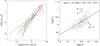 |
Fig. 1. The L − σ plane. Left panel: the L − σ plane filled by few simulated ETGs followed by the Illustris simulation from z = 4 to z = 0. Each color marks the path of a single galaxy. Right panel: observed L − σ plane. Gray dots are the ETGs with available σ in our sample. The solid line is the least square fit. The arrow shows the direction of motion for two different values of β. |
We can account for such behavior adopting the law introduced by D’Onofrio et al. (2017) to explain the tilt of the FP:
In this relation the parameter  and β (both functions of time) can vary considerably from galaxy to galaxy, assuming both positive and negative values (see Fig. 1 right panel). Each galaxy can move in this plane across time, but only in the direction fixed by β (marked by black arrows only for two possible cases).
This relation has nothing in common with the FJ law L = L0σα, where α and L0 are approximately constant. The FJ is the global distribution observed when the velocity dispersion and the luminosity of ETGs are correlated. Since all galaxies are believed to be in virial equilibrium, the FJ relation simply rewrites the VT (valid for each galaxy) using luminosity instead of mass.
The  law is also valid for any single galaxy, but it expresses the way in which σ and L vary across time. This law provides a simple way of introducing the time variable parameters
  and β, which permit one to reproduce the paths suggested by Illustris. The advantage of this approach is that we are writing a new relation that is completely independent of mass and VT, but it includes time as a hidden variable. Such a relation can therefore be coupled with the VT under the assumption that the luminosity evolution proceeds in galaxies by keeping the virial equilibrium almost constant.
We see below that the predicted change in position of a galaxy in this plane, as a consequence of evolution, has an important impact on the relations connected with the FP. Figure 2 shows the change in position for three galaxies of the Illustris simulation labeled A, B, and C, starting from z = 4 (blue dots) to z = 1 (green dots) and z = 0 (red dots), superposed to the real data (gray dots) at z = 0 for all distributions linked to the FP. Each object is followed by the simulation in its transformation across time.
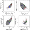 |
Fig. 2. Four projections of the FP. The small gray dots mark the observational data. The colored dots are three simulated galaxies (A, B, C) of the Illustris simulation taken along their evolution at z = 4 (blue dots), z = 1 (green dots), and z = 0 (red dots), respectively. The solid lines connect each object in its evolution with time. In this figure < Ie> is equal to Ie and indicate the average effective surface intensity. |
We note that while the L − σ relation is almost preserved in shape and scatter (only a systematic tilt toward slower slopes is observed going from z = 4 to z = 0, see D’Onofrio et al. 2020), there is a substantial difference in the appearance of all the other projections of the FP. More specifically, the distributions observed in the Ie − Re, Re − L, and Re − σ planes show a big cloud of points for the low luminous galaxies and a less scattered tail for the bright galaxies. The general impression is that two populations of galaxies fill such planes (see e.g. Capaccioli et al. 1992) and that there is a sort of “curvature” in the distributions going from one family to the other.
In general, the simulation follows the trends observed in the real data quite well (see below), reproducing, in particular, the clouds of points that formed by the faint galaxies and the tails characterizing the distribution of the brightest galaxies.
The second equation of interest is that of the VT. In the classical explanation of the FP tilt, it is implicitly assumed that a smooth variation of the zero-point of the VT equation introduces the observed tilt. The VT, in fact, can be written in its scalar form using luminosity instead of mass:
where G is the gravitational constant and kv is a term that gives the degree of structural and dynamical nonhomology4 as a function of the Sérsic index n (kv = ((73.32/(10.465 + (n − 0.94)2)) + 0.954)); see Bertin et al. 1992; D’Onofrio et al. 2008).
The combination of Eqs. (2) and (3) permits one to predict the slope and zero-point of the line along which a galaxy evolves in each projection of the FP. While the zero-point is a function of both  and β, the slope turns out to depend only on β. In other words, the motion of a galaxy in these planes is constrained by the motion that occurred in the L − σ plane. For the Ie − Re plane, we do indeed have

where
and Π is a factor that depends on kv, M/L, β, and  :
:
![$$ \begin{aligned} \Pi = \left[ \left(\frac{2\pi }{L^{\prime }_0}\right)^{1/\beta } \left(\frac{L}{M_*} \right)^{(1/2)} \left(\frac{k_{v}}{2\pi G} \right)^{(1/2)} \right]^{\frac{1}{1/2-1/\beta }}. \end{aligned} $$](/articles/aa/full_html/2022/05/aa42851-21/aa42851-21-eq21.gif)
This equation gives the only possible direction of motion of a galaxy in the Ie − Re plane as a function of β. The orientation of the motion depends on the type of transformation that a galaxy is experiencing (e.g., merging, stripping, shock, star formation, quenching, etc.).
Another combination gives the following:
that is the Re − M∗ relation. It is important to note again that the zero-point of the relation for each single galaxy depends on both  and β, while the direction of motion depends on only β.
In addition we have
for the Re − σ relation and
for the Re − L relation.
Finally we have the following:
where
for the Ie − σ relation.
Table 1 lists the slopes (i.e. the direction of evolution of a galaxy) in the various projections of the FP predicted on the basis of the values of β. We note that the values of these slopes imply a different motion for each galaxy that is associated with the variation observed in the L − σ plane.
Slopes in the FP projections.
Looking at this table in detail, we can note that: (1) In all FP projections, when β becomes progressively negative, that is to say when the objects are rapidly declining in their luminosity at nearly constant σ, the slopes either converge to the values predicted by the VT (in the Ie − Re relation and in the Re − L relation), or they diverge toward large values (in the Ie − σ and Re − σ relations), because the galaxy keeps its velocity dispersion when the luminosity decreases (only Ie and Re vary). (2) Both positive and negative values of the slopes (i.e. the direction of evolution) are permitted, which is in agreement with simulations. In general, objects still active in star formation or experiencing a merger have positive values of β, while those progressively quenching their stellar activity have increasing negative β. (3) The convergence of the slopes for progressively negative values of β naturally explains the existence of the ZoE in the Ie − Re and Re − L planes. Indeed, as β decreases, the galaxies cannot move in other directions. (4) The “curvature” of the relations (i.e. the transition from the big cloud of the small galaxies to the extremely narrow tail of the brightest objects) is naturally explained by the existence of positive and negative values of β.
The easiest way to understand the effects of all possible variations of the fundamental quantities defining the status of a galaxy is to look at the possible movements of a galaxy in the L − σ plane during its evolution (four in total). Such movements are schematically shown in Fig. 3, which displays, according to the values of β, the expected variations of Re, Ie, L, and M*, as indicated by the arrows. The figure also indicates the possible physical mechanism at the origin of the observed variations. Panels with green and blue colors correspond to positive and negative values of β, respectively. We note that when β is negative, there is not necessarily a decrease in luminosity, while when β is positive, a decrease in luminosity might also occur.
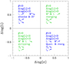 |
Fig. 3. Δlog(L)−Δlog(σ) plane. The green and blue colors mark the β > 0 and β < 0 directions of motion in the L − σ plane, respectively. Depending on the direction a galaxy experiences a change in its structural parameters and moves in the FP projections according to the slopes listed in Table 1, as described in the quadrant. |
When the luminosity of a galaxy changes, the effective radius and the mean effective surface brightness Ie both vary. This happens because Re is not a physical radius, such as the virial radius which only depends on the total mass, but it is the radius of the circle that encloses half the total luminosity of the galaxy. Since the ETGs have different stellar populations with different ages and metallicity, it is highly improbable that the decrease in luminosity does not change the whole appearance of the luminosity profile5. Consequently the growth curve changes and determines a variation of Re and Ie. If the luminosity decreases passively, in general one could expect a decrease in Re and an increase in Ie. On the other hand, if a shock induced by harassment or stripping induces an increase in L (and a small decrease in σ), we might expect an increase in Re and a decrease in Ie.
The observed variations of these parameters stongly depend on the type of event that a galaxy is experiencing (stripping, shocks, feedback, merging, etc.). In general, one should keep in mind that these three variables, L, Re, and Ie, are strongly coupled to each other and that even a small variation in L might result in ample changes in Re and Ie.
All these effects are better illustrated in Fig. 4, which shows the projections of the FP at redshift z = 0 (the present). In each panel we also visualize the direction that each galaxy would follow due to the temporal evolution of the fundamental relationship  via the parameters
  and β, and the latter in particular. The virtual displacement for negative (positive) values of β is indicated by the blue (green) arrows. Common to all panels is the striking curvature of all the relations and the existence of the ZoE in two of them that seems to correspond to large negative values of β.
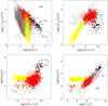 |
Fig. 4. Four different projections of the FP. The yellow dots mark the data of the Illustris simulation. The red dots are the sample with available stellar masses and velocity dispersion. The black dots are the BCG and second brightest ETGs of the clusters. The gray small dots are the optical and spectroscopic data for the objects that do not have a measured stellar mass. The dashed lines mark the region of the ZoE. The green and blue arrows mark the direction of a future evolution expected on the basis of the values of β. The green (blue) color indicates a positive (negative) value of β. |
When looking at Fig. 4, we should remember that Re does not correspond to the radius of the VT; it is proportional to, but not identical to it. Consequently in a real galaxy, L, Ie, and Re may change with time, but σ may remain constant.
Another thing to remember is that the direction of the arrows displayed in each panel visualizes the expected displacement of a generic galaxy based on the actual value of β (labeling each arrow according to the entries in Table 1). The arrows indicate the direction of motion, not the orientation of the future temporal evolution of a galaxy. Furthermore, they do not indicate the path followed by each galaxy to reach the current observed position in the diagrams.
We now describe the panels of Fig. 4 in more detail. In the Ie − Re plane, moving from left to right, β gradually changes from positive to negative values, and the slope of the associated displacement vectors gradually changes from 1 (β = 3) to −1 (β = −100), that is toward the value predicted by the VT. The cloud of points with log(Re) < 4 is likely due to a mixture of possible transformations of galaxies (with positive and negative values of β) determining different effects on Ie and Re, as a consequence of changes in luminosity. For log(Re) > 4, the tail of the bright galaxies develops, which is populated by objects that nowadays likely have negative β and consequently can move only along the direction with a slope close to −1. It is important to emphasize that the observed Ie − Re plane can only catch the situation at z = 0 as photographed by the data. Nevertheless, thanks to the effect of β on the slope of the various relations (see Table 1), we have an idea of the effect of time on the position of galaxies in this plane via the effects on L, Ie, and Re.
In this plane the ZoE is also visible with its border marked by the dashed line. The region on the right-hand side of this line is forbidden to galaxies. In the current view, this region naturally arises when the values of β become large and negative (β ≪ 0), which yield a slope for the boundary converging to −1, that is the same value expected from the VT. Galaxies that are fully dynamically relaxed and in a phase of passive evolution at decreasing luminosity are then expected to move parallel to the ZoE boundary from the side of the permitted area. We should keep in mind that the highly negative β ≪ 0 values do not fix the position of the ZoE in the diagram, but only the direction. This means that β does explain the physical reason why galaxies avoid such a region. It only demonstrates that as evolution proceeds toward the quenching of star formation and the absence of merging, galaxies can no longer move perpendicularly to the border of the ZoE and cross it. In other words, the physical origin of the ZoE should not be associated with the values of β, but with the intrinsic properties of ETGs and their halos. Along the ZoE line, ETGs seem to reach a maximum M*/L and a minimum possible radius Re for each mass and luminosity. A possible physical explanation of the origin of the ZoE is given by Chiosi et al. (2020).
The Ie − σ is a second projection of the FP. It is important to note the strong bending of the ETGs’ distribution in such a diagram. Again, the values of β predict the slopes of the corresponding displacement vectors that account for the distributions of the observational data in this plane fairly well. Clearly, the surface brightness of an object decreases when its radius increases, and it rapidly falls at nearly constant σ (see the position of the BCGs). On the other hand, when the evolution induces an increase in luminosity, the galaxies climb the relation. It is important to remember that a negative value of β does not necessarily mean a decrease in luminosity. The simulations of model galaxies at different redshifts (times) show that an increase in L is possible even when σ decreases. Such an event may likely happen, that is to say as a consequence of stripping, when some stars are removed from the galaxies, but a shock induces a new star formation event that increases the galaxy luminosity. We can also appreciate that negative values of β reproduce the tail of BCGs quite well. We also note that in this diagram, there is no clear evidence of the ZoE, in other words the values of β do not converge at a limit, as in the case of the Ie − Re relation. When β starts to be negative, the motion of the galaxies in this plane occurs along a direction opposite to that observed when β > 0.
Finally, we note that the data of the Illustris simulation for the low mass galaxies (yellow dots) largely differ from the position of real objects. Since in the Ie − Re plane the artificial galaxies have systematically larger Re, with respect to real galaxies, here their surface brightness is systematically lower. However, the tail of the BCGs is again well reproduced. The explanation could be the same as the one suggested by Chiosi et al. (2020) for the Re − M* relation, specifically for bad estimates of the energy feedback and of the presence of galactic winds.
The Re − σ plane is the third projection of the FP. The diagram has many points in common with the previous one, specifically the central bulk of ETGs (the crowed cloud), the tail that formed by the BCGs with large Re and σ characterized by β = −3.5, and the region of the faint dwarfs. The values of β in the cloud and in the region of the dwarfs might be either positive or negative. In the figure, we plotted the value of β = 1 which indicates a movement nearly orthogonal to that followed by the bright galaxies. The same remarks made above about the missing evidence of ZoE and the discrepancy between theory and data concerning the position of the low mass galaxies can be applied.
With the variables Ie and Re, we can construct another plane (the Re − L plane) which is a proxy of the well-known Re − M* plane. Luminosity is in fact mainly proportional to stellar mass (another possible source of luminosity variation, but much less important), but for the period of time with intense star forming activity, during which it is very high and changes on a short timescale, or when star formation is over and it gently and steadily decreases. Differences in chemical composition induce modest variations in the luminosity; merger episodes (unless among objects of a comparable mass) cause variations in luminosity of moderate intensity that are soon smeared by the dominant underlying stellar populations.
In general, the Illustris simulation, despite the clear failure in reproducing the radii of the fainter galaxies, is able to reproduce the curvature of the relation: faint galaxies distribute with a mean slope (about 0.3) corresponding to β ∼ 3, ETGs roughly distribute with a mean slope of 0.5 (β = 4), and finally BGCs are located in a tail with a slope ≃1 and β < 0 (approximating the same value predicted by the VT). These objects are indeed very old and do not suffer from the effects of merging and star formation anymore. They are evolving passively.
In this plane we can again identify the ZoE and its boundary along which the parameter β is high and negative, and the slope of the Re − L relations tends to 1. Notably, this is the same behavior observed in the Ie − Re plane.
In summary, what we claim here is that all of these diagrams should be analyzed taking the effects of time into account and they should not be investigated separately. They are snapshots of an evolving situation, and such temporal evolution cannot be discarded in our analysis. The  law captures such evolution in the correct way, predicting the correct direction of motion of each galaxy in its future. This way of reasoning could, in principle, allow us to determine why galaxies are in the positions we observe today in each diagram. Although β gives only the actual direction of motion and not the direction from which galaxies come (from the past), the simultaneous use of simulations and high redshift observations might help to infer the possible precursors of the present-day galaxies on the basis of the physical properties and the distribution in the FP projections, in connection with the values of β. In other words, these scaling relations become a possible tool to infer the evolutionary path of each galaxy. Since this is not the aim of the present work, but only a suggestion for a possible future line of research.
Continuing the exploration of the advantages of the VT  connection, we note a further possibility offered by the joined action of the VT and
  relation. The combination of Eqs. (4) and (6) gives an expression (very similar to that of the FP, that is to say the equation of a plane surface) that can be written as a function of β. We get the following:

where

This is valid when Ie is expressed in L⊙ pc−2 and Re is in kiloparsecs.
It should be stressed that Eq. (9) is not the FP, which is the fit of the 3D distribution of ETGs in the log(σ)−log(Ie)−log(Re) space. It shows us, however, that each single galaxy satisfies an equation similar to that of the FP (i.e. of the type log(Re) = a log(σ) + b log(⟨I⟩e) + c). This can be obtained calculating the following coefficients:


The final conversion to the measured c of the FP coefficient (being generally Re given in kiloparsecs and ⟨μ⟩e in mag arcsec−2) is then obtained from the following:

In other words, Eq. (9) indicates that in each ETG, the mass and luminosity are strongly coupled. The luminosity evolution in virialized objects does not produce a chaotic distribution in the FP projections, but it gives rise to emerging features in these diagrams (i.e. the tail of bright objects and the ZoE). The solution of the tilt problem of the FP resides in this strong coupling.
We note that in the hierarchical framework, all the FP coefficients depend on β. In addition, it is remarkable that the coefficients a, b, and d of Eq. (9) are exactly 0 when β = 2. This is due to the fact that for this exponent, the VT and the  law are the same relation. The combination of the two relations in this case has no meaning.
Conversely we can derive β from Eq. (9), being that this parameter is the only unknown one. By inverting Eq. (9), we can derive β for each of the 479 galaxies of the WINGS sample. We get the following:
which is a cubic equation in β of the type

with the following coefficients:


Such equation admits three real solutions when the discriminant Δ < 06. The mean value of the first solution from our sample of ETGs is ⟨β1⟩ = 2.78 ± 0.08, that of the second solution is ⟨β2⟩= − 2.54 ± 0.06, and that of third solution ⟨β3⟩ = 3.76 ± 0.07. It is therefore interesting to note that despite the differences in σ, Re, Ie, n, and M*/L among galaxies, the scatter around each solution is very small. As a matter of fact, the mean values of the coefficients α for the observational values of the Ie, Re, M*, kv, and σ of the 479 ETGs, are as follows:


and the uncertainties of which are not negligible. In considering the 3σ interval of a possible variation in the α values, it is indeed somewhat surprising to find three solutions for β with such a small scatter.
We can suspect that in this sample of ETGs, at variance with the large possible values of β permitted by simulations (see below), only well-defined values of β are permitted and, notably, they are both positive and negative, which is in agreement with simulations. The only possible explanation for such fine-tuned values of β is that all the ETGs considered here have had very similar histories of mass assembly. The general impression is that there are two groups of galaxies on average, one with negative values of β that are likely in a quenched state today and one with positive β, and therefore they are still active in their evolution. Notably, large negative values of β are not observed, a fact that implies that the galaxies have not yet reached the pure passive evolution, when there are no longer mergers and other disturbing effects.
Unfortunately, we cannot say which is the correct value of β for each galaxy. Nevertheless, we see below that some solutions can be discarded on the basis of the constraints imposed by the FP.
Before doing this, we performed a final test that is possible with the simulations, that is to verify the validity of Eq. (10) for the simulated objects. Such a test, however, is only possible when all the Re, Ie, n, σ, and M*/L quantities are available. The problem here is the correct estimate of Re and n. These parameters are not easy to derive from simulations, where the only data at disposal are the x, y, z positions, luminosity, and velocity of the mass particles. We estimated these parameters for a subset of 45 ETGs from the Illustris data set, reconstructing the growth curve of each object and estimating Re and n with great accuracy. The result of the test is shown in Fig. 5.
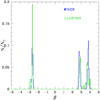 |
Fig. 5. Histogram of the calculated values of β for the WINGS and Illustris ETGs. WINGS is marked with a blue line, and Illustris is shown with a green line. |
We observe that, even in the case of simulations, three well-defined real solutions for β exist for the ETGs and they are perfectly coincident with those found for the real galaxies. The physical interpretation of this behavior is too complex to be addressed in this work, whose aim is simply to show that the mass-luminosity coupling obtained by the VT and Eq. (2) is able to account for many of the properties observed in the FP projections and to give an explanation for the tilt of the FP. Figure 6 again shows the solution we have obtained for the values of β compared with the values derived from the Illustris simulation. In this case, however, β was easily obtained by looking at the values of L and σ at two different redshift epochs:

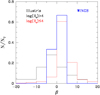 |
Fig. 6. Histogram of the calculated values of β marked with a blue line. The values of β from the Illustris simulation are shown in two histograms with black and red colors to distinguish objects with log Re > 4 and log Re ≤ 4, respectively. |
In the figure, we estimated β passing from z = 1 to z = 0. In this case, the bin of the histogram is much wider than in Fig. 5.
We note the impressive superposition of the histograms, obtained in two completely different ways, and the fact that both negative and positive values for β are admitted as solutions. The simulation, however, predicts the existence of both larger negative and larger positive values of β for few galaxies (see, D’Onofrio et al. 2020), a fact not observed in our data. This is possibly due to the fact that in the simulations, all types of objects are considered. The smaller ones in particular can be characterized by large positive and negative variations of β (star formation events, merging, big stripping of material, etc.). What is important to stress is that the large majority of the βs, predicted by the simulations, are in the same region predicted by our calculations.
Here, we provide a possible estimated error for the β solution of each single galaxy. We get the following: Δβ1 = ±0.16, Δβ2 = ±0.016, and Δβ3 = ±0.35. These uncertainties are larger than the scatter found for each β solution. They were obtained by adding the known uncertainties on σ, Re, Ie, n, and M*/L and deriving the new solutions for β. However, in some cases, when we added such uncertainty to the structural parameters, we obtained some complex solutions for β. On the contrary, when we dropped these uncertainties, we again got three real solutions for β. This fact requires a much deeper analysis of the β solutions and it is postponed to future studies. What is clear is that the possible real solutions for β require very good knowledge of the structural parameters of the galaxies. The possibility of determining β, and therefore  , for each galaxy is indeed rich of possible consequences for our study of galaxy evolution. It is also interesting to guess what values of β could be obtained for high redshift galaxies.
An important fact to stress is that knowing the solutions for β immediately leads us to determine the zero-point  on the basis of Eq. (2).
Figure 7 clearly demonstrates that the zero-point L0 of the FJ relation, which is given by the fit of the ETGs’ distribution in the L − σ plane, is simply the average value of the large number of  obtained for each galaxy. Within the errors, the average of
  and the fitted value L0 are indeed identical. It follows that the FJ relation is the average distribution, naturally resulting from the hierarchical evolution of ETGs.
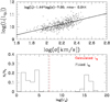 |
Fig. 7. Upper panel: FJ plane. The gray dots are the observational data and the solid black line is the least square fit. Bottom panel: histograms of the calculated values of |


The final step, shown in Fig. 8, is related to the FP coefficients. Equation (9) tells us that each galaxy follows its own FP-like equation whose coefficients are a function of β. In the figure the gray bands mark the interval of a, b, and c obtained by D’Onofrio et al. (2008), fitting the FP of ETGs separately for each cluster of the WINGS data set. The histograms mark the distribution of the coefficients a, b, and c obtained writing the FP in its classical form:

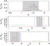 |
Fig. 8. Histograms of the values of the FP-like coefficients a, b, and c. The green, blue, and red colors correspond to the three solutions found for β, respectively. The gray band in each plot marks the region of the coefficients obtained by D’Onofrio et al. (2008) for the fit of the FP of the different WINGS clusters. The dashed black lines are the average values of the FP-like coefficients obtained considering only solutions β2 (blue) and β3 (red), and discarding solution β1 (green) which clearly does not fit with the intervals of the measured FP coefficients. |
where the units are in kiloparsecs for Re and mag arcsec−2 for ⟨μ⟩e.
The plotted solutions for the FP-like coefficients are plotted with different colors according to the values of β. Notably, we observe that the solution β1 does not fit the b and c coefficients. For this reason, we decided to discard this solution for the moment.
Again we see that the mean value of the FP-like coefficients obtained from the β2 and β3 solutions, which are all negative and positive, respectively, perfectly enters in the gray region of the permitted coefficients measured from the fit of the FP. The correct expression of the FP-like coefficients as a function of β is further secured by the fact that when β = 4, that is to say when we used the value of the FJ relation predicted by the VT, the values of the calculated coefficients of the FP as a function of β, are exactly the values predicted by the VT, that is a = 2 and b = 0.4.
In summary, we claim that, also in this case, the values of the coefficients derived from the fit of the FP are nothing else that the average value of the two possible solutions for the coefficients found for each β. Clearly, each galaxy sample under analysis will have its own number of objects with β2 and β3 values (in agreement with the evolutionary status of the sample). This naturally accounts for the small variations observed in the fits of the FP obtained from different data samples7.
It is also important to remark that, as seen in the middle and bottom panel of Fig. 8, there are no values for β that can reproduce the most accredited values for the coefficients b and c, which are ≈0.3 and ≈ − 8, respectively. This means that the measured values coming from the fit of the FP are averages of the possible coefficients for b and c. These are different from the prediction of the VT because the L − σ relation is time-dependent and it produces galaxies with both negative and positive values of β (in an unknown proportion). Consequently, each galaxy follows its own FP-like equation, which is very similar, but not equal to the FP.
In addition, the existence of different coefficients as a function of β might naturally account for the claimed bending of the FP, when we inserted the smaller ETGs in the sample. In other words, the FP is not a plane, but a surface, originating from the hierarchical evolution and the way in which mass and luminosity are coupled together.
Having demonstrated that the combination of the VT and  law is the key to interpreting the different aspects of the FP projections, we can discuss now how it is possible to account for the variation of the slope visible in the FJ relation and how it was measured by several authors. Starting from the VT,

when the luminosity is substituted to M* and Re, and one obtains the following two different trends:
These values of the slopes, which are different for high and low luminous galaxies, are in good agreement with observations (see e.g., Choi et al. 2007; Desroches et al. 2007; Hyde & Bernardi 2009; Nigoche-Netro et al. 2010; Montero-Dorta et al. 2016).
This change in slope occurs because M* scales as L1.12 over the whole mass range, while Re follows two different trends at the low and high mass ranges. In particular, we derive that Re ∝ L0.17 at the low masses and Re ∝ L0.70 at the high masses. The slopes in log units are therefore very close to that observed. Clearly, a small difference in the Re − L relation can fit the trends derived from the fits exactly.
The last thing to discuss is the origin of the small scatter that is visible in both the FJ and FP relations. In the Illustris numerical simulation, the intrinsic scatter around the FJ relation is always quite small (≈0.09), despite there being a clear rotation of the whole distribution toward a smaller slope (≈2) going from z = 4 to z = 0 (see, D’Onofrio et al. 2020). The same effect has been observed for the FP (Lu et al. 2020) with the Illustris-TNG data. As discussed in the introduction, the most accepted view is that galaxies deviate from the plane according to their M/L ratio.
In the hierarchical context, the concept of FP needs clarification. We need to remark that the FP is only the fit of a distribution. In reality, each galaxy follows its own FP-like relation, given by Eq. (9). The measured coefficients of the FP are only averages of the possible FP-like coefficients of each galaxy. Consequently, the scatter is not a well-defined concept in this case. Since there is not a unique relation that allows us to define the scatter around it, we can only try to reproduce the scatter of the FP by supposing that all galaxies have the same β. Indeed, in this case, the coefficients a1, b1, and c1 of Eq. (9) are all equal, while d1 can change for the different values of kv and M*/L. In particular, if we put β = 0.6 (the mean value of β2 and β3), the observed scatter is ≈0.068, a value very close to the measured intrinsic scatter of the FP. This means that the deviations from the FP have been correctly attributed to the nonhomology of galaxies and their different mass-to-light ratio. The small observed scatter implies only that ETGs are a very homogeneous population of galaxies, with very similar properties on average.
If the hierarchical evolution proceeds with a strong coupling of mass and luminosity, the scatter of the FP and the FJ relations, remain quite small. Only the tilt of both relations is affected by such coupling and the slope is shifted toward smaller values than those predicted by the VT. In general, we can argue that the main reason for such small scatters in the FJ and FP relations is necessarily linked to the role of gravity. Gravitation provides the dynamical relaxation of the stellar systems in short times with respect to the timescale of stellar evolution. The galaxies are always close to the virial condition. Luminosity, on the other hand, can vary in the way we have seen, but never with increments and decrements larger than a factor of 2 − 3, that is about 0.2 − 0.3 in log units. It follows that the scatter around the FJ and FP relations always remains very small, even if the luminosity variations operate the changes in the aspect of the FP projections, mostly because the luminosity variations are associated with large changes of Re and Ie.
4. Conclusions
In summary, the use of the  relation as a proxy of evolution, marking the path followed by ETGs in the L − σ plane, when combined with the equation of the VT provides the following pieces of evidence:
-
The FP can be understood as the average of the single FP-like relations that are valid for each galaxy (Eq. (9)). The coefficients of the FP-like relation are a function of β. This means that the FP must evolve with redshift and that its coefficients depend on the adopted waveband (in which observations are taken) and on the nature of the data sample (how many ETGs are included), as confirmed by the current observational data.
-
Only two of the three possible real solutions found for β, using the observations of the WINGS database and the Illustris simulation, provide the correct coefficients of the FP. Furthermore, bending the FP might naturally be explained by invoking different solutions for β.
-
The tilt of the FP results from the average values of the FP-like coefficients of Eq. (9) as a function of β.
-
The zero-point of both the FP and FJ relations is the average value of the zero-point coefficients obtained for different β.
-
All the characteristics of the FP projections can be explained at the same time. This includes the following: (1) the curvature of the relations, which turns out to depend on the existence of positive and negative values of β, and (2), the existence of the ZoE, that is the line marking the separation between the permitted and prohibited regions in these planes. No galaxies can reside in the ZoE.
-
The ZoE is obtained in a natural way as the only possible evolutionary path for objects with negative βs. These objects start to quench star formation and their luminosity progressively decreases. This corresponds to progressively smaller negative values of β, determining a saturation in the slopes permitted in the other FP projections. When the ETGs become passive quenched objects, with a luminosity decreasing at nearly constant σ, the galaxies can only move in one direction, which is dictated by the negative values of β.
We conclude noting that our empirical approach is able to explain, at least qualitatively, the problem of the tilt of the FP and the origin of all the distributions of ETGs in the FP projections. This can only be achieved by invoking the temporal evolution of galaxies and the mutual connection between mass and luminosity.
All the diagrams related to the structural parameters that are involved in the FP are sensitive to the temporal evolution of galaxies, simply because each individual object can move in a different way according to the value of β. This must happen whenever the luminosity variations occur in almost virialized objects.
The  relation is an empirical way to catch such temporal evolution. The values of β are related to the history of mass assembly and to the luminosity evolution. In the hierarchical context, in fact, the role of mass should not be confused with that of luminosity. Mass and luminosity in each galaxy can vary in different ways. For example, in the absence of merger events and as time goes by, all galaxies progressively decrease in their luminosity while keeping their mass constant.
In the hierarchical scenario, the tilt of the FP and the observed distributions of ETGs in its projections depend on the evolutionary path followed by galaxies of different masses. Only when galaxies become passive and quenched objects do they start to approach the distribution expected from the VT.
Last but not least, we mention here the result obtained by D’Onofrio & Chiosi (2020), who demonstrate that it is impossible to reproduce the Ie − Re plane starting from the L = L0σα relation and using the values of L0 and α derived from the fit of the FJ. The only way to achieve this is to allow for much larger variations of such parameters, that is to say using the  relation. For this reason, this approach also solves the old problem of connecting the L − σ and Ie − Re planes.
We are aware that the proposed scenario is not free from doubts and possible criticisms. The effective role of β needs better clarifications in the future, in particular for the measured values obtained from Eq. (10) that imply a very small range of possible solutions. This is deferred to future investigations. The only aim of this work is to stress that the simple idea of coupling mass and luminosity, that is of a simultaneous validity of the VT and Eq. (2), is able to account for many of the properties of ETGs observed in the FP projections, and it is able to explain why the FP is tilted.


We remark, however, that the large interval of the FP coefficients found by D’Onofrio et al. (2008) is also due to the small number of galaxies available for some clusters. Clusters with less than 30 objects have a large error in the measured FP slope.
Acknowledgments
The authors thank the Department of Physics and Astronomy of the Padua University for the economical support.
References
- Allanson, S. P., Hudson, M. J., Smith, R. J., & Lucey, J. R. 2009, ApJ, 702, 1275 [NASA ADS] [CrossRef] [Google Scholar]
- Auger, M. W., Treu, T., Bolton, A. S., et al. 2010, ApJ, 724, 511 [NASA ADS] [CrossRef] [Google Scholar]
- Bernardi, M., Sheth, R. K., Annis, J., et al. 2003, AJ, 125, 1866 [Google Scholar]
- Bertin, G., Saglia, R. P., & Stiavelli, M. 1992, AJ, 384, 423 [NASA ADS] [CrossRef] [Google Scholar]
- Bettoni, D., Kjærgaard, P., Milvan-Jensen, B., et al. 2016, in The Universe of Digital Sky Surveys, eds. N. R. Napolitano, G. Longo, M. Marconi, M. Paolillo, & E. Iodice, 42, 183 [NASA ADS] [CrossRef] [Google Scholar]
- Biviano, A., Moretti, A., Paccagnella, A., et al. 2017, A&A, 607, A81 [NASA ADS] [CrossRef] [EDP Sciences] [Google Scholar]
- Bolton, A. S., Burles, S., Treu, T., Koopmans, L. V. E., & Moustakas, L. A. 2007, ApJ, 665, L105 [NASA ADS] [CrossRef] [Google Scholar]
- Bolton, A. S., Treu, T., Koopmans, L. V. E., et al. 2008, ApJ, 684, 248 [NASA ADS] [CrossRef] [Google Scholar]
- Borriello, A., Salucci, P., & Danese, L. 2003, MNRAS, 341, 1109 [NASA ADS] [CrossRef] [Google Scholar]
- Busarello, G., Lanzoni, B., Capaccioli, M., et al. 1998, Mem. Soc. Astron. It., 69, 217 [NASA ADS] [Google Scholar]
- Capaccioli, M., Caon, N., & D’Onofrio, M. 1992, MNRAS, 259, 323 [NASA ADS] [CrossRef] [Google Scholar]
- Cappellari, M. 2013, ApJ, 778, L2 [NASA ADS] [CrossRef] [Google Scholar]
- Cappellari, M., Bacon, R., Bureau, M., et al. 2006, MNRAS, 366, 1126 [Google Scholar]
- Cariddi, S., D’Onofrio, M., Fasano, G., et al. 2018, A&A, 609, A133 [NASA ADS] [CrossRef] [EDP Sciences] [Google Scholar]
- Cava, A., Bettoni, D., Poggianti, B. M., et al. 2009, A&A, 495, 707 [NASA ADS] [CrossRef] [EDP Sciences] [Google Scholar]
- Chiosi, C., & Carraro, G. 2002, MNRAS, 335, 335 [NASA ADS] [CrossRef] [Google Scholar]
- Chiosi, C., Bressan, A., Portinari, L., & Tantalo, R. 1998, A&A, 339, 355 [NASA ADS] [Google Scholar]
- Chiosi, C., D’Onofrio, M., Merlin, E., Piovan, L., & Marziani, P. 2020, A&A, 643, A136 [NASA ADS] [CrossRef] [EDP Sciences] [Google Scholar]
- Choi, Y.-Y., Park, C., & Vogeley, M. S. 2007, ApJ, 658, 884 [NASA ADS] [CrossRef] [Google Scholar]
- Ciotti, L. 1991, A&A, 249, 99 [NASA ADS] [Google Scholar]
- Ciotti, L., Lanzoni, B., & Renzini, A. 1996, MNRAS, 282, 1 [Google Scholar]
- de Carvalho, R. R., & Djorgovski, S. 1992, ApJ, 389, L49 [NASA ADS] [CrossRef] [Google Scholar]
- de Graaff, A., Bezanson, R., Franx, M., et al. 2021, ApJ, 913, 103 [CrossRef] [Google Scholar]
- Desroches, L.-B., Quataert, E., Ma, C.-P., & West, A. A. 2007, MNRAS, 377, 402 [NASA ADS] [CrossRef] [Google Scholar]
- Djorgovski, S., & Davis, M. 1987, ApJ, 313, 59 [Google Scholar]
- D’Onofrio, M., & Chiosi, C. 2020, ArXiv e-prints [arXiv:2011.07315] [Google Scholar]
- D’Onofrio, M., Capaccioli, M., Zaggia, S. R., & Caon, N. 1997, MNRAS, 289, 847 [CrossRef] [Google Scholar]
- D’Onofrio, M., Valentinuzzi, T., Secco, L., Caimmi, R., & Bindoni, D. 2006, New Astron. Rev., 50, 447 [CrossRef] [Google Scholar]
- D’Onofrio, M., Fasano, G., Varela, J., et al. 2008, ApJ, 685, 875 [CrossRef] [Google Scholar]
- D’Onofrio, M., Bindoni, D., Fasano, G., et al. 2014, A&A, 572, A87 [NASA ADS] [CrossRef] [EDP Sciences] [Google Scholar]
- D’Onofrio, M., Cariddi, S., Chiosi, C., Chiosi, E., & Marziani, P. 2017, ApJ, 838, 163 [CrossRef] [Google Scholar]
- D’Onofrio, M., Chiosi, C., Sciarratta, M., & Marziani, P. 2020, A&A, 641, A94 [NASA ADS] [CrossRef] [EDP Sciences] [Google Scholar]
- Dressler, A., Lynden-Bell, D., Burstein, D., et al. 1987, ApJ, 313, 42 [Google Scholar]
- Faber, S. M., & Jackson, R. E. 1976, ApJ, 204, 668 [Google Scholar]
- Faber, S. M., Dressler, A., Davies, R. L., et al. 1987, in Nearly Normal Galaxies. From the Planck Time to the Present, 175 [Google Scholar]
- Fasano, G., Marmo, C., Varela, J., et al. 2006, A&A, 445, 805 [NASA ADS] [CrossRef] [EDP Sciences] [Google Scholar]
- Forbes, D. A., Ponman, T. J., & Brown, R. J. N. 1998, ApJ, 508, L43 [NASA ADS] [CrossRef] [Google Scholar]
- Fritz, J., Poggianti, B. M., Bettoni, D., et al. 2007, A&A, 470, 137 [NASA ADS] [CrossRef] [EDP Sciences] [Google Scholar]
- Genel, S., Vogelsberger, M., Springel, V., et al. 2014, MNRAS, 445, 175 [Google Scholar]
- Gregg, M. D. 1992, ApJ, 384, 43 [NASA ADS] [CrossRef] [Google Scholar]
- Gullieuszik, M., Poggianti, B., Fasano, G., et al. 2015, A&A, 581, A41 [NASA ADS] [CrossRef] [EDP Sciences] [Google Scholar]
- Guzman, R., Lucey, J. R., & Bower, R. G. 1993, MNRAS, 265, 731 [NASA ADS] [CrossRef] [Google Scholar]
- Holden, B. P., van der Wel, A., Kelson, D. D., Franx, M., & Illingworth, G. D. 2010, ApJ, 724, 714 [NASA ADS] [CrossRef] [Google Scholar]
- Hopkins, P. F., Cox, T. J., & Hernquist, L. 2008, ApJ, 689, 17 [NASA ADS] [CrossRef] [Google Scholar]
- Hyde, J. B., & Bernardi, M. 2009, MNRAS, 394, 1978 [NASA ADS] [CrossRef] [Google Scholar]
- Ibarra-Medel, H. J., & López-Cruz, O. 2011, Rev. Mex. Astron. Astrofis., 40, 64 [NASA ADS] [Google Scholar]
- Jorgensen, I., Franx, M., & Kjaergaard, P. 1996, MNRAS, 280, 167 [Google Scholar]
- Kormendy, J. 1977, ApJ, 218, 333 [NASA ADS] [CrossRef] [Google Scholar]
- La Barbera, F., Lopes, P. A. A., de Carvalho, R. R., de La Rosa, I. G., & Berlind, A. A. 2010, MNRAS, 408, 1361 [NASA ADS] [CrossRef] [Google Scholar]
- Lu, S., Xu, D., Wang, Y., et al. 2020, MNRAS, 492, 5930 [Google Scholar]
- Lucey, J. R., Bower, R. G., & Ellis, R. S. 1991, MNRAS, 249, 755 [NASA ADS] [Google Scholar]
- Magoulas, C., Springob, C. M., Colless, M., et al. 2012, MNRAS, 427, 245 [NASA ADS] [CrossRef] [Google Scholar]
- Montero-Dorta, A. D., Shu, Y., Bolton, A. S., Brownstein, J. R., & Weiner, B. J. 2016, MNRAS, 456, 3265 [NASA ADS] [CrossRef] [Google Scholar]
- Moretti, A., Poggianti, B. M., Fasano, G., et al. 2014, A&A, 564, A138 [NASA ADS] [CrossRef] [EDP Sciences] [Google Scholar]
- Moretti, A., Gullieuszik, M., Poggianti, B., et al. 2017, A&A, 599, A81 [NASA ADS] [CrossRef] [EDP Sciences] [Google Scholar]
- Nelson, D., Pillepich, A., Genel, S., et al. 2015, Astron. Comput., 13, 12 [Google Scholar]
- Nigoche-Netro, A., Aguerri, J. A. L., Lagos, P., et al. 2010, A&A, 516, A96 [NASA ADS] [CrossRef] [EDP Sciences] [Google Scholar]
- Nipoti, C., Londrillo, P., & Ciotti, L. 2003, MNRAS, 342, 501 [Google Scholar]
- Novak, G. S. 2008, PhD Thesis, University of California, Santa Cruz [Google Scholar]
- Pignatelli, E., Fasano, G., & Cassata, P. 2006, A&A, 446, 373 [NASA ADS] [CrossRef] [EDP Sciences] [Google Scholar]
- Prugniel, P., & Simien, F. 1997, A&A, 321, 111 [NASA ADS] [Google Scholar]
- Reda, F. M., Forbes, D. A., & Hau, G. K. T. 2005, MNRAS, 360, 693 [NASA ADS] [CrossRef] [Google Scholar]
- Renzini, A., & Ciotti, L. 1993, ApJ, 416, L49 [NASA ADS] [CrossRef] [Google Scholar]
- Robertson, B., Cox, T. J., Hernquist, L., et al. 2006, ApJ, 641, 21 [NASA ADS] [CrossRef] [Google Scholar]
- Samir, R. M., Reda, F. M., Shaker, A. A., Osman, A. M. I., & Amin, M. Y. 2016, NRIAG J. Astron. Geophys., 5, 277 [NASA ADS] [CrossRef] [Google Scholar]
- Strauss, M. A., & Willick, J. A. 1995, Phys. Rep., 261, 271 [NASA ADS] [CrossRef] [Google Scholar]
- Taranu, D., Dubinski, J., & Yee, H. K. C. 2015, ApJ, 803, 78 [Google Scholar]
- Tortora, C., Napolitano, N. R., Romanowsky, A. J., Capaccioli, M., & Covone, G. 2009, MNRAS, 396, 1132 [NASA ADS] [CrossRef] [Google Scholar]
- Trujillo, I., Burkert, A., & Bell, E. F. 2004, ApJ, 600, L39 [Google Scholar]
- Valentinuzzi, T., Woods, D., Fasano, G., et al. 2009, A&A, 501, 851 [NASA ADS] [CrossRef] [EDP Sciences] [Google Scholar]
- van Dokkum, P. G., & Franx, M. 1996, MNRAS, 281, 985 [NASA ADS] [CrossRef] [Google Scholar]
- van Dokkum, P. G., & van der Marel, R. P. 2007, ApJ, 655, 30 [NASA ADS] [CrossRef] [Google Scholar]
- Varela, J., D’Onofrio, M., Marmo, C., et al. 2009, A&A, 497, 667 [NASA ADS] [CrossRef] [EDP Sciences] [Google Scholar]
- Vogelsberger, M., Genel, S., Springel, V., et al. 2014, Nature, 509, 177 [Google Scholar]
- Willick, J. A., Courteau, S., Faber, S. M., Burstein, D., & Dekel, A. 1995, ApJ, 446, 12 [NASA ADS] [CrossRef] [Google Scholar]
All Tables
All Figures
|
Fig. 1. The L − σ plane. Left panel: the L − σ plane filled by few simulated ETGs followed by the Illustris simulation from z = 4 to z = 0. Each color marks the path of a single galaxy. Right panel: observed L − σ plane. Gray dots are the ETGs with available σ in our sample. The solid line is the least square fit. The arrow shows the direction of motion for two different values of β. |
| In the text | |
|
Fig. 2. Four projections of the FP. The small gray dots mark the observational data. The colored dots are three simulated galaxies (A, B, C) of the Illustris simulation taken along their evolution at z = 4 (blue dots), z = 1 (green dots), and z = 0 (red dots), respectively. The solid lines connect each object in its evolution with time. In this figure < Ie> is equal to Ie and indicate the average effective surface intensity. |
| In the text | |
|
Fig. 3. Δlog(L)−Δlog(σ) plane. The green and blue colors mark the β > 0 and β < 0 directions of motion in the L − σ plane, respectively. Depending on the direction a galaxy experiences a change in its structural parameters and moves in the FP projections according to the slopes listed in Table 1, as described in the quadrant. |
| In the text | |
|
Fig. 4. Four different projections of the FP. The yellow dots mark the data of the Illustris simulation. The red dots are the sample with available stellar masses and velocity dispersion. The black dots are the BCG and second brightest ETGs of the clusters. The gray small dots are the optical and spectroscopic data for the objects that do not have a measured stellar mass. The dashed lines mark the region of the ZoE. The green and blue arrows mark the direction of a future evolution expected on the basis of the values of β. The green (blue) color indicates a positive (negative) value of β. |
| In the text | |
|
Fig. 5. Histogram of the calculated values of β for the WINGS and Illustris ETGs. WINGS is marked with a blue line, and Illustris is shown with a green line. |
| In the text | |
|
Fig. 6. Histogram of the calculated values of β marked with a blue line. The values of β from the Illustris simulation are shown in two histograms with black and red colors to distinguish objects with log Re > 4 and log Re ≤ 4, respectively. |
| In the text | |
|
Fig. 7. Upper panel: FJ plane. The gray dots are the observational data and the solid black line is the least square fit. Bottom panel: histograms of the calculated values of |
| In the text | |
|
Fig. 8. Histograms of the values of the FP-like coefficients a, b, and c. The green, blue, and red colors correspond to the three solutions found for β, respectively. The gray band in each plot marks the region of the coefficients obtained by D’Onofrio et al. (2008) for the fit of the FP of the different WINGS clusters. The dashed black lines are the average values of the FP-like coefficients obtained considering only solutions β2 (blue) and β3 (red), and discarding solution β1 (green) which clearly does not fit with the intervals of the measured FP coefficients. |
| In the text | |
Current usage metrics show cumulative count of Article Views (full-text article views including HTML views, PDF and ePub downloads, according to the available data) and Abstracts Views on Vision4Press platform.
Data correspond to usage on the plateform after 2015. The current usage metrics is available 48-96 hours after online publication and is updated daily on week days.
Initial download of the metrics may take a while.