| Issue |
A&A
Volume 661, May 2022
|
|
|---|---|---|
| Article Number | A128 | |
| Number of page(s) | 13 | |
| Section | Interstellar and circumstellar matter | |
| DOI | https://doi.org/10.1051/0004-6361/202142747 | |
| Published online | 24 May 2022 | |
Spectral softening in core-collapse supernova remnant expanding inside wind-blown bubble★
1
Deutsches Elektronen-Synchrotron DESY,
Platanenallee 6,
15738
Zeuthen,
Germany
e-mail: This email address is being protected from spambots. You need JavaScript enabled to view it.
2
Institute of Physics and Astronomy, University of Potsdam,
14476
Potsdam,
Germany
3
Dublin Institute for Advanced Studies,
31 Fitzwilliam Place,
Dublin 2
Ireland
4
Centre for Space Research, North-West University,
2520
Potchefstroom,
South Africa
5
Astronomical Observatory of Ivan Franko National University of L’viv,
vul. Kyryla i Methodia, 8,
L’viv
79005,
Ukraine
Received:
22
November
2021
Accepted:
2
March
2022
Abstract
Context. Galactic cosmic rays (CRs) are widely assumed to arise from diffusive shock acceleration, specifically at shocks in supernova remnants (SNRs). These shocks expand in a complex environment, particularly in the core-collapse scenario as these SNRs evolve inside the wind-blown bubbles created by their progenitor stars. The CRs at core-collapse SNRs may carry spectral signatures of that complexity.
Aims. We study particle acceleration in the core-collapse SNR of a progenitor with an initial mass of 60 M⊙ and realistic stellar evolution. The SNR shock interacts with discontinuities inside the wind-blown bubble and generates several transmitted and reflected shocks. We analyse their impact on particle spectra and the resulting emission from the remnant.
Methods. To model the particle acceleration at the forward shock of a SNR expanding inside a wind bubble, we initially simulated the evolution of the pre-supernova circumstellar medium (CSM) by solving the hydrodynamic equations for the entire lifetime of the progenitor star. As the large-scale magnetic field, we considered parameterised circumstellar magnetic field with passive field transport. We then solved the hydrodynamic equations for the evolution of a SNR inside the pre-supernova CSM simultaneously with the transport equation for CRs in test-particle approximation and with the induction equation for the magnetohydrodynamics in 1D spherical symmetry.
Results. The evolution of a core-collapse SNR inside a complex wind-blown bubble modifies the spectra of both the particles and their emission on account of several factors including density fluctuations, temperature variations, and the magnetic field configuration. We find softer particle spectra with spectral indices close to 2.5 during shock propagation inside the shocked wind, and this softness persists at later evolutionary stages. Further, our calculated total production spectrum released into the interstellar medium demonstrates spectral consistency at high energy (HE) with the injection spectrum of Galactic CRs, which is required in propagation models. The magnetic field structure effectively influences the emission morphology of SNRs as it governs the transportation of particles and the synchrotron emissivity. There is rarely a full correspondence of the intensity morphology in the radio, X-ray, and gamma-ray bands.
Key words: ISM: supernova remnants / ISM: bubbles / cosmic rays
Movie associated to Fig. B.1 is only available at https://www.aanda.org
© ESO 2022
1 Introduction
Supernova remnants (SNRs) are major sources of Galactic cosmic rays (CRs) below the “knee” energy (≈1015 eV) (Baade & Zwicky 1934; Blasi 2013). The acceleration mechanism able to accelerate CRs to this high energy (HE) is thought to be the widely studied diffusive shock acceleration (DSA) process (Fermi 1949; Bell 1978; Drury 1983) and its non-linear modification (Ellison et al. 1997). According to DSA, the spectra of particles accelerated during a SNR shock should follow a power law in energy with the spectral index 2, with an exponential cutoff at the maximum achievable energy, limited spatially by the size, temporally by the age of the SNR, and also by radiative energy losses and adiabatic cooling. In recent years, observations in the TeV band (surveys such as HESS, VERITAS, MAGIC, HAWC, and LHAASO) and in the GeV band (AGILE and Fermi-LAT) have been collecting a significant amount of data regarding SNRs, providing crucial insight and constraints for theoretical models. Spectral measurements of gamma-ray emission from for example IC443 (Acciari et al. 2009), Cas A (Abdo et al. 2010), SN 1006 (Acero et al. 2010), the Tycho SNR (Acciari et al. 2011), and W44 (Malkov et al. 2011; Cardillo et al. 2014) indicate a considerable softening compared to the expected power-law index s = 2, which may be modelled in different ways. For example, diffusive re-acceleration of Galactic CRs has been proposed to explain the spectral shape of W44 (Cardillo et al. 2016), but was found implausible in other studies on account of the large thickness of radiative shocks and the paucity of Galactic CRs to be re-accelerated (Brose et al. 2020; de Oña Wilhelmi et al. 2020). Other options include re-acceleration in fast-mode turbulence downstream of the forward shock (FS, Pohl et al. 2015; Wilhelm et al. 2020), fast motion of downstream turbulence (Caprioli et al. 2020), and inefficient particle confinement in the vicinity of the SNR caused by the attenuation or weak driving of Alfvén waves (Malkov et al. 2011; Celli et al. 2019; Brose et al. 2020).
The CR acceleration at SNR shocks depends on the type of the SNR and the hydrodynamic and magnetic-field structure of its environment. Specifically, the type of the progenitor star is encoded in the morphology of the core-collapse SNR (e.g. Chevalier & Liang 1989; Ciotti & D’Ercole 1989; Dwarkadas 2005, 2007; Meyer et al. 2021); for instance an “ear”-like morphology is seen for luminous blue variable (LBV) progenitors (Chiotellis et al. 2021; Ustamujic et al. 2021). CR acceleration at shocks propagating through stellar wind was discussed by Voelk & Biermann (1988), Berezinskii & Ptuskin (1989), and Berezhko & Völk (2000) considering Bohm diffusion of energetic particles. Changes in the particle spectra in the core-collapse scenario with red super giant (RSG) and Wolf-Rayet (WR) star progenitors were investigated by Telezhinsky et al. (2013) for simplified flow profiles. Most recently, the effects of the circumstellar magnetic field on electron spectra and sequent non-thermal emissions were studied by Sushch et al. (2022), focusing on the impact originating during the transition of a SNR FS from the free wind to the shocked wind region of the wind bubble. In both of these latter studies, the complete hydrodynamic evolution of the circumstellar medium (CSM) during stellar evolution was not taken into account. Nevertheless, a realistic representation of the CSM at the pre-supernova stage can potentially impose better constraints than the ones already demonstrated. Sushch et al. (2022) also investigated the impact of a parametrised postshock magnetic field amplification on the synchrotron cooling. In addition to possibly amplifying the magnetic field, resonant and non-resonant streaming instabilities determine the spectrum of turbulence, and hence the diffusion coefficient as well as the maximally attainable particle energy at any point in time during the evolution of the remnant (Brose et al. 2020). A detailed consideration of turbulent magnetic field is beyond the scope of this study. A forthcoming study including magnetic field amplification with realistic hydrodynamics shall explore the additional impact of CR-driven instabilities on particle acceleration as well as radiation from the remnant.
In this paper, we investigate the modification of spectra from CRs accelerated at the FS of an SNR as it evolves through the different regions of the wind bubble, simulated using an evolutionary track for a zero age main sequence (ZAMS) mass of 60M⊙. We present the imprint of interactions of SNR FS with multiple shocks and contact discontinuities inside the wind bubble on the particle spectra and demonstrate that the obtained CR spectra are softer than predicted for strong shocks. Additionally, we illustrate the effects of the circumstellar magnetic field along with the hydrodynamics. Although not a frequent event (Jennings et al. 2014), studying an SNR with a 60 M⊙ progenitor is interesting because emissions from the SNR with this massive progenitor star can be predicted theoretically. Furthermore, a 60 M⊙ star is thought to evolve through an LBV phase instead of an RSG phase, and ends its life as a WR star. These different evolutionary phases of this star leave imprints in the morphology of the ambient medium, and hence on the particle spectra.
2 Numerical methods
We introduce the reader to the numerical methods used in this study. The DSA at SNR FS has been modelled in test-particle approximation. The necessary constituents for this modelling are a hydrodynamic description of the CSM structure, a large-scale magnetic field profile, a prescription for diffusion, and finally the solution for the CR transport equation. We numerically solved the particle acceleration and hydrodynamics, respectively, with RATPaC (Radiation Acceleration Transport Parallel Code, Telezhinsky et al. 2012a, 2013; Brose et al. 2020; Sushch et al. 2022) and the PLUTO code (Mignone et al. 2007; Vaidya et al. 2018).
This section begins by presenting the hydrodynamics of pre-supernova CSM in which we have inserted a supernova explosion. We then describe the structure of magnetic field followed by our method for calculating the particle acceleration.
2.1 Hydrodynamics
The Euler hydrodynamic equations including an energy sourcesink term can be expressed as (considering the magnetic field too weak to be dynamically important):
 (1)
(1)
 (2)
(2)
where ρ, u, m, P, E, and S are the mass density, velocity, momentum density, thermal pressure, total energy density, and the source-sink term, respectively. I is the unit tensor.
2.1.1 Construction of CSM at the pre-supernova stage
To simulate the wind bubble created by a non-rotating 60 M⊙ star at solar metallicity (Z = 0.014) from ZAMS to the pre-supernova stage, we performed a hydrodynamic simulation with PLUTO in 1D spherical symmetry. For the simulation, the computational domain [O, Rmax] with origin O and Rmax = 150 parsec was discretised into 50000 equally spaced grid points. The interstellar medium (ISM) is assumed to have a constant number density, nISM = 1 atom cm−3. To initialise the simulation, a radially symmetric spherical supersonic stellar wind was injected into a small spherical region of radius 0.06 pc at the origin using the stellar evolutionary track for 60 M⊙ ZAMS described in Groh et al. (2014). The wind density, ρwind, can be written as:
 (3)
(3)
where r is the radial coordinate, and Ṁ and uwind represent the time-dependent mass-loss rate and the wind velocity, respectively, taken from Groh et al. (2014). To model the evolution of the wind bubble, we integrated Eqs. (1) and (2) with a second- order Runge-Kutta method, using the Harten-Lax-Van Leer approximate Riemann Solver (hll) and finite volume methodology. Further, optically thin cooling and radiative heating were included through the source-sink term, S = Φ(T, ρ), using the cooling and heating laws described in Meyer et al. (2020, Sect. 2.3). The time-steps for the simulation were constrained using the standard Courant-Friedrich-Levy (CFL) condition, initialised as Ccfl = 0.1.
The stellar evolution was followed from zero age to the presupernova phase at 3.95 million yr. The state of the CSM at this time is the initial state of the SNR simulation. Therefore, this model is a 1D equivalent of the 2D simulation in the staticstar scenario presented in Meyer et al. (2020). The stellar wind parameters at the post-main sequence stages are illustrated in Meyer et al. (2020, Sect. 2.4).
2.1.2 Modelling of the supernova ejecta profile
The density distribution of supernova ejecta is modelled as a constant, pc, up to rc, followed by a power law to the ejecta radius, Rej:
 (4)
(4)
where n = 9 is conventionally used for the core-collapse explosion. The velocity profile for the ejecta reflects homologous expansion:
 (5)
(5)
where TSN = 3 yr is the start time of the hydrodynamic simulation. The initial ejecta temperature is set to 104 K.
The expressions for rc and ρc can be written as a function of the ejecta mass, Mej, and explosion energy, Eej,
 (6)
(6)
 (7)
(7)
In our simulation, Rej = xrc and x = 2.5, Eej = 1051 erg, and Mej = 11.75 M⊙1, respectively.
2.1.3 Hydrodynamic modelling to study SNR shock evolution
To initiate the supernova explosion, the supernova ejecta profile has been inserted into, and interpolated with, the pre-calculated pre-supernova CSM profile, as illustrated in Fig. 1. To model the evolution of the SNR, we then solved Eqs. (1) and (2) considering the local source as zero (S = 0) using a Harten-Lax-Van Leer approximate Riemann Solver that restores with the middle contact discontinuity (hllc), finite-volume methodology, and a second-order Runge-Kutta method. The numerical simulation with the PLUTO code was performed in 1D spherical symmetry with 262 144 uniform grid cells with Rmax = 112 pc to provide a spatial resolution of about 0.0004 pc2.
2.2 Magnetic field
2.2.1 Field profile
To acquire the large-scale magnetic field profile for the entire lifetime of the SNR, we solved the induction equation for ideal magnetohydrodynamics (MHD) following Telezhinsky et al. (2013). This method mimics MHD for negligible magnetic pressure. The structure of the CSM magnetic field is quite intricate, specifically in the presence of the different evolutionary stages of the massive star (see for a rotating O star Mackey et al. 2020). Therefore, modelling the CSM magnetic field with the MHD simulation for the entire lifetime of the 60 M⊙ star is out of the scope of this paper, but for simplicity, we can parametrise the CSM magnetic field using background information about the stellar magnetic field.
The wind of a rotating star carries away mass and magnetic field. In the presence of a weak magnetic field, the flow speed is as for a non-magnetic wind, and the magnetic field becomes frozen-in (Cassinelli 1991). Gauss’ law (∇ B = 0) gives the expression for radial field,
 (8)
(8)
For a rotating star, the toroidal field in the equatorial plane of rotation (Ignace et al. 1998) can be written as (García-Segura et al. 1999; Chevalier & Luo 1994),
 (9)
(9)
where B⋆ and R⋆ are the stellar surface magnetic field and radius, respectively, urot and uwind represent the surface rotational velocity in the equatorial plane and the radial wind speed, respectively. The toroidal field will be strongly dominant except for very close to the stellar surface. The radial field can be expected to provide an impact only during the first days of the SNR evolution discussed in Inoue et al. (2021), and is therefore beyond the scope of this paper.
Using the wind profiles of a non-rotating 60 M⊙ star and the rotation of the WR star, the pre-supernova stage of a 60 M⊙ star, we parametrised the circumstellar magnetic field, BCSM. The surface magnetic field and stellar radius were set to 1000 Gand 6 R⊙, respectively, following Crowther (2007). The wind speed and surface rotational velocity were approximated to 2000km s−1 and 100km s−1, respectively, following Ignace et al. (1996), and Chené & St-Louis (2010). The magnetic field is compressed by a factor 4 at the wind termination shock, as is the density. For simplicity, we considered a constant field strength in the shocked wind, as a significantly more realistic model would require MHD simulations and assumptions about the magnetic field at the launch point of the stellar wind throughout the entire evolution of the progenitor star. Therefore, the magnetic field in the regions marked in Fig. 1 can be approximated as,
 (10)
(10)
For region 4, magnetic field (Bshell) has been calculated as in van Marle et al. (2015),
 (11)
(11)
where BISM is the ISM magnetic field, and R and d are the outer radius and the thickness of region 4, respectively. The magnetic field in the free wind is too weak to make the magnetic pressure dynamically important. The strength of BISM is chosen to provide super-Alfvénic motion of the shell in region 4 into the ISM, meaning we allow for an outer shock in the ISM.
For the initial magnetic field in the supernova ejecta, Bej (r) α 1/r2 satisfies ∇ Bej = 0 and ∇ × (uej × Bej) = 0 for both the radial and the toroidal field components. The normalisation is chosen to provide a volume-averaged magnetic field of 30 G when the SNR radius is 1015 cm (explained elaborately in Telezhinsky et al. 2013, Sect. 3),
 (12)
(12)
where Rsh, t0 are the SNR shock radius and starting time of simulation, respectively.
The sequent evolution is that of frozen-in magnetic field and given by the induction equation in 1D spherical symmetry (Telezhinsky et al. 2013),
 (13)
(13)
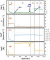 |
Fig. 1 Profiles of the number density (n, panel a), the flow speed (u, panel b), the thermal pressure (P, panel c), and the temperature (T, panel d) immediately after the supernova explosion. Vertical grey lines mark the boundary of the supernova ejecta (up to 0.023 parsec), the free stellar wind (region 1), the shocked LBV and WR wind (region 2), the shocked wind from the O and B phases (region 3), the shocked ISM (region 4), and the ambient ISM (region 5). RWT is the radius of the wind termination shock, LBV shell denotes the dense shell created by interaction between LBV wind and WR wind, and CD represents the contact discontinuity between shocked wind and shocked ISM. |
2.2.2 Diffusion coefficient
The diffusion coefficient directly influences the acceleration timescale and the maximum attainable energy of the particles (Lagage & Cesarsky 1983; Schure et al. 2010). The spatial diffusion coefficient can be expressed as,
 (14)
(14)
where ζ is a free scaling parameter and D0 is the diffusion coefficient for the nominal momentum and magnetic-field strength, either DB for Bohm diffusion with a = 1 or DG = 1029 cm2 s-1 with = 1/3 for Galactic diffusion, respectively. We applied ten times the Bohm diffusion coefficient (ζD0 = 10DB) in the entire region downstream of the SNR FS, as well as the galactic diffusion coefficient (ζD0 = DG) in the far-upstream region starting from 2Rsh (Telezhinsky et al. 2012b), and a connecting exponential profile between these two regions.
A more realistic approach would be to solve the transport equation of magnetic turbulence at least for the resonant CR streaming instability. A forthcoming study will include the magnetic field fluctuations through the diffusion coefficient prescribed in Brose et al. (2016).
2.3 Particle acceleration
The time-dependent transport equation for the differential number density of CRs, N(p), can be expressed as
 (15)
(15)
where D is the spatial diffusion coefficient, ṗ corresponds to the energy loss rate (synchrotron losses and inverse Compton (IC) losses for electrons), u refers to the plasma velocity, and Q represents the source term.
This transport equation has been solved in test-particle approximation and for spherical symmetry with RATPaC, applying implicit finite-difference algorithms implemented in the FiPy package (Guyer et al. 2009). In our simulation, the cosmic-ray pressure always remains below 10% of the shock ram pressure (Kang & Ryu 2010). We used a shock-centred coordinate system, x = r/Rsh, where Rsh is the shock radius. Additionally, we transformed the radial coordinate as (x−1) = (x*−1)3 to get a better spatial resolution near the shock, Δr/Rsh ≈ 10−6. This choice also provides a grid extent to 65Rsh to track the particles escaped from the vicinity of the shock but still inside the far upstream region.
2.4 Injection of particles
The source term in the transport equation is defined by,
 (16)
(16)
where η is the injection efficiency, and nu and uu are the upstream plasma number density and velocity, respectively, Vsh and Rsh are the shock velocity and radius, respectively, and pinj represents the momentum of injected particles. Following Blasi et al. (2005), the injection momentum is defined as a multiple of thermal momentum, pinj = ξpth =  . The injection efficiency is
 (17)
(17)
where η represents the compression ratio of the shock. The momentum of the injected particles should be significantly larger than the thermal momentum of downstream particles to participate in shock acceleration. Although Simpson et al. (2016) demonstrated that CR-feedback has an important effect on driving the galactic outflows in ISM when CRs escape the SNR at the late evolutionary stage, CR-feedback is beyond the scope of this paper. Therefore, even though ξ = 4.24 has been found appropriate for SN1006 (Brose et al. 2021, Appendix A) for example, we take ξ = 4.4, as for smaller values of ξ the test-particle approximation would not be valid when the shock passes through the dense LBV shell and through the shocked ISM. The coupled equations for the hydrodynamic evolution of the SNR, the evolution of the large-scale magnetic field, and the transport of CRs were solved simultaneously. The CR transport equation and the induction equation for the magnetic field can be solved with a time-step of 1 yr, but the standard CFL condition limits the time-step of the hydrodynamic simulation to 10−3−10−4 yr.
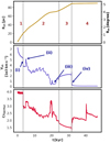 |
Fig. 2 Behaviour of FS parameters: radius (Rsh), velocity (Vsh), and shock compression ratio (CrRATPaC). In the upper panel, we also provide the angular scale, θsh, for a distance of 1000 parsec. (i)-(iv) mark interactions of the FS with different discontinuities, namely (i) the wind termination shock, (ii) another outgoing shock, (iii) the LBV shell, and (iv) the CD. |
3 Results
3.1 Shock parameters
The evolution of the SNR with a ZAMS mass 60 M⊙ progenitor was studied for 46 000 yr, until the SNR FS begins to expand inside the shocked ISM region, and the sonic Mach number of the FS falls below 2. Figure 2 illustrates the time evolution of the shock radius and velocity, as well as the shock compression ratio, as the SNR FS propagates through the various regions of the wind bubble depicted in Fig. 1. In the free stellar wind, the shock velocity gradually decreases from approximately 7300 km s−1 to 5300km s−1. After about 3300 yr, the FS interacts with the wind termination shock, transits to the denser shocked wind, and the shock speed plummets to 1500 km s−1. sequently, after nearly 4830 yr, the FS velocity rises steeply by 1400 km s−1 as a consequence of a tail-on collision between the FS and the reflection off the contact discontinuity between FS and the reverse shock (RS) of the reflected shock produced during the interaction between the FS and the wind termination shock. After that, the shock velocity fluctuates a lot, on account of interactions between the FS and various weaker discontinuities in the shocked wind. Between 19 000 yr and 23 000 yr, the FS passes through the LBV shell, followed by a slight rise in shock velocity after 24 000 yr during the passage through the low-density shocked wind of the O and B phase of the progenitor. Finally, after 32 000 yr, the FS interacts with the CD of the CSM, and the shock speed sharply falls from approximately 2000 km s−1 to 46km s−1.
In the free stellar wind, the shock is strong and the shock compression ratio is close to 4. Figure 2 demonstrates that the compression ratio falls to 2.9, as soon as the FS enters the hot shocked stellar wind, and it finally becomes 1.5 right before the FS-CD interaction at 32 000 yr. The variations in the shock compression ratio simply reflect the change in sonic Mach number of the FS, Ms. Tests verify that the numerically derived value CrRATPaC = vu/vd, with vu and vd as the upstream and downstream flow speed in the FS rest frame, conforms well with the theoretical value based on the upstream temperature and the shock speed, CrTheoretical = (1 + γ)Ms2/((γ–1)Ms2 + 2), where γ = 5/3. The shocked wind is hot enough to reduce the sonic Mach number to single-digit numbers.
3.2 Particle spectra
To evaluate proton and electron spectra at times characteristic for FS propagation through the different regions of the wind bubble, we show their volume averages for the entire region downstream of the FS. The large-scale transported magnetic field described in Sect. 2.2.1 shapes in particular the electron spectra through the synchrotron energy losses. Below a few tens of TeV, their importance relative to IC losses (cosmic microwave background (CMB) photons only) scales with the energy density ratio of magnetic field and CMB photons, UB/UCMB. In our modelled magnetic field scenario, the magnetic field inside the RS is as weak as 0.01 µG, which renders IC losses dominant in the deep interior of the SNR.
FS in the free wind
At 3000 yr the FS still propagates through the free wind and is about to interact with the wind termination shock that is located at a radius of about 20 parsec. The first and third rows of the first column of Fig. 3 show the profiles of the gas number density, n, and the magnetic field (B) respectively. The magnetic field, B, has its peak strength at the contact discontinuity between FS and RS at a radius of approximately 16 parsec, and becomes moderately weaker towards the FS. At this time, the proton spectrum reflects the E−2 expected for test-particle DSA for strong shock, and further the maximum achievable proton energy reaches 5 TeV.
FS in the shocked wind
At 4820 yr, the FS propagates through the shocked wind. A shown in the second column of Fig. 3, the proton spectrum starts to become softer than the standard power law, E−2, as a consequence of the lower sonic Mach number of the FS in this region. Also, the spectra display a convex curvature. Detailed inspection of the spatial distribution of particles reveals that the numerous transmitted and reflected shocks between the FS and the RS, which were originally spawned by the interaction between the FS and the wind termination shock, provide re-acceleration of the CRs that are primarily produced at the FS of the SNR. Any time a shock hits a discontinuity, it breaks into a transmitted shock and a reflected shock, and after a few interactions many shocks are generated.
Each of them can accelerate particles with a certain spectral index and a specific maximum energy. At high energies, the contribution with the hardest spectrum should dominate (Brecher & Burbidge 1972; Büsching et al. 2001), provided the energy can be reached, and so we see a complex superposition of the acceleration yield of many shocks. Additionally, the magnetic field downstream of the FS is very weak, and hence the diffusion coefficient is large. Therefore, sufficiently highly energetic particles can deeply penetrate the downstream region and are able to interact with some of the reflected shocks. This produces a weak but noticeable spectral break above 10 GeV. The exact form of the spectral break may depend on the details of the magnetic-field structure, implying it could be slightly different for a full MHD model or the inclusion of a grid turbulence model. This spectral break is also visible in the electron spectra at the same time, which we show in Fig. 6. Furthermore, an outgoing shock emerging from the interaction between a reflected shock and the contact discontinuity is about to collide with the FS. Only a few years later, at 4836 yr, both the shock speed and the shock compression ratio increase sharply. The third column of Fig. 3 shows the spectrum and the related parameters immediately after the shock-shock tail-on collision, and no visible change is observed in the spectrum. It appears that here shock merging does not immediately change the spectral shape of the volume-averaged proton spectrum, which also have been expected from the calculations shown in Appendix A. However, this interaction will increase the acceleration rate, and also therefore the acceleration efficiency of the FS, which eventually leads to a higher maximum energy of the particles, as also discussed by Sushch et al. (2022, Sect. 4.2). This finding is in line with recent analyses of the spectral effects of shock-shock collisions (Vieu et al. 2020). Generally speaking, the time period during which particles can see both shocks is shorter than the acceleration time.
The first column of Fig. 4 illustrates the state after 9500 yr. The FS has already gone through several interactions with different discontinuities inside the shocked stellar wind. At this time, the proton spectra are generally soft with an index of around 2.3 with moderate variations between the GeV band and about 10 TeV energies. The running spectral index at this time is also shown in Fig. 5. Later, after 28 000 yr, the FS enters the shocked wind from the O and B phases of the progenitor after crossing the LBV shell. During the passage through the LBV shell, the FS encounters a relatively dense and cold material. Consequently, the injection rate of low-energy particles into the DSA is high and the injection momentum is low because of the low shock speed. The spectra in the second column of Fig. 4 show the pile-up at very low energy that results from this amplified injection. Here, the low-energy pile-up around 10 MeV reflects the simplified injection model we used. However, the softness of the spectrum above a few tens of MeV is generic and arises entirely from the small compression ratio of the FS. The spectral index for protons reaches approximately 2.5 at energies beyond 10 GeV, as shown in Fig. 5.
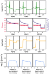 |
Fig. 3 Proton spectra volume-averaged downstream of the FS at early times: for context, we also provide the gas number density, n, as a function of radius. The second row displays the compression ratio (CrRATPaC) and the shock speed (Vsh) up to the specific age, the third row depicts the magnetic-field profile (B), and the fourth row illustrates the proton spectra. The vertical lines in the first and the third row mark the FS position. |
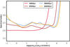 |
Fig. 5 Variation of the spectral index for protons at different ages with momentum of SNR. |
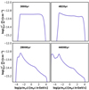 |
Fig. 6 Electron spectra at different ages of the SNR, volume-averaged downstream of the FS. |
FS in the shocked ISM
The shocked ISM is 10 000 times denser than the shocked O, B wind. Therefore, the collision between the FS and the wind-bubble CD significantly lowers the acceleration efficiency of the FS, but increases the injection rate, and leads to the formation of a reflected shock with a speed of approximately 2000 km s−1. Therefore, the FS becomes too weak to provide efficient acceleration but the reflected shock will eventually interact with other structures and will provide several outgoing shocks which can catch up to the FS at later times. The innermost reflected shock speed increases to approximately 3000 km s−1 during its propagation towards the ejecta, and it may re-energise the particles during its passage towards the interior of the remnant. This situation is similar to the efficient acceleration at the reverse shock of a very young SNR; for example Cas A (Borkowski et al. 1996). However, efficient particle acceleration at the reverse shock requires significant magnetic amplification because of the weak field in the ejecta (Ellison et al. 2005; Zirakashvili et al. 2014). After 44 000 yr, the proton spectrum, which is shown in the third column of Fig. 4, and likewise the electron spectrum illustrated in Fig. 6 are much softer than a E−2 power law. The FS propagates through a dense and cold medium, and so a huge number of low-energy particles are injected at low momenta, but the compression ratio of the FS is around 2.5. Beyond this time, we see no further change in the proton or electron spectra, and our simulation ends after 46 000 yr.
With time, the hydrodynamic structure within the wind bubble becomes very complex as a consequence of the many reflected and transmitted shocks. To model the particle acceleration precisely, resolving all the shocks in the FS downstream is desirable but quite impossible to execute. One possible effect of the limited resolution is that highly energetic particles may experience two or more small shocks as one structure with unusually small or large velocity compression, the latter of which may cause small spectral bumps at higher energy.
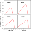 |
Fig. 7 Spatially integrated synchrotron spectra at different ages of the SNR. |
3.3 Non-thermal emission spectra
We considered three non-thermal emission processes: synchrotron emission, IC scattering of CMB photons, and the decay of neutral pions (PD). The methods of calculation are described in Telezhinsky et al. (2013), and Bhatt et al. (2020), respectively. Figures 7 and 9 depict synchrotron spectra and the gamma-ray spectra, respectively, at four points in time. Figure 10 illustrates the energy flux for synchrotron emission and gamma-ray emission during the different evolutionary stages of the remnant. The flux is calculated considering the remnant at a distance of 1 kpc.
The magnetic field strength in our simulation is weak both upstream and downstream of the FS, at least until it reaches the ISM. Therefore, a synchrotron cut-off energy above 100 eV has been achieved only very late in the evolution, but for the first few thousand years, the cut-off energy only reaches near to 50 eV. Turbulent magnetic amplification by streaming instabilities or dynamo action have not been considered, although some evidence for that has been observationally obtained (Ellison 1999; Fang et al. 2013; Zirakashvili et al. 2014).
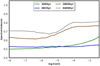 |
Fig. 8 Variation of the spectral index (α) for synchrotron emission with energy at different ages where energy flux (Sv) ∝ v−α. |
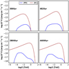 |
Fig. 9 Spatially integrated gamma-ray spectra of PD emission and IC scattering at different ages. |
FS in the free wind
In this region, the flux of both the synchrotron and the hadronic emission decrease with time on account of the declining density, ρ ∝ 1/r2, and also the weakening magnetic field, B ∝ 1/r2. Region 1 in panel a of Fig. 10 demonstrates that the simulated radio flux at 5 GHz energy and the X-ray flux in the range 0.1–10 keV show a power-law decrease with different slopes. It is evident that X-ray emission dominates at the very initial stage of the remnant, but as a consequence of the declining maximum achievable energy of electrons, the X-ray emission fades more quickly than the radio emission, and radio emission starts to dominate after around 1100 yr. In the gamma-ray flux shown in panel b of Fig. 10, interestingly IC emission dominates HE gamma-ray flux except for around initial 60 yr, whereas PD emission dominates in the very high energy (VHE) gamma-ray band. This result reflects the fact that initially the remnant expands through dense material and therefore enhanced PD emission is achieved, and the decreasing electron cut-off energy reduces the VHE IC flux. At the age of 30 00 yr, the synchrotron flux is very low because of the weak magnetic field. Further, the FS propagates through a region of declining density, and consequently the PD emission is also very weak.
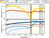 |
Fig. 10 Evolution of energy flux (ø) during the lifetime of SNR for synchrotron emission and gamma-ray emission at specific energy ranges. Region 1, region 2, and region 3 denote the free wind, shocked wind, and shocked ISM region, respectively, which are distinguished by different colours. The brown shaded region around 3200 yr denotes the FS transition from the free wind to the shocked wind zone, and the blue shaded region around 20 000 yr denotes the interaction between FS and LBV shell. |
FS in the shocked wind
As soon as the FS enters this region, the X-ray synchrotron flux starts to grow and eventually dominates over the radio flux on account of the increasing field strength, which is shown in region 2 of panel a of Fig. 10. In this region, both the HE gamma-ray and VHE gamma-ray emissions are dominated by IC scattering, as the remnant expands inside a region of very low density. The non-thermal emission flux fluctuates as the FS interacts with several discontinuities present in this region. For example, the slight increase in HE hadronic emission and radio emission near 20 000 yr depicted in Fig. 10 by the blue shaded region between 17 800 yr and 23 500 yr indicates an interaction between the FS and the LBV shell. The electron spectra are slightly softened, as are the synchrotron spectra. Figure 8 displays the spectral index of synchrotron emission as a function of photon energy. In the radio band, the index is initially around α ≈ 0.53. Figure 9 indicates that after 4820 yr, the roughly constant gas density in the shocked wind moderately boosts the PD emission in comparison to that at the later stage of propagation through the free wind region. IC emission is in spectral agreement with, but at a lower flux than the observed signal from RX J1713.7-3946 (Aharonian et al. 2007; Federici et al. 2015) and Vela Jr. (Sushch et al. 2022). After 28 000 yr, the two- component structure of the synchrotron spectrum, which reflects the break in the electron spectrum, becomes visible and the radio spectral index approaches α ≈ 0.7. The IC emission now extends to the TeV scale and the PD spectrum is rather soft above a few GeV, but shows a weak bump around 1 TeV as a consequence of amplified injection in the LBV shell (cf. Sect. 3.2).
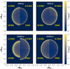 |
Fig. 11 Normalised intensity maps for synchrotron emission: each panel is divided into four segments–the left hemisphere is for radio emission at 1.4-GHz in the upper half and at 14-GHz in the lower half. The right hemisphere is for the 0.3-keV and 3-keV X-ray intensity in the upper half and lower half, respectively. For each segment, the intensity, F/Fm, is normalised to its peak value, Fm. |
FS in the shocked ISM
After entering into the shocked ISM, the FS propagates in a region with a strong magnetic field, which changes the synchrotron spectra. Our calculated X-ray flux dominates over radio flux in this region also, and although the hadronic HE emission starts to grow in this region, both the HE and VHE gamma-ray emission have a leptonic origin, illustrated in Fig. 10 inside region 3. We observe very soft spectra from the radio band (α ≈ 0.71) to the infrared (α ≈ 0.83). Additionally, the spectral index for PD emission above 10 GeV reflects the softness of the proton spectra (spectral index ≈2.6). Correspondingly, soft gamma-ray has been observed from IC 443 and W44, both of which expand in a dense molecular cloud (Fang et al. 2013; Cardillo et al. 2014). The obtained soft radio spectra in our simulation are relatively consistent with the data for many Galactic SNRs (Baars et al. 1977; Green 2009; Urošević 2014; Domček et al. 2021).
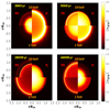 |
Fig. 12 Normalised intensity maps of PD and IC The segments are organised to distinguish the photon energy: 10 GeV in the upper half and 1 TeV in the lower half, and PD on the left hemisphere and IC on the right hemisphere. In each segment, the intensity, F/Fm, is normalised to its peak value, Fm. |
3.4 Morphology of non-thermal emission
We calculated intensity maps for synchrotron emission and gamma-ray emission (see Fig. 11 and Fig. 12, respectively), respectively, for a fiducial distance of 1000 parsecs. To be noted from the figures is the evident variation of the source morphology with the age of the SNR. The X-ray morphology (0.3 KeV and 3 KeV) features a thin shell throughout the entire lifetime of the SNR whereas the radio morphology (1.4-GHz and 14-GHz) shows a comparatively thicker shell and eventually becomes moderately centre-filled when the FS is in the shocked wind, shown at 28 000 yr in Fig. 11. After 3000 yr, when the FS propagates through the free stellar wind, the brightest synchrotron emission in both the radio and the X-ray band emanate from the contact discontinuity between the FS and the RS on account of the strong magnetic field there (cf. Lyutikov & Pohl 2004). At a later stage, when the FS passes through the shocked stellar wind, the synchrotron morphology is essentially the same as at earlier times. After 28 000 yr, when the FS is still inside the shocked wind but approaches the CD between the wind bubble and the ISM and already interacted with the LBV shell, the brightest radio emission comes from the region near the contact discontinuity between the FS and the RS as well as the region near the LBV shell whereas the CD of the wind bubble appears X-ray bright as there the magnetic field is 12 times stronger than that immediately downstream of the FS. After 44000 yr, when the FS is located in the shocked ISM, the highest radio intensity emanates from a region near the LBV shell whereas the X-ray emission comes from immediately downstream of the FS. The magnetic field downstream of the FS is with a strength below 1 µ G, too weak to produce significant radio emission, but the remnant appears as somewhat centre-filled in the radio band as a consequence of diffusion of the electrons in the deep downstream. In the gamma-ray band, the IC morphology shows a thick shell whereas the PD emission appears centre-filled at earlier evolutionary stages of the remnant inside the free wind, which is illustrated in Fig. 12 at 3000 yr. The maximum IC intensity emanates from the region around the FS for both energies and the interior of the remnant also appears brighter as weak magnetic field downstream of the FS allows electrons to deeply penetrate. PD emission primarily comes from two regions: the dense ejecta in the interior of the SNR and a broad region near the contact discontinuity between the FS and the RS. Later, at 9500 yr, the IC intensity at 10 GeV comes from the entire region downstream of the FS, and at 1 TeV the IC intensity is the highest in a shell located immediately downstream of the FS. Similarly, the PD emission is seen from almost the entire region interior of the FS, and at TeV energies most of the flux comes from the SNR ejecta. At 28 000 yr, the entire region inside the RS is IC bright, specifically where the magnetic field is weak, whereas the PD emission at both 10 GeV and 1 TeV feature shell-like structure. The TeV shell is located at the wind bubble CD, while at 10 GeV the highest PD intensity comes from the region around the LBV shell. Finally, after FS and wind bubble CD interaction, the IC emission appears centre-filled inside the RS, as it did at early times, and PD emission shows a shell-like morphology, as depicted in Fig. 12 at 44 000 yr.
In reality, the emission maps will be more complex and patchy, because the distinct shell-like morphology reflects the spherical symmetry in our 1D simulations. In particular, the Rayleigh-Taylor instability (Fraschetti et al. 2010) may break the contact discontinuities in the wind bubble and in the SNR into fragments.
4 Conclusions
We explored the structure of the wind bubble created by a 60 M⊙ star with solar metallicity formed by the mass-loss of the star from the ZAMS phase to the pre-supernova stage to study the interactions of the eventual SNR shock with the modified CSM during its passage through the wind bubble. Our simulations of particle acceleration at the FS of the SNR suggest that the spectra and flux of energetic particles in core-collapse SNRs are significantly influenced by the structure of the wind bubble. The modification in particle acceleration is thus intertwined with the evolution history of the progenitor star and depends on its properties, such as the ZAMS mass, the metallicity, and the rotation. Our simulations demonstrate the impact of the various discontinuities, including the wind-termination shock, a dense LBV shell, and the wind bubble CD, and also the effect of shock-merging on particle acceleration.
The spectra of accelerated particles depend on the interactions of the FS with the CSM as well as the CSM magnetic-field model. Throughout the propagation of the FS in the hot wind bubble and shocked ISM, beginning at an age of about 3300 yr, softer particle spectra are persistently observed because of the relatively small sonic Mach number of the forward shock. For protons above 10 GeV energy, the spectral index reaches around 2.5. Further, the total production spectrum released into the ISM, calculated at 46 000 yr, follows a broken power-law with a spectral index of s ≈ 2.4–2.5 above 10 GeV energy. This is broadly consistent with the spectral shape of the injection spectrum at higher energy required by propagation models for the Galactic CRs (Strong et al. 2000, 2007). In addition to the effect of discussed small Mach number of the FS, neutral particles (Ohira et al. 2009; Ohira & Takahara 2010) in the shocked ISM as well as the non-linear study of DSA (Drury & Voelk 1981; Berezhko & Ellison 1999; Malkov & Drury 2001) may also have significant impacts on particle acceleration but considering both of these aspects is beyond the scope of this paper.
The spectra and morphology of non-thermal emission reflects the spectral distribution of particles. The gamma-ray emission in our model is dominated by the leptonic contributions, and even that provides a relatively low flux. The PD emission is likely not observable, but has a two-component structure in the spectrum after the interaction of FS with the LBV shell. This feature should be brighter and therefore possibly observable if the progenitor star was in a high-density environment. The IC morphology varies between shell-enhanced and centre- filled, whereas the PD emission has a centre-filled to shell-like morphology. It is challenging to detect an extended object with radius exceeding 80 pc after 45 000 yr (5° for a distance of 1 kpc) with a flux as low as we calculate. The flux may be higher for a high-density ISM and for efficient magnetic-field amplification in the remnant, and so there is a possibility that we may be able to observe this with the next generation of observatories, such as SKA, CTA, and LHAASO. Although our simulation of an SNR of a progenitor with 60 M⊙ ZAMS mass is entirely based on theoretical reasoning, our analysis offers information that can be used to further understand SNR G150.3+4.5 (discussed in Devin et al. 2020) with angular size ~3°. The very high shock velocity expected for this extended SNR expanding in a low ambient density suggests a core-collapse scenario with a large wind bubble and that the FS is expanding in the shocked wind. The predicted maximum cut-off energy for particles (5 TeV) and softer radio spectral index from some regions of this extended SNR are consistent with the results of our simulation. Additionally, we also find an IC-dominated γ-ray spectrum as predicted for SNR G150.3+4.5. In conclusion, we investigated the evolution of an SNR with a WR progenitor considering Bohm-scaling of diffusion downstream and immediately upstream of the FS. Berezhko & Völk (2000) estimated the maximum energy for accelerated protons and the cut-off energy for expected gamma-ray flux to be 1014 eV and 1013 eV, respectively, considering Bohm diffusion during the expansion of an SNR with a WR progenitor and an ejecta mass comparable to that in our simulation. Although our model yields consistent results, the Bohm limit for CR diffusion may be too optimistic. Considering CR streaming instability and Kolmogorov non-linearity in magneto-hydrodynamic waves, (Ptuskin & Zirakashvili 2003, 2005) estimated analytically that for the ejecta-dominated stage the maximum energy may exceed the ‘knee’ but at the later Sedov phase it can be reduced to 10 GeV. A future study including a diffusion model based on the resonant streaming instability and magnetic field amplification may indicate additional observational signatures.
Acknowledgements
The authors acknowledge the North-German Supercomputing Alliance (HLRN) for providing HPC resources to perform the hydrodynamic simulation from ZAMS to pre-supernova stage of the star. Iurii Sushch acknowledges support by the National Research Foundation of South Africa (grant No. 132276). Robert Brose acknowledges funding from an Irish Research Council Starting Laureate Award (IRCLA/2017/83).
Appendix A Effect of shock-shock tail-on interactions on particle spectra
When a reflected shock catches up with the FS, there is a limited time window of duration ti in which particles might be able to diffusively cross both shocks and thus probe the full compression ratio of the two-shock system. That compression ratio across both shocks is typically larger than four, and therefore a spectral hardening could be expected. However, to have any effect on the spectrum, the interaction time, ti, needs to be longer than the acceleration time of particles. Particles crossing the trailing shock toward the upstream region can reach the leading shock, if it is located within the characteristic distance L that is given by,
 (A.1)
(A.1)
where D1,2 is the spatial diffusion coefficient of particles between two shocks at a given energy and Vsh,2 is the speed of the trailing shock. Therefore, the time to collision is
 (A.2)
(A.2)
where Δυ denotes the difference in the propagation speed between both shocks. It can be related to the speed of the two shocks,
 (A.3)
(A.3)
where κ1 is the compression ratio of the leading shock. Assuming the first shock is strong, κ1 = 4, and an adiabatic index γ = 5/3, the sonic Mach number of the second shock is
 (A.4)
(A.4)
Having a trailing shock (M2 > 1) requires that  1)/4, and so the time to collision cannot be made arbitrarily long. We can now express the interaction time in terms of Vsh,1 and M2,
 (A.5)
(A.5)
The total compression at the two-shock system is (again for κ1 = 4)
 (A.6)
(A.6)
where a negative value implies that the far-downstream flow is faster than the first shock. It is evident that a very moderate Mach number of the trailing shock, M2, is sufficient to significantly raise the total compression ratio, Ktot » 4, which would with time lead to very hard particle spectra. The question is whether or not there is sufficient time to establish such a hard spectrum.
We can extend the analysis of Drury (1991) to see that the relative momentum gain per shock-acceleration cycle,
 (A.7)
(A.7)
is only weakly enhanced at the two-shock system, whatever the total compression. The mean residence time downstream of the leading shock is
 (A.8)
(A.8)
Article number, page 12 of 13
where in the absence of the trailing shock Vd = Vsh,1/κ1. Downstream of the trailing shock, the flow speed and possibly the diffusion coefficient will change. For constant flow speed and diffusion coefficient between the shocks, and integrating only over the distance between the shocks, L, we obtain a strict lower limit to the duration of an acceleration cycle,
![Mathematical equation: ${t_c} > {{16{D_{1,2}}} \over {c{V_{{\rm{sh,1}}}}}}\left[{1 - {\rm{exp}}\left({- {1 \over {\sqrt 5 {M_2}}}} \right)} \right],$](/articles/aa/full_html/2022/05/aa42747-21/aa42747-21-eq29.png) (A.9)
(A.9)
where we used equations A.1 and A.4. The acceleration-time, ta = tc p/Δp, of a particle is
![Mathematical equation: $\matrix{{{t_a}} \hfill & \mathbin{\lower.3ex\hbox{$\buildrel>\over {\smash{\scriptstyle\sim}\vphantom{_x}}$}} \hfill & {12{{{D_{1,2}}} \over {V_{{\rm{sh,1}}}^2}}{{{\kappa_{{\rm{tot}}}}} \over {{\kappa_{{\rm{tot}}}} - 1}}\left[{1 - {\rm{exp}}\left({- {1 \over {\sqrt 5 {M_2}}}} \right)} \right]} \hfill \cr {} \hfill & \simeq \hfill & {{{12} \over {\sqrt 5 {M_2}}}{{{D_{1,2}}} \over {V_{{\rm{sh,1}}}^2}}{{{\kappa_{{\rm{tot}}}}} \over {{\kappa_{{\rm{tot}}}} - 1}}.} \hfill \cr}$](/articles/aa/full_html/2022/05/aa42747-21/aa42747-21-eq30.png) (A.10)
(A.10)
Comparison with eq. A.6 yields the ratio of the relevant timescales, which is given by
 (A.11)
Given that we ignored time spent upstream of the leading shock or downstream of the trailing shock, we can conclude that particles can see the full compression of both shocks combined for less than a single acceleration time. A similar result is found for the post-collision phase, when the two shocks move in opposite direction and separate very quickly, as well as for head-on collisions. All in all, tail-on shock collisions cannot produce significant spectral features.
Appendix B Animation of the evolution of FS inside the wind bubble
Figure B.1 includes flow number density(n) and magnetic field configuration (B) in the vicinity of FS along with the shock compression ratio (Cr), shock velocity (Vsh), and proton, electron, and non-thermal emission spectra for the entire time-span of the simulation at different time-steps.
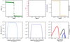 |
Fig. B.1 Evolution of FS. (i) Upper row: The left panel illustrates the gas density, n, as a function of radius, the second panel shows the compression ratio, Cr, and the speed of the shock, Vsh, as functions of time, and the third panel depicts the magnetic-field strength near the shock, B. Theblack vertical line denotes the position of the SNR FS. (ii) Lower row: The first panel shows proton (Pr) spectra volume-averaged downstream of the FS. The corresponding electron (El) spectra are illustrated in the second panel. The third panel shows the spectra of synchrotron emission (red), IC emission (black) and PD emission (blue). |
References
- Abdo, A. A., Ackermann, M., Ajello, M., et al. 2010, ApJ, 710, L92 [NASA ADS] [CrossRef] [Google Scholar]
- Acciari, V. A., Aliu, E., Arlen, T., et al. 2009, ApJ, 698, L133 [NASA ADS] [CrossRef] [Google Scholar]
- Acciari, V. A., Aliu, E., Arlen, T., et al. 2011, ApJ, 730, L20 [NASA ADS] [CrossRef] [Google Scholar]
- Acero, F., Aharonian, F., Akhperjanian, A. G., et al. 2010, A&A, 516, A62 [NASA ADS] [CrossRef] [EDP Sciences] [Google Scholar]
- Aharonian, F., Akhperjanian, A. G., Bazer-Bachi, A. R., et al. 2007, A&A, 464, 235 [NASA ADS] [CrossRef] [EDP Sciences] [Google Scholar]
- Baade, W., & Zwicky, F. 1934, Proc. Natl. Acad. Sci. U.S.A., 20, 259 [NASA ADS] [CrossRef] [Google Scholar]
- Baars, J. W. M., Genzel, R., Pauliny-Toth, I. I. K., & Witzel, A. 1977, A&A, 61, 99 [NASA ADS] [Google Scholar]
- Bell, A. R. 1978, MNRAS, 182, 147 [Google Scholar]
- Berezhko, E. G., & Ellison, D. C. 1999, ApJ, 526, 385 [Google Scholar]
- Berezhko, E. G., & Völk, H. J. 2000, A&A, 357, 283 [NASA ADS] [Google Scholar]
- Berezinskii, V. S., & Ptuskin, V. S. 1989, A&A, 215, 399 [NASA ADS] [Google Scholar]
- Bhatt, M., Sushch, I., Pohl, M., et al. 2020, Astropart. Phys., 123, 102490 [NASA ADS] [CrossRef] [Google Scholar]
- Blasi, P. 2013, A&ARr, 21, 70 [NASA ADS] [CrossRef] [Google Scholar]
- Blasi, P., Gabici, S., & Vannoni, G. 2005, MNRAS, 361, 907 [NASA ADS] [CrossRef] [Google Scholar]
- Borkowski, K., Szymkowiak, A. E., Blondin, J. M., & Sarazin, C. L. 1996, ApJ, 466, 866 [NASA ADS] [CrossRef] [Google Scholar]
- Brecher, K., & Burbidge, G. R. 1972, ApJ, 174, 253 [NASA ADS] [CrossRef] [Google Scholar]
- Brose, R., Telezhinsky, I., & Pohl, M. 2016, A&A, 593, A20 [NASA ADS] [CrossRef] [EDP Sciences] [Google Scholar]
- Brose, R., Pohl, M., Sushch, I., Petruk, O., & Kuzyo, T. 2020, A&A, 634, A59 [EDP Sciences] [Google Scholar]
- Brose, R., Pohl, M., & Sushch, I. 2021, A&A, 654, A139 [NASA ADS] [CrossRef] [EDP Sciences] [Google Scholar]
- Büsching, I., Pohl, M., & Schlickeiser, R. 2001, A&A, 377, 1056 [NASA ADS] [CrossRef] [EDP Sciences] [Google Scholar]
- Cardillo, M., Tavani, M., Giuliani, A., et al. 2014, A&A, 565, A74 [NASA ADS] [CrossRef] [EDP Sciences] [Google Scholar]
- Cardillo, M., Amato, E., & Blasi, P. 2016, A&A, 595, A58 [NASA ADS] [CrossRef] [EDP Sciences] [Google Scholar]
- Caprioli, D., Haggerty, C. C., & Blasi, P. 2020, ApJ, 905, 2 [Google Scholar]
- Cassinelli, J. P. 1991, in Wolf-Rayet Stars and Interrelations with Other Massive Stars in Galaxies, eds. K. A. van der Hucht, & B. Hidayat, 143, 289 [NASA ADS] [CrossRef] [Google Scholar]
- Celli, S., Morlino, G., Gabici, S., & Aharonian, F. A. 2019, MNRAS, 490, 4317 [CrossRef] [Google Scholar]
- Chené, A. N. & St-Louis, N. 2010, ApJ, 716, 929 [CrossRef] [Google Scholar]
- Chevalier, R. A., & Liang, E. P. 1989, ApJ, 344, 332 [NASA ADS] [CrossRef] [Google Scholar]
- Chevalier, R. A., & Luo, D. 1994, ApJ, 421, 225 [NASA ADS] [CrossRef] [Google Scholar]
- Chiotellis, A., Boumis, P., & Spetsieri, Z. T. 2021, MNRAS, 502, 176 [NASA ADS] [CrossRef] [Google Scholar]
- Ciotti, L., & D’Ercole, A. 1989, A&A, 215, 347 [NASA ADS] [Google Scholar]
- Crowther, P. A. 2007, ARA&A, 45, 177 [Google Scholar]
- de Oña Wilhelmi, E., Sushch, I., Brose, R., et al. 2020, MNRAS, 497, 3581 [CrossRef] [Google Scholar]
- Devin, J., Lemoine-Goumard, M., Grondin, M. H., et al. 2020, A&A, 643, A28 [NASA ADS] [CrossRef] [EDP Sciences] [Google Scholar]
- Domček, V., Vink, J., Hernández Santisteban, J. V., DeLaney, T., & Zhou, P. 2021, MNRAS, 502, 1026 [CrossRef] [Google Scholar]
- Drury, L. O. 1983, Rep. Prog. Phys., 46, 973 [Google Scholar]
- Drury, L. O. 1991, MNRAS, 251, 340 [NASA ADS] [CrossRef] [Google Scholar]
- Drury, L. O., & Voelk, J. H. 1981, ApJ, 248, 344 [NASA ADS] [CrossRef] [Google Scholar]
- Dwarkadas, V. V. 2005, ApJ, 630, 892 [NASA ADS] [CrossRef] [Google Scholar]
- Dwarkadas, V. V. 2007, ApJ, 667, 226 [NASA ADS] [CrossRef] [Google Scholar]
- Ellison, D. 1999, in International Cosmic Ray Conference, 3, 26th International Cosmic Ray Conference (ICRC26), eds. D.B. Kieda, M.B. Salamon, B.L. Dingus, 468 [NASA ADS] [Google Scholar]
- Ellison, D. C., Drury, L. O., & Meyer, J.-P. 1997, ApJ, 487, 197 [NASA ADS] [CrossRef] [Google Scholar]
- Ellison, D. C., Decourchelle, A., & Ballet, J. 2005, A&A, 429, 569 [NASA ADS] [CrossRef] [EDP Sciences] [Google Scholar]
- Fang, J., Yu, H., Zhu, B.-T., & Zhang, L. 2013, MNRAS, 435, 570 [NASA ADS] [CrossRef] [Google Scholar]
- Federici, S., Pohl, M., Telezhinsky, I., Wilhelm, A., & Dwarkadas, V. V. 2015, A&A, 577, A12 [NASA ADS] [CrossRef] [EDP Sciences] [Google Scholar]
- Fermi, E. 1949, Phys. Rev., 75, 1169 [NASA ADS] [CrossRef] [Google Scholar]
- Fraschetti, F., Teyssier, R., Ballet, J., & Decourchelle, A. 2010, A&A, 515, A104 [NASA ADS] [CrossRef] [EDP Sciences] [Google Scholar]
- García-Segura, G., Langer, N., Rózyczka, M., Franco, J., & Mac Low, M. M. 1999, in Wolf-Rayet Phenomena in Massive Stars and Starburst Galaxies, eds. K.A. van der Hucht, G. Koenigsberger, & P.R.J. Eenens, 193, 325 [Google Scholar]
- Green, D. A. 2009, Bull. Astron. Soc. India, 37, 45 [NASA ADS] [Google Scholar]
- Groh, J. H., Meynet, G., Ekström, S., & Georgy, C. 2014, A&A, 564, A30 [NASA ADS] [CrossRef] [EDP Sciences] [Google Scholar]
- Guyer, J. E., Wheeler, D., & Warren, J. A. 2009, Comput. Sci. Eng., 11, 6 [NASA ADS] [CrossRef] [Google Scholar]
- Ignace, R., Cassinelli, J. P., & Bjorkman, J. E. 1996, ApJ, 459, 671 [NASA ADS] [CrossRef] [Google Scholar]
- Ignace, R., Cassinelli, J. P., & Bjorkman, J. E. 1998, ApJ, 505, 910 [NASA ADS] [CrossRef] [Google Scholar]
- Inoue, T., Marcowith, A., Giacinti, G., Jan van Marle, A., & Nishino, S. 2021, ApJ, 922, 7 [NASA ADS] [CrossRef] [Google Scholar]
- Jennings, Z. G., Williams, B. F., Murphy, J. W., et al. 2014, ApJ, 795, 170 [NASA ADS] [CrossRef] [Google Scholar]
- Kang, H., & Ryu, D. 2010, ApJ, 721, 886 [NASA ADS] [CrossRef] [Google Scholar]
- Lagage, P. O., & Cesarsky, C. J. 1983, A&A, 125, 249 [NASA ADS] [Google Scholar]
- Lyutikov, M., & Pohl, M. 2004, ApJ, 609, 785 [NASA ADS] [CrossRef] [Google Scholar]
- Mackey, J., Green, S., & Moutzouri, M. 2020, in Journal of Physics Conference Series, 1620, 012012 [NASA ADS] [CrossRef] [Google Scholar]
- Malkov, M. A., & Drury, L. O. 2001, Rep. Progr. Phys., 64, 429 [Google Scholar]
- Malkov, M. A., Diamond, P. H., & Sagdeev, R. Z. 2011, Nat. Commun., 2, 194 [NASA ADS] [CrossRef] [Google Scholar]
- Meyer, D. M. A., Petrov, M., & Pohl, M. 2020, MNRAS, 493, 3548 [CrossRef] [Google Scholar]
- Meyer, D. M. A., Pohl, M., Petrov, M., & Oskinova, L. 2021, MNRAS, 502, 5340 [NASA ADS] [CrossRef] [Google Scholar]
- Mignone, A., Bodo, G., Massaglia, S., et al. 2007, ApJS, 170, 228 [Google Scholar]
- Ohira, Y., & Takahara, F. 2010, ApJ, 721, L43 [NASA ADS] [CrossRef] [Google Scholar]
- Ohira, Y., Terasawa, T., & Takahara, F. 2009, ApJ, 703, L59 [NASA ADS] [CrossRef] [Google Scholar]
- Pohl, M., Wilhelm, A., & Telezhinsky, I. 2015, A&A, 574, A43 [NASA ADS] [CrossRef] [EDP Sciences] [Google Scholar]
- Ptuskin, V. S., & Zirakashvili, V. N. 2003, A&A, 403, 1 [NASA ADS] [CrossRef] [EDP Sciences] [Google Scholar]
- Ptuskin, V. S., & Zirakashvili, V. N. 2005, A&A, 429, 755 [NASA ADS] [CrossRef] [EDP Sciences] [Google Scholar]
- Schure, K. M., Achterberg, A., Keppens, R., & Vink, J. 2010, MNRAS, 406, 2633 [NASA ADS] [CrossRef] [Google Scholar]
- Simpson, C. M., Pakmor, R., Marinacci, F., et al. 2016, ApJ, 827, L29 [NASA ADS] [CrossRef] [Google Scholar]
- Strong, A. W., Moskalenko, I. V., & Reimer, O. 2000, ApJ, 537, 763 [NASA ADS] [CrossRef] [Google Scholar]
- Strong, A. W., Moskalenko, I. V., & Ptuskin, V. S. 2007, Ann. Rev. Nucl. Part. Sci., 57, 285 [NASA ADS] [CrossRef] [Google Scholar]
- Sushch, I., Brose, R., & Pohl, M. 2022, A&A, 618, A155 [Google Scholar]
- Sushch, I., Brose, R., Pohl, M., Plotko, P., & Das, S. 2022, ApJ, 926, 140 [NASA ADS] [CrossRef] [Google Scholar]
- Telezhinsky, I., Dwarkadas, V. V., & Pohl, M. 2012a, Astropart. Phys., 35, 300 [NASA ADS] [CrossRef] [Google Scholar]
- Telezhinsky, I., Dwarkadas, V. V., & Pohl, M. 2012b, A&A, 541, A153 [NASA ADS] [CrossRef] [EDP Sciences] [Google Scholar]
- Telezhinsky, I., Dwarkadas, V. V., & Pohl, M. 2013, A&A, 552, A102 [NASA ADS] [CrossRef] [EDP Sciences] [Google Scholar]
- Urošević, D. 2014, Ap&SS, 354, 541 [Google Scholar]
- Ustamujic, S., Orlando, S., Miceli, M., et al. 2021, A&A, 654, A167 [NASA ADS] [CrossRef] [EDP Sciences] [Google Scholar]
- Vaidya, B., Mignone, A., Bodo, G., Rossi, P., & Massaglia, S. 2018, ApJ, 865, 144 [Google Scholar]
- van Marle, A. J., Meliani, Z., & Marcowith, A. 2015, A&A, 584, A49 [CrossRef] [EDP Sciences] [Google Scholar]
- Vieu, T., Gabici, S., & Tatischeff, V. 2020, MNRAS, 494, 3166 [NASA ADS] [CrossRef] [Google Scholar]
- Voelk, H. J., & Biermann, P. L. 1988, ApJ, 333, L65 [CrossRef] [Google Scholar]
- Wilhelm, A., Telezhinsky, I., Dwarkadas, V. V., & Pohl, M. 2020, A&A, 639, A124 [NASA ADS] [CrossRef] [EDP Sciences] [Google Scholar]
- Zirakashvili, V. N., Aharonian, F. A., Yang, R., Oña-Wilhelmi, E., & Tuffs, R. J. 2014, ApJ, 785, 130 [NASA ADS] [CrossRef] [Google Scholar]

We cut the grid of the pre-supernova CSM because we follow the SNR shock only to the shocked ISM. Additionally, we increased by interpolation the grid resolution from 50 000 cells to 262 144 cells.
All Figures
|
Fig. 1 Profiles of the number density (n, panel a), the flow speed (u, panel b), the thermal pressure (P, panel c), and the temperature (T, panel d) immediately after the supernova explosion. Vertical grey lines mark the boundary of the supernova ejecta (up to 0.023 parsec), the free stellar wind (region 1), the shocked LBV and WR wind (region 2), the shocked wind from the O and B phases (region 3), the shocked ISM (region 4), and the ambient ISM (region 5). RWT is the radius of the wind termination shock, LBV shell denotes the dense shell created by interaction between LBV wind and WR wind, and CD represents the contact discontinuity between shocked wind and shocked ISM. |
| In the text | |
|
Fig. 2 Behaviour of FS parameters: radius (Rsh), velocity (Vsh), and shock compression ratio (CrRATPaC). In the upper panel, we also provide the angular scale, θsh, for a distance of 1000 parsec. (i)-(iv) mark interactions of the FS with different discontinuities, namely (i) the wind termination shock, (ii) another outgoing shock, (iii) the LBV shell, and (iv) the CD. |
| In the text | |
|
Fig. 3 Proton spectra volume-averaged downstream of the FS at early times: for context, we also provide the gas number density, n, as a function of radius. The second row displays the compression ratio (CrRATPaC) and the shock speed (Vsh) up to the specific age, the third row depicts the magnetic-field profile (B), and the fourth row illustrates the proton spectra. The vertical lines in the first and the third row mark the FS position. |
| In the text | |
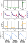 |
Fig. 4 Proton spectra volume-averaged downstream of the FS as in Fig. 3, but for later times. |
| In the text | |
|
Fig. 5 Variation of the spectral index for protons at different ages with momentum of SNR. |
| In the text | |
|
Fig. 6 Electron spectra at different ages of the SNR, volume-averaged downstream of the FS. |
| In the text | |
|
Fig. 7 Spatially integrated synchrotron spectra at different ages of the SNR. |
| In the text | |
|
Fig. 8 Variation of the spectral index (α) for synchrotron emission with energy at different ages where energy flux (Sv) ∝ v−α. |
| In the text | |
|
Fig. 9 Spatially integrated gamma-ray spectra of PD emission and IC scattering at different ages. |
| In the text | |
|
Fig. 10 Evolution of energy flux (ø) during the lifetime of SNR for synchrotron emission and gamma-ray emission at specific energy ranges. Region 1, region 2, and region 3 denote the free wind, shocked wind, and shocked ISM region, respectively, which are distinguished by different colours. The brown shaded region around 3200 yr denotes the FS transition from the free wind to the shocked wind zone, and the blue shaded region around 20 000 yr denotes the interaction between FS and LBV shell. |
| In the text | |
|
Fig. 11 Normalised intensity maps for synchrotron emission: each panel is divided into four segments–the left hemisphere is for radio emission at 1.4-GHz in the upper half and at 14-GHz in the lower half. The right hemisphere is for the 0.3-keV and 3-keV X-ray intensity in the upper half and lower half, respectively. For each segment, the intensity, F/Fm, is normalised to its peak value, Fm. |
| In the text | |
|
Fig. 12 Normalised intensity maps of PD and IC The segments are organised to distinguish the photon energy: 10 GeV in the upper half and 1 TeV in the lower half, and PD on the left hemisphere and IC on the right hemisphere. In each segment, the intensity, F/Fm, is normalised to its peak value, Fm. |
| In the text | |
|
Fig. B.1 Evolution of FS. (i) Upper row: The left panel illustrates the gas density, n, as a function of radius, the second panel shows the compression ratio, Cr, and the speed of the shock, Vsh, as functions of time, and the third panel depicts the magnetic-field strength near the shock, B. Theblack vertical line denotes the position of the SNR FS. (ii) Lower row: The first panel shows proton (Pr) spectra volume-averaged downstream of the FS. The corresponding electron (El) spectra are illustrated in the second panel. The third panel shows the spectra of synchrotron emission (red), IC emission (black) and PD emission (blue). |
| In the text | |
Current usage metrics show cumulative count of Article Views (full-text article views including HTML views, PDF and ePub downloads, according to the available data) and Abstracts Views on Vision4Press platform.
Data correspond to usage on the plateform after 2015. The current usage metrics is available 48-96 hours after online publication and is updated daily on week days.
Initial download of the metrics may take a while.