| Issue |
A&A
Volume 660, April 2022
|
|
|---|---|---|
| Article Number | L2 | |
| Number of page(s) | 6 | |
| Section | Letters to the Editor | |
| DOI | https://doi.org/10.1051/0004-6361/202243299 | |
| Published online | 30 March 2022 | |
Letter to the Editor
Gravity darkening and tidally perturbed stellar pulsation in the misaligned exoplanet system WASP-33
1
Konkoly Observatory, Research Centre for Astronomy and Earth Sciences, Eötvös Loránd Research Network (ELKH), Konkoly-Thege Miklós út 15-17, 1121 Budapest, Hungary
2
MTA-ELTE Exoplanet Research Group, Szent Imre h. u. 112, 9700 Szombathely, Hungary
3
ELTE Eötvös Loránd University, Doctoral School of Physics, Pázmány Péter sétány 1/A, 1117 Budapest, Hungary
e-mail: This email address is being protected from spambots. You need JavaScript enabled to view it.
4
University of Szeged, Department of Optics and Quantum Electronics, Institute of Physics, Dóm tér 9, 6720 Szeged, Hungary
5
ELTE Eötvös Loránd University, Gothard Astrophysical Observatory, Szent Imre h. u. 112, 9700 Szombathely, Hungary
6
MTA-ELTE Lendület “Momentum” Milky Way Research Group, Hungary
7
University of Szeged, Institute of Physics, Dóm tér 9, 6720 Szeged, Hungary
8
University of Szeged, Doctoral School of Physics, Dóm tér 9, 6720 Szeged, Hungary
Received:
9
February
2022
Accepted:
12
March
2022
Abstract
Aims. WASP-33 is one of the few δ Sct stars with a known planetary companion. By analyzing the stellar oscillations, we search for possible star-planet interactions in the pattern of the pulsation.
Methods. We made use of the Transit and Light Curve Modeller to solve the light curve from the Transiting Exoplanet Survey Satellite. We include gravity darkening in our analysis.
Results. The stellar oscillation pattern of WASP-33 clearly shows signs of several tidally perturbed modes. We find that there are peaks in the frequency spectrum that are at or near the 3rd, 12th, and 25th orbital harmonics (forb ∼ 0.82 d−1). Also, there is a prominent overabundance of pulsational frequencies rightward of the orbital harmonics, a characteristic of a tidally perturbed stellar pulsation, which is an outcome of star-planet interactions in the misaligned system. There are peaks in both the δ Sct and γ Dor ranges of the Fourier spectrum, implying that WASP-33 is a γ Dor – δ Sct hybrid pulsator. The transit light curves are best fitted by a gravity-darkened stellar model, and the planet parameters are consistent with earlier determinations.
Key words: techniques: photometric / planets and satellites: general / stars: variables: δ Scuti
© ESO 2022
1. Introduction
The known δ Sct sample from the Kepler (Borucki et al. 2010) field has been explored by Hey et al. (2021), who found only 20 planet candidates in total, shedding light on a notable lack of planetary companions to such stars. This remains true even in the era of space-based transiting exoplanet photometry with satellites such as the Transiting Exoplanet Survey Satellite (TESS; Ricker et al. 2015) and the CHaraterizing ExOplanet Satellite (CHEOPS, Benz et al. 2021): there is a notable lack of planets orbiting δ Scuti stars. Hey et al. (2021) explored the known δ Sct sample from the Kepler (Borucki et al. 2010) field and found 20 planet candidates in total.
The planetary companion of WASP-33 is a hot Jupiter with P ∼ 1.219867 ± 4.2 ⋅ 10−5 days (von Essen et al. 2020), MP ∼ 2.10 ± 0.14MJ, and RP ∼ 1.59 ± 0.07RJ (Chakrabarty & Sengupta 2019). WASP-33b (Christian et al. 2006) was the first confirmed planet orbiting a δ Sct host star (Herrero et al. 2011), and it has been analyzed thoroughly, including via Doppler tomography and radial velocity measurements (Collier Cameron et al. 2010; Watanabe et al. 2020; Borsa et al. 2021) as well as ground-based photometry (von Essen et al. 2014). Using the TESS light curve, von Essen et al. (2020) improved the precision of the known transit parameters. Dholakia et al. (2022) argued that after subtracting the pulsation from the TESS light curve, an asymmetry emerges during the transits that is characteristic of a gravity-darkened stellar disk.
In this paper we reexamine the TESS light curve of WASP-33, including gravity darkening in our analysis. We also investigate the possibility of star-planet interactions. This paper is structured as follows. In Sect. 2 we describe our model for the transit in both the gravity-darkened and non-gravity-darkened cases. In Sect. 3 we reanalyze the TESS light curve of the WASP-33 system using the Transit and Light Curve Modeller (TLCM; Csizmadia 2020) without pre-whitening the data. We make use of the wavelet formulation built into TLCM to handle the pulsations and the transit light curve simultaneously. We also reconstruct the Fourier spectra of the stellar oscillations from the fitted light curve, which allows us to investigate the possibility of planet-star interactions.
2. Light curve analysis
2.1. Light curve preparation
The WASP-33 system has been observed in TESS1 Sector 18. Using the lightkurve python package (Lightkurve Collaboration 2018), we downloaded the PDCSAP (Pre-search Data Conditioning Simple Aperture Photometry) data produced by the automated pipeline of the mission. We removed the first 781 points due to an artifact that could bias the analysis of the first transit event and detrended the light curve. We were eventually left with a data set of 14 028 measurements consisting of TESS short cadence observations, which included 16 transits of WASP-33b.
2.2. Light curve solutions
Stellar oscillations and any possible instrumental effects severely distort the transit light curve of WASP-33b. In order to compensate for these effects, we employed the wavelet-based routines of Carter & Winn (2009), which are built into TLCM. These describe the time-correlated noise (i.e., pulsation and systematics) in terms of two parameters: σr for the red component and σw for the white component (see Carter & Winn 2009 for details). Csizmadia et al. (2021) proved the validity of this approach, while Kálmán et al. (2021) completed an extensive test for the consistency of transit parameter estimation using TLCM. This code allows the simultaneous fitting of the noise and the transit. The transit modeling is carried out via the analytic model of Mandel & Agol (2002), which is described by the ratio of the planetary and stellar radii, RP/RS, the scaled semimajor axis, a/RS, the impact parameter, b = a/RScosi (where i is the orbital inclination relative to the line of sight), and the time of mid-transit, tC.
Gravity darkening of the host star causes asymmetric transit light curves (Barnes 2009). This phenomenon, as implemented by TLCM, is described by three parameters (Csizmadia et al. 2021): the gravity darkening exponent, β, the inclination of the stellar rotational axis (measured from the line of sight), i⋆, and the projected spin orbit angle, λ. In order to perform a thorough analysis of the WASP-33b light curve, we considered three different scenarios: (i) no gravity darkening (despite the rapid rotation of WASP-33 at vsini⋆ = 86.5 km s−1; Johnson et al. 2015), (ii) with the gravity darkening exponent fixed to its nominal value, 0.25 (von Zeipel 1924), and i⋆ and λ free, and (iii) λ fixed to −111.59° (Borsa et al. 2021) with i⋆ and β as free parameters. In the last two cases, knowing the orbital inclination, i, as well as i⋆ and λ allows for the calculation of the true spin orbit angle, φ, via (Fabrycky & Winn 2009)
 (1)
(1)
We note that without radial velocity data, it is not possible to fit for β, i⋆, and λ at the same time using the approach embedded into TLCM.
We made use of a quadratic limb-darkening formula (described by the limb-darkening coefficients u1 and u2); however, as theoretical limb-darkening coefficients are calculated for spherically symmetric and static stars – and WASP-33, with its rapid rotation and pulsation, is neither – we left u± = u1 ± u2 as free parameters. We used the system parameters determined by von Essen et al. (2020) as starting values for the fitting processes. We set the third light to 0.024 (von Essen et al. 2020) while fixing Teff = 7430 ± 100 K (Collier Cameron et al. 2010) and logg = 4.25 ± 0.10 (Stassun et al. 2019). We assumed a circular orbit and set the mass ratio to q = MP/MS = 0.001335 (Chakrabarty & Sengupta 2019).
3. Results
3.1. System parameters from TLCM
The results of the fitted and phase-folded light curves of the three different cases outlined in Sect. 2.2 are shown in Fig. 1. When β = 0 is assumed, the correlated noise (i.e., pulsation plus systematics) agrees well with the residuals that one would expect from a planet transiting a gravity-darkened star. This is because the simultaneous fitting of the noise and the transit signal leads to the asymmetry being treated by the wavelet formalism as part of the time-correlated noise, as seen in the middle and bottom panels of Fig. 1.
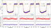 |
Fig. 1. Resulting light curve solutions for the three considered scenarios: β fixed to 0 (left column), β set to 0.25 (middle column), and λ set to −111.59° (right column). The top panels show the observed light curve (orange dots), the observed light curves with the noise removed (blue dots), and the transit model (solid red line). The fitted correlated noise (see text for details) is shown in the middle row, while the residuals where the noise and the transit model are subtracted from the observations are shown in the bottom row (blue dots), with bins of 100 data points (the error bars for the binned points are not shown as they are too narrow). Due to the nature of our analysis, the observed light curve (orange points, top panel) is decomposed into the transit model (solid red line, top panel), the correlated noise (middle panel), and the white noise (blue dots, bottom panel). |
To decide which model describes the system better, we computed the Bayesian and Akaike information criteria (BIC and AIC) for the transit model only (without the noise) as BIC = Nobs ⋅ ln(RSS/Nobs) + Nparams ⋅ lnNobs and AIC = 2 ⋅ Nparams + Nobs ⋅ lnRSS + const., where the constant term is the same for all three scenarios and can thus be disregarded. Here Nobs is the number of measurements used during the fit, Nparams is the number of parameters included in the model, and RSS is the residual sum of squares. Lower BIC and AIC numbers are diagnostic of more plausible models.
The resulting parameter sets for the three cases are shown in Table 1. Almost all parameters, with the obvious exception of the three variables characterizing the gravity darkening (i⋆, λ, and β), are consistent with one another within the estimated uncertainty range. The discrepancies in b between cases (i) and (ii) (β = 0 and β = 0.25) are within 3σ of each other. This means that RP/RS is the only parameter where the fitted values in the two cases are significantly different; similar observations can be made when comparing our findings to the literature (see below). The transit light curve of the first case, where gravity darkening is assumed to be negligible, is a function of seven parameters, while the other two are determined by ten parameters. After calculating the BIC and AIC, we can infer that the β = 0.25 case is the most probable out of the three as ΔBIC = 75.8, ΔAIC = 98.4, ΔBIC = 10.1, and ΔAIC = 10.1, which are lower than in both the β = 0 and λ = −111.59° cases. Thus, we confirm the presence of gravity darkening in the WASP-33b system first noted by Dholakia et al. (2022) and adopt this model.
Parameters derived from the three considered cases.
Comparing the parameters of our adopted model to those from the literature (Table 2), we find good agreements with the no-gravity-darkening model of von Essen et al. (2020) for a/RS, i, P, tC, and (because of the large uncertainty) u−. There is a 3.1σ difference between our fitted value of u+ compared to the same parameter from von Essen et al. (2020), but we note that the authors of that paper used theoretical limb-darkening coefficients. Of more interest is the ratio of the planetary and stellar radii as our value of 0.1098 ± 0.0012 is in good agreement with that of Dholakia et al. (2022) (0.1088 ± 0.0003), but it is significantly different from the 0.1071 ± 0.0002 derived by Herrero et al. (2011). Comparing the results of i⋆, λ, and φ to those from Dholakia et al. (2022), who also fixed the value of the gravity darkening exponent, we find good agreements for the projected and true spin orbit angles, while the stellar inclinations are inconsistent with one another.
Comparison of our derived parameters to the non-gravity-darkened model of von Essen et al. (2020) and the gravity-darkened model of Dholakia et al. (2022) of the same TESS light curve.
The resulting projected spin orbit angle of λ = −94.9° ±21.4° is in good agreement with the retrograde motion discovered by Collier Cameron et al. (2010). However, because of the wide uncertainty range, we were unable to consider the nodal precession observed by, for example, Johnson et al. (2015), Watanabe et al. (2020), and Borsa et al. (2021).
We also note that setting the gravity darkening exponent as a free parameter, as in our case (iii), yields β = 0.58 0.20, which is significantly larger than the nominal value of 0.25. However, it fits in reasonably well with the trend established by Djurašević et al. (2003, 2006).
3.2. Stellar oscillations
The wavelet formulation built into TLCM fits correlated noise simultaneously with the transits, which allowed us to analyze the stellar oscillations without masking the transits. We made use of Period04 (Lenz & Breger 2005) to calculate the spectrum of the identified correlated noise from the adopted solution (where β = 0.25; Fig. 2). Upon visual inspection, this spectrum looks identical to the one published by von Essen et al. (2020). There are peaks in both the δ Sct and γ Dor ranges of the spectrum, which implies that WASP-33 is a γ Dor – δ Sct hybrid pulsator (von Essen et al. 2020).
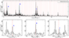 |
Fig. 2. Computed Fourier spectrum (top panel, black), the orbital frequency, and the first 47 orbital harmonics (top panel, dashed red lines) that cover the range of frequencies < 40 days−1, above which no significant peaks are found. The bottom row shows the 3rd, 12th, and 25th orbital harmonics (dashed red lines) and the zoomed-in parts of the spectrum that correspond to these frequencies. |
We identified three pulsational frequencies exceeding S/N > 8 that are very close to one of the orbital harmonics (especially, the 3rd, 12th, and 25th orbital harmonics) in the frequency spectrum. The properties of these peaks are summarized in Table 3. A magnification to the environment of these frequencies and the closest orbital harmonics is shown in the bottom row of Fig. 2. Indeed, the pulsational frequencies are close to the orbital harmonics, and while there is no exact coincidence, the pulsational frequencies are observed to be shifted slightly rightward (toward higher frequencies). The rightward-shifted pulsational frequencies are known as perturbed frequencies, and they are similarly interpreted in the cases of V453 Cyg (Southworth et al. 2020), V1031 Ori (Lee 2021), and RS Cha (Steindl et al. 2021). In these systems, the perturbations have been identified in p modes alone. V453 Cyg, V1031 Ori, and RS Cha are all close binaries with circular orbits that possibly exhibit spin-orbit misalignment, meaning that WASP-33 is a close analog to them. Two of the three frequencies (Fig. 2, bottom row) where the tidal perturbations are the most prominent, near the 12th and 25th orbital harmonics, are likely also pressure-driven modes, which fits in well with the preferred interpretation for this phenomenon. However, Collier Cameron et al. (2010) found from spectroscopic analysis that WASP-33 exhibits g mode pulsations too. As the peak in the Fourier spectrum near the third harmonic is likely caused by g mode oscillations, we suggest that – in the case of WASP-33 only – tidally perturbed oscillations arise in both pressure- and gravity-driven modes as well.
Frequency, amplitude, and S/N of the peaks that are found to be near an orbital harmonic.
In order to investigate the rightward-shifted nature of the pulsational frequencies compared to the orbital harmonics, we created a noise model with the same length as the input light curve, with a Gaussian distribution whose standard deviation is equal to the standard deviation of the residuals of the fitted light curve (∼260 ppm). We injected a sinusoidal signal into this simulated noise model with the same frequency as the orbital harmonic, a randomized phase between 0 and 2π, and an amplitude roughly equal to the height of the respective peaks in the spectrum (340, 440, and 240 ppm). We calculated the Fourier spectrum of the resulting sinusoidal light curve, extracted the frequency of its single peak, and then repeated the process 1000 times. We have found that the widths of the distributions constructed from the bootstrapped frequencies (not shown here) thus determined are negligible compared to the widths of the peaks resulting from the stellar pulsations (Fig. 2, lower row) at 0.0014, 0.0011, and 0.0020 d−1 compared to ∼0.1 d−1. This confirms that the relative positions of the three inspected harmonics compared to the peaks in the spectrum that they correspond to are not caused by a stochastic phenomenon of the particular noise realisation of the original observation.
The distribution of the frequencies in Fig. 2 also suggests that the rightward position of the pulsational frequencies in relation to the closest harmonics of the orbital period may extend to a much larger set of pulsational frequencies than the three most evident examples shown in the lower row of Fig. 2. To examine the position of the stellar frequencies in the “frequency comb” of rotational harmonics, we defined the “fractional frequency” belonging to the stellar modes as
 (2)
(2)
where int represents the integer part of a number. The histogram of the fractional frequencies is shown in the top panel of Fig. 3. The distribution consists of the 17 stellar frequencies with the highest amplitudes. The distribution is very heavy toward the small fractional parts: 13 of 17 frequencies belong to the left half of the distribution ({f/forb}< 0.5), while only 2 stellar frequencies are observed with {f/forb}> 0.6. This asymmetry is not compatible with a stochastic realisation of a uniform distribution. (A uniform distribution would suggest a random set of pulsation frequencies, which are expected if the frequency pattern is not biased, filtered or otherwise modified by the orbital motion of the planet.) We performed a Wilcoxon test (Lupton 1993) to compare the distribution of the observed modular frequencies to a uniform distribution. The p value of the Wilcoxon test measures the probability of having a distribution of a completely random set of numbers “at least as asymmetric” as observed in the spectrum of the stellar signal due only to numerical fluctuations. Thus, if p is small, the observed distribution comes from a uniform distribution with a very low probability. The Wilcoxon p value is plotted in the bottom panel of Fig. 3 as the function of the n number of frequencies included in the test (when the frequencies were sorted according to their amplitude).
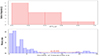 |
Fig. 3. Distribution of the fractional frequencies of the 17 highest amplitude components (upper panel) and the Wilcoxon p values of the fractional part of the n highest amplitude frequencies compared to a uniform distribution (lower panel). |
We find that p < 0.04 in the range of n between 8 and 19. A lower number of frequencies leads to a lack of significance due to the low number statistics, while more frequencies probably include an increasing ratio of the low-amplitude frequencies that are not related to the orbital frequency of the planet.
To reveal the plausibility of mode interactions due to possible hydrodynamical interactions between the modes of stellar pulsation and the tidal forces generated by the planet on the misaligned orbit, we calculated the discrete wavelet transform of the reconstructed stellar signal for frequencies ≤5 d−1, which belong to the first major complex of frequencies toward the long-period end of the frequency distribution (Fig. 2). The wavelet map of this frequency region is shown in Fig. 4. The wavelet map shows vivid amplitude and frequency modulations in the timescale ∼1.5–2 orbits. The degree and the pattern of the detected instability of amplitudes and frequencies in the case of WASP-33 instead suggest a recurrent redistribution of pulsation energy between different modes. Further visual inspection of the wavelet map shows that the oscillations corresponding to the highest two peaks of the bottom-left panel of Fig. 2 (∼2 and ∼2.5 d−1) are not constantly present. It can also be pointed out that the two frequencies are not present simultaneously, and that the oscillations transfer from one mode to the other regularly. This may be caused by star-planet interactions as the stellar spin axis and the orbital plane are not aligned. Due to sampling and smearing, the wavelet transform cannot be used in this analysis at higher frequencies.
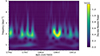 |
Fig. 4. Discrete wavelet map of the identified correlated noise (stellar oscillations plus systematics) in the frequency range 0.5–5 d−1. The gap between ∼1801 and 1804 days is the result of the TESS data downlink. |
We note that Fig. 2 shows the frequency reconstruction with the fixed β = 0.25 parameter during the fit, which belonged to the removal of a transit model with standard gravity darkening before this analysis. We repeated the same analysis as above for the two other planet solutions except as regards the handling of the gravity darkening (no gravity darkening, free β; left and right columns of Fig. 1), and we got practically the same result. Only a slight change in the amplitudes of the peaks can be observed; the frequencies themselves are not affected, and they are always rightward of the closest orbital harmonics.
The process behind this frequency pattern should be more complex than in the case of “heartbeat stars” (e.g., Hambleton et al. 2013, 2016) because in the case of WASP-33 the pattern does not strictly follow the orbital period. But together with the distribution of the fractional frequencies (Fig. 3), this is strong evidence for the tidally perturbed frequency pattern of the host star. It is also different from tidally excited oscillations, as in those cases the eccentric orbits result in a strong coincidence of the orbital harmonics and the peaks in the Fourier spectrum (see, e.g., Fuller 2017; Guo 2021).
4. Summary
We have performed a reanalysis of the light curve of WASP-33 observed by TESS in Sector 18. Our analysis is unique in that we did not perform a pre-whitening of the light curve before modeling the transit. Instead, we used the wavelet formalism built into the TLCM code to fit the stellar pulsations, instrumental noise, and the transit signal of WASP-33b simultaneously.
To test for gravity darkening, we considered three scenarios: no gravity darkening; the gravity darkening exponent, β, fixed to 0.25; and β set as a free parameter of the fit. We have found that the β = 0.25 case describes the light curve best, and thus we confirm the findings of Dholakia et al. (2022).
We also investigated the Fourier spectrum of the stellar oscillations reconstructed by TLCM. There are three peaks in the spectrum (with an S/N > 8) that are at or near an orbital harmonic (3rd, 12th, and 25th). The distribution of the 17 frequencies with the highest amplitudes in relation to the orbital harmonics led us to conclude that the frequencies in the Fourier spectrum tend to be shifted rightward compared to the harmonics. Using a two-sampled Wilcoxon test, we compared their distribution to a uniform distribution of random numbers and found that this rightward-shifted nature is highly unlikely to be caused by a stochastic phenomenon. We suggest that this effect is caused by tidal perturbations of the planetary companion. This would also make WASP-33 the first system where tidal perturbations of the pulsational modes are caused by a substellar companion. The significant changes in frequency and amplitude in the f < 5 days−1 region of the spectrum seen on the wavelet map (Fig. 4) are also diagnostic of planet-star interactions. While the possibility of these interactions has been noted previously by Collier Cameron et al. (2010) and Herrero et al. (2011) (especially at the frequency of 21.311 d−1, a peak altogether missing from our spectrum), our analysis gives detailed, statistical proofs of the stellar oscillations caused by tidal forces. We also suggest that the misalignment of the stellar rotational axis and the planetary orbit is causing the perturbations of the stellar pulsational modes.
The data are available from the Mikulski Archive for Space Telescopes: https://mast.stsci.edu/portal/Mashup/Clients/Mast/Portal.html
Acknowledgments
We acknowledge the support of the Hungarian National Research, Development and Innovation Office (NKFIH) grant K-125015, a PRODEX Experiment Agreement No. 4000137122, the Lendület LP2018-7/2021 grant of the Hungarian Academy of Science and the support of the city of Szombathely. Prepared with the professional support of the Doctoral Student Scholarship Program of the Cooperative Doctoral Program of the Ministry of Innovation and Technology financed from the National Research, Development and Innovation Fund.
References
- Barnes, J. W. 2009, ApJ, 705, 683 [Google Scholar]
- Benz, W., Broeg, C., Fortier, A., et al. 2021, Exp. Astron., 51, 109 [Google Scholar]
- Borsa, F., Lanza, A. F., Raspantini, I., et al. 2021, A&A, 653, A104 [NASA ADS] [CrossRef] [EDP Sciences] [Google Scholar]
- Borucki, W. J., Koch, D., Basri, G., et al. 2010, Science, 327, 977 [Google Scholar]
- Carter, J. A., & Winn, J. N. 2009, ApJ, 704, 51 [Google Scholar]
- Chakrabarty, A., & Sengupta, S. 2019, AJ, 158, 39 [NASA ADS] [CrossRef] [Google Scholar]
- Christian, D. J., Pollacco, D. L., Skillen, I., et al. 2006, MNRAS, 372, 1117 [NASA ADS] [CrossRef] [Google Scholar]
- Collier Cameron, A., Guenther, E., Smalley, B., et al. 2010, MNRAS, 407, 507 [NASA ADS] [CrossRef] [Google Scholar]
- Csizmadia, S. 2020, MNRAS, 496, 4442 [Google Scholar]
- Csizmadia, S., Smith, A. M. S., Cabrera, J., et al. 2021, A&A, submitted, [arXiv:2108.11822] [Google Scholar]
- Dholakia, S., Luger, R., & Dholakia, S. 2022, ApJ, 925, 185 [NASA ADS] [CrossRef] [Google Scholar]
- Djurašević, G., Rovithis-Livaniou, H., Rovithis, P., et al. 2003, A&A, 402, 667 [NASA ADS] [CrossRef] [EDP Sciences] [Google Scholar]
- Djurašević, G., Rovithis-Livaniou, H., Rovithis, P., et al. 2006, A&A, 445, 291 [NASA ADS] [CrossRef] [EDP Sciences] [Google Scholar]
- Fabrycky, D. C., & Winn, J. N. 2009, ApJ, 696, 1230 [NASA ADS] [CrossRef] [Google Scholar]
- Fuller, J. 2017, MNRAS, 472, 1538 [Google Scholar]
- Guo, Z. 2021, Front. Astron. Space Sci., 8, 67 [NASA ADS] [Google Scholar]
- Hambleton, K. M., Kurtz, D. W., Prša, A., et al. 2013, MNRAS, 434, 925 [Google Scholar]
- Hambleton, K., Kurtz, D. W., Prša, A., et al. 2016, MNRAS, 463, 1199 [Google Scholar]
- Herrero, E., Morales, J. C., Ribas, I., & Naves, R. 2011, A&A, 526, L10 [NASA ADS] [CrossRef] [EDP Sciences] [Google Scholar]
- Hey, D. R., Montet, B. T., Pope, B. J. S., Murphy, S. J., & Bedding, T. R. 2021, AJ, 162, 204 [NASA ADS] [CrossRef] [Google Scholar]
- Johnson, M. C., Cochran, W. D., Collier Cameron, A., & Bayliss, D. 2015, ApJ, 810, L23 [Google Scholar]
- Kálmán, Sz., Szabó, Gy. M., & Csizmadia, Sz. 2021, A&A, submitted [Google Scholar]
- Lee, J. W. 2021, PASJ, 73, 809 [NASA ADS] [CrossRef] [Google Scholar]
- Lenz, P., & Breger, M. 2005, Commun. Asteroseismol., 146, 53 [Google Scholar]
- Lightkurve Collaboration (Cardoso, J. V. d. M., et al.) 2018, Lightkurve: Kepler and TESS time series analysis in Python (Astrophysics Source Code Library) [Google Scholar]
- Lupton, R. 1993, Statistics in Theory and Practice (Princeton, N.J: Princeton University Press) [Google Scholar]
- Mandel, K., & Agol, E. 2002, ApJ, 580, L171 [Google Scholar]
- Ricker, G. R., Winn, J. N., Vanderspek, R., et al. 2015, J. Astron. Telesc. Instrum. Syst., 1, 014003 [Google Scholar]
- Southworth, J., Bowman, D. M., Tkachenko, A., & Pavlovski, K. 2020, MNRAS, 497, L19 [Google Scholar]
- Stassun, K. G., Oelkers, R. J., Paegert, M., et al. 2019, AJ, 158, 138 [Google Scholar]
- Steindl, T., Zwintz, K., & Bowman, D. M. 2021, A&A, 645, A119 [NASA ADS] [CrossRef] [EDP Sciences] [Google Scholar]
- von Essen, C., Czesla, S., Wolter, U., et al. 2014, A&A, 561, A48 [NASA ADS] [CrossRef] [EDP Sciences] [Google Scholar]
- von Essen, C., Mallonn, M., Borre, C. C., et al. 2020, A&A, 639, A34 [NASA ADS] [CrossRef] [EDP Sciences] [Google Scholar]
- von Zeipel, H. 1924, MNRAS, 84, 684 [NASA ADS] [CrossRef] [Google Scholar]
- Watanabe, N., Narita, N., & Johnson, M. C. 2020, PASJ, 72, 19 [CrossRef] [Google Scholar]
All Tables
Comparison of our derived parameters to the non-gravity-darkened model of von Essen et al. (2020) and the gravity-darkened model of Dholakia et al. (2022) of the same TESS light curve.
Frequency, amplitude, and S/N of the peaks that are found to be near an orbital harmonic.
All Figures
|
Fig. 1. Resulting light curve solutions for the three considered scenarios: β fixed to 0 (left column), β set to 0.25 (middle column), and λ set to −111.59° (right column). The top panels show the observed light curve (orange dots), the observed light curves with the noise removed (blue dots), and the transit model (solid red line). The fitted correlated noise (see text for details) is shown in the middle row, while the residuals where the noise and the transit model are subtracted from the observations are shown in the bottom row (blue dots), with bins of 100 data points (the error bars for the binned points are not shown as they are too narrow). Due to the nature of our analysis, the observed light curve (orange points, top panel) is decomposed into the transit model (solid red line, top panel), the correlated noise (middle panel), and the white noise (blue dots, bottom panel). |
| In the text | |
|
Fig. 2. Computed Fourier spectrum (top panel, black), the orbital frequency, and the first 47 orbital harmonics (top panel, dashed red lines) that cover the range of frequencies < 40 days−1, above which no significant peaks are found. The bottom row shows the 3rd, 12th, and 25th orbital harmonics (dashed red lines) and the zoomed-in parts of the spectrum that correspond to these frequencies. |
| In the text | |
|
Fig. 3. Distribution of the fractional frequencies of the 17 highest amplitude components (upper panel) and the Wilcoxon p values of the fractional part of the n highest amplitude frequencies compared to a uniform distribution (lower panel). |
| In the text | |
|
Fig. 4. Discrete wavelet map of the identified correlated noise (stellar oscillations plus systematics) in the frequency range 0.5–5 d−1. The gap between ∼1801 and 1804 days is the result of the TESS data downlink. |
| In the text | |
Current usage metrics show cumulative count of Article Views (full-text article views including HTML views, PDF and ePub downloads, according to the available data) and Abstracts Views on Vision4Press platform.
Data correspond to usage on the plateform after 2015. The current usage metrics is available 48-96 hours after online publication and is updated daily on week days.
Initial download of the metrics may take a while.