| Issue |
A&A
Volume 659, March 2022
|
|
|---|---|---|
| Article Number | A58 | |
| Number of page(s) | 12 | |
| Section | The Sun and the Heliosphere | |
| DOI | https://doi.org/10.1051/0004-6361/202142346 | |
| Published online | 07 March 2022 | |
Physical properties of a fan-shaped jet backlit by an X9.3 flare
Institute for Solar Physics, Dept. of Astronomy, Stockholm University, Albanova University Centre, 106 91 Stockholm, Sweden
e-mail: This email address is being protected from spambots. You need JavaScript enabled to view it.
Received:
1
October
2021
Accepted:
23
November
2021
Abstract
Context. Fan-shaped jets sometimes form above light bridges and are believed to be driven by the reconnection of the vertical umbral field with the more horizontal field above the light bridges. Because these jets are not fully opaque in the wings of most chromospheric lines, it is not possible to study their spectra without highly complex considerations of radiative transfer in spectral lines from the atmosphere behind the fan.
Aims. We take advantage of a unique set of observations of the Hα line along with the Ca II 8542 Å and Ca II K lines obtained with the CRISP and CHROMIS instrument of the Swedish 1-m Solar Telescope to study the physical properties of a fan-shaped jet that was backlit by an X9.3 flare. For what we believe to be the first time, we report an observationally derived estimate of the mass and density of material in a fan-shaped jet.
Methods. The Hα flare ribbon emission profiles from behind the fan are highly broadened and flattened, allowing us to investigate the fan with a single slab via Beckers’ cloud model, as if it were backlit by a flat spectral profile of continuum emission. Using this model we derived the opacity and velocity of the material in the jet. Using inversions of Ca II 8542 Å emission via the STockholm inversion Code, we were also able to estimate the temperature and to cross-check the velocity of the material in the jet. Finally, we used the masses and the plane-of-sky and line-of-sight velocities as functions of time to investigate the downward supply of energy and momentum to the photosphere in the collapse of this jet, and evaluated it as a potential driver for a sunquake beneath.
Results. We find that the physical properties of the fan material are reasonably chromospheric in nature, with a temperature of 7050 ± 250 K and a mean density of 2 ± 0.3 × 10⁻¹¹ g cm−3.
Conclusions. The total mass observed in Hα was found to be 3.9 ± 0.7 × 10¹³ g and the kinetic energy delivered to the base of the fan in its collapse was nearly two orders of magnitude below typical sunquake energies. We therefore rule out this jet as the sunquake driver, but cannot completely rule out larger fan jets as potential drivers.
Key words: sunspots / Sun: flares / Sun: atmosphere / Sun: chromosphere / methods: observational / line: formation
© ESO 2022
1. Introduction
Hα surges were first reported in McMath & Pettit (1937), where they were classified as class IIId prominences. Since then surges have been a point of interest for ongoing solar research (e.g., Newton 1942; Ellison 1949; Malville & Moreton 1961; Schmieder et al. 1994; Uddin et al. 2012; Robustini et al. 2018; Nóbrega Siverio et al. 2021).
These structures are described as straight or slightly curved spikes of cool material (< 15 kK) that appear most often in absorption in chromospheric lines such as Hα and Ca II 8542 Å on the solar disk (Bruzek & Durrant 1977). They originate from small bright points close to sunspots and pores, and are believed to be the result of reconnection events between newly emerging flux and a pre-existing magnetic field (e.g., Yokoyama & Shibata 1995; Kayshap et al. 2013; Robustini et al. 2016). However, it has also been shown that they can be triggered by the impulsive generation of a pressure pulse (Sterling et al. 1993), and can be associated with explosive events (Madjarska et al. 2009). Typical lifetimes for surges are between 10 and 20 min, but longer-lived surges of over 40 min and even over an hour have been reported (e.g., Robustini et al. 2018; Kayshap et al. 2021). Jets studied by Roy (1973a,b,c) reached heights between 7 and 50 Mm, but much higher jets up to 200 Mm have been reported (e.g., Bruzek & Durrant 1977; Louis & Thalmann 2021). The material that is propelled upward in surges is thought principally to return approximately along the trajectory of ascent, with some small fraction possibly being heated to coronal values and remaining at higher locations in the solar atmosphere (Robustini et al. 2016, 2018). In Roy (1973c) it was reported that the material in surges accelerated more slowly than the effective gravity (the solar gravitational component along the trajectory of ascent and descent), suggesting the presence of a breaking force. However this effect was not found in more recent work by Robustini et al. (2016), where the acceleration was found to be consistent with effective solar gravity.
Bruzek & Durrant (1977) suggest that the magnetic field strength inside surges is around 50 G and decreases with height, which is consistent with those reported by Harvey (1969), who measured field strengths between 17 and 87 G in surges on the limb. A more recent estimate was made by Yoshimura et al. (2003), who suggested a field strength between 100 and 300 G based on an estimate of the reconnection energy. The models of Ding et al. (2010) produced still lower field strength values, between 6 and 40 G. Ding et al. (2010) found that in their models the jet temperature depended on the magnetic field strength and the jet density. A jet with a weak magnetic field (6 G) and high density showed lower, more chromospheric temperatures (≈104 K), while a jet with a higher magnetic field (40 G) and lower density would result in a hot surge with much higher temperatures (around 6 × 10⁵ K). Simulations producing “hot surges” have also been reported (e.g., Nishizuka et al. 2008; Kayshap et al. 2013). Hot surge simulation results have been challenged more recently in Nóbrega-Siverio et al. (2016), who suggest that hot surges will likely cool down rapidly to ≈104 K when detailed radiative losses are considered. A surge with lower temperature have also been reported more recently, with observed brightness temperature of 5.5 kK by Robustini et al. (2016).
Fan-shaped jets, or peacock jets, are a subclass of surges that appear over light bridges. This was first reported by Roy (1973b,c) and studied as an independent phenomenon by Asai et al. (2001), where the jets were described as recurring jets that appear dark in Hα, and also visible in the extreme ultraviolet. A measurement of the line-of-sight (LOS) magnetic field by Bharti et al. (2007) shows that some of these jets can have a polarity opposite to that of the umbral field. Small jets up to 13 Mm were reported by Shimizu (2009) and Shimizu et al. (2009), and much smaller jets, most no longer than 1000 km, by Louis et al. (2014).
Due to the complexity of the 3D radiative transfer problem and the highly variable background around sunspots, the inference of detailed physical parameters of the fan jets from inversions of the convolved spectra they produce in front of their backgrounds has so far proven to be an intractable task. This has limited many of the results that were presented above, especially with respect to temperature and density. As a result, there are no observationally constrained density measurements of surges, and typical chromospheric values are often assumed for simulations. An estimate of the mass and density of a large surge was made by Roy (1973c) based solely on an isotropic expansion of chromospheric material from the base of the fan, giving values for mass on the order of 1015 and 1016 g, and for density of 1011 and 1012 particles cm−3. In this paper we present a unique dataset that allows us to make what we believe is the first observationally constrained mass and density measurement of a fan-shaped jet. We also estimate the amount of returning mass that hits the base of the fan as a function of time. This in turn allows us to explore the potential of surges as a trigger for sunquakes1 by comparing the downward delivered momentum and energy budgets of material in the jet to that of measured sunquakes. We do not attempt to infer the magnetic field of the jet, given that these fields are weaker by several orders of magnitude than those of a flare (e.g., Vissers et al. 2021).
In Sect. 2 we discuss our observations, the reduction, and the spectral profiles found within the fan-jet. In Sect. 3 we discuss our models and the assumptions that allowed us to use these models. The results from our inversions are shown and discussed in Sect. 4. Our final conclusions can be found in Sect. 5.
2. Observations and data processing
Region AR 12673 was observed on 6 September, 2017, between 11:55 and 12:52 UT, with the Swedish Solar 1-m Telescope (SST, Scharmer et al. 2003), using simultaneously the CRisp Imaging SpectroPolarimeter (CRISP, Scharmer et al. 2008) and the CHROMospheric Imaging Spectrometer (CHROMIS; Scharmer 2017). The region was centered around the heliocentric coordinates (x, y) = (537″, −222″), which translates to an observing angle of 37° (μ = 0.79). A sequence was run on CRISP that alternated between Hα and Ca II 8542 Å, while on CHROMIS only the Ca II K line was observed. This dataset was first described in detail in Quinn et al. (2019), although the CHROMIS Ca II K data are reduced for the first time in the present paper; the Ca II K 4000 Å continuum point is employed for context images and to identify the location of the base of the fan jet that we investigated for this paper. In the relevant time frames the Ca II K line profiles did not have good enough seeing quality to significantly contribute to this project.
For CRISP the cadence was 15 s and the observing sequence consisted of 13 wavelength positions in the Hα line, at ±1.5, ±1.0, ±0.8, ±0.6, ±0.3, ±0.15, and 0 Å relative to line center. The Ca II 8542 Å scan consisted of 11 wavelength positions taken in full-Stokes polarimetry mode at ±0.7, ±0.5, ±0.3, ±0.2, ±0.1, and 0 Å relative to line center. The CRISP pixel scale is 0.058″.
For CHROMIS the cadence of the observing sequence was 6.5 s with 10 wavelength positions in the Ca II K line at ±1.00, ±0.85, ±0.65, ±0.55, ±0.45, ±0.35, ±0.25, ±0.15, ±0.07, and 0.00 Å relative to line center, plus a single continuum point at 4000 Å. The CHROMIS pixel scale is 0.0375″. In addition to the narrowband images, wideband images were also obtained co-temporally with each CRISP and CHROMIS narrowband exposure to be used for alignment purposes.
2.1. Data processing
Both datasets were reduced using the SSTRED pipeline, as described by de la Cruz Rodríguez et al. (2015) and Löfdahl et al. (2021), which makes use of Multi-Object Multi-Frame Blind Deconvolution (MOMFBD; Löfdahl 2002; van Noort et al. 2005). Additionally, we performed an absolute wavelength and intensity calibration using the solar atlas by Neckel & Labs (1984).
We extensively used the CRISPEX analysis tool (Vissers 2012); COCOPLOTs (Druett et al. 2021a); SOAImageDS9 (Joye & Mandel 2003); and the CRISpy python package (Pietrow 2019), which is now part of the ISPy library (Diaz Baso et al. 2021) for data visualization during the preparation of this article.
2.2. Field of view
In Fig. 1 we give an overview of the field of view (FoV). In the 4000 Å continuum (panel a) we see a large delta sunspot crossed by a light bridge at (x, y) = 12″, 20″ arcsec. In the chromospheric lines (panels b–d) we see a pair of large flare ribbons belonging to the X9.3 flare that appear bright in all three panels, and that expand outward over time. In front of the eastern flare ribbon (left), at (x, y) = 15″, 20″ arcsec a fan jet rooted above the light bridge appears as a dark feature against the bright flare ribbon in all the chromospheric filters. This structure is most clearly seen in the Hα line. We indicate the region containing this feature in each of the frames (white dotted rectangle) and enlarged it in panel e. This area is the FoV used in this article to study the jet. With an apparent maximum extent of roughly 6 Mm in Ca II 8542 Å, this jet is very small compared with those typically studied in the literature. We arrive at the estimate of 6 Mm using the apparent deprojected locations of the footpoint of the structure seen in the coaligned Ca II K 4000 Å continuum point and the head of the jet observed in Ca II 8542 Å.
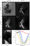 |
Fig. 1. Overview of AR 12673 taken on 6 September 2017 at 11:59 UT. The fan jet is indicated by a white rectangle. Panel a: continuum intensity 4000 Å; b: Ca II 8542 Å line core intensity; c: Ca II K line core intensity; d: Hα line core intensity; e: enlarged view of white rectangle in panel d. The red, blue, green, and orange dots show the physical locations from which the profiles shown in panel f were taken; f: Hα profiles of flare ribbon (red) and fan jet (blue, green, yellow). |
In order to summarize the pattern of Hα profiles observed in this region, four locations have been selected from the data at points shown by the colored dots in panel e. The corresponding Hα profiles are shown in panel f, using the same colors. The background flare ribbon (red), contains spectral profiles that have similar intensities across the entire wavelength window. This results from line broadening in flares that has been observed to extend up to 5 Å from the line center (e.g., Ichimoto & Kurokawa 1984; Wuelser & Marti 1989; Zarro et al. 1988). Highly broadened profiles in this flare are also presented in Zharkov et al. (2020) and Zharkova et al. (2020). Profiles taken from locations where the fan jet is visible (blue, green, and yellow) show background levels consistent with the flare ribbon emission in the far wings, and with absorption features caused by the material in the fan jet elsewhere. Profiles taken more toward the center of the fan generally show broader absorption profiles with more flattened cores. In this paper we focus primarily on the Hα data, using the Ca II 8542 Å only to obtain an estimate of the fan temperature.
As the flare ribbon expands it reaches the base of the fan jet (at the location of the light bridge) and the fan begins collapsing. This suggests that the flare ribbon is suppressing the flows of material upward from its base. The collapse of the fan jet is shown in Fig. 2, between 11:59 and 12:01 UT. The images in the time series are consistent with the jet being oriented approximately perpendicularly to the solar surface. This statement is based on comparing the angle that would be derived from the observing angle (37°) to the viewing angles calculated by using LOS and plane-of-sky (POS) velocities of fan material (which had a mean value of 44° over the “spines” of the fan; see Sect. 3.3). This study focuses only on the collapse of the fan jet to estimate its mass, due to poorer seeing in the time frames before the collapse began. From the LOS velocities and the visible top of the jet, we infer that the jet collapses from the second frame of Fig. 2, since its structure remains nearly identical in the first two frames. This suggests that we have reasonable seeing from the start of the collapse of the fan in our limited time series. A qualitative representation of the physical situation of the observations can be seen in Fig. 3.
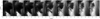 |
Fig. 2. Time series of fan jet from 11:59 UT to 12:01 UT with 15 s between each panel. |
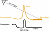 |
Fig. 3. Cartoon showing a simplified side-on view of the physical situation being studied at two optical depth values for the photosphere and chromosphere. A fan jet is situated above a light bridge with a hot flare ribbon behind it. From our perspective the fan is backlit by the ribbon. |
3. Data inversions
3.1. Beckers’ cloud model
We performed inversions of the Hα profiles from the selected FoV by using Beckers’ cloud model (BCM, Beckers 1964). This is a solution to the radiative transfer equation for an atmosphere with a “slab” or “cloud” of material above it. In this model the cloud absorbs radiation coming from behind it. The optical depths can then be derived from the model by the absorption profiles that are superimposed on the background (Tziotziou 2007). In our model the background is the flare ribbon emission and the cloud is the material in the fan jet (see Fig. 3).
In order to solve the radiative transfer equation, Beckers made several assumptions for this model. First, he assumed that the slab is fully separated from the underlying atmosphere (equivalent to the assumption that the material in the fan jet is spatially separated from the material in the flare ribbon) behind it in the LOS. Second, he assumed that the slab is homogeneous along the LOS, meaning that the inferred parameters are also constant along the LOS. This assumption will not be strictly satisfied for the material in the fan jet, but should be sufficient to provide an estimate of the material in the fan jet in each pixel in the FoV. Finally, the BCM requires the background intensity to be known. Additionally, in this unique setup of a fan jet that is backlit by a flare, the highly broadened and flattened Hα emission profiles from the flare ribbon allow us to approximate the fan jet as if it were backlit by continuum emission (Figs. 1f and 3, red line). One objection to this approximation is that the flare ribbon profiles could be strongly peaked outside of the spectral window. However, due to the differences in wavelength, peaks in the full Hα emission profiles that occur outside of the spectral window, like those observed in Wuelser & Marti (1989), will have very low probabilities of interacting with the absorption in Hα resulting from the material in the fan. The assumption that the flare ribbon emissions are similar behind the fan to those in the area surrounding it is corroborated by the similar blue wing intensities (e.g., the curves in Fig. 1f at −1.5 Å), and also the similar flattened flare profiles seen simultaneously in all regions of the main flare ribbon around the fan.
Under these assumptions the radiative transfer equation simplifies to
 (1)
(1)
where I(Δλ) is the observed intensity, I0(Δλ) the background intensity, τ(Δλ) the optical depth, and S the source function of the cloud material. Typically these models assume either a Gaussian or Voigt profile for the absorption profiles as a function of wavelength, which then gives a similar profile over wavelength in optical depth (Tsiropoula 1999). For our study we selected the more general Voigt profile. Our model uses the lmfit Python package (Newville et al. 2014) along with the Bound Limited memory Broyden-Fletcher-Goldfarb-Shanno algorithm (L-BFGS-B Byrd et al. 1995) to minimize the residuals between observed input profile and synthetic spectra in an iterative manner.
The code treats each pixel separately; that is to say, their corresponding profiles are fitted independently from each other. A second fit was made to the same profiles, excluding the outermost wavelength points in order to obtain better fits to the profiles with stronger asymmetries in the far wings. These values are used to replace results from the first fit where the residuals were greater than 0.8. We illustrate the difference between the two fits in Fig. 4, where we see a symmetrical profile that the cloud model easily reproduces in its entirety, while a profile that has asymmetrical far wings was more dubiously fitted. Neglecting the two outermost points allowed us to accurately fit the main curve of the absorption profile, and hence provide a more conservative estimate of the optical depth for the main component of the material in the fan jet (see Fig. 4, lower panel, blue line).
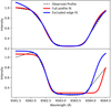 |
Fig. 4. Plot of examples of Hα profiles from pixels containing the fan jet (black) and the fit using the BCM including (red) and excluding (blue) the two outermost wavelength points. Top: fitted profile with a low χ2, showing good agreement between the blue and red curves. Bottom: profile with asymmetrical far wings that caused a high χ2 value in the original fit, and a much better fit to the main component shown by the blue curve. |
In order to select the pixels that we were confident contained material in the fan jet, we only selected profiles with an absorption feature. This was achieved by requiring the quotient of the lowest intensity across all the wavelength points to the intensity in the central wavelength point to be 0.8 or higher. The resulting mask of selected pixels was then manually checked, and anomalous pixels were removed to form a final mask for each time frame. This means that an area smaller than that of the full fan is used during our inversions, resulting in an influence toward underestimation of the total optical depth and mass contained.
Using this model we inverted our Hα time series, fitting for the following parameters: the optical depth of the line core τ0, the Doppler shift, the damping parameter of the Voigt function Γ, the Gaussian width of the Voigt function σ (which includes Doppler broadening, microturbulence, and other effects), I0, and S0. All values except the Doppler shift were bounded to be positive. The values of I0 and S0 were assumed to be constant along the wavelength range, with their initial guesses inferred from the profile minimum and maximum.
To reproduce the widths of these profiles a great deal of broadening was required. This implies some combination of high Gaussian broadening (i.e., increased σ via high temperatures or microturbulent velocities) and additional effects such as Lorentzian broadening, velocity gradients within the formation region, or optically thick line formation effects, such as opacity broadening (see Molnar et al. 2019).
The study of Cauzzi et al. (2009) using cloud modeling for Hα required adjustments equivalent to temperatures of up to 60 kK to fit their profiles. Additionally, Tziotziou et al. (2007) found that the Hα line widths in quiet Sun observations were strongly affected by the seeing and by the fact that the retrieved optical depth values are negatively skewed, once again resulting in an influence toward some large underestimations of optical depths and therefore the total mass contained in the fan jet.
Modeling the broadening principally by using higher τ0 values does not result in good fits of the full profiles; the opacity broadening principally results in saturation of the intensity profile in the core to the source function values of the cloud at high opacity, meaning that a broader profile will also have a flatter core. This saturation happens for a greater span of wavelengths in the absorption profile as τ0 increases significantly above unity. However, this fitting via higher optical depth is particularly poor in the line wings, which become much steeper than in the observations, and thus result in large values of χ2. The vast majority of the profiles are symmetrical, and thus the widths of these profiles are unlikely to be the result of strong velocity gradients. If they were, this would imply that very particular patterns of velocity gradients that happen to result in symmetrical profiles are present in the majority of pixels, across the FoV, and for different angles of orientation between the fan spines and the viewer. A small fraction of profiles show some asymmetries that would be better explained using this information, but these profiles have a main absorption feature in line with the widths of profiles in the surrounding features, and an additional element that likely represents a feature created by a strong velocity gradient. In the small number of more asymmetrical profiles our routine focuses on fitting what appears to be the main absorption feature of the profile (see Fig. 4). The best fits produced a close match to both the absorption core and the gradients of the wings. This was achieved by the algorithm in almost every case by using lower but still optically thick τ values coupled with substantial broadening of the Gaussian width parameter σ. Asymmetric profile features resulting from velocity gradients are commonly observed in flares but can also be found in quiet Sun features as well, and have been investigated in numerous studies (e.g., Kuridze et al. 2015; Druett et al. 2017; Capparelli et al. 2017; Druett & Zharkova 2018). For example, in our data we see a “horn” of the Hα profile in the blue wing or a lower gradient away from the central Doppler shifted component in the red wing, which are both visible in the lower panel of Fig. 4 (black line).
This high σ value for Hα remains unexplained and may imply high turbulent broadening or temperatures. This is certainly worthy of detailed investigation that is not within the remit of this paper. We infer temperature by other, more reliable methods using a different spectral line (see Sect. 3.2) and use this cloud model to focus only on the τ0 and Doppler shift. We conjecture that due to expected temperature estimates obtained via other spectral lines, that if σ is indeed large, there must be significant microturbulent broadening in Hα. However, due to the non-degenerate χ2 values for our fits of the Hα line, we remain reasonably confident of the estimates of τ0 inferred. This kind of large-scale Hα broadening is also present in flares, and is as-yet-unexplained phenomenon that we took advantage of by assuming a flat profile of continuum-like backlighting.
Once we had an estimate of τ0 for each pixel in our fan, we converted this optical depth into a column mass using the relation found in Leenaarts et al. (2012), where the authors showed that the Hα line optical depth loses sensitivity to variations of temperature under chromospheric conditions (i.e., variations within typical chromospheric temperatures that are sufficiently above that of the temperature minimum region, but below the ionization temperature of hydrogen). The opacity becomes mainly determined by the mass density, which in turn implies that the optical depth is proportional to the column mass. We use this proportionality in our work to convert the optical depth directly into a column mass (m [g cm−3] = 3 × 10⁻⁵ × τ0). The column mass per pixel is equal to the total observed mass in the fan jet per pixel in our case as the absorption is caused by the cloud only.
If we assume a uniform thickness for the fan in the LOS, it is also possible to translate the mass estimate into a density estimate, by dividing the column mass by the thickness of the fan jet in the LOS. A thickness estimate of the fan was obtained by looking at the narrowest width of an individual fan structure that was resolved in the images, and estimated at around 200 km, which matches the typical width of a narrow fibrillar structure (Kianfar et al. 2020; Zhou et al. 2020). Then our density figures can be compared to those of similar observed phenomena, and potentially to simulations at a later stage. We can use this density estimate to create a second cloud model that fits the fan’s Ca II 8542 Å profiles, as described in the following section.
This choice for thickness is likely to be an underestimate as it supposes that the narrowest observed feature is suitable for use as the general estimate for the thickness of the fan. There is a direct relationship between the thickness and the resulting densities that are derived from our estimate of the mass, specifically that we could choose a greater thickness and thus obtain lower densities. However, in the following section we found that our model is not able to reproduce the Ca II 8542 Å spectral profile as successfully when using a thickness for the slab that is larger by a factor greater than two without also requiring higher density values. We note that the assumptions made in calculating the mass estimate of the fan jet lead to a result that is a lower limit, whereas the subsequent assumption made for the thickness of the fan influences the estimates of densities toward greater values, and thus cannot be considered formally as either an upper or a lower limit.
3.2. Temperature fitting
In order to estimate the temperatures of the flare and the fan jet (and thus to corroborate our prior assumption that the temperature in the fan jet is chromospheric at the beginning of the collapse) we constructed a second cloud model. This model employs the STockholm inversion Code (STiC) to perform inversions of the reduced Ca II 8542 Å profiles from the selected FoV. The profiles in Ca II 8542 Å from the fan jet and nearby flare ribbon were not broadened greatly by unexplained processes at the time of the fan collapse (unlike in Hα) and were also resolved within the wavelength window of the observations. Therefore, it would not have been reliable to use the BCM with an approximation of a flat continuum background in Ca II 8542 Å, nor would it have been reliable to fit any other background profile without taking into account spatial dependence. In the method described below we restrict ourselves to comparing the flare and fan jet information in spatially close locations, near to the edge of the jet to maximize the likelihood of similarity in the background emission profiles from the flare (see Fig. 8c).
STiC2 (de la Cruz Rodríguez et al. 2016, 2019) is a message passing interface parallel (MPI-parallel), non-local thermodynamic equilibrium (NLTE) inversion code that utilizes a modified version of the RH code (Uitenbroek 2001) to solve the atom population densities assuming statistical equilibrium and plane-parallel geometry. The radiative transport equation is solved using cubic Bezier solvers (de la Cruz Rodríguez & Piskunov 2013). The inversion engine of STiC includes an equation of state extracted from the SME code (Piskunov & Valenti 2017). STiC uses a regularized version of the Levenberg-Marquardt algorithm (Levenberg 1944; Marquardt 1963) to iteratively minimize the χ2 function between observed input data and synthetic spectra of one or more lines simultaneously. The code treats each pixel separately as a plane-parallel atmosphere, fitting them independently of each other.
Using STiC we invert representative Ca II 8542 Å profiles of the flare ribbon to obtain a model atmosphere for the background3. A uniform slab with a thickness of 200 km, representing the fan jet, is inserted at the upper boundary of the atmosphere above the flare ribbon atmosphere derived from the first step. We choose to put the slab on top because the slab if is introduced at the upper boundary in a density and temperature regime where the Ca II 8542 is otherwise not sensitive, it does not affect the background atmosphere. Unlike the slab model used to estimate the mass density, this slab is introduced in a depth-stratified atmosphere by setting the upper 200 km of the atmospheric model with constant values of T, vlos, vturb, and the estimated mass density. The slab gently transitions to the pre-existing parameter stratification over a span of three grid points below the top 200 km. This is done for numerical reasons. When STiC solves the NLTE problem, changes in LOS velocity between grid points that are larger than half the Doppler width of the line will induce errors in the intensities.
To estimate the values of the parameters in the slab, STiC is only used as a forward modeling synthesis tool to compare the resulting profile with the observations, and the inversion is done by the Levenberg-Marquardt algorithm. We do not consider hydrostatic equilibrium in this experiment, and thus turned it off for these inversions.
The profile from the fan jet was fitted using the parameter space of the slab (T, vlos, and vturb) via a Levenberg-Marquardt minimization routine4 (de la Cruz Rodríguez et al. 2019), while keeping the rest of the model stratification fixed, in a way similar to that described in Díaz Baso et al. (2019).
We repeated this inversion, varying the slab thickness with values from 100 km up to 800 km, and using proportionally scaled densities. For values of the slab thickness from 200 km to 400 km there was a degeneracy between the density and thickness, and we were able to achieve similar quality fits with these degenerate values. However, the final χ2 values of the fits were higher for larger values for the fan thickness, and more dramatically so above 400 km and below 200 km. For this reason we continue our investigation by assuming a slab thickness of 200 km.
Regardless of these variations, we derived similar slab temperatures, all within the uncertainty in Sect. 4.5, for each of the inversions that were able to fit the observed profile. Therefore, we believe that while there may be some degeneracy in our inferred densities and slab thickness, a robust value for the temperature of the slab is derived (see Fig. 5).
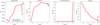 |
Fig. 5. Stratification in geometrical height scale of parameters (T, vlos, vturb) inverted with our second cloud model (described in Sect. 3.2) as well as the inferred density from the first cloud model (described in Sect. 3.1). The black line shows the stratification of these parameters for the flare ribbon background, while the red line compares these same parameters for the best fit of an inverted pixel inside of the fan. Note that the model stratification is fixed everywhere except in the slab at the top of the atmosphere. Panel a: temperature; panel b: LOS velocity; panel c: microtubulence; and panel d: density. The observed and best-fit profiles belonging to these atmospheres can be found in Fig. 8c. |
3.3. Collapse velocities and acceleration
We obtained velocity estimates for the collapse of the fan jet by combining measurements of the LOS and POS velocities. The latter was found by tracking the top of the fan jet along six trajectories, or fan “spines”, which were aligned with visible structure within the fan (see Fig. 6a) during the first six frames of the collapse. The values became unreliable for the later frames of the time series because large parts of the fan lost visibility in Hα, likely due to energy from radiation and heating that was ionizing the neutral hydrogen (see Fig. 2). The top of the fan on each spine is found from the fact that the BCM breaks down on the edge; at this point there ceases to be a clear absorption profile and the fitting routine attempts to interpret the resulting asymmetric line profile via a single Voigtian profile. This generally produces a high Doppler shift causing a strong peak in the LOS velocity parameter at the point where, moving upward along the spine, you reach the top of the fan, before dropping to 0 km s−1 outside of it because the emission (flare ribbon) or absorption (off ribbon) line profiles are generally centered on the rest wavelength. This can be seen on the right side of each profile in Fig. 6b, and the collapsing top of the fan can be tracked along this spine by noting the change in position of this peak over time. We illustrate the collapse of the fourth spine in Fig. 6b by plotting the vlos along this spine in the first six time frames. This spine was chosen for its central location inside the fan, which had a clear dark appearance and was less susceptible to ionization over the time frames considered. The collapse can be inferred from the position of the peak in LOS velocity on the right side of each profile in this panel.
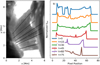 |
Fig. 6. Collapse of the fan tracked along six spines. Panel a: minimum value of the Hα emission intensity. This shows the fan in the first time frame (11:59:20 UT). The six spines used are shown using black lines, with a white dot denoting the edge of the fan as derived from the process shown in panel b. Panel b: LOS velocity values on the y-axis (normalized to the same maximum value for comparison) against position along the length of the spine in pixels on the x-axis (zero being the base of the spine). This data is shown at six different times (in different colors) for the fourth spine from the top. |
This method ignores any curvature of the fan spines, and sizeable uncertainties remain due to the seeing quality. Therefore, only the six clearest spines were used in order to minimize the uncertainties arising from the ionization of material or cooling of material falling from above. Spines in the outer regions of the fan seem to be particularly difficult to track, possibly because of their greater variations in angle of ejection, movements, and ionization of the material in the jet appearing to start earlier in these regions.
The LOS velocity was fitted from the derived Doppler velocities of the BCM resulting from the Hα profiles. However, as can be seen in Fig. 6b, the fitting procedure breaks down toward the edge of the fan, giving a much higher velocity in the last few pixels. Therefore, we evaluated the velocity in the more reliable internal region a few pixels below the top of the spines. The acceleration was then derived from the time derivatives of the velocities.
3.4. Momentum and energy estimate
Using the mass and velocity estimates, we could in principle calculate the momenta, and thus the momentum delivered to the base of the fan jet as a function of time by looking at the mass difference between each time frame. However, while this is one of the main parameters used to describe classical sunquake amplitudes (e.g., Sharykin & Kosovichev 2020; Stefan & Kosovichev 2020), these momenta are typically the integrated total of what is delivered to the surface over the full lifetime of the event, and this lifetime is unfortunately seldom reported. However, one such duration of a momentum delivery period was reported for this flare to have a duration of around 40 s (Zharkova et al. 2020). In contrast to the flaring events that drive sunquakes, fan jets have been known to last from tens of minutes up to a hour, and therefore we do not believe that citing a total momentum would be a meaningful comparison in this case as it would result in momenta that are several orders of magnitude larger than for reported sunquakes. The same can be argued for the total energy of the quake. A more suitable number to use as a comparison is the energy density flux of the event, which can be found by dividing the peak kinetic energy per second of the fan that is delivered to the solar surface by its area5.
The ionization of the fan prevents us from investigating the full time series of the collapse due to the disappearance of the material in the Hα observations. This disappearing material results in an artificially high decrease of the total mass between image time steps due to decreasing optical depth of the fan, and also higher POS velocities when tracking the position of the top of the fan jet, both of which would then produce overestimations of the momentum and energy delivered to the base of the model in the collapse. To mitigate this we used the acceleration derived from the previous section and combined it with the second frame6 in our time series to model a collapse of the material over time. The mass distribution was calculated for the fan in the second frame on a per pixel basis. Each pixel was given an initial velocity based on the assumption of falling from the top of the fan under the acceleration derived from the previous step. Each pixel was also assigned a distance from the spine foot point based on an orthogonal projection onto the nearest spine, based on the six spines from Fig. 6a. Thus, we estimated the momentum and energy delivery to the base of the fan jet per second.
3.5. Uncertainties
We obtained the uncertainties for the estimates of the velocity and optical depth from our first cloud model via the lmfit python package, which works similarly to the optimization library of SciPy, but includes uncertainties and correlations between fitted variables (Newville et al. 2014). We obtained our uncertainty on the temperature inversion from the second cloud model by varying the parameters for the cloud until the model until the resulting profile no longer fitted the observed data. Classical error propagation theory was used for the total velocity estimate, and for the value of the mass, momentum, and energy density flux.
4. Results and discussion
In Fig. 7 we present the BCM inversion results for the line core optical depth and LOS velocities of nine time frames of the 6″ × 13″ FoV that is indicated with a white dotted line in Fig. 1. Pixels outside of the fan are masked as described in Sect. 3.1.
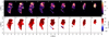 |
Fig. 7. Best-fit results of BCM inversions of the time series presented in Fig. 2. Top row: optical depth; Bottom row: vlos. |
4.1. Optical depth
The optical depth maps in the top row of Fig. 7 show that the overall structure of the fan is reasonably uniform. The inversions for most of the pixels give a τ0 value close to 8 (purple), with some higher opacity regions where the τ0 can reach around 20. In regions where the cloud model assumptions break down, sometimes anomalous values of τ0 greater than 100 are returned. This is mainly due to the fact that the variations in the profile background become large compared to the slope of the wing or shape of the core. This made the code prioritize fitting variations in broadened flare background profiles over the overall shape of the absorption profile. Greater values are typically found at the top of the fan and were removed by the mask. The very top of the fan is a region in which some of the BCM modeling assumptions become less accurate, for example when it is not true that the fan is backlit in the LOS by the same spectrally broad flare ribbon emission (see Figs. 2, 1–3).
The model also breaks down in cases where the optical depth is too low for the core of the line profiles to saturate and thus flatten (e.g., the blue line in Fig. 1f). This case leads to an overestimation of the source function, which results in a higher fitted optical depth (Díaz Baso et al. 2018). In other works this problem was typically solved by taking  (e.g., Paletou 1997; Heinzel & Anzer 2006; Labrosse et al. 2010) to avoid the degeneracy between τ0 and S (Díaz Baso et al. 2018). However, in our case we know S for pixels where the fan material gives a saturated line profile, and this degeneracy arises only for a small number of pixels where the fan material is optically thin.
For this reason we capped the value for τ0 at 30. This preserves all the reliable results derived from inversions of pixels within the main body of the fan, while avoiding anomalous and unreliable results from a few pixels dominating the mass estimate. Later in the time sequence this issue becomes more pronounced due to the heating of material in the fan, which results in a dramatic increase in the number of inversions with low saturation that had much larger uncertainties. Because these problems became increasingly acute with time, we restricted our analysis to the subset of the time sequence for which the results were reliable.
4.2. Velocity of the collapse
The derived LOS velocity, shown in the lower row of Fig. 7, displays higher values at the base of the fan jet and for a greater fraction of the mask as time progresses, in line with the expected behavior as the fan collapses. It also shows generally higher values in LOS velocity and τ toward the top of the FoV, strongly suggesting that the inclination of the fan to the observer is greater in these locations, this is corroborated further by the fact that LOS velocities shrink toward zero or are slightly oriented toward the observer (blueshifted) at the very bottom of the FoV in the mask.
The POS collapse of the fan was tracked (see Sect. 3.3) along six spines that are illustrated in Fig. 6a. The fitted acceleration in this plane was found to be aPOS = 0.29 ± 0.19 km s−2. When combined with the values found in the LOS, we obtain an acceleration of aabs = 0.39 ± 0.12 km s−2. This is within the error bars for acceleration under solar gravity and other forces not playing a significant role, which is also consistent with the findings of Morton (2012) and Robustini et al. (2016), but not with those of Roy (1973c) and Reid et al. (2018) where a decelerating force is reported. A possible explanation for the absence of this deceleration is that the processes that cause the upward jets of the fan are suppressed by the flare ribbon and that there is no upward-moving fan material in the same plane as the downward-moving fan material. As mentioned earlier, a small signature of the base of the fan remained after the main collapse, which could alternatively be interpreted as a deceleration of the original collapse near the base. This can be seen in the blue line of observed mass in Fig. 8a at times after 60 s.
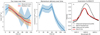 |
Fig. 8. Results of the cloud and slab modeling for the collapse of the fan-shaped jet. a: observed total mass of jet over time (blue). Simulated fan collapse based on second time frame assuming acceleration under gravity (red). b: delivered momentum to solar surface over time. c: Ca II 8542 Å STiC inversion of flare background (gray dashed), obtained from observed profile (gray). Ca II 8542 Å fan profile (black) fitted from background profile with an absorbing slab above it. |
However, the uncertainties in these results are quite large, and increase dramatically after frame 5, due to issues such as ionization of the plasma, and so we are not able to complete a full study of the collapse using solely the observational data. Therefore, in our model of the complete collapse of the fan we use the mass distribution that was derived observationally from the first frames, and assume that the structure collapsed under gravity, as was suggested by the frames that are most reliable for the estimation of the acceleration in the collapse. The maximum absolute velocity of falling material at the bottom of the fan is 70 km s−1.
4.3. Fan mass
Using the relations shown in Sect. 3.1 we can convert our reported optical depth values into masses, and subsequently use an estimate of the geometrical thickness of the fan to convert the masses into densities. The total mass for each of the nine time frames shown in Fig. 2 is plotted in blue in Fig. 8a, with the peak value of 3.9 ± 0.7 × 10¹³ g being found in the second time frame at the start of the collapse. This is significantly smaller than the value of 1015 g suggested by Roy (1973c) for a large surge, based on the assumption of an isotropic expansion of an initial density of 3 × 10¹⁵ particles cm−3 from the base of the surge. This discrepancy could be due to the simpler assumptions used in Roy’s estimate, to the smaller size of our surge, or to a natural variation in the physical parameters of such jets. However, the height of the fan observed in Roy’s work was 10 times greater than that reported here. Multiplying the mass estimate of our fan by a factor of 10 to account for this height difference produces mass estimates that are only separated by a factor of 3.
The similar masses in the first and second frames, and the nearly identical shapes of the fan in these two frames (see Fig. 2), suggests that the collapse does not start until the second time frame. From the second to the fifth frames we get a smooth collapse, after which the observed total mass starts to fluctuate. This is also the time frame when the ionization of the fan begins to dominate the opacity changes in significant fractions of the total area of the fan jet. However, we note that the collapse seems to halt as the fan persists for a number of frames at a much smaller size of around 2 Mm.
The total masses derived from the collapse described in Sect. 3.3 is overplotted in red in Fig. 8a, with error estimates shown using the lighter shading. This collapse was modeled using the mass distribution from the second frame and gravitational acceleration, starting at the second time frame. We can see that it matches the observed collapse (blue curve) very well for the first three time steps (15−60 s), after which the values derived from the two methods diverge and large error estimates affect the observational values. From this data it seems that there is still a smaller vertical range near the base over which the fan-shaped jet was acting and interacting with the flare ribbon during this time, but that the material higher up continued collapsing under gravity. Thus, the picture is less clear after 60 s in the data.
4.4. Fan density
Using the above-mentioned assumption that the fan has a uniform thickness of 200 km (based on the width of the thinnest resolved structures in the POS direction), we also report estimated mean densities. For the convenience of the reader we provide this number in three different unit formats, 2 ± 0.3 × 10⁻⁸ kg m−3, 2 ± 0.3 × 10⁻¹¹ g cm−3, and 9 ± 1.4 × 10¹² particles cm−3. This is a typical value for chromospheric material and within the same order of magnitude as the value of 1012 particles cm−3 suggested by Roy (1973c) for a large surge, based on the assumption of an isotropic expansion of an initial density of 3 × 10¹⁵ particles cm−3 from the base of the surge. Our value is also consistent with values for the simulated chromospheric jets reported by Takasao et al. (2013). Kayshap et al. (2013) reported a much lower value of 4.1 × 10⁹ particles cm−3, but this is for a much hotter surge of 2 MK. We can also compare our densities to similar chromospheric structures; for example, a Bifrost fibril has a typical density of around 10−9 to 10−10 kg m−3 (Druett et al. 2021b), and spicule densities of around 2.2 × 10¹⁰ particles cm−3 have been reported (Sterling 2000; Shimojo et al. 2020).
4.5. Fan temperature
Our second slab model used the STiC code, and allowed us to fit a fan profile7 from the Ca II 8542 Å observations. This was achieved by using a profile from the nearby flare background and a slab with the thickness and density that were reported above, as discussed in Sect. 3.2. In Fig. 8c we can see a Ca II 8542 Å flare background profile in gray and a fan profile in black. The dashed gray curve represents the STiC inversion made of the profile, which was then used as the input model for our fan fitting routine. The red curve was obtained from this input model only after modifying the temperature, LOS velocity, and microturbulence of the cloud part of the model. The best-fit temperature for the background was between 10 and 11 kK at chromospheric heights, which matches findings from Yadav et al. (2021). For the slab material the best-fit temperature was around 7050 ± 250 K. The model also produced estimates for the slab material of LOS velocity (4.5 km s−1) and microturbulent velocity (6 km s−1). The LOS velocity is comparable to the value found from the BCM for this pixel of 5.5 ± 1.4 km s−1, which increases our confidence in the temperature estimate, which is typical for chromospheric material, as was required by our assumptions for the relation between τ0 and column mass from Leenaarts et al. (2012).
Robustini et al. (2016) reported an average brightness temperature (i.e., the temperature of a blackbody) that would produce this intensity in the wavelength of the Hα line core of 5.5 kK that was consistent over several different pixels for a similar jet observed in Hα. This is lower than our NLTE inversion value, but matches the Hα brightness temperature calculated using the same pixel that was employed for our inversions by looking at the Hα line core intensity, as described in Robustini et al. (2016). Although these results are consistent, we note that both structures are NLTE and so we should not assume that this brightness temperature value is the true temperature of the plasma, or conclude that the NLTE plasma temperatures of the fan discussed here and the one reported in Robustini et al. (2016) match. Our inverted temperature is lower than the simulated surge temperatures of 105 K or higher, as reported by Nishizuka et al. (2008) and Kayshap et al. (2013); however, these temperatures have been contested by Nóbrega-Siverio et al. (2016) who suggest a typical value around 104 K when radiative losses are considered.
We note that the Hα profile widths of the fan jet material in this dataset are much larger than those reported in Molnar et al. (2019). Extrapolating the best-fit line from this work would suggest temperatures of up to 25 kK for the Hα profiles presented in our work. This is far beyond the ionization temperature of Hα. The majority of broadening in the work of Molnar et al. (2019) was attributed to opacity effects that happened to correlate with changes in the Atacama Large Millimeter/submillimeter Array (ALMA) brightness temperature. The relationship between the line width and plasma temperatures inferred in Molnar et al. (2019) appears to break down in the context presented here.
4.6. Fan momentum and energy
It is possible to deduce an estimate of the momentum delivered at the base of the jet as a function of time by using the model of the collapse of the fan as described in Sect. 3.4. The results of this estimate are shown in Fig. 8b. Most notable here is the nearly constant values between the second and fifth time frame, which peaks at 3.8 ± 0.5 × 10¹⁸ g cm s−1 for a one-second interval. This is at least two orders of magnitude smaller than most of the reported sunquakes (Stefan & Kosovichev 2020), including those found in our dataset. However, as discussed before, it is hard to make a comparison with this number without knowing the time over which the momentum was delivered. If we multiply the number by 40 s, to make the times comparable to the sunquake reported in Zharkova et al. (2020), we end up a factor of 40 below the lowest total momentum of 5.4 × 10²¹ g cm s−1 that was fitted to a sunquake in our dataset by Stefan & Kosovichev (2020). This suggests that our fan jet does not supply sufficient energy to act as the source of a sunquake beneath it. However, if we artificially scale up our fan model to 200 Mm by extending the mass distribution linearly in height, we obtain values with a similar order of magnitude, which opens up the possibility that a large fan jet is an energetically plausible source for triggering a sunquake.
A similar calculation provides an estimate of the energy density flux instead of the momentum. This gives us a value of 1.0 × 10⁹ erg s−1 cm−2, which is three orders of magnitude lower than the lower estimate of 1.5 × 10¹² erg s−1 cm−2 reported by Sharykin et al. (2017). Sharykin et al. (2017) reports on a sunquake that has a total momentum only one order of magnitude higher than the smallest momentum detected for a sunquake to date (Stefan & Kosovichev 2020). In terms of energy density flux we can only reach 10% of the reported value by scaling up the fan to 200 Mm. This suggests that while a similar total momentum flux could be achieved in a larger fan, the area over which the energy is spread might be too large to trigger a visible sunquake.
5. Conclusions
We investigated a small fan jet above a light bridge of a sunspot in AR 12673. The upward jet was suppressed by a flare ribbon that expanded over its base during an X9.3 flare. This ribbon covered the sunspot umbra and prevented the subsequent ejection of material from above the light bridge. This created a unique situation where the remaining material of the fan could be studied while it was falling. Our main focus was on the Hα observations of this dataset, aided by the fact that the flare ribbon profiles had flattened profiles with similar intensities along the entire CRISP wavelength window. This allowed us to employ a simple cloud model to perform inversions that could fit the profiles and deduce estimates of the optical depth of the material in the collapsing jet.
This simple model produced good quality fits to the profiles for most of the pixels in the fan over the course of nine time frames (see Fig. 7), and thus provides estimates of the optical depths and LOS velocities of the material in the fan for each pixel. These optical depths could then be used to estimate the masses of material in each pixel of the fan using the relation from Leenaarts et al. (2012). The peak value for the total mass in the jet came in the second time frame, with a value of 3.9 ± 0.7 × 10¹³ g and a density of 2 ± 0.3 × 10⁻¹¹ g cm−3.
Absolute velocity estimates could be found by combining the LOS velocities in each pixel with the POS velocities obtained from tracking the top edge the fan during the first five time frames of the collapse. The resulting estimates of the acceleration were consistent with solar gravity.
A temperature of 7050 ± 250 K was found for a sample of material in the fan using a second, independent cloud model based on the synthesis mode of the STiC code and an external inversion tool. Here we fitted a Ca II 8542 Å fan profile by first inverting a flare ribbon profile, and using this atmosphere as a background atmosphere for the fitting of the fan profile with an additional slab placed at the upper boundary of the background atmosphere. The fitting routine then estimated the fan profile by only modifying the parameters of the slab (see Fig. 8c). This temperature is lower than that found in literature for similar structures. However, the 5500 K brightness temperature of material in our fan jet matches the value found in Robustini et al. (2016). Our temperature is chromospheric, as was required by our assumptions for the relation between τ0 and column mass from Leenaarts et al. (2012).
In order to achieve an estimate of the momentum delivered to the base of the fan jet, we first constructed a model of the fan collapse. We chose this because effects such as ionization made some parts of the fan transparent during the later stages of its collapse. This made estimates of the acceleration derived from observations unreliable in the later time frames. Moreover, some small jet material remained visible at the base for a while longer. The red curve in Fig. 8a shows values based on the collapse of the initial mass distribution of the fan under gravity, without these effects. From this model of the collapse it was possible to make an estimate of the momentum delivery to the base of the fan against time, which is shown in Fig. 8b. The peak value of this momentum delivery was 3.5 ± 0.5 × 10¹⁹ g cm s−1. This is two orders or magnitude smaller than the momentum delivery reported in most sunquakes (Stefan & Kosovichev 2020), including some found in this dataset (Zharkova et al. 2020) and (Zharkov et al. 2020). However, we note that these momenta are for the entire event, and our value is given as delivery per second. A more meaningful comparison is given by looking at the energy density flux, which gives us a value of 1.0 × 10⁹ erg s−1 cm−2, which is three orders of magnitude lower than the value reported by Sharykin et al. (2017) for a larger sunquake. Therefore, the collapse of this small fan jet can be ruled out as the source of a sunquake in this observation. However, since this is a very small jet, this result does not completely exclude other larger jets from being energetically plausible triggers for sunquakes. Our estimates do suggest, however, that very large jets of 200 Mm or more would be needed to reach values comparable to those that have been observed to date.
Our results were fundamentally enabled by the unique nature of this dataset as we took advantage of a very specific physical setup. Therefore, we cannot easily compare our findings to other datasets with more variable background emission. Thus, a good next step would be to compare our finding to simulated fan-shaped jets. Additionally there are other unique sets of conditions that could yield a similar simplification (such as limb observations). Additionally, one could search for sunquake signatures under larger jets and, if found, attempt to derive estimates of the momentum delivery from falling material in the fan jet in this manner.
Sunquakes were predicted by Wolff (1972) and first observed by Kosovichev & Zharkova (1998).
We used an inversion process similar to the one discussed in Sect. 4.3 of Pietrow et al. (2020).
Which we estimate to be 5.5 Mm × 200 km = 1 × 1016 cm2.
We chose the second frame because it gives the highest mass.
The fitted fan profile was taken at around [x, y] = 5, 7 Mm on Fig. 1, 1.
Acknowledgments
M.D. was supported by The Swedish Research Council, grant number 2017-04099. J.d.l.C.R. gratefully acknowledges funding from the European Research Council (ERC) under the European Union’s Horizon 2020 research and innovation program (SUNMAG, grant agreement 759548). The Swedish 1-m Solar Telescope is operated on the island of La Palma by the Institute for Solar Physics of Stockholm University in the Spanish Observatorio del Roque de los Muchachos of the Instituto de Astrofísica de Canarias. The Institute for Solar Physics was supported by a grant for research infrastructures of national importance from the Swedish Research Council (registration number 2017-00625). Computations were performed on resources provided by the Swedish Infrastructure for Computing (SNIC) at the PDC Centre for High Performance Computing (Beskow, PDC-HPC), at the Royal Institute of Technology in Stockholm as well as the National Supercomputer Centre (Tetralith, NSC) at Linköping University. This work was supported by the Knut and Alice Wallenberg Foundation. This research has made use of NASA’s Astrophysics Data System Bibliographic Services. We acknowledge the community effort devoted to the development of the following open-source packages that were used in this work: numpy (numpy.org), matplotlib (matplotlib.org), astropy (astropy.org). We thank Adur Pastor Yabar and Carlos Diaz Baso for their valuable conversations and suggestions. We thank Mihalis Mathioudakis, Sean Quinn, and Aaron Reid for providing access to the Queen’s University Belfast observational campaign datasets from the SST. UK access to the Swedish 1-m Solar Telescope was funded by the Science and Technology Facilities Council (STFC) under grant No. ST/P007198/1.
References
- Asai, A., Ishii, T. T., & Kurokawa, H. 2001, ApJ, 555, L65 [NASA ADS] [CrossRef] [Google Scholar]
- Beckers, J. M. 1964, PhD Thesis, Sacramento Peak Observatory, Air Force Cambridge Research Laboratories, USA [Google Scholar]
- Bharti, L., Rimmele, T., Jain, R., Jaaffrey, S. N. A., & Smartt, R. N. 2007, MNRAS, 376, 1291 [Google Scholar]
- Bruzek, A., & Durrant, C. J. 1977, Illustrated Glossary for Solar and Solar Terrestrial Physics (Dordrecht: Reidel) [CrossRef] [Google Scholar]
- Byrd, R. H., Lu, P., Nocedal, J., & Zhu, C. 1995, SIAM J. Sci. Comput., 16, 1190 [Google Scholar]
- Capparelli, V., Zuccarello, F., Romano, P., et al. 2017, ApJ, 850, 36 [NASA ADS] [CrossRef] [Google Scholar]
- Cauzzi, G., Reardon, K., Rutten, R. J., Tritschler, A., & Uitenbroek, H. 2009, A&A, 503, 577 [NASA ADS] [CrossRef] [EDP Sciences] [Google Scholar]
- de la Cruz Rodríguez, J., & Piskunov, N. 2013, ApJ, 764, 33 [Google Scholar]
- de la Cruz Rodríguez, J., Löfdahl, M. G., Sütterlin, P., Hillberg, T., & Rouppe van der Voort, L. 2015, A&A, 573, A40 [NASA ADS] [CrossRef] [EDP Sciences] [Google Scholar]
- de la Cruz Rodríguez, J., Leenaarts, J., & Asensio Ramos, A. 2016, ApJ, 830, L30 [Google Scholar]
- de la Cruz Rodríguez, J., Leenaarts, J., Danilovic, S., & Uitenbroek, H. 2019, A&A, 623, A74 [Google Scholar]
- Díaz Baso, C. J., Martínez González, M. J., Asensio Ramos, A., et al. 2018, PhD Thesis, Universidad de La Laguna, Spain [Google Scholar]
- Díaz Baso, C. J., Martínez González, M. J., Asensio Ramos, A., & de la Cruz Rodríguez, J. 2019, A&A, 623, A178 [NASA ADS] [CrossRef] [EDP Sciences] [Google Scholar]
- Diaz Baso, C., Vissers, G., Calvo, F., et al. 2021, https://doi.org/10.5281/zenodo.5608441 [Google Scholar]
- Ding, J. Y., Madjarska, M. S., Doyle, J. G., & Lu, Q. M. 2010, A&A, 510, A111 [NASA ADS] [CrossRef] [EDP Sciences] [Google Scholar]
- Druett, M. K., & Zharkova, V. V. 2018, A&A, 610, A68 [NASA ADS] [CrossRef] [EDP Sciences] [Google Scholar]
- Druett, M., Scullion, E., Zharkova, V., et al. 2017, Nat. Commun., 8, 15905 [NASA ADS] [CrossRef] [Google Scholar]
- Druett, M. K., Pietrow, A. G. M., Vissers, G. J. M., & Robustini, C. 2021a, ArXiv e-prints [arXiv:2111.10786] [Google Scholar]
- Druett, M. K., Leenaarts, J., Carlsson, M., & Szydlarski, M. 2021b, A&A, submitted [arXiv:2112.08245] [Google Scholar]
- Ellison, M. A. 1949, MNRAS, 109, 3 [NASA ADS] [CrossRef] [Google Scholar]
- Harvey, J. W. 1969, PhD Thesis, National Solar Observatory, USA [Google Scholar]
- Heinzel, P., & Anzer, U. 2006, ApJ, 643, L65 [NASA ADS] [CrossRef] [Google Scholar]
- Ichimoto, K., & Kurokawa, H. 1984, Sol. Phys., 93, 105 [NASA ADS] [Google Scholar]
- Joye, W. A., & Mandel, E. 2003, in Astronomical Data Analysis Software and Systems XII, eds. H. E. Payne, R. I. Jedrzejewski, & R. N. Hook, ASP Conf. Ser., 295, 489 [NASA ADS] [Google Scholar]
- Kayshap, P., Srivastava, A. K., & Murawski, K. 2013, ApJ, 763, 24 [NASA ADS] [CrossRef] [Google Scholar]
- Kayshap, P., Singh Payal, R., Tripathi, S. C., & Padhy, H. 2021, MNRAS, 505, 5311 [NASA ADS] [CrossRef] [Google Scholar]
- Kianfar, S., Leenaarts, J., Danilovic, S., de la Cruz Rodríguez, J., & José Díaz Baso, C. 2020, A&A, 637, A1 [NASA ADS] [CrossRef] [EDP Sciences] [Google Scholar]
- Kosovichev, A. G., & Zharkova, V. V. 1998, Nature, 393, 317 [Google Scholar]
- Kuridze, D., Mathioudakis, M., Simões, P. J. A., et al. 2015, ApJ, 813, 125 [Google Scholar]
- Labrosse, N., Heinzel, P., Vial, J. C., et al. 2010, Space Sci. Rev., 151, 243 [Google Scholar]
- Leenaarts, J., Carlsson, M., & Rouppe van der Voort, L. 2012, ApJ, 749, 136 [NASA ADS] [CrossRef] [Google Scholar]
- Levenberg, K. 1944, Q. Appl. Math., 2, 164 [Google Scholar]
- Löfdahl, M. G. 2002, in Society of Photo-Optical Instrumentation Engineers (SPIE) Conference Series, eds. P. J. Bones, M. A. Fiddy, & R. P. Millane, Proc. SPIE, 4792, 146 [Google Scholar]
- Löfdahl, M. G., Hillberg, T., de la Cruz Rodríguez, J., et al. 2021, A&A, 653, A68 [Google Scholar]
- Louis, R. E., & Thalmann, J. K. 2021, ApJ, 907, L4 [NASA ADS] [CrossRef] [Google Scholar]
- Louis, R. E., Beck, C., & Ichimoto, K. 2014, A&A, 567, A96 [NASA ADS] [CrossRef] [EDP Sciences] [Google Scholar]
- Madjarska, M. S., Doyle, J. G., & de Pontieu, B. 2009, ApJ, 701, 253 [CrossRef] [Google Scholar]
- Malville, J. M., & Moreton, G. E. 1961, Nature, 190, 995 [CrossRef] [Google Scholar]
- Marquardt, D. W. 1963, J. Soc. Ind. Appl. Math., 11, 431 [Google Scholar]
- McMath, R. R., & Pettit, E. 1937, ApJ, 85, 279 [NASA ADS] [CrossRef] [Google Scholar]
- Molnar, M. E., Reardon, K. P., Chai, Y., et al. 2019, ApJ, 881, 99 [Google Scholar]
- Morton, R. J. 2012, A&A, 543, A6 [NASA ADS] [CrossRef] [EDP Sciences] [Google Scholar]
- Neckel, H., & Labs, D. 1984, Sol. Phys., 90, 205 [Google Scholar]
- Newton, H. W. 1942, MNRAS, 102, 2 [CrossRef] [Google Scholar]
- Newville, M., Stensitzki, T., Allen, D. B., & Ingargiola, A. 2014, https://doi.org/10.5281/zenodo.11813 [Google Scholar]
- Nishizuka, N., Shimizu, M., Nakamura, T., et al. 2008, ApJ, 683, L83 [NASA ADS] [CrossRef] [Google Scholar]
- Nóbrega-Siverio, D., Moreno-Insertis, F., & Martínez-Sykora, J. 2016, ApJ, 822, 18 [Google Scholar]
- Nóbrega Siverio, D., Guglielmino, S. L., & Sainz Dalda, A. 2021, A&A, 655, A28 [CrossRef] [EDP Sciences] [Google Scholar]
- Paletou, F. 1997, A&A, 317, 244 [NASA ADS] [Google Scholar]
- Pietrow, A. G. M. 2019, https://doi.org/10.5281/zenodo.3229961 [Google Scholar]
- Pietrow, A. G. M., Kiselman, D., de la Cruz Rodríguez, J., et al. 2020, A&A, 644, A43 [NASA ADS] [CrossRef] [EDP Sciences] [Google Scholar]
- Piskunov, N., & Valenti, J. A. 2017, A&A, 597, A16 [NASA ADS] [CrossRef] [EDP Sciences] [Google Scholar]
- Quinn, S., Reid, A., Mathioudakis, M., et al. 2019, ApJ, 881, 82 [NASA ADS] [CrossRef] [Google Scholar]
- Reid, A., Henriques, V. M. J., Mathioudakis, M., & Samanta, T. 2018, ApJ, 855, L19 [NASA ADS] [CrossRef] [Google Scholar]
- Robustini, C., Leenaarts, J., de la Cruz Rodriguez, J., & Rouppe van der Voort, L. 2016, A&A, 590, A57 [NASA ADS] [CrossRef] [EDP Sciences] [Google Scholar]
- Robustini, C., Leenaarts, J., & de la Cruz Rodríguez, J. 2018, A&A, 609, A14 [NASA ADS] [CrossRef] [EDP Sciences] [Google Scholar]
- Roy, J. R. 1973a, PhD Thesis, The University of Western Ontario, Canada [Google Scholar]
- Roy, J. R. 1973b, Sol. Phys., 28, 95 [NASA ADS] [CrossRef] [Google Scholar]
- Roy, J. R. 1973c, Sol. Phys., 32, 139 [NASA ADS] [CrossRef] [Google Scholar]
- Scharmer, G. 2017, SOLARNET IV: The Physics of the Sun from the Interior to the Outer Atmosphere, 85 [Google Scholar]
- Scharmer, G. B., Bjelksjo, K., Korhonen, T. K., Lindberg, B., & Petterson, B. 2003, in Innovative Telescopes and Instrumentation for Solar Astrophysics, eds. S. L. Keil, & S. V. Avakyan, SPIE Conf. Ser., 4853, 341 [NASA ADS] [CrossRef] [Google Scholar]
- Scharmer, G. B., Narayan, G., Hillberg, T., et al. 2008, ApJ, 689, L69 [Google Scholar]
- Schmieder, B., Golub, L., & Antiochos, S. K. 1994, ApJ, 425, 326 [NASA ADS] [CrossRef] [Google Scholar]
- Sharykin, I. N., & Kosovichev, A. G. 2020, ApJ, 895, 76 [NASA ADS] [CrossRef] [Google Scholar]
- Sharykin, I. N., Kosovichev, A. G., Sadykov, V. M., Zimovets, I. V., & Myshyakov, I. I. 2017, ApJ, 843, 67 [NASA ADS] [CrossRef] [Google Scholar]
- Shimizu, T. 2009, in The Second Hinode Science Meeting: Beyond Discovery-Toward Understanding, eds. B. Lites, M. Cheung, T. Magara, J. Mariska, & K. Reeves, ASP Conf. Ser., 415, 148 [Google Scholar]
- Shimizu, T., Katsukawa, Y., Kubo, M., et al. 2009, ApJ, 696, L66 [Google Scholar]
- Shimojo, M., Kawate, T., Okamoto, T. J., et al. 2020, ApJ, 888, L28 [Google Scholar]
- Stefan, J. T., & Kosovichev, A. G. 2020, ApJ, 895, 65 [NASA ADS] [CrossRef] [Google Scholar]
- Sterling, A. C. 2000, Sol. Phys., 196, 79 [NASA ADS] [CrossRef] [Google Scholar]
- Sterling, A. C., Shibata, K., & Mariska, J. T. 1993, ApJ, 407, 778 [NASA ADS] [CrossRef] [Google Scholar]
- Takasao, S., Isobe, H., & Shibata, K. 2013, PASJ, 65, 62 [Google Scholar]
- Tsiropoula, G. 1999, in Magnetic Fields and Solar Processes, ed. A. Wilson, ESA Spec. Publ., 9, 395 [NASA ADS] [Google Scholar]
- Tziotziou, K. 2007, in The Physics of Chromospheric Plasmas, eds. P. Heinzel, I. Dorotovič, & R. J. Rutten, ASP Conf. Ser., 368, 217 [NASA ADS] [Google Scholar]
- Tziotziou, K., Heinzel, P., & Tsiropoula, G. 2007, A&A, 472, 287 [NASA ADS] [CrossRef] [EDP Sciences] [Google Scholar]
- Uddin, W., Schmieder, B., Chandra, R., et al. 2012, ApJ, 752, 70 [NASA ADS] [CrossRef] [Google Scholar]
- Uitenbroek, H. 2001, ApJ, 557, 389 [Google Scholar]
- van Noort, M., Rouppe van der Voort, L., & Löfdahl, M. G. 2005, Sol. Phys., 228, 191 [Google Scholar]
- Vissers, G., & Rouppe van der Voort, L. 2012, ApJ, 750, 22 [Google Scholar]
- Vissers, G. J. M., Danilovic, S., de la Cruz Rodríguez, J., et al. 2021, A&A, 645, A1 [NASA ADS] [CrossRef] [EDP Sciences] [Google Scholar]
- Wolff, C. L. 1972, ApJ, 176, 833 [NASA ADS] [CrossRef] [Google Scholar]
- Wuelser, J.-P., & Marti, H. 1989, ApJ, 341, 1088 [NASA ADS] [CrossRef] [Google Scholar]
- Yadav, R., Díaz Baso, C. J., de la Cruz Rodríguez, J., Calvo, F., & Morosin, R. 2021, A&A, 649, A106 [NASA ADS] [CrossRef] [EDP Sciences] [Google Scholar]
- Yokoyama, T., & Shibata, K. 1995, Nature, 375, 42 [Google Scholar]
- Yoshimura, K., Kurokawa, H., Shimojo, M., & Shine, R. 2003, PASJ, 55, 313 [CrossRef] [Google Scholar]
- Zarro, D. M., Canfield, R. C., Strong, K. T., & Metcalf, T. R. 1988, ApJ, 324, 582 [NASA ADS] [CrossRef] [Google Scholar]
- Zharkov, S., Matthews, S., Zharkova, V., et al. 2020, A&A, 639, A78 [EDP Sciences] [Google Scholar]
- Zharkova, V., Zharkov, S., Druett, M., Matthews, S., & Inoue, S. 2020, A&A, 639, A79 [NASA ADS] [CrossRef] [EDP Sciences] [Google Scholar]
- Zhou, Y. H., Chen, P. F., Hong, J., & Fang, C. 2020, Nat. Astron., 4, 994 [NASA ADS] [CrossRef] [Google Scholar]
All Figures
|
Fig. 1. Overview of AR 12673 taken on 6 September 2017 at 11:59 UT. The fan jet is indicated by a white rectangle. Panel a: continuum intensity 4000 Å; b: Ca II 8542 Å line core intensity; c: Ca II K line core intensity; d: Hα line core intensity; e: enlarged view of white rectangle in panel d. The red, blue, green, and orange dots show the physical locations from which the profiles shown in panel f were taken; f: Hα profiles of flare ribbon (red) and fan jet (blue, green, yellow). |
| In the text | |
|
Fig. 2. Time series of fan jet from 11:59 UT to 12:01 UT with 15 s between each panel. |
| In the text | |
|
Fig. 3. Cartoon showing a simplified side-on view of the physical situation being studied at two optical depth values for the photosphere and chromosphere. A fan jet is situated above a light bridge with a hot flare ribbon behind it. From our perspective the fan is backlit by the ribbon. |
| In the text | |
|
Fig. 4. Plot of examples of Hα profiles from pixels containing the fan jet (black) and the fit using the BCM including (red) and excluding (blue) the two outermost wavelength points. Top: fitted profile with a low χ2, showing good agreement between the blue and red curves. Bottom: profile with asymmetrical far wings that caused a high χ2 value in the original fit, and a much better fit to the main component shown by the blue curve. |
| In the text | |
|
Fig. 5. Stratification in geometrical height scale of parameters (T, vlos, vturb) inverted with our second cloud model (described in Sect. 3.2) as well as the inferred density from the first cloud model (described in Sect. 3.1). The black line shows the stratification of these parameters for the flare ribbon background, while the red line compares these same parameters for the best fit of an inverted pixel inside of the fan. Note that the model stratification is fixed everywhere except in the slab at the top of the atmosphere. Panel a: temperature; panel b: LOS velocity; panel c: microtubulence; and panel d: density. The observed and best-fit profiles belonging to these atmospheres can be found in Fig. 8c. |
| In the text | |
|
Fig. 6. Collapse of the fan tracked along six spines. Panel a: minimum value of the Hα emission intensity. This shows the fan in the first time frame (11:59:20 UT). The six spines used are shown using black lines, with a white dot denoting the edge of the fan as derived from the process shown in panel b. Panel b: LOS velocity values on the y-axis (normalized to the same maximum value for comparison) against position along the length of the spine in pixels on the x-axis (zero being the base of the spine). This data is shown at six different times (in different colors) for the fourth spine from the top. |
| In the text | |
|
Fig. 7. Best-fit results of BCM inversions of the time series presented in Fig. 2. Top row: optical depth; Bottom row: vlos. |
| In the text | |
|
Fig. 8. Results of the cloud and slab modeling for the collapse of the fan-shaped jet. a: observed total mass of jet over time (blue). Simulated fan collapse based on second time frame assuming acceleration under gravity (red). b: delivered momentum to solar surface over time. c: Ca II 8542 Å STiC inversion of flare background (gray dashed), obtained from observed profile (gray). Ca II 8542 Å fan profile (black) fitted from background profile with an absorbing slab above it. |
| In the text | |
Current usage metrics show cumulative count of Article Views (full-text article views including HTML views, PDF and ePub downloads, according to the available data) and Abstracts Views on Vision4Press platform.
Data correspond to usage on the plateform after 2015. The current usage metrics is available 48-96 hours after online publication and is updated daily on week days.
Initial download of the metrics may take a while.