| Issue |
A&A
Volume 659, March 2022
|
|
|---|---|---|
| Article Number | A134 | |
| Number of page(s) | 25 | |
| Section | Interstellar and circumstellar matter | |
| DOI | https://doi.org/10.1051/0004-6361/202142339 | |
| Published online | 05 April 2022 | |
Chemistry of nebulae around binary post-AGB stars: A molecular survey of mm-wave lines*,**
1
Observatorio Astronómico Nacional (OAN-IGN),
Alfonso XII 3,
28014
Madrid,
Spain
e-mail: This email address is being protected from spambots. You need JavaScript enabled to view it.
2
Observatorio Astronómico Nacional (OAN-IGN),
Apartado 112,
28803
Alcalá de Henares,
Madrid,
Spain
3
Centro de Desarrollos Tecnológicos, Observatorio de Yebes (IGN),
19141
Yebes,
Guadalajara,
Spain
Received:
30
September
2021
Accepted:
21
January
2022
Abstract
Context. There is a class of binary post-asymptotic giant branch (post-AGB) stars that exhibit remarkable near-infrared excess. Such stars are surrounded by Keplerian or quasi-Keplerian disks, as well as extended outflows composed of gas escaping from the disk. This class can be subdivided into disk- and outflow-dominated sources, depending on whether it is the disk or the outflow that represents most of the nebular mass, respectively. The chemistry of this type of source has been practically unknown thus far.
Aims. Our objective is to study the molecular content of nebulae around binary post-AGB stars that show disks with Keplerian dynamics, including molecular line intensities, chemistry, and abundances.
Methods. We focused our observations on the 1.3, 2, 3 mm bands of the 30mIRAM telescope and on the 7 and 13 mm bands of the 40 m Yebes telescope. Our observations add up ~600 h of telescope time. We investigated the integrated intensities of pairs of molecular transitions for CO, other molecular species, and IRAS fluxes at 12, 25, and 60 μm. Additionally, we studied isotopic ratios, in particular 17O/18O, to analyze the initial stellar mass, as well as 12CO/13CO, to study the line and abundance ratios.
Results. We present the first single-dish molecular survey of mm-wave lines in nebulae around binary post-AGB stars. We conclude that the molecular content is relatively low in nebulae around binary post-AGB stars, as their molecular lines and abundances are especially weaker compared with AGB stars. This fact is very significant in those sources where the Keplerian disk is the dominant component of the nebula. The study of their chemistry allows us to classify nebulae around AC Her, the Red Rectangle, AI CMi, R Sct, and IRAS 20056+1834 as O-rich, while that of 89 Her is probably C-rich. The calculated abundances of the detected species other than CO are particularly low compared with AGB stars. The initial stellar mass derived from the 17O/18O ratio for the Red Rectangle and 89 Her is compatible with the central total stellar mass derived from previous mm-wave interferometric maps. The very low 12CO/13CO ratios found in binary post-AGB stars reveal a high 13CO abundance compared to AGB and other post-AGB stars.
Key words: stars: AGB and post-AGB / binaries: general / circumstellar matter / radio lines: stars / planetary nebulae: general
Spectra are only available at the CDS via anonymous ftp to cdsarc.u-strasbg.fr (130.79.128.5) or via http://cdsarc.u-strasbg.fr/viz-bin/cat/J/A+A/659/A134
Based on observations with the 30 m IRAM and the 40 m Yebes telescopes. IRAM is supported by INSU/CNRS (France), MPG (Germany), and IGN (Spain).
© ESO 2022
1 Introduction
The spectacular late evolution of low- and intermediate-mass stars (main sequence masses in the approximate range of 0.8-8 M⊙) is characterized by a very copious loss of mass during the asymptotic giant branch (AGB) phase. These kinds of stars experience mass loss rates up to 10−4 M⊙ a−1 that dominate the evolution in this phase1. The ejected material creates an expanding circumstellar envelope (CSE). These stars are considered one of the most relevant contributors of dust and enriched material to the Interstellar Medium (ISM); see Gehrz (1989); Matsuura et al. (2009). This environment is favorable for the formation of simple molecules and dust. We find three different kinds of envelopes depending on the C/O ratio: the M-type stars with C/O < 1, the S-type stars with C/O ≈ 1, and C-type with C/O > 1. The kind of molecules and dust grains found in CSEs is determined by the C/O ratio. We find O-bearing molecules, such as SiO or H2O, and silicate dust in M-type stars, making the envelope of these stars O-rich (Engels 1979; Velilla Prieto et al. 2017). On the contrary, we find C-bearing molecules, such as HCN and CS, often alongside SiS, in C-type stars (Olofsson et al. 1993; Cernicharo et al. 2000). Amorphous carbon dust formed out of primary carbon is dominant in C-rich envelopes, while silicon carbide and magnesium sulphide are minor widespread dust components (Zhukovska & Gail 2008; Massalkhi et al. 2020).
Molecular lines were analysed in a large sample of evolved stars (Bujarrabal et al. 1994b,a). The authors investigate line ratios between CO and other O- and C-bearing species to analyze the molecular intensities of these sources. They also study O- and C-bearing molecule ratios to find the necessary criteria to discern between O- and C-rich envelopes around evolved stars. They found, in particular, that SiO and HCN lines can be as intense as CO lines in O- and C-rich stars, respectively.
When the star attains the post-asymptotic giant branch (post-AGB) phase, the expanding envelope becomes a pre-planetary nebula (pPN). The final stage of the evolution of the (low- or intermediate-mass) star is heralded when the exposed core, a white dwarf, ionizes the circumstellar nebula and becomes a planetary nebula (PN). The chemical behaviour in pPNe is more complex than for normal circumstellar envelopes around AGB stars; since O- and C-rich pPNe could present differences in the line ratios compared with O- and C-rich stars (Bujarrabal et al. 1994b). For example, SiO is systematically weaker in pPNe than in evolved stars, while HCN appears to show the opposite trend.
The chemical evolution during the AGB to pPN to PN phases has been investigated in several surveys (Bujarrabal et al. 1994b,a; Bujarrabal 2006; Cernicharo et al. 2011). The star experiences striking changes in the molecular composition at the pPN phase (Pardo et al. 2007; Park et al. 2008; Zhang et al. 2013). However, the chemistry in pPN is poorly studied, even molecular line surveys of PNe are relatively scarce (Zhang 2017).
There is a kind of binary post-AGB stars (binary systems including a post-AGB star) that systematically shows evidence for the presence of disks orbiting the central stars (Van Winckel 2003; de Ruyter et al. 2006; Bujarrabal et al. 2013a; Hillen et al. 2017). All of them present remarkable near-infrared (NIR) excess and the narrow CO line profiles characteristic of rotating disks. The presence of hot dust close to the stellar system is suspected from their spectral energy distribution (SED) and its disk-like shape has been confirmed by interferometric IR data (Hillen et al. 2017; Kluska et al. 2019). The IR spectra of these sources reveal the presence of highly processed grains, which implies that their disks must be stable structures (Jura 2003; Sahai et al. 2011; Gielen et al. 2011a). The low-J rotational lines of CO have been well studied in sources with NIR excess (Bujarrabal et al. 2013a). They show narrow CO lines and relatively wide wings. These line profiles are similar to those in young stars surrounded by a rotating disk made of remnants of interstellar medium and those expected from disk-emission (Bujarrabal et al. 2005; Guilloteau et al. 2013). These results indicate that the CO emission lines of our sources come from Keplerian (or quasi-Keplerian) disks.
Due to the relatively small size of these disks, deep studies of Keplerian disks around post-AGB stars need high angular-and spectral-resolution. To date, there have been only four well-resolved Keplerian disks identified: in the Red Rectangle (Bujarrabal et al. 2013b, 2016), AC Her (Bujarrabal et al. 2015; Gallardo Cava et al. 2021), IWCar (Bujarrabal et al. 2017), and IRAS 08544–4431 (Bujarrabal et al. 2018). These sources are disk-dominated, because the disks contain most of the material of the nebula (~90% of the total mass), while the rest of the mass (~ 10%), corresponds to an extended bipolar outflow surrounding the disk. Very detailed studies (Gallardo Cava et al. 2021) also show strong indications of the presence of Keplerian disks in 89 Her, IRAS 19125+0343, and R Sct. The nebulae around IRAS 19125+0343 and R Sct are dominated by the expanding component, instead of the Keplerian disk, because ~75% of the total mass is located in the outflow. These sources belong to the outflow-dominated subclass. 89 Her is in an intermediate case in between the disk- and the outflow-dominated sources, because ~50% of the material of the nebula is in the Keplerian disk.
There are other binary post-AGB stars that are surrounded by a Keplerian disk that have only been studied with low angular resolution, all of them presenting NIR excess and narrow CO line profiles characteristic of rotating disks (Bujarrabal et al. 2013a).
The chemistry of this class of binary post-AGB sources with Keplerian disks has been practically unknown, with only CO having been very well observed. Furthermore, H13CN, C I, C II were also detected in the Red Rectangle and two maser emission lines were found in AI CMi. In this work, we present a deep and wide survey of radio lines in ten of these sources. All of them have been observed in the 7 and 13 mm bands, and most of them have also been observed at 1.3,2, and 3 mm. The scarce literature about the molecular composition in very evolved objects shows that pPNe display dramatic changes in the chemical composition in the molecular gas with respect to that of their AGB circumstel-lar progenitors. Nevertheless, this kind of nebulae surrounding binary post-AGB stars seem to present a relatively low molecular content. Here we carry out an analysis to explore whether this lower abundance depends on the specific subclass of the binary post-AGB star (disk- or outflow-dominated sources). Additionally, we want to investigate the possibility of classifying some of our objects as O- / C-rich, based on line ratios of different molecules.
This paper is laid out as follows. We present our binary post-AGB star sample in Sect. 2, where relevant results from previous observations are given. Technical information on our observations is presented in Sect. 3 for both telescopes (30mIRAM and 40 m Yebes). We provide our spectra in Sect. 4. Detailed discussions about molecular intensities, chemistry, abundances, and isotopic ratio analysis can be found in Sect. 5. Finally, we summarize our conclusions in Sect. 6.
Binary post-AGB stars observed in this paper.
2 Description of the sources and previous results
We performed single-dish observations of ten sources (Table 1) using the 30mIRAM and the 40mYebes telescopes. These sources are identified as binary post-AGB stars with far-infrared (FIR) excess that is indicative of material ejected by the star. All of them also show significant NIR excess (see Fig. A.1) characteristic of rotating disks (Oomen et al. 2018). They have been poorly studied in the overall search for molecules other than CO. We adopted the distances used in Bujarrabal et al. (2013a). We refrained from measuring distances via parallax measurements, because in the case of binary stars, it is overly complex (Dominik et al. 2003). The velocities are derived from the single-dish and interferometric observations (Bujarrabal et al. 2013a, 2015, 2016, 2017, 2018; Gallardo Cava et al. 2021).
2.1 AC Her
AC Her is a binary post-AGB star (Oomen et al. 2019). Recent mm-wave interferometric observations confirm that AC Her presents a Keplerian disk that clearly dominates the nebula. Observational data and models are compatible with a very diffuse outflowing component surrounding the rotating component. The nebula presents a total mass of 8.3 × 10⁻³ M⊙ and we find that the mass of the outflow must be ≲ 5%. The rotation of the disk is compatible with a central total stellar mass of ~1 M⊙ (Gallardo Cava et al. 2021). The molecular content of this source was unknown, except for the well-studied CO lines (Bujarrabal et al. 2013a; Gallardo Cava et al. 2021).
2.2 Red Rectangle
The Red Rectangle is the best-studied object of our sample. It is a binary post-AGB star (Oomen et al. 2019), with an accretion disk that emits in the UV (Witt et al. 2009; Thomas et al. 2013). This UV emission excite a central H II region (Jura et al. 1997; Bujarrabal et al. 2016) and must also yield a Photo Dissociation Region (or Photon-Dominated Regions, or PDR) between the H II region and the extended Keplerian disk.
Its mm-wave interferometric maps reveal that the nebula contains a rotating disk, containing 90% of the total nebular mass (1.4 × 10⁻² M⊙, see Bujarrabal et al. 2016), together with an expanding low-mass component. The CO line profiles of the Red Rectangle are narrow and present weak wings (Bujarrabal et al. 2013a). Bujarrabal et al. (2016) find high excitation lines: C17O J = 6−5 and H13CN J = 4−3. The C17O line is useful to study regions closer than 60 AU from the central binary star. The presence of the H13CN line means that this molecule is significantly abundant in the central region of the disk, more precisely, closer than 60 AU. The detection of C I, C II, H13CN, and FIR lines is consistent with the presence of a PDR (see e.g. Agúndez et al. 2008), because these lines are the best tracers of these regions.
2.3 89 Her
This source is a binary post-AGB star with NIR excess that implies the presence of hot dust (de Ruyter et al. 2006). The dust is in a stable structure where large dust grains form and settle to the midplane (Hillen et al. 2013, 2014). 89 Her was studied in detail in mm-wave interferometric maps by Gallardo Cava et al. (2021). The nebula contains an extended hourglass-like component and a rotating disk in its innermost region. The total mass of the nebula is 1.4 × 10⁻² M⊙ and the outflow mass represents, at least, 50%.
The molecular content of this source was very poorly studied, except for the single-dish CO observations, which show narrow lines similar to those of the Red Rectangle, but with more prominent wings (Bujarrabal et al. 2013a).
2.4 HD 52961
This source is a binary post-AGB star (Gielen et al. 2011b; Oomen et al. 2018). It presents relatively narrow CO line profiles. Its molecular content was poorly known. Gielen et al. (2011b) found CO2 and the fullerene C60. According to these authors, this source could be O-rich based on its strong similarities to an other post-AGB disk source (EPLyr).
2.5 IRAS 19157–0257 and IRAS 18123+0511
IRAS 19157–0257 and IRAS 18123+0511 are also binary post-AGB stars (Oomen et al. 2019; Scicluna et al. 2020).
The variability of IRAS 19157–0257 is cataloged as irregular (Kiss et al. 2007). Its CO line profiles show relatively narrow lines that are similar to those of 89 Her. The nebular mass is 1.3 × 10⁻² M⊙ (Bujarrabal et al. 2013a). Its molecular content, apart from CO, was unknown.
IRAS 18123+0511 show wide CO line profiles (similar to those found in IRAS 19125+0343). Its nebular mass is 4.7 × 10⁻² M⊙ (Bujarrabal et al. 2013a). No molecular species apart from CO have been detected in these sources despite numerous previous observations (Gómez et al. 1990; Lewis 1997; Deguchi et al. 2012; Liu & Jiang 2017). Our new data improve the rms values of other works.
2.6 IRAS 19125+0343
IRAS 19125+0343 is a binary post-AGB star (Gielen et al. 2008), which also belongs to this class of binary post-AGB star with remarkable NIR excess (Oomen et al. 2019). Recent mm-wave interferometric observations and models reveal that the nebula around this binary post-AGB star is composed of a rotating disk with Keplerian dynamics and an extended outflowing component around it (Gallardo Cava et al. 2021). The total mass of the nebula is 1.1 × 10⁻² M⊙ and the outflow mass represents 70%. The CO lines of this source are narrow but present prominent wings (Bujarrabal et al. 2013a). Apart from CO, the molecular content of this source was unknown.
2.7 AI CMi
AI CMi is an irregular pulsating star with variable amplitude and multiperiodicity that is in an early transition phase from the AGB to the post-AGB stage. The spectral type at maxima is G5 – G8 I (Arkhipova et al. 2017).
According to the analysis of the CO lines, AI CMi presents a nebula (1.9 × 10⁻² M⊙) in which the expanding shell, with a velocity of ~4kms−1, would dominate the whole structure (Bujarrabal et al. 2013a; Arkhipova et al. 2017).
AI CMi shows a detached dust shell with T ~ 200 K and it also presents TiO absorption bands that are formed in the upper cool layers of the extended atmosphere (Arkhipova et al. 2017). This source has been previously observed in radio lines. te Lintel Hekkert et al. (1991) discovered the OH maser at 1612 MHz in a survey of IRAS sources. The H2O maser at 22235.08 MHz was discovered by Engels & Lewis (1996). Suárez etal. (2007); Yoon et al. (2014) studied this source looking for SiO maser emission, but without success. In view of the above results, AI CMi most likely is an O-rich source (see also Arkhipova et al. 2017).
2.8 IRAS 20056+1834
This source has been studied in CO by Bujarrabal et al. (2013a) and the analysis yields a nebular mass of 10−1 M⊙, of which ~22% corresponds to the mass of the disk. Apart from CO, there is no other molecular line detection in this source.
2.9 RSct
The bright RV Tauri variable R Sct shows very irregular pulsations with variable amplitude (Kalaee & Hasanzadeh 2019) and a small IR excess (Kluska et al. 2019), indicating that the SED is not clearly linked to the presence of a circumbinary disk. Nevertheless, the CO integrated flux of the innermost region of the nebula around R Sct shows a characteristic double peak, suggesting the presence of rotation. Models for a disk with Keplerian dynamics and a very extended outflow are consistent with mm-wave interferometric observational data (see Gallardo Cava et al. 2021, for more details). The nebular mass is 3.2 × 10⁻² M⊙, where ~75% corresponds to the mass of the outflow. The hypothesis of a rotating disk is reinforced by interferometric data in the H-band showing a very compact ring (Kluska et al. 2019). The binarity of R Sct is still questioned, but as Keplerian disks are only detected around binaries in the case of evolved stars, it could well be binary as well.
In particular, RSct presents composite CO line profiles including a narrow component, which very likely represents emission from the rotating disk (Bujarrabal et al. 2013a; Gallardo Cava et al. 2021). The chemistry of this source has been studied in IR by Matsuura et al. (2002) and Yamamura et al. (2003), who find that the IR spectra of R Sct is dominated by molecular emission features, especially from H2O. These molecules are probably located in a spherical extended atmosphere. In addition, SiO, CO2, and CO bands have been identified. Lebre & Gillet (1991) detected photospheric absorption Fe I lines, with the double absorption and emission Ti I profiles observed, as well as TiO.
Observed frequency ranges.
3 Observations and data reduction
Our observations were performed using the 30mIRAM telescope (Granada, Spain) and the 40 m Yebes telescope (Guadalajara, Spain). We observed at the 1.3, 2, 3, 7, and 13 mm bands (see Table 2). Our observations required a total telescope time of ~600h distributed over two the telescopes and for several projects (see Table 2).
The data reduction was carried out with the software CLASS2 within the GILDAS3 software package. For each source, we applied the standard procedure of data reduction that consists of rejecting bad scans, averaging the good ones, and subtracting a baseline of a first-order polynomial.
3.1 30 m IRAM telescope
We observed at the 1.3,2, and 3 mm bands using the 30 m IRAM telescope. Our observations were performed in four different projects. Observations of 89 Her, RSct, and the Red Rectangle were obtained between 13 and 19 February 2019 under project 179-18 for 80 h. The data of project 055-19 were obtained between 29 June and 1 July 2019, when we observed the Red Rectangle for an additional 62 h. IRAS 19125+0343 and IRAS 20056+1834 were observed between 9 September and 14 September 2020 for 42 h within project 042-20. As a continuation of the last project, we also observed AI CMi and HD 52961 between 24 and 29 November 2020 for 45 h. Finally, observations of AC Her, IRAS 19157–0257, and IRAS 18123+0511 were obtained between 21 and 27 July 2021, and 27 August 2021 under project E04-20 for 90 h.
We connected the Fast Fourier Transform Spectrometer (FTS) units to the EMIR receiver with a resolution of 200kHz per channel. The Half Power Beam Width (HPBW) of the 30 m IRAM telescope is 11″, 17″, and 28″ at 224, 145, and 86 GHz, respectively. The sources were observed using the wobbler-switching mode, which provides flat baselines. The subreflector was shifted every 2 s with a throw of ±120″ in the azimuth direction. We obtained spectra for the vertical and horizontal linear polarization receivers. Both polarizations were obtained simultaneously and we did not find significant differences in their relative calibration.
The calibration was derived using the chopper-wheel method observing the sky, and hot and cold loads. The procedure was repeated every 15–20 min, depending on the weather conditions. The observed peak emission values have been re-scaled (if applicable) comparing with the intensity of calibration lines observed in NGC7027 and CWLeo (IRC+10216). The absolute scale accuracy is of the order of 10, 10, and 20% in the 3, 2, and 1.3 mm receives, respectively.
3.2 40 m Yebes telescope
We observed at the 7 and 13 mm bands using the 40 m Yebes telescope, Q- and K-band, respectively. We performed our observations in the course of two projects. We observed all the sources of our sample at 7 mm between 29 May and 7 June 2020 for 50 h under project 20A009. In the same project, we also observed at 13 mm between 20 and 27 May 2020 for 15 h. The data of project 20B006 were obtained in several epochs, between 6 and 13 June, 24 and 26 November 2020, and 14 and 17 January 2021. We observed AI CMi, IRAS 20056+1834, the Red Rectangle, 89 Her, AC Her, HD 52961 and IRAS 19125+0343 at 7 mm for 70 h. We also observed IRAS 20056 and HD 52961 at 13 mm for 12 h between 24 and 29 October 2020.
The received signal was detected using the Fast Fourier Transform Spectrometer (FFTS) backend units. The bandwidth of the Q-band is 18 GHz, the spectral resolution is 38 kHz, and the HPBW is 37–49”. In this band, our sources were observed using the position-switching method, always using a separation of around 300″ in the azimuthal direction, obtaining flat baselines. We obtained spectra for the vertical and horizontal linear polarization simultaneously and we do not find significantly differences in their flux density calibration; see Tercero et al. (2021) for further technical details. The bandwidth of the K-band is 100 MHz, the spectral resolution is 6.1kHz, and the HPBW is 79”. Our sources were observed using the position-switching method, using separation of about 600” in the azimuthal direction, obtaining flat baselines. The observations at 13 mm were carried out with dual circular polarization with small calibrations differences of ≤ 20%. Pointing and focus were checked in both Q- and K-bands every hour through pseudo-continuum observations of the SiO v = 1 J = 1–0 and H2O maser emission, respectively, towards evolved stars close to our sources that show intense masers; see de Vicente et al. (2016) for details. The pointing errors were always within 5″–7″.
Detected and tentatively detected lines in this work.
4 Observational results
We compiled a list of the detected molecular transitions, together with upper limits for undetected lines, summarized in Appendix C. Additionally, we summarized the main results from detected and tentatively detected lines in Table 3. The tables list, for the main transitions, the peak intensity flux (I [Jy]), its associated noise (σ [Jy]), the integrated line intensity (∫ I dV[Jy km s–1]), its associated uncertainty (σ (∫ I dV) [Jy km s–1]), the spectral resolution (Sp. Res. [km s–1]), and the velocity centroid of the line measured with respect to the local standard of rest (VLSR [km s–1]).
All our sources were previously detected in CO lines (Bujarrabal et al. 2013a). We present the first detection of other mm-wave lines (see Table 4) in these sources and this work is one of the few that systematically surveyed pPNe in the search for molecules. Our detected lines at 1.3, 2, 3, 7, and 13 mm (Table 3) provide new data for the ten binary post-AGB stars of our survey (Table 1). We detected new lines in the Red Rectangle, 89 Her, AI CMi, IRAS 20056+1834, and R Sct. We also present significant upper limits for a large number of lines (see Appendix C), which often include valuable information.
Molecular transitions detected in this work.
4.1 AC Her
We observed this source at 1.3, 2, 7, and 13 mm, resulting in no positive detections, attaining an rms of 15, 9, 7, and 36mJy, respectively (see Table C.1). We also observed AC Her at 3 mm, where we attained a rms value of 4 mJy, and we tentatively detected the v = 1 J = 2–1 SiO maser (see Fig. 1).
This tentative detection is centered at ~ 0 km s–1, which is shifted respect to the CO line profiles (Gallardo Cava et al. 2021; Bujarrabal et al. 2013a). We assume that the SiO maser emission would have come from the innermost region of the disk, which shows the highest velocity shifts, explaining the observed velocity.
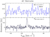 |
Fig. 1 Spectra of the newly tentative maser detection in AC Her. For comparison purposes, we also show the 13CO J = 2–1 line in black (Bujarrabal et al. 2013a). The x-axis indicates velocity with respect to the local standard of rest (VLSR) and the y-axis represents the detected flux measured in Jansky. |
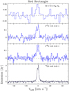 |
Fig. 2 Spectra of the newly detected transitions in the Red Rectangle. For comparison purposes, we also show the 13CO J = 2–1 line in black (Bujarrabal et al. 2013a). The x-axis indicates velocity with respect to the local standard of rest (VLSR) and the y-axis represents the detected flux measured in Jansky. |
4.2 Red Rectangle
The Red Rectangle is the best-studied object of our sample (Bujarrabal et al. 2013a,b, 2016). We present our results in Tables C.2 and 3, and in Figs. 2 and 3 (and A.2). We have detected the rarest CO isotopic species, namely C17O and C18O J = 2–1. The values for the line peak and integrated intensity of the two lines are similar. We have tentatively detected HCN J = 1–0 with signal-to-noise ratio (S/N > 3). This detection is consistent with the presence of H13CN J = 4–3 (Bujarrabal et al. 2016). The presence of these molecules, together with the C I, C II lines, and PAHs, could be due to the development of a PDR in dense disk regions close to the central stellar binary system. The origin of HCN could be photoinduced chemistry, because it has been detected in the innermost regions of several disks in young stars. This fact could be also present in relatively evolved PNe with UV excess (Bublitz et al. 2019), and is predicted by theoretical modelling of the PDR chemistry (e.g., Agúndez et al. 2008).
The line profile of these transitions shows the double peak characteristic of rotating disks (Guilloteau & Dutrey 1998; Bujarrabal et al. 2013a; Guilloteau et al. 2013). It implies that the emission of these molecules comes from the innermost region of the rotating component of the nebula.
In addition, we detected SO JN = 66–54. The line profile of the SO line is narrow, as the CO lines, which suggests that oxygen rich material could be located in the Keplerian disk. We also tentatively detected emission of H2O JKa,Kc = 61,6–52,3. The centroid of this line is 8.3 km s–1, and this shift in velocity could have its origin in maser emission. We have confirmed the detection of H2O maser emission at 325 GHz in our new ALMA maps (priv. comm.). We also improved the rms at 90 GHz given by Liu & Jiang (2017) by a factor of 13 (see Table C.2).
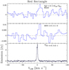 |
Fig. 3 Spectra of the newly tentative detections in the Red Rectangle. For comparison purposes, we also show the 13CO J = 2–1 line in black (Bujarrabal et al. 2013a). The x-axis indicates velocity with respect to the local standard of rest (VLSR) and the y-axis represents the detected flux measured in Jansky. |
 |
Fig. 4 Spectra of the newly detected transitions in 89 Her. For comparison purposes, we also show the 13CO J = 2–1 line in black (Bujarrabal et al. 2013a). The x-axis indicates velocity with respect to the local standard of rest (VLSR) and the y-axis represents the detected flux measured in Jansky. |
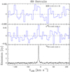 |
Fig. 5 Spectra of the newly tentative detections in 89 Her. For comparison purposes, we also show the 13CO J = 2–1 line in black (Bujarrabal et al. 2013a). The x-axis indicates velocity with respect to the local standard of rest (VLSR) and the y-axis represents the detected flux measured in Jansky. |
4.3 89 Her
We present our results in Tables C.3 and 3, and in Figs. 4 and 5. We detected C18O J = 2–1 and tentatively C17O J = 2–1. We also detected CS J = 3–2 and SiS J = 5–4. All these lines show narrow profiles. Additionally, we tentatively detected HCN J = 1–0. Based on the shape of the observed profiles, we are confident that the emission of these molecules comes from the Keplerian disk and not from the extended outflow.
4.4 HD 52961
We did not detect any emission at the observed frequencies, but we highlight that we present significant upper limits (see Table C.4). We attained a rms of 40,45, and 18 mJ y at 1.3,2, and 3 mm, respectively. The observation at 7 and 13 mm was focused in the detection of SiO and H2O maser emission and we attained a rms of 6 and 31.5 mJ y, respectively.
4.5 IRAS 19157-0257 and IRAS 18123+0511
We focus our mm-wave single-dish observations in the detection of SiO and H2O maser emission at 7 and 13 mm. We have not confirmed the lines in IRAS 19157–0257 and IRAS 18123+0511, but we provide upper limits (we present our results in Tables C.5 and C.6). Some of them clearly improve the rms achieved by previous works by other authors.
We attained an rms in IRAS 19157–0257 of 50, 40, 14 and 34mJy at 2, 3, 7, and 13 mm, respectively. We attain an rms in IRAS 18123+0511 of 90, 55, 30, 17 and 24 mJy at 1.3, 2, 3,7, and 13 mm, respectively.
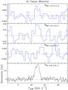 |
Fig. 6 Spectra of the newly tentative detections in AI CMi. For comparison purposes, we also show the 13CO J = 2–1 line in black (Bujarrabal et al. 2013a). The x-axis indicates velocity with respect to the local standard of rest (VLSR) and the y-axis represents the detected flux measured in Jansky. |
4.6 IRAS 19125+0343
We did not detect any emission in IRAS 19125 + 0343 at the observed frequencies, but we highlight that we present significant upper limits (see Table C.7). We have attained a rms of 50, 20, 10, and 23mJy at 1.3, 3, 7, and 13 mm, respectively.
4.7 AI CMi
We present our results in Tables C.8 and 3, and in Figs. 6–8. We detected several lines of thermal SiO: J = 1–0, J = 2–1, and J = 5–4. We also detected SiO isotopic species, 29SiO J = 1–0 and J = 2–1 and 30SiO J = 1–0. We find very intense SiO maser emission for transitions v = 1 J = 1–0 and J = 2–1 and v = 2 J = 1–0. We find wide composite profiles of SO Jn = 22 – 11 and Jn = 65 – 54 and SO2 JKa,Kc = 42,2–41,3. In addition, we detected H2O JKa,Kc = 61,6–52,3 (this line was previously detected, see Sect. 2.7). We detected SiS v = 1 J = 8–7, which, if confirmed, will also be the first detection of this species in AI CMi. However, we note that we did not detect any SiS v = 0 in the observed bands, which is quite surprising but not impossible (SiS v = 1 emission could be due to some weak maser emission).
All the detected thermal lines show composite profiles with a narrow component, in a similar way to what we find in the CO line profiles of this source and in RSct. We think that both sources could be very similar.
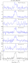 |
Fig. 7 Spectra of the newly detected transitions in AI CMi. For comparison purposes, we also show the 13CO J = 2–1 line in black (Bujarrabal et al. 2013a). The x-axis indicates velocity with respect to the local standard of rest (VLSR) and the y-axis represents the detected flux measured in Jansky. |
4.8 IRAS 20056+1834
We observed this source in 1.3 and 3 mm, resulting in no positive detections and we attained rms values of 45 and 18 mJy, respectively. We also observed this source at 7 mm, where we detected maser emission, SiO v = 1 J = 1–0 and v = 2 J = 1–0 (see Fig. 9). There are no signs of H2O maser emission at 13 mm, but we provide a rms of 27 mJy (see Table C.9 for further details).
The SiO maser emission is centered at approximately –20 km s–1, which is shifted with respect to the CO line profiles by ~10km s–1. This fact is supported by Klochkova et al. (2007), who highlight that velocities measured from lines formed in the photosphere are variable. They reveal differential line shifts up 10 km s–1. Shifts between thermal and maser lines are in any case not usual.
We think that IRAS 20056+1834 could be similar to RSct and AI CMi (a binary system surrounded by a Keplerian disk and an extended outflow that dominates the whole nebula), which would explain the chemical similarities between these sources.
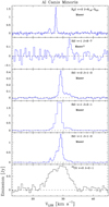 |
Fig. 8 Spectra of the newly maser detections in AI CMi. For comparson purposes, we also show the 13CO J = 2–1 line in black (Bujarrabal et al. 2013a). The x-axis indicates velocity with respect to the local standard of rest (VLSR) and the y-axis represents the detected flux measured in Jansky. |
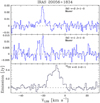 |
Fig. 9 Spectra of the newly maser detections in IRAS 20056+1834. For comparison purposes, we also show the 13CO J = 2–1 line in black (Bujarrabal et al. 2013a). The x-axis indicates velocity with respect to the local standard of rest (VLSR) and the y-axis represents the detected flux measured in Jansky. |
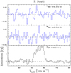 |
Fig. 10 Spectra of the newly tentative detections in R Sct. For comparison purposes, we also show the 13CO J = 2–1 line in black (Bujarrabal et al. 2013a). The x-axis indicates velocity with respect to the local standard of rest (VLSR) and the y-axis represents the detected flux measured in Jansky. |
4.9 RSct
We present our results in Tables C.10 and 3, and in Figs. 10–12. We detected several lines of thermal SiO: J = 1–0, J = 2–1, and J = 5–4. We also detected SiO isotopic species, 29SiO and 30SiO J = 1–0 and J = 2–1. All of them show a narrow profile, which is coincident with the narrow component of the composited CO line profiles. We also detected SiO maser emission for transitions v = 1 J = 1–0 and J = 2–1, v = 2 J = 1–0, and the first-ever detection of the v = 6 J = 1–0. We detected SO JN = 65–54, and the H2O JKa,Kc = 61,6–52,3 maser emission (see Sect. 2.9).
In addition, we also detected HCO+ J = 1–0. This molecule presents weak emission in AGB stars when detected (Bujarrabal et al. 1994b; Pulliam et al. 2011). Furthermore, HCO+ is detected in other standard pPNe, such as CRL 618 (Sánchez Contreras & Sahai 2004), OH 231.8+4.2 (Sánchez Contreras et al. 2015), or M1–92 (Alcolea et al. 2019). The detection of HCO+ in the envelope of R Sct implies that the disk is (partially) ionized. The most probable reason for the presence of HCO+ is that the central star, which is now in the post-AGB phase, can partially ionize the closest and densest regions. These regions correspond to the disk, which would justify the narrow profile of this line (see Fig. 11). Another way to explain the presence of ionized gas could be the presence of shocks, in which the abundance of SO is also favored.
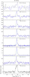 |
Fig. 11 Spectra of the newly detected transitions in R Sct. For comparison purposes, we also show the 13CO J = 2–1 line in black (Bujarrabal et al. 2013a). The x-axis indicates velocity with respect to the local standard of rest (VLSR) and the y-axis represents the detected flux measured in Jansky. |
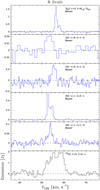 |
Fig. 12 Spectra of the newly maser detections in R Sct. For comparison purposes, we also show the 13CO J = 2–1 line in black (Bujarrabal et al. 2013a). The x-axis indicates velocity with respect to the local standard of rest (VLSR) and the y-axis represents the detected flux measured in Jansky. |
5 Discussion
5.1 Molecular richness
Prior to this work, the presence of molecules other than CO in these objects was practically unknown. We compared our results with standard AGB stars (see e.g., Bujarrabal et al. 1994b), which are the precursors of our objects, representing a homogeneous group that has been studied in great detail and whose envelopes are rich in molecular emission. Additionally, pho-todissociation effects in AGB envelopes only appear in outer layers. The comparison of our results with PNe is more difficult, because these objects present large differences in the molecular gas content (Huggins et al. 1996; Santander-García et al. 2022), which is also present in young PNe (Bujarrabal et al. 1988, 1992). This fact is most likely due to molecular photodis-sociation, which strongly depends on the different evolutionary state of each source (Bachiller et al. 1997a,b; Bublitz et al. 2019; Ziurys et al. 2020). An added difficulty is that there is no complete survey of PNe or young PNe to compare with.
In Fig. 13, we show integrated intensity ratios between the main molecules (SO12, SiO, SiS, CS, and HCN) and CO (13CO J = 2–1 and with 12CO J = 1–0). Additionally, we compare these molecular integrated intensities with infrared emission at 12, 25, and 60 μm (from the IRAS mission, see Neugebauer et al. 1984). We used these three IRAS wavelengths because the shape of the SEDs seems to be strongly related with the evolutionary state of the source (see Fig. A.1 and Kwok et al. 1989; Hrivnak et al. 1989; van der Veen et al. 1995; Oomen et al. 2018). Molecular emission in AGB stars is usually compared to 60 μm, since this band adequately represents the bulk of the circumstel-lar emission. Many pPNe present a bimodal SED with an excess at 25–60 μm and less emission at 5–10 μm, because of a lack of dust characterized by an intermediate temperature. On the contrary, our objects tend to present a significant NIR excess at 12 and 25 μm, and these two bands are probably better tracing most of the nebular material. However, since we want to study the gast-to-dust ratios in our sources and compare them with those in other objects, we needed to use all these three CO-to-IRAS ratios. We always find uncertainties less than ~20% in our ratios, which basically are dominated by that of the integrated intensity of the molecules other than CO (see tables of Appendix C for further details). These uncertainties are too small to be represented in the figures; thus, we note the very broad range (on a logarithmic scale) of the intensity ratios. Our results were compared with molecular emission of AGB stars. Blue and red horizontal lines represent averaged values of the molecular emission for O- and C-rich AGB stars, respectively. We note that the emission of molecules other than CO in our sources is low. This fact is especially remarkable in those sources which are dominated by their rotating disk (AC Her and the Red Rectangle) or intermediate cases (such as 89 Her).
In Fig. 14, we show, 12CO - to - IR and 13CO - to - IR ratios for the integrated intensity of J = 2–1 and J = 1–0. For transitions compared with the IR fluxes, the 12CO emission is relatively low with respect to the levels exhibited by AGB stars. Again, we find two subclasses in our sample. Those sources in which the Keplerian disk dominates the nebula tend to present a lower relative intensity of 12CO compared to the outflow-dominated ones. On the contrary, we do not see this effect in 13CO emission, which seems to be relatively intense compared with 12CO and comparable to that from AGB stars. The difference found in this ratio in the disk- and the outflow-dominated sources could be due to higher optical depths in the 12CO J = 2–1 line. The emission of the outflow-dominated sources comes from relatively extensive and very diffuse areas, thus they are expected to show low optical depths in the 12CO J = 2–1 line. For example, in the case of RSct, the emitting area exceeds 2× 1017cm. However, in the case of the very well known disk-dominated sources, such as AC Her, the emitting area does not exceed 2 × 1016 cm, which means that it is ten times smaller than in the case of R Sct. Thus, based on this discussion and the results (see Fig. 13), we find a real difference in the relative abundances that seems to confirm that the outflow-dominated sources present relative higher 13CO abundance. This fact was previously noted in R Sct, which is an outflow-dominated source (Gallardo Cava et al. 2021; Bujarrabal et al. 1990), where a very low 12C/13C ratio was reported.
 |
Fig. 13 Ratios of integrated intensities of molecules (SO, SiO, SiS, CS, and HCN) and infrared emission (12, 25, and 60 μm) in binary post-AGB stars. Upper limits are represented with empty circles. Blue and red lines represent the averaged values for O- and C-rich AGB CSEs. Sources are ordered by increasing outflow dominance and enumerated as follows: 1 – AC Her, 2 – Red Rectangle, 3 – 89 Her, 4 – HD 52961, 5 – IRAS 19157–0257, 6 – IRAS 18123+0511, 7 – IRAS 19125+0343, 8 – AI CMi, 9 – IRAS 20056+1834, and 10 – R Sct. Sources 1 and 2 are disk-dominated binary post-AGB stars, sources 6–10 are outflow-dominated, while sources 3 and 4, and 5 are intermediate cases. We note the broad range (on a logarithmic scale) of intensity ratios. We always find uncertainties lower than ~20% in these ratios, which are basically dominated by that of the integrated intensity of the molecules other than CO (see main text for details). |
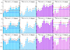 |
Fig. 14 Ratios of integrated intensities of 12CO (blue) and 13CO (purple) J = 2–1 and J = 1–0 and infrared emission (12, 25, and 60 μm) in binary post-AGB stars. Blue and red lines represent the averaged values for O- and C-rich AGB CSEs. Sources are are ordered by increasing outflow dominance and enumerated as follows: a – HR 4049, b – DY Ori, 1 – AC Her, 2 – Red Rectangle, 3 – 89 Her, 4 – HD 52961, 5 – IRAS 19157–0257, 6 – IRAS 18123+0511, 7 – IRAS 19125+0343, 8 – AI CMi, 9 – IRAS 20056+1834, and 10 – R Sct. Souces a and b are not included in this mm-wave survey. Sources 1, 2, a, and b are disk-dominated binary post-AGB stars, sources 6 to 10 are outflow-dominated, and sources 3, 4, and 5 are intermediate cases. We note the broad range (on a logarithmic scale) of intensity ratios. We find uncertainties less than ~10% in these ratios, which are basically dominated by that of the integrated intensity of CO (see Bujarrabal et al. 2013a). |
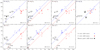 |
Fig. 15 Integrated intensities of pairs of molecular transitions in binary post-AGB stars (black), as well in O- and C-rich stars (blue and red). Blue and red lines represent the averaged values for O- and C-rich AGB CSEs (only in the case of detections). The X and Y axes represent the integrated intensities of the observed transitions in logarithmic scale and units of Jy km s-1. The upper limits are represented bv arrows. |
5.2 Discrimination between O- and C-rich envelopes
In general, evolved stars can be classified as O- and C-rich according to their relative O / C elemental abundance. It is known that this difference, even if the O/C abundance ratio is not always shown to vary much from 1, has important effects on the molecular abundances. SiO, SO are O-bearing molecules and their lines are much more intense in O-rich envelopes than in the C-rich ones, while HCN and CS (HC3N and HNC) are C-bearing molecules (but also SiS), whose lines are more intense in C-rich envelopes than in O-rich (see e.g. Bujarrabal et al. 1994b,a). Additionally, SiO maser emission is detected in M- and S-type AGB stars, and H2O maser emission is only seen in M-type stars. In any case, SiO and H2O maser emission is seen exclusively towards O-rich envelopes (Kim et al. 2019). The analysis of integrated intensities of pairs of molecular transitions is very useful to distinguish between O- and C-rich environments (see Fig. 15). Integrated intensities are larger for O-rich than for C-rich objects when an O-bearing molecule is compared with a C-bearing one. Our results are compared with CSEs around AGB stars, which are deeply studied objects and they are prototypical of environments rich in molecules (for this comparison, AGB data is taken from Bujarrabal et al. 1994b,a, which represent a wide sample of CSEs around evolved stars in the search molecules other than CO). In Fig. 15, blue and red lines represent averaged values for these ratios in O- and C-rich AGB CSEs, respectively.
In the case of AI CMi and R Sct, the integrated intensities of SO and SiO compared with C-bearing molecules are remarkably larger than for C-rich evolved stars. Both sources present SiO and H2O maser emission (AI CMi also presents OH maser emission according to te Lintel Hekkert et al. 1991). Additionally, the IR spectra of R Sct is mainly dominated by H2O emission (Matsuura et al. 2002; Yamamura et al. 2003). These facts lead us to classify AI CMi and R Sct as O-rich. The Red Rectangle presents O- and C-bearing molecular emission. This case will be examined in more detail in Sect. 5.4, but according to Fig. 15 and the tentative H2O maser detection, we catalog the Red Rectangle as O-rich too. There are no signs of O-bearing molecules in 89 Her and we detected HCN, CS, and SiS, so the chemistry of this source is absolutely compatible with a C-rich nebula. Finally, we did not detect any thermal SiO emission in IRAS 20056+1834, but we have clearly confirmed the existence of SiO maser emission and tentative SiO maser emission in AC Her (see Sects. 4.1 and 4.8), which is exclusive of O-rich environments.
Based on the integrated intensities ratios in Fig. 15 and the maser detection of O-bearing molecules, we can classify some of our sources as O- / C-rich (see a summary of our results in Table 5). 89 Her presents a O/C<1 chemistry. On the contrary, AC Her, AI CMi, IRAS 20056+1834, and R Sct present a O/C> 1 chemistry. The chemistry of the Red Rectangle could be uncertain, but we also classified this source as O-rich (see Sect. 5.4 for further details). In any case, we recall that our sources are still poorly studied and that additional work, both observational and theoretical, is needed to confirm our findings on the general chemistry of these sources.
5.3 Abundance estimates
The methodology to estimate abundances is similar to that used in Bujarrabal et al. (2001); Quintana-Lacaci et al. (2007); Bujarrabal et al. (2013a) and is described in Appendix B in detail. This procedure assumes optically thin emission, which is justified in our case, because the molecular lines present very weak emission (see Sect. 5.1). To estimate the characteristic rotational temperature (Trot), it is necessary to observe (at least) two transitions of the same molecule. We apply this procedure, using Eq. (B.11), to AI CMi and RSct for SiO and its rare isotopic substitutions. We assume nebular masses derived from previous works (see Table 1, Bujarrabal et al. 2013a; Gallardo Cava et al. 2021).
After computing the abundances, we checked that our optically thin assumption is valid. We estimated the line opacities expected for the derived values of abundances and Trot. These values are shown in Table B.1. We can see that in all cases, τ≪1.
We estimate the rotational temperature (Trot) from the observed line ratios. Different values of the abundance are calculated for each transition as a function of Trot (see Appendix B for further details). The minimum relative difference of the abundances yields the best-fit rotational temperature (see Fig. 16 and Eqs. (B.12) and (B.13)). For SiO, the best-fit Trot is 8 and 14 K in AI CMi and R Sct, respectively. We find relaive errors lower than 5% between the integrated line intensity and the predicted one derived from Eq. (B.11) (see Fig. 16 bottom). This relative error between the integrated intensity line and the predicted one considerably increases if we consider small variations with respect to our best-fit Trot. We can assume the rotational temperature of SiO for 29SiO and 30SiO, as well as for HCO+, because the lines show similar excitation properties and line profiles (see Fig. 11).
We see that most of the molecular line shapes are very similar to that of the CO lines (except the masers, whose lines have not been considered for the calculation of abundances; see Sect. 4). We estimated the molecular mass of the envelopes of these sources based on the CO lines. Therefore, we can calcuate relative abundances of molecules other than CO assuming that their emission comes from the same molecule-rich zone for which mass values were derived. This is not the case of R Sct, whose thermal emission of molecules is narrower than that of CO. We think that the emission of these molecules very probably comes from the rotating disk and the high density region of the outflow (see Figs. 10 and 11). We present abundance calculations for the total nebular mass, 〈X〉, and for that of the central region of the nebula, 〈Xc〉, which represents the rotating gas and the innermost regions of the outflow. In other words, 〈X〉 represents the relative abundance considering that the species are located in the whole nebula, while 〈Xc〉 is the value obtained assuming that the species are located only in the densest part of the nebula. According to our previous reasoning, for R Sct our best option is to compute relative abundances with respect to the CO mass in these central regions, which in this case account for 40% of the total nebular mass. The shapes of the SiO, SO, and SO2 line profiles of AI CMi are very similar to that in CO (see Fig. 7); therefore we think that the molecular emission of AI CMi must arise from the entire nebula. We recall that in any case, these estimates are uncertain by a factor of 2 (in addition to uncertainties for other reasons) in view of the assumed fraction of involved material. To estimate relative abundances assuming other fractions of the mass of the molecular rich component, f, with respect to the total nebular mass, we only need to multiply 〈X〉 by f−1.
In the case of the Red Rectangle and 89 Her there is only one detected transition per molecule, so we can only make very crude estimations of the abundance by assuming the obtained Trot of SiO for AI CMi and R Sct and the nebular masses derived from previous works (Bujarrabal et al. 2016; Gallardo Cava et al. 2021). We also estimated abundances for the whole nebula and for the inner regions: in the case of the Red Rectangle ~90% is located in the disk; in the case of 89 Her, 60% of the total molecular mass corresponds to the rotating disk and the inner regions of the outflow. Based on the same reasoning as in the case of AI CMi, our best option for Red Rectangle and 89 Her is to consider the abundance corresponding to the total molecular mass.
The calculated abundances for AI CMi, R Sct, Red Rectangle, and 89 Her can be seen in Table 6 (we also show estimated optical depths in Table B.1). We note the very low abundances we deduce, compared with standard AGB stars, which reinforces our conclusion, set out in Sect. 5.1. We can see again how the presence of molecules in disk-dominated or intermediate sources is much weaker than that in outflow-dominated ones.
Chemistry of the envelopes around binary post-AGB stars observed in this paper.
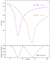 |
Fig. 16 Top: variations of the relative difference of the abundances produced by the line-ratio method as a function of the rotational temperature Δd (Trot) in the case of AI CMi and R Sct. The minimum relative difference corresponds to the best-fit value of Trot. This procedure can only be performed for those sources in which several transitions of the same molecule have been observed. See text and Appendix B for more details. Bottom: variations of the relative error of the observational integrated intensity line and the predicted one as a function of the rotational temperature for SiO J = 5–4. The predicted integrated intensity lines are derived from Eq. (B.11) using the estimated abundance and rotational temperature. |
Abundances estimated.
5.4 Dual nature of the Red Rectangle
The chemistry of these kinds of objects was barely known even for the case of the Red Rectangle, which is by far the best-studied object. Apart from CO, Bujarrabal et al. (2016) discovered H13CN J = 4−3, CI J = 2-1 and J = 1−0, and C IIJ = 2−1. In this work, we detected C17O and C18O J = 2−1, and SO JN = 66−54, and we also tentatively detected HCN J = 1−0 and H2O JKa,Kc = 61,6−52,3. Both SO and H2O (at 22 GHz) are good tracers of O-rich environments (see Sect. 5.2). Additionally, we attained very significant SiO and SiS emission upper limits. We estimated the upper limits on the abundance of these molecules following the method described in Appendix B, assuming a 3σ limit for intensity and integrated intensity lines and Trot = 11 ± 3 K (see Table C.2 and Sect. 5.3). We find 〈X〉sio < (5.9 ± 0.8) × 10−9 and 〈X〉sis < (2.3 ± 0.1) × 10−10 (see Table 6 for comparison).
The solar abundance of Si is ~6.5 × 10⁻⁵ (see e.g., Asplund et al. 2021). In the case of O-rich AGB stars, SiO abundances vary in between 4 × 10⁻⁵ and 5 × 10⁻⁶, depending on the state of depletion onto dust grains (Verbena et al. 2019). These values for the abundances are considerably larger than the estimated upper limits for SiO and SiS. Taking into account the fact that the abundance of SiO decreases as grains of dust are formed (Gobrecht et al. 2016), it seems that the depletion process is very efficient, at least in the Red Rectangle and practically all Si could be depleted onto the grains. This conclusion is reinforced if we consider that the molecular emission of the Red Rectangle practically comes from the Keplerian disk, where depletion should be more effective than in the case of an expanding and very large envelope, as for AGB stars (since, in a rotating disk structure, there is more time for the grains to grow bigger).
C II emission must have its origin in the PDR, because it is the best tracer of these regions. C I is also very often associated with PDRs. The presence of H13CN is also compatible with the development of a PDR in the dense disk region that is close to the stellar system, which is a binary system with a secondary star and an accretion disk that emits in the UV (Witt et al. 2009; Thomas et al. 2013). The UV emission can excite a zone in between the H II region and the Keplerian molecule-rich disk (Bujarrabal et al. 2016). According to models of the PDR chemistry, the origin of the HCN can be the photoinduced formation (Agúndez et al. 2008) and it has been detected in the innermost regions of several disks around young stars. This fact is also consistent with the detection of HCN (see Fig. 2).
In conclusion, we think that the Red Rectangle most likely presents a O-rich gas chemistry, but it also presents a PDR in the innermost region of the Keplerian disk. The UV excess can explain the detection of HCN (and H13CN, C I, and C II) together with PAHs, even in an O-rich environment. We note that this is the typical situation in star-forming regions and that these are thought to be O-rich despite the presence of C-bearing species, including PAHs.
5.5 Isotopic ratios
5.5.1 17O/18O
Complex stellar evolution models reveal that the 17O/18O ratio remains approximately constant over the entire thermally pulsating AGB phase, and the initial stellar mass (Mi) can be directly obtained from this ratio (De Nutte et al. 2017). We can estimate the 17O/18O abundance ratio using the C17O and C18O J = 2-1 line intensities corrected for different beam widths and Einstein coefficients, because both molecules present almost identical radial depth dependence (Visser et al. 2009), low optical depths, and very similar and easily predictable excitations conditions.
We applied this criterium to our entire sample. According to our results in Tables C.2 and C.3, we estimate the abundance ratio for the Red Rectangle and 89 Her, respectively. Initial stellar masses for the post-AGBs stars are shown in Table 7. We additionally show the total stellar mass (MTc) derived from the Keplerian dynamics and the total nebula mass (Mneb), which includes the mass of the rotating disk and outflow (see Bujarrabal et al. 2016; Gallardo Cava et al. 2021). We note that the derived values of Mi are consistent with MTc, which must be higher because of the presence of a companion. The 17O / 18O ratio for 89 Her is typical of a O-rich object, while its chemistry is typical of C-rich environments. We note that abundance models are set up for single stars and not for binary stars where it is very likely that mass transfer happen after the results of the evolution of the individual stars.
5.5.2 12CO/13CO
For our binary post-AGB stars, we find a 12CO / 13CO integrated-line ratio (see Fig. 17), with amean value of 4.1 and a standard deviation of 1.4 for the transition J = 1−0 (3.3 ± 0.9 for J = 2−1). This ratio can be compared with intensity line ratios of other post-AGB stars, in which we find 10.4 ± 7.6 (see Palla et al. 2000; Balser et al. 2002; Sanchez Contreras & Sahai 2012). Although these ratios must be corrected for different beam widths, Einstein coefficients, and opacity (especially for the 12CO J = 2−1 lines), our objects seem to present higher 13CO abundance compared with other post-AGB stars. As stated before, the 12CO / 13CO abundance ratio was previously derived for seven of our sources (see Bujarrabal et al. 2016, 2017, 2018; Gallardo Cava et al. 2021). From these works, we are able to find a 12CO / 13CO mean value of 8.6 ± 2.4. We can compare this ratio to that of AGB stars: 12.7 ± 5.8, 28.0 ± 16.2, and 31.3 ± 28.2 for M-, S-, and C-type stars, respectively (see Ramstedt & Olofsson 2014). Again, our objects present a higher 13CO abundance compared with any sub-class of AGB stars, and are only similar to those of M-type stars presenting very low abundance ratios.
Our results support the suggestion by Ramstedt & Olofsson (2014) that the binary nature of the sources is the origin of these very low 12CO / 13CO ratios found in other post-AGB stars, because all our sources are bona-fide binary systems in which a strong interaction between the stars and the circumbinary disk is expected (Van Winckel 2003).
O-isotopic abundance ratio, initial stellar mass estimation compared with the central total stellar mass and the total nebula mass.
6 Conclusions
We present a very deep survey of mm-wave lines in binary post-AGB stars, which is the first systematic study of this kind. We show our single-dish observational results in Sect. 4, where detected lines together with very relevant upper limits are presented.
Our molecular study allows us to verify that our sources present lower molecular intensities of all species than those typical of AGB sources (see Sect. 5.1). This fact is very significant in those binary post-AGB stars for which the Keplerian disk is the dominant component (i.e., the Red Rectangle and AC Her) or at least it has a significant weight in the whole nebula, such as 89 Her. This lower molecular richness is also present in CO, and it is again very remarkable in disk-dominated sources. On the other hand, we find some overabundance of 13CO, especially in our outflow-dominated objects.
Our analysis of integrated intensities ratios of pairs of molecules other than CO leads us to classify the chemistry of (some of) our sources as C- or O-rich (see Sect. 5.2). We cataloged the nebulae around AC Her, the Red Rectangle, AI CMi, RSct, and IRAS 20056+1834 as O-rich environments. On the contrary, the nebula around 89 Her is a C-rich environment.
We estimated abundances of the different species using the method described in detail in Appendix B. As expected, our results reveal that our sources present very low abundances in molecules other than CO (see Sect. 5.3) compared with standard evolved stars. The chemistry of these objects is yet to be studied from the theoretical point of view.
We also studied the isotopic ratios of our sources (see Sect. 5.5). We deduced the initial stellar mass for the Red Rectangle and 89 Her via the 17O/18O ratio, which is consistent with the current central total stellar mass derived of our mm-wave interferometric maps and models (see Table 7). We studied the 12CO / 13CO ratios and we find that our sources, which are all post-AGB stars, tend to present an overabundance of 13CO compared to AGB and other post-AGB stars.
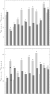 |
Fig. 17 Ratios of integrated intensities of 12CO /13CO in binary post-AGB stars in light grey. We also show line-peak ratios in dark grey (J = 2−1 at top; J = 1−0 at Bottom). Sources are ordered by outflow dominance and enumerated as follows: a – HR 4049, b – DY Ori, 1 – AC Her, 2 – Red Rectangle, 3 – 89 Her, 4 – HD 52961, 5 – IRAS 19157-0257, 6 – IRAS 18123+0511, 7 – IRAS 19125+0343, 8 – AI CMi, 9 – IRAS 20056+1834, and 10 – RSct. Sources a and b are not included in this mm-wave survey. Sources 1, 2, a, and b are disk-dominated binary post-AGB stars, sources 6 to 10 are outflow-dominated, and sources 3, 4, and 5 are intermediate cases. |
Acknowledgements
We are grateful to the anonymous referee for the relevant recommendations and comments. This work is based on observations carried out with the 30 m IRAM telescope. IRAM is supported by INSU/CNRS (France), MPG (Germany), and IGN (Spain). This work is also based on observations with the 40 m Yebes telescope of the National Geographic Institute of Spain (IGN) at Yebes Observatory. Yebes Observatory thanks the ERC for funding support under grant ERC-2013-Syg-610256-NANOCOSMOS. This work is part of the AxiN and EVENTs / NEBULAE WEB research programs supported by Spanish AEI grants AYA 2016-78994-P and PID2019-105203GB-C21, respectively. IGC acknowledges Spanish MICIN the funding support of BES2017-080616.
Appendix A Additional figures
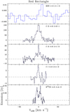 |
Fig. A.1 Spectra for HCN J = 1 − 0 detected in the Red Rectangle. We also show other PDR-tracing lines in black taken from Bujarrabal et al. (2016). The x-axis indicates velocity with respect to the local standard of rest (VLSR) and the y-axis represents the emitted emission measured in Jansky. |
In this Appendix, we show other relevant figures. In Fig. A.2 we present our tentative detection of HCN J = 1 − 0 in the Red Rectangle. We also show in black H13CN J = 1 − 0, CI J = 1 − 0, C II J = 1 − 0, and C II J = 2 − 1 (ALMA data taken from Bujarrabal et al. 2016).
In Fig. A.1, we show the color-color diagram where we represent [25]–[60] versus [12]–[25] IRAS colors. We also show the regions populated stars with similar properties (see van der Veen & Habing 1988, for more details). These kinds of plots show the evolutionary sequence of AGB/post-AGB stars. We note that the sources of this work, the binary post-AGB stars, are in between of AGB stars and pPNe and young PNe, which confirms the nature of our sources.
Appendix B Estimation of abundances: Methodology
In this appendix, we show in detail the procedure used for the estimation of the abundance of molecules with more than one detected transition, assuming optically thin emission. In our case, we use this procedure to estimate the abundance of SiO for R Sct and AI CMi (see Sects. 4.7 and 4.9).
The observed main-beam temperature for a specific molecular transition is expressed as:
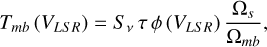 (B.1)
(B.1)
where τ is the characteristic optical depth, ϕ (VLSR) is the normalized line profile in terms of Doppler-shifted velocity, and Ωs and Ωmb are the solid angles subtended by the source and the telescope main beam, respectively. These are given by:
 (B.2)
(B.2)
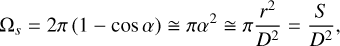 (B.3)
(B.3)
where θHPBW is the Half Power Beam Width (HPBW) and α is the angle formed by the radius r of the source from the observer at a distance D. In the limit of small angle α, we assume that  and
and  . The ratio
  is known as the dilution factor, which can only take values lower than 1 (for Ωs larger than Ωmb, namely, spatially resolved sources, the dilution factor is set to one).
The source function is given by:
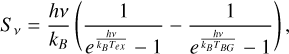 (B.4)
(B.4)
where Tex is the excitation temperature of the transition and TBG = 2.7 K is the background temperature. The optical depth, τ, can be expressed as:
 (B.5)
(B.5)
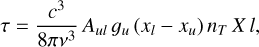
where X is the abundance of the studied molecule, nT is the total number density of particles, and l is the typical length of the source along the line of sight. The subindexes u and l represent the upper and lower levels of the transition, respectively. Aul; is the Einstein coefficient of the transition, gu is the statistical weight of the upper limit expressed as
 (B.6)
(B.6)
and xu and xl are:
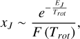 (B.7)
(B.7)
where E is the energy of the considered levels, in terms of temperature, and for simple linear rotors it can be calculated as:
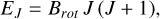 (B.8)
(B.8)
where Brot is the rotational constant of the molecule. Trot is the rotational temperature and it is defined as the typical value or average of the excitation temperatures of the relevant rotational lines (in our case, low-J transitions) and is used to approximately calculate the partition function F (Trot):
 (B.9)
(B.9)
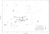 |
Fig. A.2 Diagram of [25]–[60] vs. [12]–[25] IRAS colors. The IRAS color-color diagram is divided in different regions where sources with similar characteristics are located (see van der Veen & Habing 1988, for details). Standard AGB stars are represented with blue triangles (O-rich) and red squares (C-rich), pre-planetary and young planetary nebulae are represented with purple circles and the binary post-AGB stars of this work are shown with black circles. |
We can express τ (Eq. B.5) in terms of the mass, taking into account:
 (B.10)
Integrating (Eq. B.1) in terms of velocity, we get:
 (B.11)
We estimate Trot from the line intensity ratio for those molecules, where we observed more than one transition (SiO, see Sect. 4). We calculated several abundances for the different transitions (XJ=u−l, X′J=u′−l′) of the same molecule and then we estimated the parameter di for each pair of transitions:
 (B.12)
We can quantify the quality of the fit through the parameter Δd(Trot):
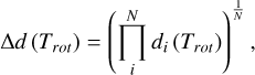 (B.13)
where N indicates the number of transitions used in each case. The value of Trot that minimizes the value of Δd (Trot) in Eq. B.13 will be the best-fit rotational temperature (see Fig. 16). Finally, knowing Trot, we can estimate the abundance through Eq. B.11.
Additionally, using Eq. B.1, we can express the optical depth as:
 (B.14)
and we can express the averaged optical depth over the beam of the telescope as:
 (B.15)
The averaged optical depths values can be seen in Table B.1. We note that these  values are very small, and that for the dilution factors expected for our sources, always lower than 10 (see Gallardo Cava et al. 2021; Bujarrabal et al. 2016, 2013a), implying that the lines are optically thin (τ < 1). Additionally, we note that always compare our detections with 13CO J = 2 − 1, which is an optically thin line and shows a similar beam size.
Optical depths estimated.
Appendix C Tables
In this appendix, we show the most relevant line parameters for AC Her, the Red Rectangle, 89 Her, HD 52961,IRAS 19157−0257, IRAS 18123+0511, IRAS 19125+0343, AI CMi, IRAS 20056+1834, and RSct (see Sect. 4). We note that most of the sources have been observed in the 1.3, 2, 3, 7, and 13 mm bands (see Table 2).
Radio molecular line survey of AC Her.
Radio molecular line survey of the Red Rectangle.
Radio molecular line survey of 89 Her.
Radio molecular line survey of HD 52961.
Radio molecular line survey of IRAS 19157-0257.
Radio molecular line survey of IRAS 18123+0511.
Radio molecular line survey of IRAS 19125+0343.
Radio molecular line survey of AI CMi.
Radio molecular line survey of IRAS 20056+1834.
Radio molecular line survey of R Sct.
References
- Agúndez, M., Cernicharo, J., & Goicoechea, J. R. 2008, A&A, 483, 831 [NASA ADS] [CrossRef] [EDP Sciences] [Google Scholar]
- Alcolea, J., Agúndez, M., Bujarrabal, V., et al. 2019, IAU Symp., 343, 343 [NASA ADS] [Google Scholar]
- Arkhipova, V. P., Ikonnikova, N. P., Esipov, V. F., & Komissarova, G. V. 2017, VizieR Online Data Catalog: J/PAZh/43/460 [Google Scholar]
- Asplund, M., Amarsi, A. M., & Grevesse, N. 2021, A&A, 653, A141 [NASA ADS] [CrossRef] [EDP Sciences] [Google Scholar]
- Bachiller, R., Forveille, T., Huggins, P. J., & Cox, P. 1997a, A&A, 324, 1123 [Google Scholar]
- Bachiller, R., Fuente, A., Bujarrabal, V., et al. 1997b, A&A, 319, 235 [NASA ADS] [Google Scholar]
- Balser, D. S., McMullin, J. P., & Wilson, T. L. 2002, ApJ, 572, 326 [NASA ADS] [CrossRef] [Google Scholar]
- Bublitz, J., Kastner, J. H., Santander-García, M., et al. 2019, A&A, 625, A101 [NASA ADS] [CrossRef] [EDP Sciences] [Google Scholar]
- Bujarrabal, V. 2006, IAU Symp., 234, 193 [NASA ADS] [CrossRef] [Google Scholar]
- Bujarrabal, V., Gomez-Gonzalez, J., Bachiller, R., & Martin-Pintado, J. 1988, A&A, 204, 242 [Google Scholar]
- Bujarrabal, V., Alcolea, J., & Bachiller, R. 1990, A&A, 234, 355 [NASA ADS] [Google Scholar]
- Bujarrabal, V., Alcolea, J., & Planesas, P. 1992, A&A, 257, 701 [NASA ADS] [Google Scholar]
- Bujarrabal, V., Fuente, A., & Omont, A. 1994a, A&A, 285, 247 [NASA ADS] [Google Scholar]
- Bujarrabal, V., Fuente, A., & Omont, A. 1994b, ApJ, 421, L47 [NASA ADS] [CrossRef] [Google Scholar]
- Bujarrabal, V., Castro-Carrizo, A., Alcolea, J., & Sanchez Contreras, C. 2001, A&A, 377, 868 [NASA ADS] [CrossRef] [EDP Sciences] [Google Scholar]
- Bujarrabal, V., Castro-Carrizo, A., Alcolea, J., & Neri, R. 2005, A&A, 441, 1031 [NASA ADS] [CrossRef] [EDP Sciences] [Google Scholar]
- Bujarrabal, V., Alcolea, J., Van Winckel, H., Santander-García, M., & Castro-Carrizo, A. 2013a, A&A, 557, A104 [NASA ADS] [CrossRef] [EDP Sciences] [Google Scholar]
- Bujarrabal, V., Castro-Carrizo, A., Alcolea, J., et al. 2013b, A&A, 557, L11 [CrossRef] [EDP Sciences] [Google Scholar]
- Bujarrabal, V., Castro-Carrizo, A., Alcolea, J., & Van Winckel, H. 2015, A&A, 575, L7 [CrossRef] [EDP Sciences] [Google Scholar]
- Bujarrabal, V., Castro-Carrizo, A., Alcolea, J., et al. 2016, A&A, 593, A92 [NASA ADS] [CrossRef] [EDP Sciences] [Google Scholar]
- Bujarrabal, V., Castro-Carrizo, A., Alcolea, J., et al. 2017, A&A, 597, L5 [NASA ADS] [CrossRef] [EDP Sciences] [Google Scholar]
- Bujarrabal, V., Castro-Carrizo, A., Van Winckel, H., et al. 2018, A&A, 614, A58 [NASA ADS] [CrossRef] [EDP Sciences] [Google Scholar]
- Cernicharo, J., Guélin, M., & Kahane, C. 2000, A&AS, 142, 181 [NASA ADS] [CrossRef] [EDP Sciences] [Google Scholar]
- Cernicharo, J., Agúndez, M., & Guélin, M. 2011, in The Molecular Universe, eds. J. Cernicharo, & R. Bachiller (Cambridge: Cambridge University Press), 280, 237 [NASA ADS] [Google Scholar]
- Deguchi, S., Sakamoto, T., & Hasegawa, T. 2012, PASJ, 64, 4 [NASA ADS] [Google Scholar]
- De Nutte, R., Decin, L., Olofsson, H., et al. 2017, A&A, 600, A71 [NASA ADS] [CrossRef] [EDP Sciences] [Google Scholar]
- de Ruyter, S., van Winckel, H., Maas, T., et al. 2006, A&A, 448, 641 [NASA ADS] [CrossRef] [EDP Sciences] [Google Scholar]
- de Vicente, P., Bujarrabal, V., Díaz-Pulido, A., et al. 2016, A&A, 589, A74 [CrossRef] [EDP Sciences] [Google Scholar]
- Dominik, C., Dullemond, C. P., Cami, J., & van Winckel, H. 2003, A&A, 397, 595 [NASA ADS] [CrossRef] [EDP Sciences] [Google Scholar]
- Engels, D. 1979, A&AS, 36, 337 [NASA ADS] [Google Scholar]
- Engels, D., & Lewis, B. M. 1996, A&AS, 116, 117 [NASA ADS] [Google Scholar]
- Gallardo Cava, I., Gómez-Garrido, M., Bujarrabal, V., et al. 2021, A&A, 648, A93 [NASA ADS] [CrossRef] [EDP Sciences] [Google Scholar]
- Gehrz, R. 1989, IAU Symp., 135, 445 [Google Scholar]
- Gielen, C., van Winckel, H., Min, M., Waters, L. B. F. M., & Lloyd Evans, T. 2008, A&A, 490, 725 [NASA ADS] [CrossRef] [EDP Sciences] [Google Scholar]
- Gielen, C., Bouwman, J., van Winckel, H., et al. 2011a, A&A, 533, A99 [NASA ADS] [CrossRef] [EDP Sciences] [Google Scholar]
- Gielen, C., Cami, J., Bouwman, J., Peeters, E., & Min, M. 2011b, A&A, 536, A54 [NASA ADS] [CrossRef] [EDP Sciences] [Google Scholar]
- Gobrecht, D., Cherchneff, I., Sarangi, A., Plane, J. M. C., & Bromley, S. T. 2016, A&A, 585, A6 [NASA ADS] [CrossRef] [EDP Sciences] [Google Scholar]
- Gómez, Y., Moran, J. M., & Rodriguez, L. F. 1990, Rev. Mex. Astron. Astrofis., 20, 55 [Google Scholar]
- Guilloteau, S., & Dutrey, A. 1998, A&A, 339, 467 [Google Scholar]
- Guilloteau, S., Di Folco, E., Dutrey, A., et al. 2013, A&A, 549, A92 [NASA ADS] [CrossRef] [EDP Sciences] [Google Scholar]
- Hillen, M., Verhoelst, T., Van Winckel, H., et al. 2013, A&A, 559, A111 [NASA ADS] [CrossRef] [EDP Sciences] [Google Scholar]
- Hillen, M., Menu, J., Van Winckel, H., et al. 2014, A&A, 568, A12 [NASA ADS] [CrossRef] [EDP Sciences] [Google Scholar]
- Hillen, M., Van Winckel, H., Menu, J., et al. 2017, A&A, 599, A41 [NASA ADS] [CrossRef] [EDP Sciences] [Google Scholar]
- Hrivnak, B. J., Kwok, S., & Volk, K. M. 1989, ApJ, 346, 265 [Google Scholar]
- Huggins, P. J., Bachiller, R., Cox, P., & Forveille, T. 1996, A&A, 315, 284 [Google Scholar]
- Jura, M. 2003, ApJ, 582, 1032 [Google Scholar]
- Jura, M., Turner, J., & Balm, S. P. 1997, ApJ, 474, 741 [NASA ADS] [CrossRef] [Google Scholar]
- Kalaee, M. J., & Hasanzadeh, A. 2019, New Astron., 70, 57 [NASA ADS] [CrossRef] [Google Scholar]
- Kim, J., Cho, S. H., Bujarrabal, V., et al. 2019, MNRAS, 488, 1427 [Google Scholar]
- Kiss, L. L., Derekas, A., Szabó, G. M., Bedding, T. R., & Szabados, L. 2007, MNRAS, 375, 1338 [NASA ADS] [CrossRef] [Google Scholar]
- Klochkova, V. G., Panchuk, V. E., Chentsov, E. L., & Yushkin, M. V. 2007, Astrophys. Bull., 62, 217 [NASA ADS] [CrossRef] [Google Scholar]
- Kluska, J., Van Winckel, H., Hillen, M., et al. 2019, A&A, 631, A108 [NASA ADS] [CrossRef] [EDP Sciences] [Google Scholar]
- Kwok, S., Volk, K. M., & Hrivnak, B. J. 1989, ApJ, 345, L51 [Google Scholar]
- Lebre, A., & Gillet, D. 1991, A&A, 246, 490 [NASA ADS] [Google Scholar]
- Lewis, B. M. 1997, ApJS, 109, 489 [NASA ADS] [CrossRef] [Google Scholar]
- Liu, J., & Jiang, B. 2017, AJ, 153, 176 [NASA ADS] [CrossRef] [Google Scholar]
- Massalkhi, S., Agúndez, M., Cernicharo, J., & Velilla-Prieto, L. 2020, A&A, 641, A57 [NASA ADS] [CrossRef] [EDP Sciences] [Google Scholar]
- Matsuura, M., Yamamura, I., Zijlstra, A. A., & Bedding, T. R. 2002, A&A, 387, 1022 [NASA ADS] [CrossRef] [EDP Sciences] [Google Scholar]
- Matsuura, M., Barlow, M. J., Zijlstra, A. A., et al. 2009, MNRAS, 396, 918 [NASA ADS] [CrossRef] [Google Scholar]
- Neugebauer, G., Habing, H. J., van Duinen, R., et al. 1984, ApJ, 278, L1 [NASA ADS] [CrossRef] [Google Scholar]
- Olofsson, H., Eriksson, K., Gustafsson, B., & Carlstroem, U. 1993, ApJS, 87, 305 [NASA ADS] [CrossRef] [Google Scholar]
- Oomen, G.-M., Van Winckel, H., Pols, O., et al. 2018, A&A, 620, A85 [NASA ADS] [CrossRef] [EDP Sciences] [Google Scholar]
- Oomen, G.-M., Van Winckel, H., Pols, O., & Nelemans, G. 2019, A&A, 629, A49 [NASA ADS] [CrossRef] [EDP Sciences] [Google Scholar]
- Palla, F., Bachiller, R., Stanghellini, L., Tosi, M., & Galli, D. 2000, A&A, 355, 69 [NASA ADS] [Google Scholar]
- Pardo, J. R., Cernicharo, J., Goicoechea, J. R., Guélin, M., & Asensio Ramos, A. 2007, ApJ, 661, 250 [NASA ADS] [CrossRef] [Google Scholar]
- Park, J. A., Cho, S.-H., Lee, C. W., & Yang, J. 2008, AJ, 136, 2350 [NASA ADS] [CrossRef] [Google Scholar]
- Pulliam, R. L., Edwards, J. L., & Ziurys, L. M. 2011, ApJ, 743, 36 [NASA ADS] [CrossRef] [Google Scholar]
- Quintana-Lacaci, G., Bujarrabal, V., Castro-Carrizo, A., & Alcolea, J. 2007, A&A, 471, 551 [NASA ADS] [CrossRef] [EDP Sciences] [Google Scholar]
- Ramstedt, S., & Olofsson, H. 2014, A&A, 566, A145 [NASA ADS] [CrossRef] [EDP Sciences] [Google Scholar]
- Sahai, R., Claussen, M. J., Schnee, S., Morris, M. R., & Sanchez Contreras, C.2011, ApJ, 739, L3 [NASA ADS] [CrossRef] [Google Scholar]
- Sanchez Contreras, C., & Sahai, R. 2004, ApJ, 602, 960 [NASA ADS] [CrossRef] [Google Scholar]
- Sanchez Contreras, C., & Sahai, R. 2012, ApJS, 203, 16 [NASA ADS] [CrossRef] [Google Scholar]
- Sanchez Contreras, C., Velilla Prieto, L., Agúndez, M., et al. 2015, A&A, 577, A52 [NASA ADS] [CrossRef] [EDP Sciences] [Google Scholar]
- Santander-García, M., Jones, D., Alcolea, J., Bujarrabal, V., & Wesson, R. 2022, A&A, 658, A17 [NASA ADS] [CrossRef] [EDP Sciences] [Google Scholar]
- Scicluna, P., Kemper, F., Trejo, A., et al. 2020, MNRAS, 494, 2925 [NASA ADS] [CrossRef] [Google Scholar]
- Suárez, O., Gómez, J. F., & Morata, O. 2007, A&A, 467, 1085 [NASA ADS] [CrossRef] [EDP Sciences] [Google Scholar]
- de Lintel Hekkert, P., Caswell, J. L., Habing, H. J., et al. 1991, A&AS, 90, 327 [NASA ADS] [Google Scholar]
- Tercero, F., López-Pérez, J. A., Gallego, J. D., et al. 2021, A&A, 645, A37 [EDP Sciences] [Google Scholar]
- Thomas, J. D., Witt, A. N., Aufdenberg, J. P., et al. 2013, MNRAS, 430, 1230 [NASA ADS] [CrossRef] [Google Scholar]
- van der Veen, W. E. C. J., & Habing, H. J. 1988, A&A, 194, 125 [NASA ADS] [Google Scholar]
- van der Veen, W. E. C. J., Omont, A., Habing, H. J., & Matthews, H. E. 1995, A&A, 295, 445 [NASA ADS] [Google Scholar]
- Van Winckel H. 2003, ARA&A, 41, 391 [NASA ADS] [CrossRef] [Google Scholar]
- Velilla Prieto, L., Sanchez Contreras, C., Cernicharo, J., et al. 2017, A&A, 597, A25 [NASA ADS] [CrossRef] [EDP Sciences] [Google Scholar]
- Verbena, J. L., Bujarrabal, V., Alcolea, J., Gómez-Garrido, M., & Castro-Carrizo, A. 2019, A&A, 624, A107 [NASA ADS] [CrossRef] [EDP Sciences] [Google Scholar]
- Visser, R., van Dishoeck, E. F., & Black, J. H. 2009, A&A, 503, 323 [NASA ADS] [CrossRef] [EDP Sciences] [Google Scholar]
- Wilkins, G. A. 1990, Transactions of the International Astronomical Union, Series B (USA: IAU Symposium), 20 [Google Scholar]
- Wilkins, G. A. 1995, Vistas Astron., 39, 277 [CrossRef] [Google Scholar]
- Witt, A. N., Vijh, U. P., Hobbs, L. M., et al. 2009, ApJ, 693, 1946 [NASA ADS] [CrossRef] [Google Scholar]
- Yamamura, I., Matsuura, M., Zijlstra, A. A., & Bedding, T. R. 2003, ESA SP, 511, 153 [NASA ADS] [Google Scholar]
- Yoon, D.-H., Cho, S.-H., Kim, J., Yun, Y.J., & Park, Y.-S. 2014, ApJS, 211, 15 [NASA ADS] [CrossRef] [Google Scholar]
- Zhang, Y. 2017, IAU Symp., 323, 141 [NASA ADS] [Google Scholar]
- Zhang, Y., Kwok, S., Nakashima, J.-I., Chau, W., & Dinh-V-Trung 2013, ApJ, 773, 71 [NASA ADS] [CrossRef] [Google Scholar]
- Zhukovska, S., & Gail, H. P. 2008, A&A, 486, 229 [NASA ADS] [CrossRef] [EDP Sciences] [Google Scholar]
- Ziurys, L. M., Schmidt, D. R., & Woolf, N. J. 2020, ApJ, 900, L31 [Google Scholar]
We follow the recommendations for units of the IAU Style Manual (Wilkins 1990, 1995). Therefore, we use the term annus, abbreviated as “a”, for year.
Continuum and Line Analysis Single-dish Software (CLASS) is part of the GILDAS software package.
GILDAS is a software package focused in reducing and analysing mainly millimeter observations from single-dish and interfero-metric telescopes. It is developed and maintained by IRAM, LAOG/Université de Grenoble, LAB/Observatoire de Bordeaux, and LERMA/Observatoire de Paris. For further details, see https://www.iram.fr/IRAMFR/GILDAS
All Tables
O-isotopic abundance ratio, initial stellar mass estimation compared with the central total stellar mass and the total nebula mass.
All Figures
|
Fig. 1 Spectra of the newly tentative maser detection in AC Her. For comparison purposes, we also show the 13CO J = 2–1 line in black (Bujarrabal et al. 2013a). The x-axis indicates velocity with respect to the local standard of rest (VLSR) and the y-axis represents the detected flux measured in Jansky. |
| In the text | |
|
Fig. 2 Spectra of the newly detected transitions in the Red Rectangle. For comparison purposes, we also show the 13CO J = 2–1 line in black (Bujarrabal et al. 2013a). The x-axis indicates velocity with respect to the local standard of rest (VLSR) and the y-axis represents the detected flux measured in Jansky. |
| In the text | |
|
Fig. 3 Spectra of the newly tentative detections in the Red Rectangle. For comparison purposes, we also show the 13CO J = 2–1 line in black (Bujarrabal et al. 2013a). The x-axis indicates velocity with respect to the local standard of rest (VLSR) and the y-axis represents the detected flux measured in Jansky. |
| In the text | |
|
Fig. 4 Spectra of the newly detected transitions in 89 Her. For comparison purposes, we also show the 13CO J = 2–1 line in black (Bujarrabal et al. 2013a). The x-axis indicates velocity with respect to the local standard of rest (VLSR) and the y-axis represents the detected flux measured in Jansky. |
| In the text | |
|
Fig. 5 Spectra of the newly tentative detections in 89 Her. For comparison purposes, we also show the 13CO J = 2–1 line in black (Bujarrabal et al. 2013a). The x-axis indicates velocity with respect to the local standard of rest (VLSR) and the y-axis represents the detected flux measured in Jansky. |
| In the text | |
|
Fig. 6 Spectra of the newly tentative detections in AI CMi. For comparison purposes, we also show the 13CO J = 2–1 line in black (Bujarrabal et al. 2013a). The x-axis indicates velocity with respect to the local standard of rest (VLSR) and the y-axis represents the detected flux measured in Jansky. |
| In the text | |
|
Fig. 7 Spectra of the newly detected transitions in AI CMi. For comparison purposes, we also show the 13CO J = 2–1 line in black (Bujarrabal et al. 2013a). The x-axis indicates velocity with respect to the local standard of rest (VLSR) and the y-axis represents the detected flux measured in Jansky. |
| In the text | |
|
Fig. 8 Spectra of the newly maser detections in AI CMi. For comparson purposes, we also show the 13CO J = 2–1 line in black (Bujarrabal et al. 2013a). The x-axis indicates velocity with respect to the local standard of rest (VLSR) and the y-axis represents the detected flux measured in Jansky. |
| In the text | |
|
Fig. 9 Spectra of the newly maser detections in IRAS 20056+1834. For comparison purposes, we also show the 13CO J = 2–1 line in black (Bujarrabal et al. 2013a). The x-axis indicates velocity with respect to the local standard of rest (VLSR) and the y-axis represents the detected flux measured in Jansky. |
| In the text | |
|
Fig. 10 Spectra of the newly tentative detections in R Sct. For comparison purposes, we also show the 13CO J = 2–1 line in black (Bujarrabal et al. 2013a). The x-axis indicates velocity with respect to the local standard of rest (VLSR) and the y-axis represents the detected flux measured in Jansky. |
| In the text | |
|
Fig. 11 Spectra of the newly detected transitions in R Sct. For comparison purposes, we also show the 13CO J = 2–1 line in black (Bujarrabal et al. 2013a). The x-axis indicates velocity with respect to the local standard of rest (VLSR) and the y-axis represents the detected flux measured in Jansky. |
| In the text | |
|
Fig. 12 Spectra of the newly maser detections in R Sct. For comparison purposes, we also show the 13CO J = 2–1 line in black (Bujarrabal et al. 2013a). The x-axis indicates velocity with respect to the local standard of rest (VLSR) and the y-axis represents the detected flux measured in Jansky. |
| In the text | |
|
Fig. 13 Ratios of integrated intensities of molecules (SO, SiO, SiS, CS, and HCN) and infrared emission (12, 25, and 60 μm) in binary post-AGB stars. Upper limits are represented with empty circles. Blue and red lines represent the averaged values for O- and C-rich AGB CSEs. Sources are ordered by increasing outflow dominance and enumerated as follows: 1 – AC Her, 2 – Red Rectangle, 3 – 89 Her, 4 – HD 52961, 5 – IRAS 19157–0257, 6 – IRAS 18123+0511, 7 – IRAS 19125+0343, 8 – AI CMi, 9 – IRAS 20056+1834, and 10 – R Sct. Sources 1 and 2 are disk-dominated binary post-AGB stars, sources 6–10 are outflow-dominated, while sources 3 and 4, and 5 are intermediate cases. We note the broad range (on a logarithmic scale) of intensity ratios. We always find uncertainties lower than ~20% in these ratios, which are basically dominated by that of the integrated intensity of the molecules other than CO (see main text for details). |
| In the text | |
|
Fig. 14 Ratios of integrated intensities of 12CO (blue) and 13CO (purple) J = 2–1 and J = 1–0 and infrared emission (12, 25, and 60 μm) in binary post-AGB stars. Blue and red lines represent the averaged values for O- and C-rich AGB CSEs. Sources are are ordered by increasing outflow dominance and enumerated as follows: a – HR 4049, b – DY Ori, 1 – AC Her, 2 – Red Rectangle, 3 – 89 Her, 4 – HD 52961, 5 – IRAS 19157–0257, 6 – IRAS 18123+0511, 7 – IRAS 19125+0343, 8 – AI CMi, 9 – IRAS 20056+1834, and 10 – R Sct. Souces a and b are not included in this mm-wave survey. Sources 1, 2, a, and b are disk-dominated binary post-AGB stars, sources 6 to 10 are outflow-dominated, and sources 3, 4, and 5 are intermediate cases. We note the broad range (on a logarithmic scale) of intensity ratios. We find uncertainties less than ~10% in these ratios, which are basically dominated by that of the integrated intensity of CO (see Bujarrabal et al. 2013a). |
| In the text | |
|
Fig. 15 Integrated intensities of pairs of molecular transitions in binary post-AGB stars (black), as well in O- and C-rich stars (blue and red). Blue and red lines represent the averaged values for O- and C-rich AGB CSEs (only in the case of detections). The X and Y axes represent the integrated intensities of the observed transitions in logarithmic scale and units of Jy km s-1. The upper limits are represented bv arrows. |
| In the text | |
|
Fig. 16 Top: variations of the relative difference of the abundances produced by the line-ratio method as a function of the rotational temperature Δd (Trot) in the case of AI CMi and R Sct. The minimum relative difference corresponds to the best-fit value of Trot. This procedure can only be performed for those sources in which several transitions of the same molecule have been observed. See text and Appendix B for more details. Bottom: variations of the relative error of the observational integrated intensity line and the predicted one as a function of the rotational temperature for SiO J = 5–4. The predicted integrated intensity lines are derived from Eq. (B.11) using the estimated abundance and rotational temperature. |
| In the text | |
|
Fig. 17 Ratios of integrated intensities of 12CO /13CO in binary post-AGB stars in light grey. We also show line-peak ratios in dark grey (J = 2−1 at top; J = 1−0 at Bottom). Sources are ordered by outflow dominance and enumerated as follows: a – HR 4049, b – DY Ori, 1 – AC Her, 2 – Red Rectangle, 3 – 89 Her, 4 – HD 52961, 5 – IRAS 19157-0257, 6 – IRAS 18123+0511, 7 – IRAS 19125+0343, 8 – AI CMi, 9 – IRAS 20056+1834, and 10 – RSct. Sources a and b are not included in this mm-wave survey. Sources 1, 2, a, and b are disk-dominated binary post-AGB stars, sources 6 to 10 are outflow-dominated, and sources 3, 4, and 5 are intermediate cases. |
| In the text | |
|
Fig. A.1 Spectra for HCN J = 1 − 0 detected in the Red Rectangle. We also show other PDR-tracing lines in black taken from Bujarrabal et al. (2016). The x-axis indicates velocity with respect to the local standard of rest (VLSR) and the y-axis represents the emitted emission measured in Jansky. |
| In the text | |
|
Fig. A.2 Diagram of [25]–[60] vs. [12]–[25] IRAS colors. The IRAS color-color diagram is divided in different regions where sources with similar characteristics are located (see van der Veen & Habing 1988, for details). Standard AGB stars are represented with blue triangles (O-rich) and red squares (C-rich), pre-planetary and young planetary nebulae are represented with purple circles and the binary post-AGB stars of this work are shown with black circles. |
| In the text | |
Current usage metrics show cumulative count of Article Views (full-text article views including HTML views, PDF and ePub downloads, according to the available data) and Abstracts Views on Vision4Press platform.
Data correspond to usage on the plateform after 2015. The current usage metrics is available 48-96 hours after online publication and is updated daily on week days.
Initial download of the metrics may take a while.