| Issue |
A&A
Volume 659, March 2022
|
|
|---|---|---|
| Article Number | A59 | |
| Number of page(s) | 13 | |
| Section | Galactic structure, stellar clusters and populations | |
| DOI | https://doi.org/10.1051/0004-6361/202142186 | |
| Published online | 07 March 2022 | |
Structural parameters of 389 local open clusters⋆
1
Laboratoire d’Astrophysique de Bordeaux, Univ. Bordeaux, CNRS, B18N, allée Geoffroy Saint-Hilaire, 33615 Pessac, France
e-mail: This email address is being protected from spambots. You need JavaScript enabled to view it.
2
Institut de Ciències del Cosmos, Universitat de Barcelona (IEEC-UB), Martí i Franquès 1, 08028 Barcelona, Spain
3
Leiden Observatory, Leiden University, Niels Bohrweg 2, 2333 CA Leiden, The Netherlands
4
Instituto de Astrofísica de Canarias, 38205 La Laguna, Tenerife, Spain
5
Universidad de La Laguna, Dpto. Astrofísica, 38206 La Laguna, Tenerife, Spain
6
University of Vienna, Department of Astrophysics, Türkenschanzstraße 17, 1180 Wien, Austria
Received:
9
September
2021
Accepted:
9
November
2021
Abstract
Context. The distribution of member stars in the surroundings of an open cluster (OC) can shed light on the process of its formation, evolution, and dissolution. The analysis of structural parameters of OCs as a function of their age and position in the Galaxy constrains theoretical models of cluster evolution. The Gaia catalog is very appropriate for finding members of OCs at large distance from their centers.
Aims. We revisit the membership lists of OCs from the solar vicinity, in particular, by extending these membership lists to the peripheral areas through Gaia EDR3. We then take advantage of these new member lists to study the morphological properties and the mass segregation levels of the clusters.
Methods. We used the clustering algorithm HDBSCAN on Gaia parallaxes and proper motions to systematically search for members up to 50 pc from the cluster centers. We fit a King’s function on the radial density profile of these clusters and a Gaussian mixture model (GMM) on their two-dimensional member distribution to study their shape. We also evaluated the degree of mass segregation of the clusters and the correlations of these parameters with the age and Galactic position of the clusters.
Results. Our method performs well on 389 clusters out of the 467 clusters we selected, including several recently discovered clusters that were poorly studied until now. We report the detection of vast coronae around almost all the clusters and report the detection of 71 OCs with tidal tails. This multiplies the number of these structures that are identified by more than four. The size of the cores is smaller for old clusters than for young ones on average. Moreover, the overall size of the clusters seems to increase slightly with age, but the fraction of stars in the halo seems to decrease. As expected, the mass segregation is more pronounced in the oldest clusters, but no clear trend with age is evident.
Conclusions. OCs are more extended than previously expected, regardless of their age. The decrease in the proportion of stars populating the clusters halos highlights the different cluster evaporation processes and the short timescales they need to affect the clusters. Reported parameters such as cluster sizes or mass segregation levels all depend on cluster ages, but cannot be described as single functions of time.
Key words: Galaxy: kinematics and dynamics / Galaxy: structure / methods: statistical / surveys / open clusters and associations: general
The tables with cluster members and mean cluster parameters are only available at the CDS via anonymous ftp to cdsarc.u-strasbg.fr (130.79.128.5) or via http://cdsarc.u-strasbg.fr/viz-bin/cat/J/A+A/659/A59
© Y. Tarricq et al. 2022
 Open Access article, published by EDP Sciences, under the terms of the Creative Commons Attribution License (https://creativecommons.org/licenses/by/4.0), which permits unrestricted use, distribution, and reproduction in any medium, provided the original work is properly cited.
1. Introduction
Open clusters (OCs) are essential objects for better understanding the evolution of the stellar disk of the Milky Way. Most stars of the disk are thought to be born in OCs (Lada & Lada 2003), which dissipate into the field due to relaxation-driven mass loss or tidal perturbations, as recently reviewed by Krumholz et al. (2019). The morphology of OCs is directly related to these processes. OCs first have to survive an initial gas expulsion (Baumgardt & Kroupa 2007) following the formation of their first stars. Then, they experience a violent phase of relaxation during which stars can be expelled and form tail-like structures depending on their star formation efficiency (Dinnbier & Kroupa 2020b) and the timescales of gas expulsion (Dinnbier & Kroupa 2020a), among other processes. In addition, young OCs may keep in their morphology the imprint of substructures from their parent molecular clouds (Alves et al. 2020). Recently, the hierarchical formation scenario has been proposed (McMillan et al. 2007) in order to explain the evidence of mass segregation in young clusters such as the Orion Nebula Cluster (Hillenbrand & Hartmann 1998). Because standard dynamical evolution is unable to explain these levels of mass segregation in young clusters (Bonnell & Davies 1998), this scenario postulates that stars form in small clumps that later merge to form larger mass-segregated systems. On the other hand, older clusters are governed by internal and external effects. Equipartition of kinetic energy via two-body relaxation has a direct consequence on the distribution of stars within a cluster. Massive stars within a cluster move toward its center, whereas low-mass stars move toward its outskirts in a mass-segregation process (Mathieu 1984; Kroupa 1995; de La Fuente Marcos 1996). At the same time, gravitational perturbations by giant molecular clouds, tidal stripping due to the Galactic potential, or spiral arm shocks perturb the cohesion of star clusters and shape escaping stars into S-shaped tidal structures (Küpper et al. 2008; Dinnbier & Kroupa 2020a). Eventually, in their final stages, clusters may disintegrate (Lamers & Gieles 2006) while their members mix with the Galactic field. The spatial distribution of members in OCs of various ages and in different environments can shed light on all these processes. In particular, structural parameters such as the size of the core, the presence of a halo or a tidal tail in the peripheral region, and the degree of mass segregation can bring new constraints to theoretical models.
The successive publication of the second Gaia data release (DR2, Gaia Collaboration 2018) and of the early data release 3 (EDR3, Gaia Collaboration 2020) led to what could be called a revolution in the study of OCs. With almost 1.5 billion sources with a full astrometric solution (position, proper motions, and parallaxes), the census of OCs as well as their characterization have been improved drastically. Many studies took advantage of Gaia DR2 to compute new memberships or to detect new clusters with very different techniques and algorithms. Cantat-Gaudin et al. (2018a) computed membership probabilities of 1229 OCs that were identified prior to Gaia by Dias et al. (2002) and Kharchenko et al. (2013) using the clustering algorithm UPMASK (Krone-Martins & Moitinho 2014). Hundreds of new OCs and their members were identified by Castro-Ginard et al. (2018, 2019, 2020), who developed a machine-learning approach to spot over-densities in the five dimensional parameter space of positions, parallaxes, and proper motions. These works released a catalog of more than 600 new open clusters. Sim et al. (2019) visually inspected stellar distributions in the Galactic coordinates and proper motion space and identified 207 new cluster candidates. Liu & Pang (2019) also used a friends-of-friends method that is widely used in the galaxy cluster community to identify 76 unreported clusters. Kounkel & Covey (2019) applied the unsupervised machine-learning algorithm HDBSCAN to identify not only clusters, but also moving groups and associations within 1 kpc. More recently, Cantat-Gaudin et al. (2020), hereafter CAN+20, published a catalog of 2017 OCs that were previously identified by the aforementioned authors and determined their memberships, distances and ages in a homogeneous way. Most of these large-scale studies are focused on the inner parts of clusters and are therefore unable to provide members in the peripheral regions of OCs.
The combination of the striking precision of the Gaia astrometric measurements and its all-sky coverage allowed the detection of prominent structures around some OCs by several groups. Röser et al. (2019), Meingast & Alves (2019), and Jerabkova et al. (2021) characterized the tidal tails of the Hyades at large spatial scales with different methods. The tidal tails of Coma Berenices, Ruprecht 147, Praesepe, Blanco 1, NGC 2506, and NGC 752 were discovered successively by Tang et al. (2019), Yeh et al. (2019), Röser et al. (2019), Zhang et al. (2020), Gao (2020), and Bhattacharya et al. (2021). Meingast et al. (2021) studied ten nearby (located closer than 500 pc), prominent and young OCs and identified an extended population of stars around almost all of them. They referred to this as a corona. In general, OC shapes can be described with a dense core and an outer halo (or corona) with a low density of stars (Artyukhina & Kholopov 1964). As pointed out by Nilakshi et al. (2002) and more recently by Meingast et al. (2021), halos are much more extended than the cores, and they are thought to comprise a large number of cluster members.
The most complete and enlightening studies of the morphology of OCs are those conducted in 3D. However, their major drawback is that a 3D study requires converting parallaxes into distances, which is no trivial transformation. As established by Bailer-Jones (2015), it requires the use of Bayesian inference and the choice of a prior. The prior depends on the aim of the study. Moreover, Gaia parallaxes have systematic errors and biases that have significantly improved in Gaia-EDR3 compared to Gaia-DR2 (Lindegren et al. 2021), but still translate into an elongated shape of the clusters along the line of sight. Consequently, 3D studies are limited to very nearby (< 500 pc) OCs (Piecka & Paunzen 2021). In order to study the morphology of clusters farther away than 500 pc from the Sun, it is more efficient to work in 2D.
In this paper, we perform a membership analysis using Gaia EDR3 for a sample of known OCs closer than 1.5 kpc and older than 50 Myr, with a particular effort to detect new members at large distances from their center. Taking advantage of these new memberships, we study the shape of the OCs projected on the plane of the sky. We measure the core and tidal radii of the clusters, the elongation and the size of their halo, we search for tails, and we quantify the level of mass segregation. We evaluate how these properties correlate with the age and Galactic position of the clusters.
This paper is organized as follows. Section 2 describes the selection of clusters, the Gaia EDR3 query, the clustering algorithm, and the new memberships. We analyze the radial profile in Sect. 3 and the different populations of each cluster through Gaussian mixture models (GMM) in Sect. 4. In Sect. 5 we present our study of the mass segregation, and Sect. 6 summarises our results.
2. Clustering
2.1. Data
We selected all the OCs from CAN+20 closer than 1.5 kpc from the Sun and older than 50 Myr. These cuts were implemented after some tests of the adopted method that are described in detail in Sect. 2.2. The performance for clusters younger than 50 Myr, which are often embedded in their star-forming region, was poorer. On the other hand, clusters more distant than 1.5 kpc have larger astrometric errors, which makes the membership analysis less reliable. The cuts we adopted are the best compromise for obtaining reliable results on a large sample. This left 467 clusters. The CAN+20 catalog includes the most recent improvements of the OC census based on Gaia DR2, previously reported in Cantat-Gaudin et al. (2020, 2018a) and Castro-Ginard et al. (2018, 2019, 2020). We took advantage of the exquisite astrometric precision of Gaia EDR3 to revisit the memberships of the selected clusters in a wide area around their center. We used the mean proper motions, parallaxes, and positions calculated by CAN+20 to query the Gaia archive for each OC as follows. First, we queried a cone of 50 pc radius around the center of each cluster. Then, we used the cluster dispersion in proper motion from CAN+20 to perform cuts at 10σ in proper motion to discard very discrepant stars and help the clustering algorithm. We also considered only stars with G < 18 mag and with a renormalized unit weight error (RUWE) lower than 1.4, following the recommendation of Fabricius et al. (2021). Finnally, for clusters closer than 500 pc, which span a very wide area on the sky, we applied an additional cut in parallax in order to limit the number of stars in the query. Based on ϖcluster, the mean parallax of CAN+20, we left a margin of 200 pc so that all the stars with parallaxes ϖ verifying the following relation were selected: 1/ϖcluster − 200 pc < 1/ϖ < 1/ϖcluster + 200 pc.
For each cluster, these cuts allowed us to discard a significant number of stars whose astrometric measurements were inconsistent with the mean astrometric parameters of the cluster.
2.2. Clustering
We used the clustering algorithm called hierarchical density-based spatial clustering of applications with noise (HDBSCAN) (Campello et al. 2013) in its python implementation (McInnes et al. 2017) to perform our membership study. It aims at improving the performance of the widely used density-based algorithm DBSCAN (Ester et al. 1996), which was successfully applied to the search of OCs by Castro-Ginard et al. (2018, 2019, 2020). One of the main advantages of HDBSCAN over DBSCAN is that it is able to detect overdensities of varying density in a dataset. To do this, HDBSCAN adds a hierarchical approach to DBSCAN. To detect a cluster, DBSCAN draws hyperspheres of radii ϵ around each star and considers as a cluster the points inside a hypersphere that contain more than minPts. In other words, a cluster for DBSCAN is defined as the points within an overdensity that is more populated than the chosen parameter minPts. We refer to Castro-Ginard et al. (2018) for a detailed explanation of DBSCAN. HDBSCAN does not depend on the radius ϵ of a hypersphere as it scans all values of ϵ and uses them to build a hierarchical tree by merging these different results. Clusters are defined by two parameters, the parameter min_cluster_size, which is equivalent to the parameter minPts of DBSCAN, and the parameter min_samples, which determines how conservative the algorithm is. Higher values of min_samples will discard the clusters with the lowest contrast with respect to the background and consider them as noise even if they have more members than min_cluster_size. All clusters containing fewer stars than min_cluster_size are automatically classified as noise. When the hierarchical tree of the dataset has been built, HDBSCAN offers two options to select the clusters: the excess of mass (EoM) clustering, and the leaf clustering. We selected the clusters according to the leaf method, which chooses the clusters located at the lowest level of the tree. As noted by Hunt & Reffert (2021), the leaf clustering method almost always performed better in the identification of OCs, and we therefore adopted this method.
We ran HDBSCAN on each dataset resulting from the Gaia EDR3 query described in Sect. 2.1. Following Kounkel & Covey (2019), we chose as initial parameters min_cluster_size=40 and min_samples=25. We tested this analysis with different input parameters on a subset of clusters that was representative of our sample and found this choice to be the best compromise. If HDBSCAN did not identify a cluster, we lowered these parameters in several steps and tried the clustering again. We ran HDBSCAN on the three dimensions space of the parallax and proper motions, (μα*, μδ, ϖ), but not on the sky coordinates to avoid penalizing the stars in the cluster outskirts1. For every cluster, we ran HDBSCAN 100 times, each time with a new sample of individual (μα*, μδ, ϖ) randomly generated from their uncertainties and taking the correlations between them into account, as was done by Cantat-Gaudin et al. (2018a). This process allowed us to compute membership probabilities: the membership probability of a star corresponds to the frequency with which it was considered as a member by HDBSCAN.
In some cases, HDBSCAN identified several clusters, either statistical clusters, asterisms, or other physical groups located in the same field. In this case, we took advantage of the previous information that we have for that particular cluster, and we only considered the group identified by HDBSCAN with mean proper motions and parallax that was closest to the value computed by CAN+20. This is for instance the case of the cluster NGC 7063, which has two close neighbors: ASCC 113 and UPK 113. With this additional filter, we were able to separate the three clusters in each run. This constraint also allowed us to systematically discard statistical groups detected by our algorithm that do not correspond to the targeted cluster.
Visual inspection of the results (and of the CMD) obtained for the 467 clusters showed a successful membership list for 389 OCs. It performed poorly in some particular cases that we discarded: (1) the clusters with too few stars (fewer than 30), and (2) the clusters with neighbors that overlap in the same field of the query and are also close in the parallax-proper motion space. The second situation in particular occurred around star-forming regions and is caused by the large radius of our query. Even though we discarded most of the star-forming regions by considering only clusters older than 50 Myr, some of the youngest clusters of our sample are still close to their birth location. This visual inspection also showed that the probability distribution of the members depends on the Galactic coordinates of the cluster and on the density of field stars surrounding the cluster. For the sake of clarity, we decided to use 0.5 as a probability cutoff for the membership list, which we considered the best compromise for the large variety of clusters in our sample. A table containing all the members with a membership probability higher than 0.1 is available at the CDS2.
2.3. New memberships
For the majority of the 389 OCs, we find significantly more members than CAN+20, as shown in Fig. 1 (we recall that CAN+20 published the list of members with a membership probability higher than 0.7). A striking case is UBC 480, which has 13 members in CAN+20 and 470 in our analysis. Our study increases the number of cluster members by a factor of 36. The number of members of NGC 6716 has also been increased by more then 850%, rising from 70 to 568. NGC 6716 was identified by Grice & Dawson (1990) and CAN+20 as a sparsely populated cluster, but we found it to be a quite populated cluster with a dense core and a large halo (or corona).
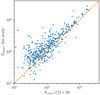 |
Fig. 1. Comparison between the number of stars in CAN+20 and in this study. The dashed line shows the identity relation. |
Figure 2 shows an example of the results of our clustering procedure on two well-known clusters, Blanco 1 and NGC 2682. In both cases, we recover almost all members identified by CAN+20 and we extend the memberships far beyond the cores and reach the limits of our search radius. For NGC 2682, we identify many halo stars and confirm previous findings of Carrera et al. (2019). In the case of Blanco 1, the tidal tail that was reported by Zhang et al. (2020) is also detected by our method, in addition to halo stars. We detect vast coronae around a significant number of clusters, similarly to Meingast et al. (2021), who performed a 3D analysis on ten prominent and nearby clusters. We detect similar structures in the five clusters we have in common. These coronae extend to the edge of our search radius, suggesting that they are even larger. We detected these coronae even for distant clusters such as NGC 2477, which is located at 1415 pc.
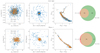 |
Fig. 2. Example of the results of our clustering procedure for NGC 2682 (upper panels) and Blanco 1 (lower panels). For each cluster, the three scatter plots represent (from left to right) a comparison between the members from CAN+20 (in orange) and ours (in blue) in proper motion space, in equatorial coordinate space, and in the color magnitude diagram. Rightmost panel: a Venn diagram for both clusters, in which the number of members in both studies is compared with members from CAN+20 in red, our members in green, and the overlap in orange. |
In order to test the hypothesis that the coronae can extend to very large distances from the core and that recovered members are limited by the search radii, we inspected the results of our method for the recently discovered OC COIN-Gaia 13 for different search radii. We queried the Gaia archive as described in Sect. 2.1, but we performed five concentric cone searches of increasing radius in steps of 20 pc. We show the resulting probability distributions and members recovered up to a radius of 150 pc in Fig. 3. We continuously identify members up to the edge of the cone search even at a radius of 150 pc. However, the number of members stopped increasing after a radius of 80 pc was reached, which we interpret as the limit of the corona. This also shows that for very extended fields, a probability cutoff of 0.5 might no longer be the best compromise.
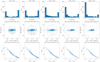 |
Fig. 3. Probability distribution (top row), distribution of the recovered members of COIN-Gaia 13 on the celestial sphere (middle row), and color magnitude diagram (bottom row) for a concentric search radius from 70 to 150 pc in steps of 20 pc. In each of the middle panels, we show the edge of the search radius in degrees with the dotted blue circle, and we indicated the number of stars that pass our probability cutoff. |
We computed the mean position and parallax of each OC by determining the maximum density point through a kernel density estimation. The mean proper motions were computed differently. The proper motion distributions are too flat to properly assume the maximum density point. Therefore we used the same method as CAN+20: we calculated the median value after removing outliers away from the median by more than three median absolute deviations (MAD). The mean astrometric parameters of our OC sample and the comparison to those of CAN+20 are presented in Fig. 4. The mean of the residuals of the comparison to CAN+20 is well centered on zero for the positions and proper motions. Inevitably, for some clusters, the members of CAN+20 and ours are different: either some members were not retrieved by HDBSCAN, or we have many more members now (which represent the majority of cases). This creates significant differences in the mean centers and proper motions of some clusters compared to CAN+20, especially for clusters that are sparsely populated. However, for parallaxes, the distribution of the residuals shows a negligible offset of −0.008 mas and an MAD of 0.015 mas, which shows that our values and those of CAN+20 agree.
 |
Fig. 4. Distribution of the residuals of the mean cluster parameters of CAN+20 and those calculated in this study. The solid orange line represents the mean of the distribution, and the dashed orange lines show the 1σ standard deviation from the mean. For clarity, the offset between the mean positions calculated here and the previously reported mean positions are only shown in the range (−0.5, 0.5) degrees, even though nine and five OCs lie beyond this limit for the right ascension and declination, respectively. |
3. Radial density profiles
We measured the structural parameters of the OCs in our sample based on our new lists of members extended to the outskirts of the clusters. The radial density profile (RDP) is a good indicator to study the extension of the spatial distribution of the clusters members. When it is obtained, the resulting density profile can be characterized by means of the fit of the widely used King empirical function (King 1962).
3.1. Fitting procedure
The King profile is widely used to fit the radial density profile of OCs, although it was first introduced to describe the surface density of globular clusters (King 1962). It is defined as
 (1)
(1)
where k is a scaling constant related to the central density, Rc is the core radius, Rt is the tidal radius, and n(R) is the surface density in stars per squared parsec. Following Küpper et al. (2010), we added a constant c to the original formula of King (1962), also in stars per squared parsec. We expect c to be close to zero because we considered the most reliable cluster members. This constant significantly improved the quality of the fits for many clusters. The core radius was defined as the radius for which the value of the density is equal to half the central density. At the tidal radius, the cluster becomes indistinguishable from the field (King 1962). In our case, the tidal radius is therefore the radius for which the density is equal to c.
The first step in order to fit a model such as the King profile to a cluster is to determine its radial density profile. To do this, we first needed to calculate the distance between the stars of each cluster and the cluster center. The cluster centers were computed as described in Sect. 2. Some of the clusters of our sample, such as Ruprecht 98, have high declinations, and the distribution of their members in the sky is therefore subject to strong projection effects. Some clusters, especially the most nearby ones, are also sensitive to projection effects due to the curvature of the celestial sphere. To avoid these biases, we projected the coordinates of each star on the plane of the sky, tangential to the celestial sphere at the coordinates of the clusters centers, as suggested by van de Ven et al. (2006) and Olivares et al. (2018). The projected coordinates are defined for each cluster star as
 (2)
(2)
where D is the heliocentric distance of the cluster computed by CAN+20 in pc, and αc and δc are the cluster mean right ascension and declination.
The radial distance R of each star to the center of the cluster is
 (3)
(3)
We divided the spatial distribution of the stars on these projected coordinates into concentric rings. We used ten bins of one parsec width for the inner parts of the clusters, and then we progressively increased the width of these rings. We computed the density, which is defined as the number of stars per square parsec in each ring.
We fit the King profile with a maximum likelihood (ML) estimator considering Poissonian uncertainties for each point. We used the Markov chain Monte Carlo (MCMC) sampler emcee (Foreman-Mackey et al. 2013) and initialized eight walkers (two per parameter). For each walker, we assigned 10 000 iterations to converge, and we discarded the first 2000 iterations to compute the posterior. As recommended, the convergence of the chains was systematically checked based on the integrated autocorrelation time (Goodman & Weare 2010). The results of our fitting procedure are shown as an example for the cluster NGC 752 in Fig. 5, where we found a core radius  pc and a tidal radius of
  . We applied this procedure to the 233 clusters in our sample that have more than 100 members. We chose this lower limit in order to have a sufficient number of stars in the circular rings.
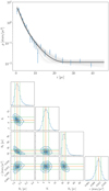 |
Fig. 5. Results of the King profile fit for the cluster NGC 752. Top panel: the blue dots are shown with Poissonian uncertainties. It also shows the best fit obtained with an ML estimator (solid black line), defined as the mode of the distributions of the parameters obtained through the 64 000 fits. The gray lines represent the uncertainties on the fits: we show 100 fits taken from the posterior distribution of the ML. Bottom panel: corresponding projection of the parameter posterior distribution. The orange lines show the mode of each distribution, and the dashed green line shows the 68% HDI. |
We only considered the fits for which no flag was raised by the integrated autocorrelation time regarding the convergence of the chains of the fitting procedure as satisfactory results. We also discarded the determinations of Rc with errors greater than 2.5 pc and the determinations of Rt with errors greater than 15 pc. This left estimates of Rc and Rt for 172 and 146 OCs, respectively. These two quality cuts are mostly useful to discard the cases for which the tidal radii are poorly constrained. Because of the sparse nature of OCs and, in some cases, of the contamination by field stars, the determination of the tidal radii is more challenging than the determination of the core radii (Oswalt & Gilmore 2013, p. 356).
3.2. Discussion
The tidal radius estimated in this study is a parameter of the King radial density profile and is not to be confused with the Jacobi radii introduced by (1987, p. 450). The Jacobi radius Rj is often referred to as the tidal radius, but is only a crude estimate of it. Unlike the tidal radius, the Jacobi radius does not require the density to be equal to zero at R = Rj.
The fitted cores and tidal radii for each cluster are shown as a function of their ages in Fig. 6. The core and tidal radii were computed as the mode of the parameter distributions of our ML procedure chains. The uncertainties represent the lower and upper bound of the 68% highest density interval (HDI) of the ML chains. The vast majority of clusters have a core radius between 1 and 2.5 pc, regardless of their age and number of members. The most frequent value of the core radius is ∼1.85 pc. The vast majority of the clusters with fewer than 250 members (in blue in the figure) have slightly lower values of Rc than the mode of the distribution, while more populated clusters tend to have higher values. Finally, the dispersion of the core radius decreases with increasing age of the clusters. This indicates that even if young clusters can have very concentrated cores, this feature is more common for old clusters. This agrees with the hypothesis discussed by Heggie & Hut (2003) that the evolution of the inner parts of the cluster is dominated by two-body relaxation, which causes the cluster core to shrink. Two-body relaxation is also known to cause mass segregation in clusters: massive stars are concentrated in the cores of the clusters, while less massive stars move in their outskirts. This might be connected to the observed decrease in core radius with age. As more massive stars are concentrated toward the cluster cores, the gravitational potential of the cores increases, which causes it to be denser. Mass segregation is studied in detail in Sect. 5. We point out that this decrease in the dispersion of the core radii might also be explained statistically: the clusters that deviate most from the mode of the distribution have the largest errors.
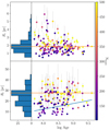 |
Fig. 6. Fitted core radii Rc (top) and tidal radii Rt (bottom) shown as a function of the logarithm of the cluster ages and their corresponding histograms. The color bar stands for the number of cluster members, and the mode of the distributions is overplotted with the solid orange line. A linear regression of the tidal radii vs age has been fitted with a least-squares method (blue line). |
The bottom panel of Fig. 6 shows that the distribution of the tidal radius is bimodal. It peaks around 28 pc, with a secondary peak at ∼18 pc. The majority of clusters with fewer than 250 members (in blue) have values of Rt ∼ 18 pc or lower, while almost all of the populated clusters (in yellow) have higher values. Additionally, the tidal radius increases mildly with cluster age. We illustrate this increase by overplotting a linear regression of the tidal radii versus the age of the clusters. To perform the fit, we used a simple least-squares method and took the uncertainties in the tidal radii into account. We obtained values of 4.64 ± 1.63 and −17.00 ± 13.87 for the slope and the y-intercept of the fit, respectively. This increase might again be connected to mass segregation or to cluster evaporation: because more stars have moved to the outskirts of the older clusters, they are more likely to be torn off from the clusters. Consequently, this might produce an increase in tidal radius with age.
Core and tidal radii of OCs have often been determined in the past by fitting a King profile. The most extensive catalog of radii was published before the launch of the Gaia mission by Kharchenko et al. (2013). Also before Gaia, Piskunov et al. (2007) published a catalog of radii for 236 OCs out of the 650 clusters with reliable memberships from the catalog ASCC-2.5. More recently, Angelo et al. (2021) studied the structural parameters of 38 OCs with Gaia DR2 data in detail. The comparison of our determinations of core and tidal radii with these three studies is shown in Fig. 7. We note that Angelo et al. (2021) searched for members at a maximum radius of 1° around the cluster centers computed by Dias et al. (2002). For most of their clusters, this is equivalent to a radius smaller than 30 pc. We therefore have very different member lists, which makes a close comparison difficult. Nevertheless, we can compare the distributions of Rc and Rt. As shown in Fig. 7, the similarity between the distribution of Rc in all the studies is striking, while the tidal radii computed here are much larger than those computed in the other studies. This is a direct consequence of our choice to search for members at larger distances from the center of each cluster compared to the previous studies. On the other hand, in the case of M 67/NGC 2682, Carrera et al. (2019) searched for members up to 150 pc around the center of the cluster. They fit a King function to the radial density profile and estimated a tidal radius of 80 pc, while we find a value of  pc. This suggests, as previously reported by Olivares et al. (2018), that the determination of the tidal radius is highly dependent on the size of the survey. Therefore our distribution of tidal radii is likely truncated because our queries around each cluster was limited to 50 pc.
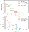 |
Fig. 7. Distribution of the core (top) and tidal (bottom) radii computed in this study and by Piskunov et al. (2007), Kharchenko et al. (2013), and Angelo et al. (2021). |
Because we considered only cluster members in our fitting procedure, the c constant from Eq. (1) (which is equivalent to a field constant density) should be close to 0. When it is higher, it gives us an estimate of the number of contaminants for each cluster. The median proportion of contamination in our sample is ∼13%. This estimation of the contamination rate is biased for some clusters and leads to a high contamination rate. As explained in Sect. 2.3, our distribution of members is likely truncated for populated clusters. This leads to an underestimation of the tidal radius of these clusters with typical values of ∼30 pc. The members that are detected beyond this estimation of the tidal radius act as a background field density in the fit, leading to an overestimation of the c constant, that is, of the contamination rate. Moreover, the King profile might not be the best way to describe the density of some clusters with extended halos (Küpper et al. 2010), especially if they are elongated, like for Blanco 1: tidal-tail stars also act as a background field density here. We therefore fit a GMM on the spatial distribution of members (see Sect. 4).
Schilbach et al. (2006) noted an increase in the size of the clusters with altitude above the Galactic plane and that this increase was especially significant for clusters older than ∼22 Myr. They also reported that large clusters were found at large Galactocentric distances. They concluded that clusters located within the solar orbit whose orbit is inclined low with respect to the Galactic plane are likely to be rapidly dissolved by encounters with giant molecular clouds or by Galactic tidal stripping. In contrast, clusters whose orbit lies outside the solar orbit and that reach high altitudes are more likely to survive longer and to avoid being stripped of their members. None of these correlations are found by us, even when we divide our sample of OCs into different age bins. We therefore cannot confirm these findings. More recently, Dib et al. (2018) also failed to confirm these findings.
4. Gaussian mixture models
The function described in the previous section assumes a circular distribution of the members. In order to study the morphology of the OCs without this assumption, we fit a GMM on the spatial distribution of members of each OC. A GMM is a probabilistic model assuming that the data can be described by a combination of a finite number of Gaussian distributions.
4.1. Fitting procedure
To remove projection effets due to clusters located at high Galactic latitudes and to members located far from the cluster centers, we used Eq. (2) to project the Galactic latitude and longitude of each star in a cluster on a plane tangential to the celestial sphere. In order to fit a GMM on these coordinates, we used a variational GMM with a Dirichlet process prior3. This algorithm is a variant of the classical GMM and allows inferring the effective number of components from the data. Usually, classical GMM fitting takes advantage of the expectation maximization (EM) algorithm. In the EM algorithm, the parameters of the Gaussians are randomly initialized (the user can also provide a first guess), and the algorithm computes the probability with which each data point belongs to each component. The parameters of each Gaussian are tuned in order to maximize the likelihood of the data under this model. Tuning the parameters of each Gaussian over a sufficient number N of iterations always allows converging to a local maximum of the likelihood. The variational inference extends the EM approach by adding information through a prior distribution: the Dirichlet process. With the Dirichlet process prior, the number of components set by the user is only used as an upper bound. The algorithm automatically draws the number of components from the data, activates a component and attributes stars to this component only if necessary: if the maximum number of components is set to 3 but the Dirichlet process only detects 2, it sets the relative weight of one of the component to ∼0.
As explained in Sect. 2, we realized through visual inspection that some clusters were elongated in their outskirts, which could correspond to a tidal tail. For a fraction of these OCs, the number of members is between 50 and 100. In order to characterize as many tidal tails as possible, we fit a GMM on all the clusters with more than 50 members. We also note that most of the clusters present a prominent core and an extended halo. Consequently, we systematically tried to fit three components to the sky distribution of the members of each cluster. One component would correspond to the core of the cluster, the second component to the eventual tidal tail, and the third component to the cluster halo or coronae. Because not all the clusters show a tidal tail, the Dirichlet process is therefore well suited for our purpose: if only two components are detected, the weight of the component standing for the tidal tail is supposed to be close to zero.
Since there is a stochastic initialisation in the variational inference algorithm, the fit does not always converge on the same solution. Therefore, in order to estimate the parameters of the Gaussians better, we ran the fitting algorithm for each cluster one thousand times. The parameters of the resulting Gaussians were then chosen as the mode of the resulting distributions, and their standard errors were computed as  with Niter = 1000. In addition, we noted the fits were better when the algorithm forced the Gaussians to be concentric.
For some clusters, the algorithm found a prominent and elongated component of the GMM that might be associated with a tidal tail. However, we were unable to find a clear cut in weights or eccentricity based on which clusters with and without elongation might be separated. The reason is the large variety of clusters and environments we studied. In particular, the most populated clusters (more than 500 members) with a dense core always had a second component with a significant weight, even if it does not represent a tidal tail, but more likely the outskirts of the core. In most of these cases, the results with two components were sufficient to fit the distribution. We also tried to separate the clusters with and without a tidal tail using the length of the semi-major axis of the second component, the number of stars attributed to each component, or the ratio of the semi-minor and semi-major axis of the second component. However, we did not find an ideal way to separate the two subsamples with accuracy and therefore identified them visually. We defined a subsample of 71 OCs with this feature. We show the results for four clusters that are remarkably elongated in Fig. 8. A prominent halo is also noticeable around the cores of the four clusters. The legend in each panel of Fig. 8 shows the weights attributed to each component by the algorithm.
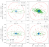 |
Fig. 8. Example of four clusters for which we detect a tidal tail. The blue, green, and red ellipses represent the 3 σ ellipse fit on the distribution of the stars standing for the core, the tidal tail, and the halo, respectively. The stars are colored according to which components they most likely belong. The relative weights of each component are indicated in each panel. |
For the 71 clusters that were identified as having a tidal tail, we study the parameters of the three-component solution below. For the remaining clusters, we adopt the parameters of the two-component solution.
Hu et al. (2021) used a similar approach and fit a two-component model using a least-squares ellipse fitting on 265 OCs from the membership catalog by Cantat-Gaudin et al. (2018b). A direct and systematic comparison of their results and ours is not possible because they investigated much smaller areas around each cluster than we did. However, we checked some clusters individually. For instance, we find a tidal tail around NGC 752 (Fig. 8) with roughly the same orientation and eccentricity as they did, according to their Fig. 1. We found an orientation of 6.146 degrees with the Galactic plane and an ellipticity of 0.776 ± 0.002, while they found an angle of 4.697 degrees and an ellipticity of 0.615 ± 0.342.
4.2. Discussion
The majority of the clusters has a significant corona. Among the clusters that are well described by a two-component solution, 254 have a weight higher than 0.1 attributed to the corona. In Fig. 9 we show the weights of the halo as a function of the age for these clusters. Even if young clusters can have halos with very various weights, we did not find any old clusters with a halo with a weight higher than 0.4. This indicates that as clusters grow old, fewer stars are part of the corona, and a higher proportion of their stars tend to be concentrated in the cluster cores. This process might be connected to the mass segregation and the cluster evaporation. Mass segregation tends to cause the most massive stars of a cluster to sink into its center and the less massive stars to move toward its outskirts. On the other hand, if the cluster progressively evaporates, the outskirt stars are eventually torn out off the corona and thus reduce its weight, as is shown in Fig. 9.
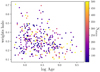 |
Fig. 9. Distribution of the weights of the second Gaussian component (associated with a halo structure) as a function of the age for the subsample of clusters that is best fit with a two-component model. |
Hu et al. (2021) and Zhai et al. (2017) also fit ellipses on the distribution of members projected on the plane of the sky. They noted an increase in the ellipticity of the outer parts with age in a sample of 265 and 154 clusters, respectively. Based on 31 OCs, Chen et al. (2004) also noted an increase in the circularity of the inner parts of OCs with age, especially at high altitudes. They attributed this process to the internal dynamical relaxation process in OCs. Internal dynamics can shape clusters cores after ∼100 Myr, while younger clusters inherit their shape from the initial conditions of the cluster formation. We considered the fitted parameters of the core and halo ellipses: the length of the semi-major axis, the eccentricity, and the orientation. We searched for correlations with Galactocentric radius, age, and number of stars, but found no relevant trend.
As mentioned in Sect. 4.1, we detected 71 tidal tails. We show the distribution of the axis ratio of each fitted component for our whole sample of clusters in Fig. 10. In the top panel, we show the distribution of the axis ratio of the cores. It shows that the vast majority of the clusters have a nearly circular core as the distribution peaks between 0.8 and 0.9. We examined the clusters with the most elliptical shape. They do not contain many stars in their center, which makes their ellipticity less reliable. In the middle panel we show the distribution of the axis ratio of the tidal tails. They are all very elongated, and the axis ratio of ∼70% of the identified tidal tails is lower than 0.3. Finally, the bottom panel shows the distribution of the axis ratio of the corona. In most of the cases, the corona is almost circular, and in the few cases in which the ratio of the axis is lower than 0.5, the number of stars in the halo is again very low.
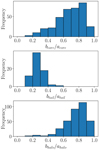 |
Fig. 10. Distribution of the axis ratio of each component. |
We can characterize the components of the 71 clusters in our sample that show a tidal tail by considering the properties of their components. We show the length of the core semi-major axis as a function of cluster age and of the logarithm of the number of stars belonging to it in Fig. 11. The top panel shows that the clusters with tidal tails also follow the decreasing relation of the core radii with age found in Fig. 6 for all clusters. In the lower panel, the length of the axis also has a decreasing dependence with the number of stars belonging to it. This means that even if populated clusters might be thought to have larger cores, their stronger gravitational binding, in contrast, make them much denser OCs. We searched in vain for correlations of tidal tail and halo semi-major axis lengths, eccentricities, and orientations with cluster age or with their locations in the Galaxy.
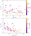 |
Fig. 11. Length of the semi-major axis of the core of our clusters with age (top) and with the logarithm of the number of stars belonging to it (bottom) for the subsample of clusters with a tidal tail. Top panel: the color bar stands for the total number of stars belonging to the cluster, and in the bottom panel, it represents the relative weights of the core. |
Sixteen tidal tails have already been characterized in the literature. Eight of them are part of our sample: Coma Berenices, Ruprecht 147, Praesepe, Blanco 1, NGC 752, NGC 7092, NGC 2516, and Platais 9. Our study identifies tidal tails for Coma Berenices, Blanco 1, NGC 752, NGC 7092, and NGC 2516, which were previously found by Tang et al. (2019), Zhang et al. (2020), Bhattacharya et al. (2021), and Meingast et al. (2021), respectively. We found the same orientations as these authors. The tidal tails of Ruprecht 147, Praesepe, and Platais 9 were characterized by Yeh et al. (2019), Röser & Schilbach (2019), Gao (2020), and Meingast et al. (2021), respectively, who found them to be roughly aligned with the line of sight. We cannot detect such tidal tails owing to our 2D analysis of the distribution of stars projected on the sky.
Meingast et al. (2021) identified extended stellar populations similar to the tidal structure in 9 out of 10 OCs. They attributed these structures to the imprint of the parent molecular cloud relic structure for clusters younger than 50 Myr and to stripped cluster stars for clusters older than 100 Myr. Pang et al. (2021) also found elongated shapes in 8 of their 13 OCs sample in the form of filament-like substructures, reminiscent of the star formation history of the cluster for clusters younger than 50 Myr and to tidal stripping for the oldest clusters (NGC 2516, Blanco 1, Coma Berenices, NGC 6633, and Ruprecht 147). We find the same structures for the clusters we have in common (with the exception of Ruprecht 147). According to Lada & Lada (2003), Bonnell & Davies (1998), and Bastian et al. (2009), in only a few million years, a cluster would reach a state of equilibrium and remove the star distribution that it inherited from the star formation process. As no clusters younger than 50 Myr are included in our sample, the vast majority of the tidal tails in our sample can be attributed to dynamical effects and to tidal stripping.
5. Mass segregation
According to the standard view, mass segregation in OCs is believed to increase with age (Kroupa 1995; Dib et al. 2018). Old clusters are therefore thought to be more frequently mass segregated than young clusters. Our membership analysis over extended regions of OCs of various age means that we can verify or refute this hypothesis.
5.1. Method
In order to measure the degree of mass segregation, we applied the method proposed by Allison et al. (2009a) that is widely used to quantify and detect mass segregation in stellar clusters (Nony et al. 2021; Dib et al. 2018; Plunkett et al. 2018; Román-Zúñiga et al. 2019). This method works by comparing the length of the minimum spanning tree (MST) of the most massive stars of a cluster with the length of the MST of a set of the same number of randomly chosen stars. An MST of a set of points is the path connecting all the points, with the shortest possible path length and without any closed loops. In a given set of points, only one MST can be drawn. We computed the MST by using the csgraph routine implemented in the scipy python module (Virtanen et al. 2020). In all the cases, we drew the MST in the same set of coordinates as defined in Eq. (2). The mass-segregation ratio (MSR) ΛMSR is then defined as follows:
 (4)
(4)
with ⟨lrandom⟩ being the average length of the MST of N randomly chosen stars and lmassive the length of the MST of the N most massive stars. The average length ⟨lrandom⟩ was calculated over 100 iterations, where at each iteration, we drew a different subsample of random stars allowing us to simultaneously calculate σrandom, the standard deviation of the length of the MST of these N stars. We used the G magnitude of the stars as a proxy for the mass. The MSR ΛMSR was always calculated for a subset of N stars. A result of ΛMSR greater than 1 means that the N most massive stars are more concentrated than a random sample and therefore that the cluster shows signs of mass segregation. We conducted this analysis for all the clusters containing more than 50 stars. In each cluster, we calculated the MSR starting at N = 5 up to the number of cluster members. We started at N = 5 because for lower N, the value is not statistically significant. For clusters with more than 100 stars, we stopped at N = 100 because the MSR only shows a gradual decrease to reach unity.
Figure 12 shows the MSR for the cluster Collinder 394 for increasing values of N. There are several degrees of mass segregation. First the 20 most massive stars have a value for ΛMSR ∼ 3.2. Then ΛMSR drops, with a plateau for 20 < N < 26 at a value of ∼1.7. The MSR then drops to 1.4 and progressively decreases. This analysis tells us that in Collinder 394, the 20 most massive stars are 3.2 times closer to each other than the typical separation of 20 random stars in the cluster, and that the 25 most massive stars of cluster are 70% more concentrated than any set of 25 members. After this, the remaining stars progressively approach ΛMSR ∼ 1.
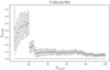 |
Fig. 12. Mass segregation ratio ΛMSR(N) for the cluster Collinder 394 as a function of the number of stars used to draw the MST. The dotted blue line shows the limit ΛMSR = 1 after which stars do not show signs of mass segregation. |
5.2. Discussion
Maschberger et al. (2010) studied the very early stages of clusters through N-body simulations and noted that the ten most massive stars of a cluster quickly formed a very concentrated system after the clusters formed. We represent in Fig. 13 the distribution of the MSR of the tenth most massive stars (Λ10) as a function of their parent cluster ages, Galactocentric radii, and altitude above (or below) the Galactic plane. No particular trend regarding the evolution of mass segregation with these parameters is visible, even though we would expect an increase in the mass segregation with age (Dib et al. 2018). For consistency, we also checked if some trend appeared in the MSR of the fifth to the twentieth most massive stars, but this was not conclusive.
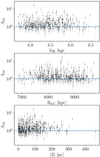 |
Fig. 13. Mass segregation ratio Λ10 of the ten most massive stars of each cluster as a function of OC ages (top), Galactocentric radii (middle), and absolute value of the altitude above the Galactic midplane (bottom). The dotted blue line shows the limit ΛMSR = 1. |
The lack of a net relation between Λ10 with age might be explained by the fact that OCs formed with very different levels of mass segregation (Dib et al. 2018). For instance, the very young cluster Trapezium, the core of the Orion Nebula Cluster, shows evidence of mass segregation even though its age is ∼1 Myr (Bonnell & Davies 1998; Allison et al. 2009a). This was referred to as primordial mass segregation (de Grijs et al. 2003). Mass segregation in young clusters was first thought to be caused by the initial conditions of the cluster formation, but recent N-body simulations suggested that mass segregation occurs on timescales of about a few million years. This implies that clusters younger than their dynamical relaxation time can show signs of mass segregation. This could be due to dynamical interactions through the merging of smaller substructures. In this scenario, clusters are born with a significant number of clumps. Each of these small clumps can then mass segregate on short timescales through dynamical interactions. The merging of these multiple clumps later gives birth to a cluster that inherited the substructure segregation (McMillan et al. 2007; Allison et al. 2009b, 2010; Maschberger et al. 2010). This gives a more complex view of what is expected to be observed in our sample of OCs.
In order to investigate the age dependence of the mass segregation in a different way, we measured the proportion of stars per cluster that has ΛMSR > 2. We defined two subsamples: one in which more than 10% of the stars have ΛMSR > 2, and the other one being the complementary subsample. For example, Fig. 12 shows that in Collinder 394, the MSR for 20 stars is higher than 2. As it counts 703 members, only 2% of Collinder 394 stars have ΛMSR > 2, and Collinder 394 is therefore part of the complementary subsample where fewer than 10% of the clusters members are highly mass segregated. The age distribution of these two subsamples is shown in Fig. 14. Even if no trend between Λ10 and the cluster ages was noticeable in Fig. 13, it is clear here that OCs with a large proportion of stars that are strongly mass segregated are older on average than the clusters with few highly mass-segregated stars.
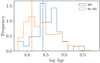 |
Fig. 14. Age distribution of two subsamples of OCs: one sample in which more than 10% of the stars have ΛMSR > 2 (in blue), and one sample in which fewer than 10% of the stars have ΛMSR > 2 (in orange). The vertical dotted line shows the mode of each distribution. |
This might be related with the signs of evaporation observed in Sect. 4. In Fig. 9, we noted that old clusters have fewer stars in their halo on average than young clusters. As old clusters are proportionally more mass segregated than young clusters, low-mass stars should be pushed to the outskirts of the clusters, which increases the relative weights of the halo. As we observe the opposite, this might indicate that cluster evaporation process is more efficient than mass segregation.
6. Conclusion
We developed a method that can identify members in the peripheral area of OCs up to 50 pc from their center. The method is based on the unsupervised clustering algorithm HDBSCAN, which can detect overdensities in the astrometric space (μα*, μδ, ϖ) even in datasets with varying density. We applied this method on 467 OCs from CAN+20 that are located closer than 1.5 kpc and are older than 50 Myr. We report memberships for 389 OCs. The 78 remaining clusters are too embedded in their field for our method to properly distinguish them from their neighbors. For the vast majority of clusters, we identify many more members than were known previously. For COIN-Gaia 13, a very extended cluster, we tried to increase our search radius and recovered members up to 150 pc from the cluster centers. This highlights that studies focused on small samples of clusters should search for members even at large distances from the cluster centers, as reported by Meingast et al. (2021) or Carrera et al. (2019).
We identified vast coronae around almost all the clusters, which in most cases reach the maximum radius of the investigated area. We also identified tidal tails for ∼71 OCs. Previous detections of coronae or tidal tails of OCs were focused on smaller samples of nearby clusters. Since we worked with the 2D projected distribution of stars, we were able to perform a systematic study of OCs at large heliocentric distances, and we multiplied the number of identified clusters with a tidal tail by more than four.
The primary goal of this paper was to determine the structural parameters of the clusters for which we obtained new members at a large radius. To do this, we fit the radial density profile of each cluster with more than 100 members with a King function in order to study their core and tidal radii. We find similar core radii to those published in previous studies, but as we find members at a much larger radius than in previous studies, we also find much larger tidal radii. The distribution of the fitted core radii shows a concentration between 1 and 2.5 pc, regardless of the age or number of cluster members. Older clusters tend to have smaller Rc than young clusters. The values converge toward 1.85 pc at an age of 1 Gyr. The tidal radii peak at about 30 pc, but more importantly, they seem to increase with age in what might be a sign of mass segregation, dissolution, or a combination of both processes. The tidal radius distribution might be biased due to the limit of 50 pc that we used to query the Gaia EDR3 catalog. A fraction of the investigated clusters may extend to larger radii than this, as shown in Sect. 2.3 with the example of COIN-Gaia 13.
We fit GMMs on the spatial distribution of members projected on a plane perpendicular to the celestial sphere. This is particularly suitable for the clusters for which we detected an elongated tidal tail, as the King function previously used assumes a spherical distribution of members. We used a three-component GMM on the 71 clusters with a tidal tail in which one component represented the core of the cluster, one the tidal tail, and one the corona. For the other clusters, we adopted a two-component GMM with a core and a halo. We searched for correlations between the parameters of the fitted Gaussians with the characteristics of the clusters (i.e. their age, location, and number of members). Old clusters in the 71 clusters of our sample with a tidal tail are more prone to have small cores than young clusters. The relative weight of the corona of old clusters was lower than for young clusters on average. This implies that with an increasing age, the proportion of stars in the cluster halos decreases, either because stars move to the center of the cluster or because outer stars are ejected from the cluster.
We applied the method proposed by Allison et al. (2009a) to measure the degree of mass segregation of our sample of OCs. We found no trend of the MSR, measured through the ten most massive stars, with age, Galactocentric distance, or with the altitude of the cluster above the Galactic midplane. However, clusters with significant number of stars with a strong MSR are older on average than clusters with a few stars that are strongly mass segregated. Coupled with a lower proportion of stars populating the clusters halos, this highlights the fact that the various physical processes in the disruption of clusters act on shorter timescales than mass segregation.
We did not use the sky coordinates to compute our membership lists like Castro-Ginard et al. (2018, 2019; 2020) because we study the halos of known clusters.
This enables adopting a different threshold that is more specific to other scientific objectives.
Algorithm implemented in the scikit-learn python package (Pedregosa et al. 2011).
Acknowledgments
This work has made use of data from the European Space Agency (ESA) mission Gaia (http://www.cosmos.esa.int/Gaia), processed by the Gaia Data Processing and Analysis Consortium (DPAC, https://www.cosmos.esa.int/web/Gaia/dpac/consortium). We acknowledge the Gaia Project Scientist Support Team and the Gaia DPAC. Funding for the DPAC has been provided by national institutions, in particular the institutions participating in the Gaia Multilateral Agreement. This research made extensive use of the SIMBAD database, and the VizieR catalog access tool, operated at the CDS, Strasbourg, France, and of NASA Astrophysics Data System Bibliographic Services. This research has made use of Astropy (Astropy Collaboration 2013), Topcat (Taylor 2005). Y.T., C.S., and L.C. acknowledge support from “programme national de physique stellaire” (PNPS) and from the “programme national cosmologie et galaxies” (PNCG) of CNRS/INSU. L.C. acknowledges the support of the postdoc fellowship from French Centre National d’Etudes Spatiales (CNES). This work was (partially) supported by the Spanish Ministry of Science, Innovation and University (MICIU/FEDER, UE) through grant RTI2018-095076-B-C21, and the Institute of Cosmos Sciences University of Barcelona (ICCUB, Unidad de Excelencia ‘María de Maeztu’) through grant CEX2019-000918-M. J.O. acknowledges financial support from: (i) from the European Research Council (ERC) under the European Union’s Horizon 2020 research and innovation program (grant agreement No 682903, P.I. H. Bouy), (ii) the French State in the framework of the “Investments for the future” Program, IdEx Bordeaux, reference ANR-10-IDEX-03-02, and iii) the Agencia Estatal de Investigación of the Ministerio de Ciencia, Innovación y Universidades through project PID2019-109522GB-C53.
References
- Allison, R. J., Goodwin, S. P., Parker, R. J., et al. 2009a, MNRAS, 395, 1449 [Google Scholar]
- Allison, R. J., Goodwin, S. P., Parker, R. J., et al. 2009b, ApJ, 700, L99 [Google Scholar]
- Allison, R. J., Goodwin, S. P., Parker, R. J., Portegies Zwart, S. F., & de Grijs, R. 2010, MNRAS, 407, 1098 [NASA ADS] [CrossRef] [Google Scholar]
- Alves, J., Zucker, C., Goodman, A. A., et al. 2020, Nature, 578, 237 [NASA ADS] [CrossRef] [Google Scholar]
- Angelo, M. S., Corradi, W. J. B., Santos, J. F. C., Maia, F. F. S., & Ferreira, F. A. 2021, MNRAS, 500, 4338 [Google Scholar]
- Artyukhina, N. M., & Kholopov, P. N. 1964, Sov. Astron., 7, 840 [Google Scholar]
- Astropy Collaboration (Robitaille, T. P., et al.) 2013, A&A, 558, A33 [NASA ADS] [CrossRef] [EDP Sciences] [Google Scholar]
- Bailer-Jones, C. A. L. 2015, PASP, 127, 994 [Google Scholar]
- Bastian, N., Gieles, M., Ercolano, B., & Gutermuth, R. 2009, MNRAS, 392, 868 [NASA ADS] [CrossRef] [Google Scholar]
- Baumgardt, H., & Kroupa, P. 2007, MNRAS, 380, 1589 [NASA ADS] [CrossRef] [Google Scholar]
- Bhattacharya, S., Agarwal, M., Rao, K. K., & Vaidya, K. 2021, MNRAS, 505, 1607 [NASA ADS] [CrossRef] [Google Scholar]
- Binney, J., & Tremaine, S. 1987, Galactic Dynamics (Princeton, N.J. : Princeton University Press) [Google Scholar]
- Bonnell, I. A., & Davies, M. B. 1998, MNRAS, 295, 691 [CrossRef] [Google Scholar]
- Campello, R. J. G. B., Moulavi, D., & Sander, J. 2013, in Advances in Knowledge Discovery and Data Mining, eds. J. Pei, V. S. Tseng, L. Cao, H. Motoda, & G. Xu (Berlin, Heidelberg: Springer), 160 [Google Scholar]
- Cantat-Gaudin, T., Jordi, C., Vallenari, A., et al. 2018a, A&A, 618, A93 [NASA ADS] [CrossRef] [EDP Sciences] [Google Scholar]
- Cantat-Gaudin, T., Vallenari, A., Sordo, R., et al. 2018b, A&A, 615, A49 [NASA ADS] [CrossRef] [EDP Sciences] [Google Scholar]
- Cantat-Gaudin, T., Anders, F., Castro-Ginard, A., et al. 2020, A&A, 640, A1 [NASA ADS] [CrossRef] [EDP Sciences] [Google Scholar]
- Carrera, R., Pasquato, M., Vallenari, A., et al. 2019, A&A, 627, A119 [NASA ADS] [CrossRef] [EDP Sciences] [Google Scholar]
- Castro-Ginard, A., Jordi, C., Luri, X., et al. 2018, A&A, 618, A59 [NASA ADS] [CrossRef] [EDP Sciences] [Google Scholar]
- Castro-Ginard, A., Jordi, C., Luri, X., Cantat-Gaudin, T., & Balaguer-Núñez, L. 2019, A&A, 627, A35 [NASA ADS] [CrossRef] [EDP Sciences] [Google Scholar]
- Castro-Ginard, A., Jordi, C., Luri, X., et al. 2020, A&A, 635, A45 [NASA ADS] [CrossRef] [EDP Sciences] [Google Scholar]
- Chen, W. P., Chen, C. W., & Shu, C. G. 2004, AJ, 128, 2306 [NASA ADS] [CrossRef] [Google Scholar]
- de Grijs, R., Gilmore, G. F., & Johnson, R. 2003, in New Horizons in Globular Cluster Astronomy, eds. G. Piotto, G. Meylan, S. G. Djorgovski, & M. Riello, ASP Conf. Ser., 296, 207 [NASA ADS] [Google Scholar]
- de La Fuente Marcos, R. 1996, A&A, 314, 453 [NASA ADS] [Google Scholar]
- Dias, W. S., Alessi, B. S., Moitinho, A., & Lépine, J. R. D. 2002, A&A, 389, 871 [NASA ADS] [CrossRef] [EDP Sciences] [Google Scholar]
- Dib, S., Schmeja, S., & Parker, R. J. 2018, MNRAS, 473, 849 [Google Scholar]
- Dinnbier, F., & Kroupa, P. 2020a, A&A, 640, A84 [EDP Sciences] [Google Scholar]
- Dinnbier, F., & Kroupa, P. 2020b, A&A, 640, A85 [EDP Sciences] [Google Scholar]
- Ester, M., Kriegel, H. P., Sander, J., & Xu, X. 1996, in Proceedings of the Second International Conference on Knowledge Discovery and Data Mining, KDD’96 (AAAI Press), 226 [Google Scholar]
- Fabricius, C., Luri, X., Arenou, F., et al. 2021, A&A, 649, A5 [NASA ADS] [CrossRef] [EDP Sciences] [Google Scholar]
- Foreman-Mackey, D., Hogg, D. W., Lang, D., & Goodman, J. 2013, PASP, 125, 306 [Google Scholar]
- Gaia Collaboration (Brown, A. G. A., et al.) 2018, A&A, 616, A1 [NASA ADS] [CrossRef] [EDP Sciences] [Google Scholar]
- Gaia Collaboration (Brown, A. G. A., et al.) 2020, A&A, 649, A1 [Google Scholar]
- Gao, X. 2020, ApJ, 894, 48 [NASA ADS] [CrossRef] [Google Scholar]
- Goodman, J., & Weare, J. 2010, Commun. Appl. Math. Comput. Sci., 5, 65 [Google Scholar]
- Grice, N. A., & Dawson, D. W. 1990, PASP, 102, 881 [NASA ADS] [CrossRef] [Google Scholar]
- Heggie, D., & Hut, P. 2003, The Gravitational Million-Body Problem: A Multidisciplinary Approach to Star Cluster Dynamics [Google Scholar]
- Hillenbrand, L. A., & Hartmann, L. W. 1998, ApJ, 492, 540 [NASA ADS] [CrossRef] [Google Scholar]
- Hu, Q., Zhang, Y., Esamdin, A., Liu, J., & Zeng, X. 2021, ApJ, 912, 5 [NASA ADS] [CrossRef] [Google Scholar]
- Hunt, E. L., & Reffert, S. 2021, A&A, 646, A104 [NASA ADS] [CrossRef] [EDP Sciences] [Google Scholar]
- Jerabkova, T., Boffin, H. M. J., Beccari, G., et al. 2021, A&A, 647, A137 [NASA ADS] [CrossRef] [EDP Sciences] [Google Scholar]
- Kharchenko, N. V., Piskunov, A. E., Schilbach, E., Röser, S., & Scholz, R. D. 2013, A&A, 558, A53 [NASA ADS] [CrossRef] [EDP Sciences] [Google Scholar]
- King, I. 1962, AJ, 67, 471 [Google Scholar]
- Kounkel, M., & Covey, K. 2019, AJ, 158, 122 [Google Scholar]
- Krone-Martins, A., & Moitinho, A. 2014, A&A, 561, A57 [NASA ADS] [CrossRef] [EDP Sciences] [Google Scholar]
- Kroupa, P. 1995, MNRAS, 277, 1522 [NASA ADS] [CrossRef] [Google Scholar]
- Krumholz, M. R., McKee, C. F., & Bland-Hawthorn, J. 2019, ARA&A, 57, 227 [NASA ADS] [CrossRef] [Google Scholar]
- Küpper, A. H. W., MacLeod, A., & Heggie, D. C. 2008, MNRAS, 387, 1248 [Google Scholar]
- Küpper, A. H. W., Kroupa, P., Baumgardt, H., & Heggie, D. C. 2010, MNRAS, 407, 2241 [NASA ADS] [CrossRef] [Google Scholar]
- Lada, C. J., & Lada, E. A. 2003, ARA&A, 41, 57 [Google Scholar]
- Lamers, H. J. G. L. M., & Gieles, M. 2006, A&A, 455, L17 [NASA ADS] [CrossRef] [EDP Sciences] [Google Scholar]
- Lindegren, L., Bastian, U., Biermann, M., et al. 2021, A&A, 649, A4 [EDP Sciences] [Google Scholar]
- Liu, L., & Pang, X. 2019, ApJS, 245, 32 [NASA ADS] [CrossRef] [Google Scholar]
- Maschberger, T., Clarke, C. J., Bonnell, I. A., & Kroupa, P. 2010, MNRAS, 404, 1061 [NASA ADS] [CrossRef] [Google Scholar]
- Mathieu, R. D. 1984, ApJ, 284, 643 [NASA ADS] [CrossRef] [Google Scholar]
- McInnes, L., Healy, J., & Astels, S. 2017, J. Open Source Softw., 2, 205 [NASA ADS] [CrossRef] [Google Scholar]
- McMillan, S. L. W., Vesperini, E., & Portegies Zwart, S. F. 2007, ApJ, 655, L45 [Google Scholar]
- Meingast, S., & Alves, J. 2019, A&A, 621, L3 [NASA ADS] [CrossRef] [EDP Sciences] [Google Scholar]
- Meingast, S., Alves, J., & Rottensteiner, A. 2021, A&A, 645, A84 [NASA ADS] [CrossRef] [EDP Sciences] [Google Scholar]
- Nilakshi, S. R., Pandey, A. K., & Mohan, V. 2002, A&A, 383, 153 [NASA ADS] [CrossRef] [EDP Sciences] [Google Scholar]
- Nony, T., Robitaille, J. F., Motte, F., et al. 2021, A&A, 645, A94 [NASA ADS] [CrossRef] [EDP Sciences] [Google Scholar]
- Olivares, J., Moraux, E., Sarro, L. M., et al. 2018, A&A, 612, A70 [NASA ADS] [CrossRef] [EDP Sciences] [Google Scholar]
- Oswalt, T. D., & Gilmore, G. 2013, Planets, Stars and Stellar Systems, 5 [Google Scholar]
- Pang, X., Li, Y., Yu, Z., et al. 2021, ApJ, 912, 162 [NASA ADS] [CrossRef] [Google Scholar]
- Pedregosa, F., Varoquaux, G., Gramfort, A., et al. 2011, J. Mach. Learn. Res., 12, 2825 [Google Scholar]
- Piecka, M., & Paunzen, E. 2021, BAJ, submitted [arxiv:2107.07230v1] [Google Scholar]
- Piskunov, A. E., Schilbach, E., Kharchenko, N. V., Röser, S., & Scholz, R. D. 2007, A&A, 468, 151 [NASA ADS] [CrossRef] [EDP Sciences] [Google Scholar]
- Plunkett, A. L., Fernández-López, M., Arce, H. G., et al. 2018, A&A, 615, A9 [NASA ADS] [CrossRef] [EDP Sciences] [Google Scholar]
- Román-Zúñiga, C. G., Alfaro, E., Palau, A., et al. 2019, MNRAS, 489, 4429 [Google Scholar]
- Röser, S., & Schilbach, E. 2019, A&A, 627, A4 [NASA ADS] [CrossRef] [EDP Sciences] [Google Scholar]
- Röser, S., Schilbach, E., & Goldman, B. 2019, A&A, 621, L2 [NASA ADS] [CrossRef] [EDP Sciences] [Google Scholar]
- Schilbach, E., Kharchenko, N. V., Piskunov, A. E., Röser, S., & Scholz, R. D. 2006, A&A, 456, 523 [NASA ADS] [CrossRef] [EDP Sciences] [Google Scholar]
- Sim, G., Lee, S. H., Ann, H. B., & Kim, S. 2019, J. Korean Astron. Soc., 52, 145 [NASA ADS] [Google Scholar]
- Tang, S.-Y., Pang, X., Yuan, Z., et al. 2019, ApJ, 877, 12 [Google Scholar]
- Taylor, M. B. 2005, in Astronomical Data Analysis Software and Systems XIV, eds. P. Shopbell, M. Britton, & R. Ebert, ASP Conf. Ser., 347, 29 [Google Scholar]
- van de Ven, G., van den Bosch, R. C. E., Verolme, E. K., & de Zeeuw, P. T. 2006, A&A, 445, 513 [NASA ADS] [CrossRef] [EDP Sciences] [Google Scholar]
- Virtanen, P., Gommers, R., Oliphant, T. E., et al. 2020, Nat. Methods, 17, 261 [Google Scholar]
- Yeh, F. C., Carraro, G., Montalto, M., & Seleznev, A. F. 2019, AJ, 157, 115 [NASA ADS] [CrossRef] [Google Scholar]
- Zhai, M., Abt, H., Zhao, G., & Li, C. 2017, AJ, 153, 57 [NASA ADS] [CrossRef] [Google Scholar]
- Zhang, Y., Tang, S.-Y., Chen, W. P., Pang, X., & Liu, J. Z. 2020, ApJ, 889, 99 [Google Scholar]
All Figures
|
Fig. 1. Comparison between the number of stars in CAN+20 and in this study. The dashed line shows the identity relation. |
| In the text | |
|
Fig. 2. Example of the results of our clustering procedure for NGC 2682 (upper panels) and Blanco 1 (lower panels). For each cluster, the three scatter plots represent (from left to right) a comparison between the members from CAN+20 (in orange) and ours (in blue) in proper motion space, in equatorial coordinate space, and in the color magnitude diagram. Rightmost panel: a Venn diagram for both clusters, in which the number of members in both studies is compared with members from CAN+20 in red, our members in green, and the overlap in orange. |
| In the text | |
|
Fig. 3. Probability distribution (top row), distribution of the recovered members of COIN-Gaia 13 on the celestial sphere (middle row), and color magnitude diagram (bottom row) for a concentric search radius from 70 to 150 pc in steps of 20 pc. In each of the middle panels, we show the edge of the search radius in degrees with the dotted blue circle, and we indicated the number of stars that pass our probability cutoff. |
| In the text | |
|
Fig. 4. Distribution of the residuals of the mean cluster parameters of CAN+20 and those calculated in this study. The solid orange line represents the mean of the distribution, and the dashed orange lines show the 1σ standard deviation from the mean. For clarity, the offset between the mean positions calculated here and the previously reported mean positions are only shown in the range (−0.5, 0.5) degrees, even though nine and five OCs lie beyond this limit for the right ascension and declination, respectively. |
| In the text | |
|
Fig. 5. Results of the King profile fit for the cluster NGC 752. Top panel: the blue dots are shown with Poissonian uncertainties. It also shows the best fit obtained with an ML estimator (solid black line), defined as the mode of the distributions of the parameters obtained through the 64 000 fits. The gray lines represent the uncertainties on the fits: we show 100 fits taken from the posterior distribution of the ML. Bottom panel: corresponding projection of the parameter posterior distribution. The orange lines show the mode of each distribution, and the dashed green line shows the 68% HDI. |
| In the text | |
|
Fig. 6. Fitted core radii Rc (top) and tidal radii Rt (bottom) shown as a function of the logarithm of the cluster ages and their corresponding histograms. The color bar stands for the number of cluster members, and the mode of the distributions is overplotted with the solid orange line. A linear regression of the tidal radii vs age has been fitted with a least-squares method (blue line). |
| In the text | |
|
Fig. 7. Distribution of the core (top) and tidal (bottom) radii computed in this study and by Piskunov et al. (2007), Kharchenko et al. (2013), and Angelo et al. (2021). |
| In the text | |
|
Fig. 8. Example of four clusters for which we detect a tidal tail. The blue, green, and red ellipses represent the 3 σ ellipse fit on the distribution of the stars standing for the core, the tidal tail, and the halo, respectively. The stars are colored according to which components they most likely belong. The relative weights of each component are indicated in each panel. |
| In the text | |
|
Fig. 9. Distribution of the weights of the second Gaussian component (associated with a halo structure) as a function of the age for the subsample of clusters that is best fit with a two-component model. |
| In the text | |
|
Fig. 10. Distribution of the axis ratio of each component. |
| In the text | |
|
Fig. 11. Length of the semi-major axis of the core of our clusters with age (top) and with the logarithm of the number of stars belonging to it (bottom) for the subsample of clusters with a tidal tail. Top panel: the color bar stands for the total number of stars belonging to the cluster, and in the bottom panel, it represents the relative weights of the core. |
| In the text | |
|
Fig. 12. Mass segregation ratio ΛMSR(N) for the cluster Collinder 394 as a function of the number of stars used to draw the MST. The dotted blue line shows the limit ΛMSR = 1 after which stars do not show signs of mass segregation. |
| In the text | |
|
Fig. 13. Mass segregation ratio Λ10 of the ten most massive stars of each cluster as a function of OC ages (top), Galactocentric radii (middle), and absolute value of the altitude above the Galactic midplane (bottom). The dotted blue line shows the limit ΛMSR = 1. |
| In the text | |
|
Fig. 14. Age distribution of two subsamples of OCs: one sample in which more than 10% of the stars have ΛMSR > 2 (in blue), and one sample in which fewer than 10% of the stars have ΛMSR > 2 (in orange). The vertical dotted line shows the mode of each distribution. |
| In the text | |
Current usage metrics show cumulative count of Article Views (full-text article views including HTML views, PDF and ePub downloads, according to the available data) and Abstracts Views on Vision4Press platform.
Data correspond to usage on the plateform after 2015. The current usage metrics is available 48-96 hours after online publication and is updated daily on week days.
Initial download of the metrics may take a while.