| Issue |
A&A
Volume 659, March 2022
|
|
|---|---|---|
| Article Number | A100 | |
| Number of page(s) | 32 | |
| Section | Interstellar and circumstellar matter | |
| DOI | https://doi.org/10.1051/0004-6361/202141810 | |
| Published online | 11 March 2022 | |
Unlocking the sulphur chemistry in intermediate-mass protostars of Cygnus X
Connecting the cold and warm chemistry
1
Niels Bohr Institute, University of Copenhagen,
Øster Voldgade 5-7,
1350
Copenhagen,
Denmark
e-mail: manar.akel@nbi.ku.dk
2
CY Cergy Paris Université, Observatoire de Paris, PSL University, Sorbonne Université, CNRS, LERMA,
95000
Cergy,
France
3
Center for Astrophysics, Harvard & Smithsonian,
60 Garden St.,
Cambridge,
MA
02138,
USA
4
IRAP, Université de Toulouse, CNRS, CNES, UT3,
31000
Toulouse,
France
5
Univ. Grenoble Alpes, CNRS, IPAG,
38000
Grenoble,
France
6
IRAM,
300 rue de la piscine,
38406
Saint-Martin d’Hères,
France
Received:
16
July
2021
Accepted:
13
December
2021
Context. The chemistry of sulphur-bearing species in the interstellar medium remains poorly understood, but might play a key role in the chemical evolution of star-forming regions.
Aims. Coupling laboratory experiments to observations of sulphur-bearing species in different parts of star-forming regions, we aim to understand the chemical behavior of the sulphur species in cold and warm regions of protostars, and we ultimately hope to connect them.
Methods. We performed laboratory experiments in which we tested the reactivity of hydrogen sulfide (H2S) on a cold substrate with hydrogen and/or carbon monoxide (CO) under different physical conditions that allowed us to determine the products from sulphur reactions using a quadrupole mass spectrometer. The laboratory experiments were complemented by observations. We observed two luminous binary sources in the Cygnus-X star-forming complex, Cygnus X-N30 and N12, covering a frequency range of 329–361 GHz at a spatial resolution of 1′′5 with the SubMillimeter Array (SMA). This study was complemented by a 3 mm line survey of Cygnus X-N12 covering specific frequency windows in the frequency ranges 72.0–79.8 GHz at a spatial resolution of 34′′0–30′′0 and 84.2–115.5 GHz at a spatial resolution of 29′′0–21′′0, with the IRAM-30 m single-dish telescope. Column densities and excitation temperatures were derived under the local thermodynamic equilibrium approximation.
Results. We find that OCS is a direct product from H2S reacting with CO and H under cold temperatures (T < 100 K) from laboratory experiments. OCS is therefore found to be an important solid-state S-reservoir. We identify several S-species in the cold envelope of Cyg X-N12, principally organo-sulphurs (H2CS, CS, OCS, CCS, C3S, CH3SH, and HSCN). For the hot cores of Cyg X-N12 and N30, only OCS, CS and H2CS were detected. We found a difference in the S-diversity between the hot core and the cold envelope of N12, which is likely due to the sensitivity of the observations toward the hot core of N12. Moreover, based on the hot core analysis of N30, the difference in S-diversity is likely driven by chemical processes rather than the low sensitivity of the observations. Furthermore, we found that the column density ratio of NCS/NSO is also an indicator of the warm (NCS/NSO > 1), cold (NCS/NSO < 1) chemistries within the same source. The line survey and molecular abundances inferred for the sulphur species are similar for protostars N30 and N12 and depends on the protostellar component targeted (i.e., envelope or hot core) rather than on the source itself. However, the spatial distribution of emission toward Cyg X-N30 shows differences compared to N12: toward N12, all molecular emission peaks on the two continuum sources, whereas emission is spatially distributed and shows variations within molecular families (N, O, and C families) toward N30. Moreover, this spatial distribution of all the identified S-species is offset from the N30 continuum peaks. The sulphur-bearing molecules are therefore good tracers to connect the hot and cold chemistry and to provide insight into the type of object that is observed.
Key words: astrochemistry / stars: formation / methods: laboratory: molecular / stars: individual: Cygnus X-N12 / stars: individual: Cygnus X-N30
© ESO 2022
1 Introduction
Sulphur chemistry in star-forming regions has for decades been the center of an unresolved challenge between observations and models. It is therefore impossible at this stage to constrain its chemistry or to determine the main S-reservoirs (e.g., Ruffle et al. 1999; Kama et al. 2019; Navarro-Almaida et al. 2020; Le Gal et al. 2021).
Sulphur is one of the most abundant elements (S/H ~ 1.3 × 10⁻⁵, Asplund et al. 2009) in the interstellar medium (ISM) (Goicoechea et al. 2006; Howk et al. 2006; Neufeld et al. 2015), but is considerably depleted from its cosmic value in the gas phase toward a wide variety of molecular environments, for instance, by more than 99.9% in cold and dense molecular environments (Tieftrunk et al. 1994; Wakelam et al. 2004; Wakelam & Herbst 2008; Jenkins 2009; Vastel et al. 2018). This drop in abundance is suspected to play a major role in the chemistry of star-forming regions (Jenkins 2009; Rivière-Marichalar et al. 2019). Furthermore, the reduced gas-phase abundances of sulphur species suggest that they primarily form on the icy dust grain surfaces and later sublimate to the gas phase (Jiménez-Escobar & Muñoz Caro 2011), while some species remain locked on the icy dust grains (Millar & Herbst 1990; Ruffle et al. 1999).
Astrochemical models predict that H2S might be the dominant reservoir of the atomic sulphur in these regions, although H2S is poorly observed in these regions because the emission lines are weak (Smith 1991; van der Tak et al. 2003; Boogert et al. 2015; Jiménez-Escobar & Muñoz Caro 2011). Moreover, a large quantity of sulphur is also predicted to be in the form of organo-sulphurs1 trapped on icy grains (Laas & Caselli 2019). However, the dominant reservoir of sulphur is still unknown. Furthermore, the warm chemistry model of Charnley (1997) suggests that the abundance ratios of XSO/XH_2S and XSO/ are well suited as molecular clocks for determining the hot-core evolution, as SO2 is efficiently formed fromH2S within 105 yr (T < 230 K) and then SO is produced from SO2 (van der Tak et al. 2003; Buckle & Fuller 2003). In this case, the dominant S-reservoir may change significantly over time. The
  /XSO,
/XSO,  /
/ , and XOCS/
 abundance ratios are commonly used as chemical clocks for the hot-core regions (Wakelam et al. 2011), where SO, OCS and SO2 are also often used to trace shocked regions (Mitchell 1984; Leen & Graff 1988; Pineau des Forets et al. 1993; Viti et al. 2001; Podio et al. 2015; Artur de la Villarmois et al. 2018), and OCS can efficiently trace the infalling-rotating envelope (Oya et al. 2016).
The complete sulphur chemistry is currently not fully understood, but improvements to the models are made constantly. This includes, for example, Woods et al. (2015), who constrained the amount of sulphur locked up in the form of refractory residue and included in their models (1) laboratory findings from Garozzo et al. (2010), where cosmic-ray (CR) impacts were simulated on ice H2S, leading to the production of CS2. (2) OCS production from CS2 and O2 from Garozzo et al. (2010) and Ward et al. (2012). From these studies, Woods et al. (2015) concluded that the modeled amount of sulphur, which is locked, that is, left on the grain after ice desorption, would be ~10−8. This has been followed up by Vidal et al. (2017, 2019), and Vidal & Wakelam (2018), who constructed a model for low-mass protostars for which they followed the S-chemistry through various evolutionary stages of the protostar. From their models, NS and OCS are expected to be possible tracers of the initial temperature of the parent cloud, while H2CS is a possible tracer of the initial density and free-fall time (Vidal et al. 2019). Sulphur chemistry is therefore a powerful tool for determining some physical conditions within the protostars.
Several spectral surveys targeting different star-forming regions, such as the prestellar core L1544, the surroundings of the solar-like protostar IRAS 16293-2422, or in the envelopes of high-mass protostars, have shown a large diversity of sulphur-bearing species (Vastel et al. 2018; Drozdovskaya et al. 2018; van der Tak et al. 2003). For the case of high-mass protostars, van der Tak et al. (2003) concluded for the nine studied sources (van der Tak et al. 2003, cf. Table 1 there) that OCS is the main sulphur reservoir in grain mantles, not H2S, and that the abundance of SO2 increases from the outer envelope (T < 100 K) to the inner envelope, or the hot core (T > 100 K). Furthermore, sulphur-bearing molecules are often considered as good tracers of the hot-core evolution, as their abundance is highly dependent on the physical and chemical variations.
Over the years, the sulphur chemistry in the ISM has been studied from different angles, from observations to models and laboratory experiments. The latter are key to understanding sulphur chemistry and the formation of S-bearing species. The enthalpy of sulphur species is generally not high, making it easy to break their bonds (e.g., the S–H bond is 363 kJ mol−1), and form a large variety of sulphur compounds (Jiménez-Escobar et al. 2014). H2S photolysis is efficiently performed to form H2S2, HS, HS2, and S2. In the presence of H2O, the photodissocation process would lead to products such as SO2, SO , HSO
, HSO , HSO
, HSO , H2SO2, H2SO4, and H2S2 (Jiménez-Escobar & Muñoz Caro 2011). However, as of today, no laboratory experiments have been performed to trace the origin of organo-sulphurs from H2S.
The current disagreement of some aspects of the models (i.e., S-molecular diversity and abundances), observations, and laboratory experiments have led to a limited understanding of the entire sulphur chemistry in star-forming regions. The different pieces of thepuzzle have not yet been assembled.
Here we focus on understanding warm (T > 100 K) and cold (T < 100 K) S-chemistry toward intermediate-mass protostars in the Cygnus-X complex located at 1.3–3 kpc, Cyg X-N12 and Cyg X-N30, through the means of a line survey (Odenwald & Schwartz 1993; Rygl et al. 2012). These two sources have been selected because of their mass and luminosity (Motte et al. 2007). Moreover, their relative isolation compared to the other protostars of the Cygnus-X complex allows us to reduce the probability that the S-chemistry is influenced by other nearby protostars. To assess the sulphur chemistry, line surveys are invaluable tools, as they provide an unbiased view of the chemistry. If these line surveys are executed at different wavelengths, oir example, at 3 mm and at submillimeter wavelengths, they provide access to the different components of a protostellar system, such as the large-scale cold envelope and the inner hot core. These complementary observations enable the comparison between the chemistries in these different regions and for different physical conditions.
The observational results are complemented by dedicated laboratory experiments based on the reactivity of H2S with the most abundant species in the ISM, H2 and CO. The laboratory data aim at reproducing the cold surface chemistry occurring with H2S on the dust grains to understand the observed abundance of the S-species. The laboratory experiments centered on the reactivity of the S-molecule, H2S, because of its molecular configuration, that is, the stable molecular combination of one atom of sulphur with the most abundant element in the ISM, hydrogen. The combination of laboratory experiments and observational studies allows us to retrace the chemical reactions occurring in star-forming regions by combining the observed species with the laboratory results found in a controlled environment.
The structure of the paper is as follows. Section 2 presents the laboratory experimental setup as well as a description of how the experiments have been carried out. In Sect. 3 we explain the observational setup and the data reduction. The results from laboratory and observational studies are presented in Sect. 4, followed by the discussion in Sect. 5. Section 6 provides a summary of our main findings.
2 Laboratory experiments
2.1 Apparatus
The experiments were performed in the Laboratoire d’Etude du Rayonnement et de la Matière en Astrophysique et Atmosphères (LERMA), which is part of the Observatory of Paris, on the apparatus called VErs de NoUvelles Syntheses (VENUS) (Congiu et al. 2020). This apparatus consists of an ultra high vacuum (UHV) main stainless steel chamber in which the pressure reaches ~10−11–10−10 mbar. This main chamber currently has four injection entries, allowing us to experiment with different molecules simultaneously and/or in sequence. Within the main chamber, a circular gold-coated sample is placed (playing the role of the dust grain), attached to the cold head part of a helium cryostat. The cryostat lets us vary the sample temperature from 7 to 350 K by means of a regulated resistive heater attached to the back of the sample holder.
All the experiments made with this apparatus consist of two main steps: (1) injection of the molecules on the sample, which can be done simultaneously or in sequence (hydrogenation included). The injection process is performed under specific conditions such as a controlled temperature and low pressure (10−11–10−10 mbar) during a specific time interval. The chemical processes can be monitored by a Fourier Transform Reflection Absorption Infrared Spectrometer (FT-RAIRS), which shows the abundance of each molecule over time via its infrared spectrum (if the molecule is infrared active). The FT-RAIRS records the spectral region between 900 cm−1 (~11.1 μm) and 4000 cm−1 (~2.5 μm) with a resolution of 4 cm−1. (2) During the heating of the sample in the main chamber, a thermally programmed desorption (TPD) is performed, where the temperatureof the substrate is increased linearly with time. During this process, the flux intensity and composition of the desorbed molecules are measured with a quadrupole mass spectrometer (QMS). A full schematic map of the apparatus is shown in Fig. 1.
The quantity of molecules we used is expressed in monolayers (1 ML = 1015 molecules cm−2); one monolayer corresponds to full coverage of the substrate by one layer of molecules. For the case of a solid substrate, for example, amorphous H2O substrate, itcorresponds to the number of adsorption sites. However, when the substrate is porous, for example, porous H2O, the number of sites is not constant and several ML are required to entirely cover the substrate.
A key component of these experiments is hydrogenation, where atomic hydrogen is deposited on the surface. Atomic H is generated from the dissociation of H2 in a quartz tube by a microwave source at a power of 60 W at 2.45 GHz. H atoms (and the remaining H2 molecules) are thermalized upon surface impact with the walls of the quartz tube and are injected at a temperature slightly above room temperature; however, they are thermalized on pico-second timescales on the surface.
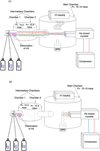 |
Fig. 1 Schematic of the VENUS apparatus: (1) Molecules (H2S and CO) and H atoms (dissociated hydrogen) are injected into the first chamber through the different injection pipes under a pressure of 10−4 mbar. After passing through the second chamber, with a pressure closer to that of the main chamber, the molecules enter the main chamber and are focused onto the gold-coated substrate. While injecting the molecules, the FT-RAIRS records the infrared spectrum of the molecules arriving at the surface of the substrate. This graphical representation of the molecules displays a codeposition of CO, H2S, and H. (2) The FT-RAIRS is stopped and the main chamber is heated while the QMS placed in front of the substrate is on. In this way, all the molecules that sublimate can be recorded by the QMS. |
2.2 Experiments
Two different sets of experiments were performed: (1) hydrogenation of H2S, and (2) reactivity of H2S, CO, and H, in the presence or absence of O2. To quantitatively compare the results from the different experiments, some experimental conditions (i.e., injection of molecular fluxes, quantity of injected molecules, heating process) were kept constant for both sets, while some were varied one at a time (i.e., injection temperature and hydrogenation time). These are detailed below.
The hydrogenation process consists of injecting dissociated H2 at a constant flux of ϕ(H) = 5 ± 1 × 10¹² molecules cm−2 s−1. Furthermore, a constant ramp rate of 12 K min−1 was used to perform the TPD from the deposition temperature to 240 K, recording m∕z from 18 to 66. The amount of desorbed material was calculated by integrating the area for each m∕z curve with the OriginPro 8.0 software2 and comparing the molecular mass spectra from the NIST Webbook Database3.
One of the key species in these experiments is CO. In order to exclude the presence of atmospheric N2 in the chamber (both having a m∕z = 28), we used13CO (m∕z = 29) in our experiments, referenced as CO, instead of 12CO.
For both experimental sets, constant fluxes of ϕ(H2S) = 2.0 ± 0.5 × 10¹² molecules cm−2 s−1 and ϕ(CO) = 1.7 ± 0.5 × 10¹² molecules cm−2 s−1 were used. These fluxes correspond to a time exposure of about 8 min and 10 min for achieving 1 ML on the gold substrate of H2S and CO, respectively.
For the hydrogenation of H2S, that is, {H2S}+{H}, 1 ML of H2S was first deposited on the surface, then H-atoms were sent for 1, 2, 3, 5, 10, and 15 min. These experiments were performed at 10, 30, and 50 K, that is, H2S and H were both injected into the testing chamber at the same temperature. Then the TPD was performed starting from the deposition temperature.
For the reactivity of H2S + CO +H, all the reactants were sent simultaneously on the substrate (hydrogenation included) for 15 min, corresponding to 1.5 ML of H2S and 1.76 ML of CO. Two injection temperatures were tested: 10 and 22 K. These two were chosen as 10 K is the minimum temperature reached by VENUS, and because CO starts desorbing at ~20 K. Testing these two temperatures allowed us to investigate the sensitivity of the H2S reactivity with respect to the low-temperature regime. The laboratory data presented in this paper are from the QMS, therefore the data areonly recorded once all products are on the surface. Detecting the desorption of a species during the hydrogenation is thus not possible from our experimental data set.
Observational details of the SMA and IRAM observations.
3 Observations
The focus of this paper is the study of sulphur chemistry in the cold envelope and the hot core of intermediate-mass protostars of the Cygnus-X complex. For this study, two sets of observations were therefore required to target the cold and hot chemistry with interferometric and single-dish data, respectively. All the observational parameters are summarized in Table 1.
3.1 Observations with the IRAM-30 m telescope
The observations were performed in August 2019 for Cyg X-N12 with a 3 mm line survey from 72.0−79.8 GHz and 84.2−115.5 GHz, using the 30 m telescope of the IRAM facility in Pico Veleta. The broadband EMIR receiver in configuration E090 and the FTS spectrometer in its 200 kHz resolution mode were used for the observations. The weather at the time of the observations was excellent (τ = 0.07 in average), with typical system temperatures of 119 K.
The flux calibration was performed on Uranus and nearby sources K3-50A and NGC 7027, depending on the observing night. The GILDAS 4 software (Grenoble Image and Line Data Analysis Software, Gildas Team 2013) was used for the data reduction and analysis.
Data reduction consisted first of identifying line-free channels by eye. These were then used to subtract a linear baseline from the remaining parts of the spectrum. This was done separately for each spectral range we targeted. The data were brought from the antenna temperature scale to the main-beam temperature scale using a main-beam efficiency, ηMB of 0.81. The noise level was measured from the line-free channels, and was found to be ~3 mK in 0.8 km s−1 channels.
3.2 Observations with the SMA
The submillimeter observations were taken from the PILS-Cygnus survey targeting the ten brightest sources in Cygnus-X complex, observed in June–November 2017. The data were taken with the SMA facility on Maunakea, in a combination of compact and extended configurations for a final resolution of 1′′5. The chosen setup covers the entire frequency range of 329–361 GHz. From this survey, two binary sources were studied, the most massive and luminous one Cyg X-N30 (α = 20h38m36s.6, δ = 42°37′32′′0 [J2000]), and Cyg X-N12 (α = 20h 36m57s.6, δ = 42°11′30′′0 [J2000]), an intermediate-mass protostar that is relatively isolated. Along with frequency coverage, we obtained continuum emission at 0.8 mm wavelengths for both sources. For full details of the observing strategy, data reduction, and cleaning, see van der Walt et al. (2021). The data were reduced and imaged with CASA5 (Common Astronomy Software Applications, McMullin et al. 2007), while line analysis was done with the CASSIS6 software (Centre d’Analyse Scientifique de Spectres Instrumentaux et Synthétiques, Vastel et al. 2015).
4 Results
In this paper, we investigate three approaches to understand the impact of the cold and hot S-chemistry toward protostars: (1) laboratory experiments reproducing ISM conditions and simulating grain S-chemistry in cold conditions, (2) IRAM-30 m observations of the cold envelope of Cyg X-N12, and (3) SMA observations of the hot core of Cyg X-N12 and Cyg X-N30. These observations of protostars allow us to target the S-chemistry in the hot core of intermediate-mass protostars. It was pointed out by van der Walt et al. (2021) that the observed hot core toward Cyg X-N30 is not a traditional hot core, that is, a core in which the gas near the protostar is heated by the accretion luminosity, leading to a jump in the abundance of molecules when the icy mantles sublimate. However, we use the term hot core in this paper to mean the warm gas toward both sources, regardless of their actual physical origin.
4.1 Cold S-chemistry from laboratory experiments
The laboratory experiments were performed in several steps in order to fully understand the behavior of H2S in the presence of CO and H. To determine whether the deposition temperature affects the reactions involving H2S, hydrogenation experiments (i.e., H2S+H) were performed at different deposition temperatures and for different hydrogenation times. The different species were identified based on their mass fragmentation in the QMS. A voltage of 30 eV was used to ionize the desorbing species, a voltage chosen so as to lower cracking (dissociation) of the molecules in the QMS. In turn, this leads to more of the desorbing mass being present in the parent mass, as demonstrated by our group (Nguyen et al. 2019). The recorded final quantity of H2S was found by integrating the primary molecular mass of the component in the TPD spectrum (ATPD), in this case m∕z = 34, and converting it into a fraction with respect to the initial deposition of H2S (equivalent to 1 ML of H2S). The results are displayed in Fig. 2. We observed a strong decrease in the amount of H2S remaining on the surface at 10 K, while at 30 K, the decrease is small (10% decrease) and larger at 50 K, where it decreases to a plateau at ~25% under the maximum.
No products other than H2S and HS were found in the mass spectrum (in particular, no S2, m∕z = 64, or H2S2, m∕z = 66, as shown inAppendix A). The sensitivity limit of the QMS is ~20 cps (counts per second). Therefore, we do not strictly exclude that S2 and H2S2 are formed (both having a desorption temperature below 240 K, i.e., ~140 K for H2S2 and ~230 K for S2; Jiménez-Escobar & Muñoz Caro 2011). If they are present, their signal intensity is ≲10% of the H2S signal, which is not considered as major products of the H2S hydrogenation. We conclude that the loss at 10 K is due to chemical desorption processes (Dulieu et al. 2013). In these processes, the molecules are returned to the gas phase upon the energy released by chemical desorption, as also demonstrated by Oba et al. (2018) in that system. The hydrogenation of H2S leads to a circular solid-state chemistry (H2 abstraction followed by H addition) as outlined here:
 (1a)
(1a)
 (1b)
(1b)
The second reaction, involving two radicals, is very exoergic and is expected to have a very high chemical desorption efficiency (Minissale et al. 2016), whereas the first reaction is less exoergic and therefore is not subject to high chemical desorption efficiency. Reaction (1b) probably has an entrance barrier, in which case the reaction competes with H+H → H2 and H desorption.
At 10 K, the reaction can proceed through diffusive reactivity (the Langmuir-Hinshelwood mechanism), eventually helped by tunnelling effects. At 30 K, the residence time of H on the surface is very low, and even the H+H reaction cannot proceed efficiently on compact amorphous ice (Amiaud et al. 2007). The Eley-Rideal mechanism (direct reaction with an H atom with kinetic energy ~300 K) is still at play. It appears, however, that it is not efficient, especially when taking into consideration that the chemical desorption is efficient for the second reaction, but that this second reaction can also return the initial H2S, and so a looping mechanism is necessary to observe a strong reduction. In contrast, at 50 K we observed a larger disappearance of surface H2S. This is probably due to the desorption of HS. The plateau, made of H2S unreactive molecules, would correspond to the molecules whose orientation of adsorption is not favorable to the Eley-Rideal mechanism. If this interpretation is correct, we can infer an adsorption energy of ~1500 K for the HS molecule, which is more compatible with the value calculated in Oba et al. (2018) (1200 K) than with the value proposed in Wakelam et al. (2017) (2700 K), although admittedly, our method is not very accurate.
In Fig. 3 the quantity of H2S and CO left from the reaction 13CO+ H2S+H is shown at two deposition temperatures, 10 K and 22 K, during a 15 min codeposition. This figure shows that H2S has a highlyreactive behavior when associated with CO, in addition to hydrogenation.
CO hydrogenation (like H2S) has an entrance barrier, and its reactivity, leading to H2CO and CH3OH, is very reduced at 22 K (see, e.g., Watanabe & Kouchi 2002; Fuchs et al. 2009). At 10 K, we first note that if H2S is slightly less consumed inthe presence of CO, the CO reduction is stronger than in case of hydrogenation of CO alone. At 22 K the reduction is stronger for both H2S and CO. This demonstrates cross-linkages between the two hydrogenations, so that HS or HCO are now active reactants in the chain of reactions.
Moreover, this codeposition reaction of H2S, CO, and H shows a larger diversity of products than the sole hydrogenation of H2S. From the recorded mass spectrum of this reaction, several molecules could be traced back according to their individual mass spectrum from the NIST-Webbook database. Several species could be clearly determined, such as H2CO, HCO, OCS, H2S, CO2, and CO. Of these, H2CO and OCS were detected in approximately equal amounts.
H2CO is likely the result of direct hydrogenation:
 (2a)
(2a)
 (2b)
(2b)
Per analogy to the formation of CO2, through the {CO+OH} reaction (Noble et al. 2012; Oba et al. 2018; Ioppolo et al. 2011) via the HOCO intermediate, OCS is possibly formed following this chain of reactions:
 (3a)
(3a)
 (3b)
(3b)
 (3c)
(3c)
To test the strength of the chemical link of CO and HS to form OCS, we conducted one last experiment, introducing some O2 in addition to CO and H2S. O2 reacts with H atoms without barrier, and readily forms OH groups on the surface, which also makes CO2 a final product, and, of course, produces water. The aim of this experiment is twofold: first, we explore conditions more directly related with the interstellar conditions because water formation is probably the main driver of the molecular mantle formation on interstellar dust grains; second, we test the robustness of the previous reaction scheme including a restricted budget of H atoms, as could be the case in dark cloud conditions (Tielens & Hagen 1982). In other words, we study the possibility of OCS formation in a more oxidizing environment.
Under these conditions, we observed a strong production of water, but CO2 and OCS were also produced in almost equal quantity, even though they remained minor products dominated by unreacted CO and H2S, due to a large consumption of H to form water. Nevertheless, we conclude that H2S and CO interactions on solid cold environments produce OCS as a first outcome even in presence of competing reaction pathways whose end-products are H2O, CO2 or CH3OH. Finally, we note here that traces (less than a percent) of many other organo-sulphur compounds may have been found, but their exact composition is hard to determine with mass spectroscopy alone. For example, CS has the same mass as CO2, and isotopologs of C and S complicate the analysis. Nonenergetic pathways or H-driven chemistry in the present case do not showthe same chemical complexity as obtained in energetic experiments (Jiménez-Escobar & Muñoz Caro 2011).
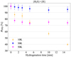 |
Fig. 2 Integrated area of the m∕z = 34 (H2S) curve as a percentage of the initial amount of H2S injected in the experiment at each temperature. The area is calculated from the QMS while performing a TPD, resulting from hydrogenation of 1 ML of H2S during varying time, and at varying deposition temperature of H2S (10, 30, and 50 K). |
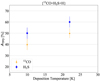 |
Fig. 3 Area of m∕z = 34 (H2S, blue squares in the figure) and m∕z = 29 (13 CO, orange triangles) as a percentage of the initial amount of H2S (1.5 ML) or 13CO (1.76 ML) injected in the experiment during the reaction {H2S + 13CO +H}. The area is calculated from the QMS while performing a TPD. The temperature has been varied (10 and 22 K), while the deposition quantity was kept the same (i.e., corresponding to 15 min of injection). |
4.2 Cold S-chemistry from observations
The line survey of the Cyg X-N12 protostar revealed a rich sulphur environment in its cold envelope. Over the 43 GHz of bandwidth, 55 sulphur-molecular transitions were detected, as shown in Table 2 and listed in Table B.1. Figures C.1–C.3 show parts of the spectrum in which S-lines were identified. The line profiles are narrow (~1–3 km s−1) and Gaussian in nature, as is expected when the profiles trace a single cold, quiescent component; in this case, the cold outer envelope of the protostar.
The sulphur lines detected in this survey (cf. Table B.1) were identified by eye in combination with the CDMS database7 through an iterative process. First, the species already abundantly observed toward protostars were investigated along with their isotopologs. Then, the remaining unknown lines were investigated separately by comparing all possible options with respect to the frequency at which the line was observed by sorting the candidates by their upper level energy (Eup) and Einstein A coefficient(Aij): Eup lower than 150 K and Aij higher than 10−10 s−1 were used as threshold values. When we had several possible candidates, they were investigated over a larger window of the spectrum todetermine whether more transitions were expected according to the CDMS catalog, but were not seen. Conversely, if most of the lines were seen in the spectrum, the candidate was considered as the right molecule. This analysis wasfirst carried out with the WEEDS package from GILDAS (Maret et al. 2011) and confirmed with CASSIS to ensure that each detection was correctly assigned. Using this line identification scheme, a total of 317 lines were identified from 88 different molecules (including isotopologs). Eighteen percent of the total amount of lines we detected still remain unassigned. The species that were not S-bearing will be presented in a forthcoming study.
The optically thin emission from the detected S-molecules were then modeled with the CASSIS software, v.5.1.1. We assumed a local thermodynamic equilibrium (LTE) approximation.
The modeling was done by varying the column density, line width, and excitation temperature (from 7 to 50 K) of the species. The best fit was found by a χ2 optimization model, which is an iterative process based on these parameters. The error margin was determined by running the model four times for the same molecules by changing the intervals over which the parameters were varied and/or number of combinations of the variables (i.e., excitation temperature, line width, column density, and the velocity at local standard of rest).
In this way, the best fit for all detected species was determined. The modeling parameters found for each S-molecule, shown in Table 3, were validated with CASSIS. For some S-species, particularly SO and SO2, a specific modeling could not be realized on all the transitions we saw (i.e., saturation of the column densities for several Tex) because the lines are optically thick. Therefore, the column density of SO was derived from the observed optically thin emission of its isotopolog 34SO, using the isotopic ratio, 32S/34S = 22.5 (Lodders 2003). Only the main isotopolog of SO2 was observed toward the cold envelope: consequently, we were only able to derive lower limits for its abundance, using LTE consideration for a realistic range of excitation temperatures (i.e., 10–40 K). When only one transition was observed (e.g., NS+, NS, HCS+), the excitation temperature was assumed to be 15 ± 5 K. This isthe expected temperature range in the cold envelope, and the ranges on the inferred column densities correspond to this range in excitation temperature. The excitation temperature does not necessarily correspond to the gas temperature, but as we additionally assumed that the level populations are in LTE, this is the best that can be done. Furthermore, for the species with multiple observed transitions, for example, OCS and C3S, we find thatthis excitation temperature is reasonable.
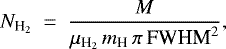
Based on the column density of each species found with LTE modeling and isotopic ratios, we determined their abundances from the ratio of the corresponding column density over the H2 averaged column density,  in the observed region. The latter can be estimated as follows (Hildebrand 1983):
 (3c)
(3c)
where M is the cloud mass,  = 2.8 the mean molecular weight per hydrogen (Kauffmann et al. 2008) molecule, mH the mass of atomic hydrogen, and FWHM is the deconvolved full width at half maximum size.
A mass of 86 M⊙ was determined from single-dish observations assuming no correction for any free-free contamination on the integrated flux, optically thin dust emission, a dust opacity of 0.01 cm−2 g−1 (Ossenkopf & Henning 1994), and a dust temperature of 20 K (Motte et al. 2007). Combining the cloud mass and the FWHM size of 0.1 pc from the single-dish observation of Motte et al. (2007), we find a column density,  , of 1.2 × 1023 cm−2.
Figure 4 displays the abundances of all the detected sulphur species. No specific trend is found among all the abundances, as they vary by up to two orders of magnitude. The highest column densities are seen for the main isotopologs, that is, CS, H2CS, OCS, SO, and SO2, with the latter four showing a similar range of column densities:  /NCS ≈ 1.4 × 10⁻¹, NOCS/NCS ≈ 1.6 × 10⁻¹, NSO/NCS ≈ 3 × 10⁻¹, and
  /NCS ≈ 1.3–3.3 × 10⁻¹.
The lowest column densities are observed for NS+, HSCN, and C3S, with ratios with respect to CS of NNS+/NCS ≈ 9.4 × 10⁻⁴, NHSCN/NCS ≈ 1.1 × 10⁻³, and  /NCS ≈ 2.7 × 10⁻³. There is no apparent correlation between the column densities and whether the species is an organo-sulphur or not.
Detected S-species in the cold envelope of Cyg X-N12.
Overview of the sulphur line LTE modeling for the optically thin emission of Cygnus X-N12 targeting the cold chemistry.
4.3 Warm S-chemistry
The warm chemistry was investigated toward two sources, Cyg X-N12 and Cyg X-N30. These two sources both show multiple continuum peaks (Bontemps et al. 2010; Minh 2016) within the inner few arcseconds. Specifically, the chemistry was investigated toward the peak continuum positions of these two sources alone, whereas the remaining results will be presented in a forthcoming paper (van der Walt et al., in prep.).
The same initial steps as for the cold chemistry survey were performed. First, all the sulphur species were identified from the spectrum ranging from 329 to 361 GHz, with the combination of by-eye identification and verification with the CDMS database over the entire spectrum. However, when analyzing the possible candidates for a certain emission line for the hot-core data, unlike with the cold chemistry, no constraint was given for the upper level energy, while the Einstein coefficient was constrained to Aij higher than 10−10 s−1 as for the cold chemistry. The relevant parts of the spectrum for the S-species are shown in Figs. C.5 through C.7 for Cyg X-N30 and in Figs. C.8 through C.9 for Cyg X-N12.
An overview of the detected S-species toward both sources is listed in Table 4, summarizing the observed molecules, number of lines, and upper-level energy. Complete lists of the detected transitions toward Cyg X-N12 and N30 are provided in Appendix B, Tables B.2 and B.3, respectively. The observed sample consists of 14 different molecular species, 8 of which are isotopologs for Cyg X-N30. Strong lines of several organo-sulphur species could be identified from the 105 lines of sulphur-bearing species, such as H2CS, CS, and OCS. However, they represent only ~18% of the totalS-sample we found, which are mostly dominated by SO, SO2, and corresponding isotopologs. The spectrum of Cyg X-N12 shows a slightly lower diversity of S-molecules, with 12 different species, including 6 isotopologs for a total of 53 sulphur lines we detected. In contrast to Cyg X-N30, the SO and SO2 lines in N12 were weaker and more difficult to detect than the organo-sulphurs (cf. line spectra in Appendix C).
We performed LTE modeling on the optically thin emission of S-species derived from the spectrum at two different locations, MM1a and MM2 for Cyg X-N30 and -N12, respectively (cf. Fig. 6). The modeling parameters and the corresponding error margins were determined in a similar way as for the observations of the cold chemistry, but considering an excitation temperature up to 350 K (cf. Sect. 4.2).
The best-fit parameters found from the LTE modeling analysis we used for the modeling are listed in Table 5. As for the cold-envelope, optically thick emission was seen for the SO and SO2 lines. However, their corresponding isotopologs 34SO and 34SO2 are optically thin, and assuming 32S/34S = 22.5 (Lodders 2003), the expected abundance of SO and SO2 with respect to the averaged H2 column density can be derived. Moreover, the LTE modeling on the observed sulphur-lines toward N30 was found to have similar modeling parameters as those inferred by van der Walt et al. (2021) for the same source.
 was calculated using Eq. (3c). As for the H2 column density estimation of the cold envelope of Cyg X-N12, assumptions of optically thin dust emission and no free-free contamination on the integrated flux were considered. Using a mass of 563 M⊙ derived from 1.2 mm integrated flux, for Cyg X-N30, a FWHM size of 0.1 pc, dust opacity of 0.01 cm2 g−1 and a mean wieght of 2.8, a H2 density of 8× 1023 cm−2 was estimated for Cyg X-N30 (Motte et al. 2007). The same H2 density for Cyg X-N12 as derived in Sect. 4.2 was used for the hot core. The derived H2 column densities for the inner hot core of Cyg X-N30 and N12 were determined from their corresponding large-scale envelope. However, these values are not accurate for the targeted region, the hot core, and we realize that other more accurate values for N30 can be found in the literature (Rygl et al. 2012). We emphasize that the main goal is to determine the trends among the different species, and therefore quoting the exact abundances is not the focus of this paper.
Figure 5 summarizes the abundances of all the sulphur species detected toward both Cyg X-N30 and N12. For both sources, as expected, the highest abundances are seen for SO and SO2, followed by OCS and H2CS, while the lowest abundances are seen for CS and NS. The high abundance of the main organo-sulphur isotopologs, despite their low diversity and poor observed transitions sample, underlines the expected major role of three specific molecules, namely CS, OCS and H2CS. However, we can point out some differences between the two sources: (1) S-column densities observed toward Cyg X-N12 are one to two orders of magnitude lower than for Cyg X-N30. (2) The excitation temperatures of several species tend to be higher for Cyg X-N12, (3) more isotopologs of SO and SO2 are observed toward N30, and (4) the FWHM of the N12 S-O and N-S species are less than half of the widths from N-30 (FWHMSO = 6 km s−1 and FWHMSO = 1.5 km s−1, for N30 and N12, respectively).
Figure 6 for Cyg X-N30 displays the integrated intensity maps (moment-zero maps) for each S-species. As shown by the large number of observed transitions of SO and SO2, the highest integrated intensity (Sν) peaks are observed for these two sulphur-bearing molecules, both peaking at 100–120 Jy beam−1 km s−1. This range is thus considered as the Sν maxima for S-chemistry. A 20–40% lower Sν (~60–80 Jy beam−1 km s−1) relative to the SO and SO2 maxima is observed as maxima of CS and H2CS, and a 40–60% decrease in the Sν peaks (40–60 Jy beam−1 km s−1) is found for OCS and NS.
The spatial distribution of the sulphur species shows some differences depending on the associated molecular family. This was only observed toward Cyg X-N30. The detected S-species are categorized into three families: C-S, N-S, and O-S families. The C-S family contains OCS8, CS, H2CS, and the corresponding isotopologs; the O-S family includes SO, SO2, and the corresponding isotopologs, while NS is the only member of the N-S family. Differences are seen in their peak locations and the overall intensity distribution around their peak.
In Cyg X-N30, the organo-sulphur species in general have a wide central peak and an extended emission distribution, covering the continuum contours nearly uniformly from 2- to 8σ. Their peak regions are elliptical over contours from 2 to 4σ. NS shows a different pattern, with emission toward MM1a and MM1b, two small circular peaks, and a limited spatial extent from 2 to 6σ. The S-O family has a similar pattern, with a spatial extent from 2 to 6σ. Moreover, all the emission is seen to peak toward the N-W from MM1a, while no emission is seen in the N and N-E parts. Their peaks are circular and condensed, extending up to 4σ.
Figure 7 displays the moment-zero maps toward Cyg X-N12. In contrast to Cyg X-N30, the peak intensity maxima of all the species do not exceed ~30 Jy beam−1 km s−1, and no clear differentiation in the range of intensity values is detected among the S-species. The spatial extent of all S-species is similar; the species peak at exactly the continuum peaks, MM1 and MM2. All the species have a circular emission of ~2σ radius around the peak center.
 |
Fig. 4 Abundance of S-species detected toward Cyg X-N12 using the derived S-abundances from Table 3 and |

 |
Fig. 5 Abundance of S-species detected toward the hot-core Cyg X-N30 and Cyg X-N12 using the derived S-abundances from Table 5 and |

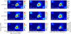 |
Fig. 6 Integrated intensity maps of OCS at 352.6 and 340 GHz, CS at 342.8 GHz and H2CS at 343.4 GHz, NS at 345.8 GHz, SO at 340.7 and at 344.3 GHz, and SO2 at 338.3 GHz and at 348.3 GHz toward Cyg X-N30. The primary binary cores of the Cyg X-N30 are denoted by MM1a and MM1b, while MM2 and MM3 are secondary cores. The right arrow provides the scaling for the intensity of the observed molecule. The red area depicts intensity peaks, and the blue area represents no emission. The contours represent the continuum starting from 2 to 12σ with a spacing of 2σ. The white circle in the bottom left corner represents the beam size. |
Detected S-species in the hot core of Cyg X-N30 and Cyg X-N12.
Overview of the LTE modeling for the optically thin sulphur lines of Cygnus X-N30 and N12 targeting the warm chemistry.
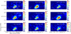 |
Fig. 7 Integrated intensity maps of OCS at 352.6 and 340 GHz, CS at 342.8 and H2CS at 343.4 GHz, NS at 345.8, SO at 340.7 and at 344.3, and SO2 at 338.3 GHz and at 348.3 GHz toward Cyg X-N12. The primary binary cores of the Cyg X-N12 are denoted by MM1 and MM2 (Bontemps et al. 2010). The right arrow provides the scaling for the intensity of the observed molecule. The red area depicts intensity peaks, and the blue area represents no emission. The contours represent the continuum starting from 2 to 10σ with a spacing of 2σ. The white circle in the bottom left corner represents the beam size. |
5 Discussion
In the following, the results of each subpart, the laboratory results, and the observations of the cold and warm S-chemistries are discussed first. Finally, these discussions are synthesized into a summarizing discussion of what has been learned from the combinationof laboratory experiments and observations of S-bearing molecules in different parts of the molecular envelopes surrounding intermediate-mass protostars.
5.1 Laboratory experiments of cold S-chemistry
H2S is highly reactive not only to hydrogenation, but also to CO, resulting in the formation of OCS. These surface reactions were seen at low temperatures (T < 100 K), which suggests that this chemistry occurs already in the cold envelope of the protostars. These are the only regions in which CO will be frozen out on the dust grains.
Variation in the reaction temperature of H2S (15 and 22 K) when mixed with CO and H did not demonstrate a strong effect on the reactivity rate of either H2S or CO. By contrast, with the hydrogenation of H2S alone, a significant variation of H2S left in the sample could be seen from one temperature to another (~35% variation between 10 and 50 K and ~55% variation between 10 and 30 K). The weak temperature correlation implies that the sulphur chemistry leading to organo-sulphur species is produced at a high reaction rate both in the precollapse stage (T ~ 10 K) and in the collapsing envelope (T ≳ 30 K) of the protostar, while the hydrogenation of H2S is efficient only in the precollapse region.
For both reactions, {H2S + CO+ H} and {H2S + CO+ H + O2}, H2S was found as a remaining product. Two possibilities might explain the remaining quantity of H2S in the sample:
The initial [H2S/CO] quantity ratio was too high, and a saturation limit was reached. The initial reactants would not be fully consumed if too few free H atoms remained, explaining the remaining high quantities of CO and H2S in the experimental sample.
The introduced amount of O2 has negatively influenced the reactivity of H2S with CO and H, as these last two species might have more likely reacted with O2 than with H2S. Therefore, it joins the conclusion from point (1), namely too few free H atoms remaining in the sample for the reactivity with H2S to entirely occur.
Our laboratory results allowed us to compare the grain-surface chemistry developed by Laas & Caselli (2019) and Deeyamulla & Husain (2006) to draw a plausible schematic chemical network of the cold chemistry reproduced in the laboratory experiments. To do this, we considered three main species as the starting points of the chemistry (H2S, CO, and O2) reacting principally with H. In this scenario, OCS is the only organo-sulphur produced from the hydrogen abstraction of H2S and combination with CO. The production of OCS among other sulphur species (CS2, H2CS, etc.), in ices containing H2S and abundant C-compounds, that is, CH3OH and CO, was already reported by Jiménez-Escobar et al. (2014) when these ice mixtures were irradiated. The absence of other detected organo-sulphurs is due to the strength of the C=O bond, which requires too much energy (ΔH = 1076.38 kJ mol−1) and cannot be broken by basic surface chemistry. Therefore, it was not included in this experimental setup.
Although it is possible that the amount of O2 in the experiments has negatively affected the quantity of OCS and H2S in the sample by impacting their reactivity, our experiments also suggest that the production of OCS is strongly efficient from H2S on grain surfaces, and the hydrogenation of H2S and CO highly influences its abundance. Our laboratory experiments confirm the efficient hydrogen abstraction mechanism of H2S that was already experimentally observed by Oba et al. (2018) and was modeled by Garrod et al. (2007) and Lamberts & Kästner (2017). This strong hydrogen abstraction mechanism occurring with H2S was initially, and naively, compared to the H2O chemistry as -O is chemically similar as -S to first order, and the same hydrogen abstraction phenomenon occurs. Moreover, for H2O, this H-addition leads to the formation of H2O2, as experimentally tested by Oba et al. (2014) and Miyauchi et al. (2008), but the corresponding S-molecule, H2S2, was not seenfor H2S in a basic surface chemistry without external energy, which suggests that the sulphur chemistry behaves chemically differently from H2O. The formation of H2S2 would thus be formed by UV photochemistry of H2S in a H2O ice-matrix (Jiménez-Escobar & Muñoz Caro 2011; Jiménez-Escobar et al. 2014).
Our study reports the H2S reactivity with CO in a controlled environment. The presence of H2S in the ISM has always been an unresolved challenge (van der Tak et al. 2003; Jiménez-Escobar et al. 2014; Doty et al. 2002; Laas & Caselli 2019). From the modeling side, a high quantity of H2S is predicted on grain surfaces. However, it has not been observed in large quantities so far. Some expect H2S and HS to be S-reservoirs in the ISM (Vidal et al. 2017). Our study demonstrated that when considering H2S already formed and trapped in solid state, H2S will likely rapidly react, leading to the efficient production of organo-sulphur compounds. The reduced sample of organo-sulphurs found in the laboratory is explained by the high enthalpy of C=O bonds. Thus, it is unlikely that H2S remains an S-reservoir on the grains surface. To complete this laboratory study and the derived chemical network, comparison with observational data of the cold envelope of protostars are key.
5.2 Observations of cold S-chemistry
From the number of species we detected, which encompass sulphur species and complex organics, 22% were found to be sulphur molecules, 77% of which can be classified as organo-sulphur species. In the 78% of non-sulphur molecules we found, a large number of zeroth- and first-generation organic molecules as defined by Herbst & van Dishoeck (2009) were detected. These reflect that several orders of reactions have occurred, which was confirmed by the presence of zeroth-generation molecules, such as CH3OH. We therefore expect that the observed S-species are also zeroth- and first-generation species, but that their actual abundances depend on both the evolutionary stage of the protostar and the location within the protostellar envelope. They also underline the high reactivity in the targeted environment due to the freeze-out of the molecules on the dust grains.
This study focuses only on the chemical pattern formed from surface chemistry on dust grains, considering only the environmental conditions (i.e., temperatures) to vary and high freeze-out rate (i.e., the hydrogen number density >105 cm3; Schmalzl et al. 2014). Therefore, it is assumed that grain properties such as the composition, sizes, and distribution of grains and the nonporous grain surface are constant and do not influence the S-reactivity.
Moreover, the large diversity of organo-sulphurs and the total column density ratios of the detected organo-sulphurs (OS) and non-organo-sulphurs (NOS) (i.e., ∑ N(NOS)/∑ N(OS) = 0.29) suggest thatthis trend indicates that a large fraction of S is locked up in organo-sulphurs. It emphasizes an efficient chemistry with organic compounds in the gas-phase and on dust grains in the cold environment (10–30 K), as is found in the collapsing envelope (Laas & Caselli 2019).
The highest inferred abundances are seen for CS, OCS, H2CS, SO, and SO2. From a chemical point of view, both the S-O and C-S families are thus considered good tracers of the cold envelope. We might rely on the diversity observed in S-molecules and on targeting the cited main isotopic S-molecules, specifically CS, as tracers for the cold envelope assuming a homogeneous chemistry throughout the envelope, as suggested observationally by van der Tak et al. (2000) and Jørgensen et al. (2004) and based on models by Doty et al. (2002).
The high abundance of SO and SO2 was unexpected as these molecules are known to trace warm gas, such as toward the hot core and outflow or jet regions (Singh & Chakrabarti 2012; Minh 2016; Artur de la Villarmois et al. 2019). The high abundance and low diversity of S-O molecules suggest thatthese molecules are produced already in the cold envelope from oxidation of atomic S on the dust grains. Here they remain intact and do not proceed to form more complex products. The desorption of these species at low temperatures might result from nonthermal processes such as photodesorption, sputtering, and reactive desorption. Photodesorption occurs whenthere is local heating of the grain surface induced by external irradiation (e.g., UV, X-ray; Westley et al. 1995; Öberg et al. 2009). The sputtering is also an efficient nonthermal process. In this case, particles collide with the grain surface, inducing strong enough kinetic energy to desorb the species present on the grain, while the reactive desorption refers to the energy released by the chemical reactions, leading to the desorption of the species (Vasyunin & Herbst 2013). However, at this stage, it is unknown which process dominates the desorption of SO and SO2 in this cold environment. These three mechanisms provide a means for releasing S-O molecules into the gas phase even in the cold parts of the envelope, however.
5.3 Observations of warm S-chemistry
The interferometric observations of the hot core enable not only investigating the molecular diversity, but also the spatial distribution of their emission. This analysis, performed for the peak continuum positions toward Cyg X-N12 and N30, shows that similarities and discrepancies of the S-chemistry in the warm gas could be distinguished between the two sources.
From the spectral analysis, similarities between the spectral line surveys toward the two sources Cyg X-N12 and N30 could be deduced from the observations. In particular, the diversity of organo-sulphurs is low, as only OCS, H2CS, and CS are detected, in contrast to the S-species observed in the cold envelope of Cyg X-N12. This reduced diversity toward Cyg X-N12 and N30 is also observed toward the well-studied low-mass protostar, IRAS 16293–2422B by Drozdovskaya et al. (2018), and was used in hot-core models of Vidal & Wakelam (2018). Therefore, the concordance among the detected organo-sulphurs toward Cyg X-N12 and N30, IRAS 16293–2422B and models makes it unlikely that N12 and N30 are possible outliers in terms of hot-core S-chemistry. This also suggests that the diversity of organo-sulphurs in the warm gas is not dependent on the mass of the protostar. However, more sources must clearly be observed to verify this conclusion.
The only organo-sulphurs detected in the warm gas, OCS, H2CS, and CS, also show the highest column densities of the organo-sulphurs in the cold envelope of N12 ( = 1.3
= 1.3 × 1014 cm−2, NOCS = 1.5
 × 1014 cm−2, NCS = 9.0
 × 1014 cm−2). Moreover, their column densities in the warm gas are one order of magnitude higher than in the cold gas. Therefore, the detected organo-sulphurs in the warm gas might partially originate from the cold envelope, collapsing toward the hot core, as they have likely been efficiently produced in the cold environment from successive hydrogenations and oxidations of atomic sulphur. The remaining organo-sulphurs we detected might then be produced in the warm gas.
Consequently, for sources N12 and N30, we investigated the nondetection of the organo-sulphurs that were detected in the cold envelope of Cyg X-N12, but not in thet wo hot cores (i.e., CCS, C3S, CH3SH, and HSCN).We used the CASSIS software to build synthetic spectra and determine upper limits. In order to determine an upper limit, the excitation temperature was first fixed such that it matched the averaged temperature found from the main species in the same molecular family, in this case, the C-S family. For N30, this temperature is 190 K, and for N12, it is 160
 K. Next, we varied the column density of these species, and the resulting spectrum was investigated across the spectral range. When a simulated emission line appeared at the 3σ level, that is, above the noise level, the corresponding column density was taken as the 3σ upper limit. This was done forCCS, C3S, CH3SH, and HSCN, and their values are given in Table 5. Typically, they are 1015 –1016 cm−2. The formation routes of these species were also later investigated and shown in Fig. 9, and a further discussion of the upper limits is provided in Sect. 5.5.
Of all S-molecules we detected, those observed toward Cyg X-N30 have higher column densities than those toward N12 (Nsp-N30/Nsp-N12 = 10–102). These are explained by N30 being 33.8 times brighter than N12 (Lbol = 740 L⊙, LFIR=33.8 × 10³ L⊙ for N12; Pitts et al., in prep.) and more massive (M = 563 M⊙ for N30 and M = 86 M⊙ for N12; Motte et al. 2007). Therefore, for a given sensitivity, the column densities of the S-species are sensitive to the mass of the observed protostar.
The highest abundances of S-species toward Cyg X-N12 and N30 are seen for SO and SO2, confirming that these are good sulphur tracers of the warm chemistry of protostars, as previously suggested by van der Tak et al. (2003) and Artur de la Villarmois et al. (2019), for example. Moreover, these two molecules show the largest differences in column densities between the cold envelope (c) and hot core (h) of N12, with  /
/ ≈ 81 and
  /
/ ≈ 180, while for the organo-sulphurs, we found lower variations between the cold and warm chemistry:
  /
/ ≈ 39,
≈ 39,  /
/ ≈ 28 and
  /
/ ≈ 1.4. These large differences might underline that the observed SO and SO2 in the hot core do not only come from the collapsed envelope, but are also produced in the warm gas.
An interesting difference appears in the FWHM of the organo-sulphurs when compared to the non-organo-sulphur species toward the two sources. For both sources, the FWHM of the organo-sulphurs is similar, ~4–5 km s−1. However, for N30, the non-organo-sulphurs show an increase in the FWHM to ~6.0–6.5 km s−1, whereas this decreases toward N12 to 1.5–2.0 km s−1 for most species. This difference in line widths between the sources might indicate a slower motion in the hot core of Cyg X-N12 than N30. The non-organo-sulphurs appear to be more sensitive to the motion of the protostars, although a survey of more sources at higher angular resolution is required to clearly demonstrate this effect. N30 is more massive than N12, and gravitational collapse should therefore occur faster (Klassen et al. 2016).
High column densities were observed for OCS and H2CS in both protostars (i.e., NOCS = 1.4 1017 cm−2,
  = 2.4
= 2.4 1016 cm−2 for N30 and NOCS = 5.9
 1015 cm−2,
  = 3.7
= 3.7 1015 cm−2 for N12), thus making them good tracers of the warm chemistry as well. As pointed out previously, it is plausible that the high abundances of OCS and H2CS observed in the hot regions are related to the cold chemistry through the collapsing envelope (Wakelam et al. 2011; Jørgensen et al. 2004, and references therein), as these have relatively high column densities in the outer envelope (cf.
  /
/ ≈ 39,
≈ 39,  /
/ ≈ 28 for N12).
For the case of H2CS, the extensive models of the sulphur chemistry in hot cores from Vidal & Wakelam (2018) and Vidal et al. (2019) suggested that at T ~100 K, H2CS has not entirely desorbed from the surface and its abundance depends on the surface and gas-phase chemistries. In their model, H2CS is likely to be produced by the following reactions:
 (5a)
(5a)
 (5b)
(5b)
 (5c)
(5c)
while the destruction of H2CS occurs on the dust grain and in the gas phase, as shown by the following reactions:
 (6a)
(6a)
 (6b)
(6b)
 (6c)
(6c)
 (6d)
(6d)
in which the subscript (s) denotes the solid state of the species, that is, reactions on the dust grain. Furthermore, H3CS+ formed in Eq. (6a) re-forms to H2CS from the dissociative recombination of H3CS+ with e−. At higher temperatures (T ~ 300 K), H2CS is entirely inthe gas phase, and its only destruction paths are described by Eqs. (6a) and (6b). Therefore, H2CS in the hot core is not necessarily destroyed as it re-forms through H3CS+ and the low abundance of atomic carbon does not lead to a highly efficient destruction path of Eq. (6b). This might explain the high H2CS abundance in the warm gas.
In the case of OCS, the models from Vidal & Wakelam (2018), Vidal et al. (2019) and Druard & Wakelam (2012) predict a high abundance of OCS due to its production on grain surfaces and in the gas phase through the following set of reactions:
 (7a)
(7a)
 (7b)
(7b)
 (7c)
(7c)
 (7d)
(7d)
 (7e)
(7e)
 (7f)
(7f)
while its destruction is expected to occur through several paths, as outlined here:
 (8a)
(8a)
 (8b)
(8b)
 (8c)
(8c)
 (8d)
(8d)
However, Eqs. (8b) and (8c) produce HOCS+, which will dissociatively recombine to form either CS or OCS, and Eq. (8d) is expected to be efficient for only the first 10 years of the simulation, due to the low abundance of atomic C. Furthermore, at high temperatures (T ≈ 300 K), the drop in CH abundance leads to an inefficient OCS destruction from Eq. (8a). Therefore, the low destruction rates of OCS compared to its production rates might explain its high abundance in the warm gas.
Furthermore, the same high column densities for OCS, SO CS, SO2, and H2CS were observed for IRAS 16293-2422, for which the derived density ratio NCS/NOCS ≈ 10−1 describes a lower density of CS than OCS (Le Gal et al. 2019; Drozdovskaya et al. 2018). The same trend is observed for the warm gas of N30 and N12, which has ratios of NCS/NOCS ≈ 0.07 and NCS/NOCS ≈ 0.22 for N30 and N12, respectively. If CS is optically thin, these density ratios found toward IRAS 16293-2422, Cyg X-N12, and N30 suggest that OCS production is more effective in the warm gas than the CS production, in contrast to what is seen for the cold envelope of N12 (NCS/NOCS ≈ 6).
From the moment-zero maps from the sulphur emissions toward Cyg X-N30, a similar trend could be observed for the S-species within a specific S-family. As illustrated in Fig. 8, the distinction among families is based on the S-peak location andon the spatial extent of the S-emission.
In all the S-species we detected, their peak emission is shifted from the continuum sources, MM1a and MM1b. In the S-O and N-S families as well as for CS, their intensity peaks have a shift of ~0′′75, ~0′′2, southwest of MM1a, while other species of the C-S family have a shift of ~0s.2, ~0′′2, northeast of MM1a. This peak shift from MM1a is observed for all the COMs of Cyg X-N30, as discussed by van der Walt et al. (2021), and is likely explained by N30 not being a traditional hot core, in contrast to N12.
Despite the emission peak shifts for N30, a specific and different spatial distribution of all S-species was seen in the families. The organo-sulphurs show an extended pattern around the two binary components (MM1a and MM1b), their spatial distribution is more extended and not concentrated on a specific source, in contrast to the O-S family, which is concentrated around MM1a, as also pointed out by van der Walt et al. (2021). It might be suggested that C-S is associated with both sources (i.e., MM1a and MM1b), while the O-S family is primarily associated with MM1a. Only one molecule could be identified in the N-S family (NS). It is not possible to draw clear conclusions regarding an entire S-family based on only one species. However, as the two other families show the same characteristics for all their species, it is likely that the molecules within the N-S family follow the same trend, as also observed for N-species, CH3CN, HC15N, HC3N, and HNCO in N30 by van der Walt et al. (2021).
This differentiation in molecular spatial distribution has already been discussed by Garrod & Widicus Weaver (2013), who suggested that it is correlated with changes in local physical conditions. Differentiation in spatial extent is also seen for N- and O-bearing molecules in Orion KL, which are likely to trace separate physical environments (Favre et al. 2011; Weaver & Friedel 2012; Zapata et al. 2011; Friedel & Snyder 2008; Crockett et al. 2015; Pagani et al. 2017). Furthermore, Neill et al. (2011) discussed this difference in spatial extent as a possible consequence of gas-phase reactions that might alter the initial spatial distributions. This initial spatial distribution is created by similar physical mechanisms (e.g., molecular desorption from the dust grains, shocks); however, in the subsequent gas-phase reprocessing, the limiting reactants set any further chemical processing, and these reactants are typically the less-abundant species. Both explanations might be applicable for Cyg X-N30, namely that the chemical gradient traces a physical gradient in temperature, density, or other physical parameters, but it is likely not the cause of this gradient in physical properties, but rather a consequence of it. Moreover, a wider spatial extent was seen for the C-S family in which the organo-sulphurs have a lower abundance than O-S species, probably explaining the stronger effect on their spatial extent (Neill et al. 2011).
Although the line analysis and derived abundances show similarities between Cyg X-N12 and N30, their moment-zero maps show different patterns. It is clear that for both sources, Cyg X-N30 and N12, the diversity of S-species is similar for the warm gas. Furthermore, a similar trend between the sources is also seen for the abundance ratios. However, for Cyg X-N12, Fig. 7 shows that the spatial distribution for the same angular resolution does not differ among the species, in contrast to N30. This suggests that the spatial extent of the sulphur molecules depends on the type of object that is targeted (e.g., traditional hot core or not) and not on the region (cold envelope versus hot core). In the case of a traditional intermediate-mass source as N12, the molecular emission is expected to only overlap with the continuum emission, while for atypical sources (e.g., N30, Orion KL), the spatial distribution provides information on the type of sulphur species and physical environment of the warm gas (Favre et al. 2011; Weaver & Friedel 2012; Neill et al. 2011).
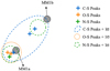 |
Fig. 8 Cartoon of the locations of sulphur species characterized w.r.t. chemical families (i.e., N-S, O-S and C-S) of Cyg X-N30 around the MM1 source. Concentrations of the sulphurs peaks located in specific regions depending on the corresponding sulphur family. Results from the SMA-PILS Cygnus survey. Cyg X-N30 was observed at 0.8 mm. |
5.4 Combining the cold S-chemistry from the observations and the laboratory
The results from the laboratory do not entirely match the observational results of the cold envelope of Cyg X-N12, as the only sulphur species detected in the laboratory was OCS, while the cold envelope displays a large diversity of organo-sulphurs. The high amount of H2S left in the sample (~8%) suggests that the chemical reactions are not completed and longer exposition to H would lead to a larger quantity of OCS. Moreover, the absence of a strong energy source such as a UV field would be one factor limiting the reactivity of our experiments, but not the only principal cause affecting the diversity of organo-sulphurs we found. However, in a cold environment such as the cold envelope, the UV field is not strong, and therefore this absence of UV is more characteristic of such a cold environment. We emphasize here that the laboratory experiments display the products from the grain surfaces chemistry, while the observations of the cold envelope display the products resulting from the gas-phase chemistry and from the desorption of species produced on the dust grains. Both occur in the cold envelope simultaneously and are thus complementary. However, they cannot be directly compared without knowing the (nonthermal) desorption yields, and these are at present unknown for the S-bearing species.
Combining the observational results with our laboratory knowledge, a schematic chemical network for the grain chemistry in cold environment is inferred. We based the reactions on those that were demonstrated by Vidal et al. (2019, 2017), Vidal & Wakelam (2018), Laas & Caselli (2019), Vastel et al. (2018) and Deeyamulla & Husain (2006) and references therein. The chemical network is shown in Fig. 9 and represents a possible path for the production of S-species in star-forming regions. It is important to underline that this chemical network does not target a specific chemistry (i.e., warm or cold chemistry), but provides an overview of the reactions leading to the S-species.
This version of the chemical network from the laboratory points out the experimental limitations, but highlights the link between OCS and the other organo-sulphurs, as well as the central role of H2S in the sulphur chemistry. The reason for this is that one of the main dissociation products of H2S is HS, which has a high reactivity, both on the grain and in the gas. As shown in Fig. 9, external energy (e.g.,UV radiation) would be required for the production of some of its daughter molecules such as CS, C2S, C3S, and H2CS, which would be expected to be formed from the photodissociation of C=O bonds from OCS or its reaction with C or CH. Furthermore, the production of OCS from HS and CO found from the laboratory experiments contradiction the results from Laas & Caselli (2019), which describes this reaction as not allowed, and Vidal et al. (2019), in which the main production route for OCS on the grain surface is from Eq. (7f). This new production route of OCS on the grain surface requires further theoretical investigation.
Due to the high reactivity and abundance of CO and H in the ISM, the abundance of the initial reactants of this network (e.g., H2S) is expected to be low and thus be revealed through reservoirs of their products (OCS, HCS, etc.). Thus, the initial abundance of H2S may be inferred from its products (OCS and CS) as detected in the envelope, and this molecule is a zeroth-generation molecule (Herbst & van Dishoeck 2009). H2S is a primary reactant of the S-chemistry, it is not considered as a good tracer of the cold chemistry, as most of the H2S is expected to react with H and dissociated C=O, thus lowering its abundance. One should focus instead on the subsequent S-reservoirs (primarily OCS, then CS, H2CS, etc.) to derive its initial abundance in the early stage of the protostellar evolution. However, H2S is considered as a primary component of S-chemistry in this region due to the large amount and type of organo-sulphurs we detected, which is expected to result from H2S and CO hydrogenation as found from the laboratory experiments.
In the observational data, the highest column density of the detected species is seen for CS in the cold envelope, underlining that CS is efficiently produced, as also suggested by Palumbo et al. (1997), by different production routes. The main routes of CS are from the reactions of S with C2 and CH (Vastel et al. 2018) as well as the electronic dissociative recombination of HCS+ with e−. However, as described by Eqs. (8d), the chemical reaction in the gas state producing CS from OCS is possible, but not exclusive (Vidal & Wakelam 2018; Deeyamulla & Husain 2006).
5.5 Combining warm and cold S-chemistries
The observations presented in this paper connect the sulphur chemistry through the warm and cold environment among intermediate-mass protostars of the Cygnus-X star-forming complex. The largest diversity of S-molecules is observed toward the cold envelope. This suggests that the outer part of the protostar contains all the possible S-species that play a role in its chemistry. Moreover, the limited diversity in S-species in the warm gas (i.e., hot-core regions) found toward N12 and N30 has also been observed for other sources such as IRAS 16293–2422B and was used in hot-core models (Drozdovskaya et al. 2018; Vidal & Wakelam 2018). As specified previously (see Sect. 5.2), the cold envelope is the coolest part of the protostellar system, the combination of the dust and low temperature allows a rich surface chemistry to occur, and most of the molecules are thought to principally form on dust grains at low temperatures (Jørgensen et al. 2020).
The larger diversity of S-molecules in the cold envelope compared to the hot core does not automatically imply that the four nondetected S-species, CCS, C3S, CH3SH, and HSCN, in the hot core are not there. To determine whether they may be present in the hot core, the upper limits of their column densities were investigated. A comparison of the column densities in the cold envelope (c) and hot core (h), of these nonobserved S-species with respect to CS was made for N12. The same ratio  /
/ = ≈ 1 for all these species was found in the hot core as the same upper limit for them was derived, while different ratios were found for the cold envelope:
  /
/ =
= /
/ 10−2 and
  /
/ =
= /
/ 10−1.
10−1.
When comparing the ratios from the cold envelope and the hot core, we used OCS as a reference frame. In Table 6 we show the column-density ratios for the detected and nondetected species for the cold envelope and the hot cores of N12 and N30, respectively. The detected species all show similar column density ratios within a factor of a few, which suggests that the chemistry in the cold envelope and the hot cores of these different species does not vary significantly. This suggests that the sulphur chemistry in the hot core is to a high degree inherited from the cold envelope. At the upper limits, the sensitivity of the observations is clearly too low for N12 for us to conclude anything: the nondetections are consistent with a scenario in which the species are inherited from the cold envelope with the same column-density ratio. For N30, on the other hand, we find that CCS, C3S, and CH3SH should have been detected if their column-density ratios follow the other ratios. This suggests that their abundance may be chemically lowered either on the way to the hot core or in the hot core itself. As this difference is not driven by sensitivity issues, the conclusion is that the sulphur chemistry is best studied in the cold envelope, where the observed diversity of species is highest.
Based on the derived column densities, our results match previous observational conclusions (Artur de la Villarmois et al. 2018, 2019; van der Tak et al. 2003; Wakelam et al. 2011), that is, CS is considered as the main tracer for the cold chemistry, with the highest column density of NCS = 9.0 ×1014 cm−2, and SO and SO2 as primary tracers for the warm chemistry, NSO = 1.3
 ×1018 cm−2,
  = 1.3
= 1.3 1018 cm−2. However, forthe cold envelope, the SO and SO2 abundances were among the five highest abundances of the 11 detected S-species, and thus were also considered as tracers of the cold envelope. The ratio of NCS/NSO or NCS/
 might thereofre be considered to precisely determine the environmental conditions rather than focusing on the column density of a specific species. If the ratios are higher than one, then this is likely to be the outer part of the protostar, and inversely, ratios lower than one target the inner part of the protostars. Furthermore, this ratio has also been suggested by Bergin et al. (1997) to probe the C/O ratio in the targeted region, as the main production route for SO is from atomic sulphur and oxygen. This is in accordance with our use of this ratio, as in the cold envelope, the atomic oxygen is efficiently converted into H2O on grains and thus its abundance in the gas is depleted, while at higher temperatures, that is, in the hot core, the released oxygen from the ice desorbs and forms more S-O species, which explains the higher densities of S-O species in the warmer chemistry.
The comparison of column densities also indicates the opposite trend in the cold and warm chemistries for CS and OCS. These species are directly related, as shown in Fig. 9. Their abundances in the cold envelope and hot core of N12 and N30 suggest that in a cold environment, the production of CS is enhanced by OCS through reactivity with carbon. By contrast, in the warm gas, the opposite route seems to occur, namely CS combines with OH to form OCS in the gas phase (Vidal & Wakelam 2018). Moreover, in the warm gas, the high abundance observed for OCS is likely caused by a combination of gas chemistry and the thermal desorption of OCS from the icy dust grains, formed in the cold envelope, as suggested by the laboratory experiments.
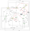 |
Fig. 9 Sulphur solid- and gas-state chemical network derived from laboratory experiments, observational study of Cyg X-N12 and N30 (i.e., S-species observed in the cold- and warm-gas chemistries), and previous theoretical studies from Vidal et al. (2019, 2017), Vidal & Wakelam (2018), Laas & Caselli (2019), Vastel et al. (2018) and Deeyamulla & Husain (2006). The products found in the laboratory are highlighted in the blue boxes, and the species from the observation of cold gas of Cyg X-N12 are shown inside the dotted green boxes. The species detected toward Cyg X-N12 and N30 in the warm gas are shown inside the orange boxes. The straight lines represent the reactions with an additional reactant, shown by the plus. The dotted line represents the reaction found from the laboratory experiments. The gas-phase reactions are shown by black arrows, and the red arrows indicate the solid-state chemistry. |
Comparison between cold envelope and hot core of species with respect to OCS toward N12 and N30.
6 Conclusions
To improve our knowledge of the sulphur chemistry in star-forming regions, we studied the cold and hot chemistries in a rich molecular complex of our Galaxy, Cygnus X. Two protostars from this complex were targeted based on their high luminosity, mass, and relative isolation from other sources. The observations were supported by laboratory experiments focusing on the H2S chemistry. The main findings of this paper are summarized as follows:
H2S shows a high reactivity when exposed to CO and H in a cold environment without any additional source of energy, leading mainly to the production of one organo-sulphur: OCS. Moreover, its reaction efficiency is not highly sensitive to variations in temperature over a range of 10–50 K.
H2S appears to be a possible starting point of the reaction chain of sulphur chemistry and therefore is considered as the primary component for the S-chemistry. Being at the start of chemical reaction chain, its initial abundance can only be derived from its products. Thus, it cannot be considered a good tracer for the cold chemistry of a star-forming region: the focus should instead lie on its product, for instance, OCS.
The cold envelope hosts a large diversity of S-species, mostly organo-sulphurs. Only OCS of the observed organo-sulphurs is also expected to be formed on the icy dust grains, as suggested by the laboratory experiments, from H2S reacting with CO and H. The remaining organo-sulphurs correspond to products from expected later stages of reactions of the CS chain. The diversity of organo-sulphurs we detected is a clear indicator that the sulphur chemistry has had time to evolve.
The highest S-species abundance in the cold envelope is observed for CS, which is expected to be efficiently produced by different routes in the gas phase, but also on grain surfaces (cf. Fig. 9). The S-chemistry in the cold envelope is primarily led by reaction chains from CS, and this species is considered the main molecular tracer of the cold envelope regarding the S-chemistry.
An unexpectedly high abundance of SO and SO2 was observed in the cold envelope, although these are typically used for tracing warm chemistry, that is, the hot core and outflows. Their high abundance and the low diversity of S-O molecules reveal that these molecules are produced in the cold envelope, but do not react with the surrounding environment and are seen in hotter regions due to the collapsing envelope.
Although SO and SO2 could clearly be detected in the observations, the diversity of the sulphur sample in the hot core is poor. Only three organo-sulphurs, OCS, H2CS, and CS, are detected toward both sources. Although the abundance of the other organo-sulphurs (CCS, C3S, and CH3SH) is too low to be detected toward N12, these species should have been detected toward N30 if the chemistry is similar toward both N12 and N30. This in turn suggests that the abundance of these species decreases toward the hot core of N30.
We observed high abundances of the organo-sulphurs OCS and H2CS, which might also be considered good tracers of the warm chemistry. It is likely that the high abundance of OCS in the hot core is due to its nonthermal and thermal desorption from the icy dust grains. Their high observed abundance compared to CS arises because they are produced on the surface but also in the gas phase of the hot core and are not easily destroyed (cf. Eqs. (6a), 7, and (8b)).
The spatial distribution of S-species within the hot-core region depends on the targeted object. For the typical hot core of a protostar, no differentiation is expected among the S-species, while for more massive objects with a nontraditional hot core (i.e., Cygnus X-N30), the spatial distribution provides information on the type of S-species and on the physics and chemistry within the hot core.
In conclusion, this study allowed us to confirm for the first time from a laboratory perspective that OCS is more likely to be a solid-state S-reservoir than H2S, the latter being expected to be a key solid-state reactant of the sulphur chemistry in protostellar envelopes. The observational spectral surveys covering a large bandwidth provided us with a complete outlook on the S-species in different regions of intermediate-mass protostars. This allowed us to point out similarities and discrepancies among the warm and cold S-chemistry of these astrophysical objects. Moreover, we determined that the chemical S-inventory and the derived abundances are dependent on and characteristic of the environmental temperatures, while its spatial extent depends on the type of object that is targeted. Extending this analysis to a larger set of protostars is required to confirm that the trends observed in Cygnus X-N12 and N30 are characteristic of protostars. Such an extension would naturally also benefit from an increase in sensitivity, that is, detecting more species in the hot cores, and in angular resolution to follow the sulphuric gas flows near the protostars.
Acknowledgements
We would like to thank the anonymous referee for the thoughtful suggestions that helped to improve this manuscript. This work was supported by the Programme National “Physique et Chimie du Milieu Interstellaire” (PCMI) of CNRS/INSU with INC/INP co-funded by CEA and CNES, by the DIM ACAV+ a funding program of the Region Ile de France, and by the ANR SIRC project (GrantANR- SPV202448 2020-2024). The research of MeA, LEK, RP, and SvdW is supported by a research grant (19127) from VILLUM FONDEN. This work is based on observations carried out under project number 035-19 with the IRAM 30 m telescope. IRAM is supported by INSU/CNRS (France), MPG (Germany) and IGN (Spain). The Submillimeter Array is a joint project between the Smithsonian Astrophysical Observatory and the Academia Sinica Institute of Astronomy and Astrophysics and is funded by the Smithsonian Institution and the Academia Sinica. We acknowledge and thank the staff of the SMA for their assistance and continued support. The authors wish to recognize and acknowledge the very significant cultural role and reverence that the summit of Mauna Kea has always had within the indigenous Hawaiian community. We are most fortunate to have had the opportunity to conduct observations from this mountain.
Appendix A Laboratory temperature desorption profile
This appendix shows one of the temperature-programmed desorption profiles we used for this study. It provides an overview of the mass decomposition observed by the QMS. In Figure A.1 we show the hydrogenation of the H2S at 10 K during 15 min. The data were rebinned by a factor of 4 for clarity, such that the temporal resolution is 4 sec as opposed to 1 sec (in temperature units, this difference 0.8 K vs. 0.2 K). Results are shown for values of m∕z of 32 (S), 34 (H2S), 36 (H S), 64 (S2), and 66 (H2S2 or S34S). The secondary peak for m∕z = 34 (H2S) at ~ 140 K is likely caused by a small amount of H2S that is trapped in H2O, which desorbs at this temperature. For m∕z = 64 and 66, the spectra were multiplied by a factor of 3 to illustrate the nondetections at high temperature. Both molecules have desorption temperatures below 240 K (Jiménez-Escobar et al. 2014).
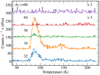 |
Fig. A.1 Temperature-programmed desorption profiles obtained after hydrogenation of H2S at 10 K for 15 min. The TPD is performed from 40 K to ~220 K, and the values of m∕z are shown for each spectrum (see the main text for the species to which they correspond). The spectra have been rebinned by a factor of 4 for clarity, and are offset from one another by 80 counts s−1. |
Appendix B Line identification
Tables B.1–B.4 list all the molecules we detected toward CygX-N12 and N30 in the cold and warm chemistries, as well as their transition and upper-level energy.
Detected S-species toward CygX-N12. Cold chemistry
Detected S-species toward CygX-N12. Warm chemistry
Detected S-species toward CygX-N30. Warm chemistry
Appendix C Line spectra
The spectra of the cold envelope and hot core of CygX-N12 are shown in Figures C.1-C.4and C.8-C.9, respectively. The spectra of the hot core of N30 are displayed in Figures C.5-C.7. The detected S-species are shown in all the spectra.
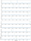 |
Fig. C.1 Spectrum in the range 72.2–86.9 GHz toward the source CygX-N12. Transitions of the sulphur species are identified. |
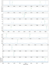 |
Fig. C.2 Spectrum in the range 90.62–99.8 GHz toward the source CygX-N12. Transitions of the sulphur species are identified. |
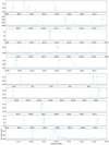 |
Fig. C.3 Spectrum in the range 100–113.7 GHz toward the source CygX-N12. Transitions of the sulphur species are identified. |
 |
Fig. C.4 Spectrum in the range 115–115.4 GHz toward the source CygX-N12. Transitions of the sulphur species are identified. |
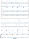 |
Fig. C.5 Spectrum in the range 329.2-340 GHz toward the source CygX-N30. Transitions of the sulphur species are identified. |
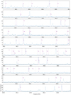 |
Fig. C.6 Spectrum in the range 340-352 GHz toward the source CygX-N30. Transitions of the sulphur species are identified. |
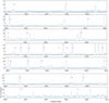 |
Fig. C.7 Spectrum in the range 352-361 GHz toward the source CygX-N30. Transitions of the sulphur species are identified. |
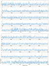 |
Fig. C.8 Spectrum in the range 330-344 GHz toward the source CygX-N12. Transitions of the sulphur species are identified. |
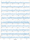 |
Fig. C.9 Spectrum in the range 344-360.5 GHz toward the source CygX-N12. Transitions of the sulphur species are identified. |
References
- Amiaud, L., Dulieu, F., Fillion, J.-H., Momeni, A., & Lemaire, J. 2007, J. Chem. Phys., 127, 144709 [NASA ADS] [CrossRef] [Google Scholar]
- Artur de la Villarmois, E., Kristensen, L. E., Jørgensen, J. K., et al. 2018, A&A, 614, A26 [NASA ADS] [CrossRef] [EDP Sciences] [Google Scholar]
- Artur de la Villarmois, E., Jørgensen, J. K., Kristensen, L. E., et al. 2019, A&A, 626, A71 [NASA ADS] [CrossRef] [EDP Sciences] [Google Scholar]
- Asplund, M., Grevesse, N., Sauval, A. J., & Scott, P. 2009, ARA&A, 47, 481 [Google Scholar]
- Bergin, E. A., Goldsmith, P. F., Snell, R. L., & Langer, W. D. 1997, ApJ, 482, 285 [NASA ADS] [CrossRef] [Google Scholar]
- Bontemps, S., Motte, F., Csengeri, T., & Schneider, N. 2010, A&A, 524, A18 [NASA ADS] [CrossRef] [EDP Sciences] [Google Scholar]
- Boogert, A. C. A., Gerakines, P. A., & Whittet, D. C. B. 2015, ARA&A, 53, 541 [Google Scholar]
- Buckle, J. V., & Fuller, G. A. 2003, A&A, 399, 567 [NASA ADS] [CrossRef] [EDP Sciences] [Google Scholar]
- Charnley, S. B. 1997, ApJ, 481, 396 [NASA ADS] [CrossRef] [Google Scholar]
- Congiu, E., Sow, A., Nguyen, T., Baouche, S., & Dulieu, F. 2020, Rev. Sci. Instrum., 91, 124504 [NASA ADS] [CrossRef] [Google Scholar]
- Crockett, N., Bergin, E., Neill, J., et al. 2015, ApJ, 806, 239 [NASA ADS] [CrossRef] [Google Scholar]
- Deeyamulla, M., & Husain, D. 2006, J. Photochem. Photobiol. A Chem., 184, 347 [Google Scholar]
- Doty, S. D., van Dishoeck, E. F., van der Tak, F. F. S., & Boonman, A. M. S. 2002, A&A, 389, 446 [NASA ADS] [CrossRef] [EDP Sciences] [Google Scholar]
- Drozdovskaya, M. N., van Dishoeck, E. F., Jørgensen, J. K., et al. 2018, MNRAS, 476, 4949 [Google Scholar]
- Druard, C., & Wakelam, V. 2012, MNRAS, 426, 354 [NASA ADS] [CrossRef] [Google Scholar]
- Dulieu, F., Congiu, E., Noble, J., et al. 2013, Sci. Rep., 3, 1338 [Google Scholar]
- Favre, C., Despois, D., Brouillet, N., et al. 2011, A&A, 532, A32 [NASA ADS] [CrossRef] [EDP Sciences] [Google Scholar]
- Friedel, D. N., & Snyder, L. E. 2008, ApJ, 672, 962 [NASA ADS] [CrossRef] [Google Scholar]
- Fuchs, G. W., Cuppen, H. M., Ioppolo, S., et al. 2009, A&A, 505, 629 [NASA ADS] [CrossRef] [EDP Sciences] [Google Scholar]
- Garozzo, M., Fulvio, D., Kanuchova, Z., Palumbo, M. E., & Strazzulla, G. 2010, A&A, 509, A67 [NASA ADS] [CrossRef] [EDP Sciences] [Google Scholar]
- Garrod, R. T., & Widicus Weaver, S. L. 2013, Chem. Rev., 113, 8710 [Google Scholar]
- Garrod, R. T., Widicus Weaver, S. L., & Herbst, E. 2007, in Molecules in Space and Laboratory, eds. J.L. Lemaire, F. Combes, 99 [Google Scholar]
- Gildas Team. 2013, Astrophysics Source Code Library [record ascl:1305.010] [Google Scholar]
- Goicoechea, J. R., Pety, J., Gerin, M., et al. 2006, A&A, 456, 565 [NASA ADS] [CrossRef] [EDP Sciences] [Google Scholar]
- Herbst, E., & van Dishoeck, E. F. 2009, ARA&A, 47, 427 [NASA ADS] [CrossRef] [Google Scholar]
- Hildebrand, R. H. 1983, QJRAS, 24, 267 [NASA ADS] [Google Scholar]
- Howk, J. C., Sembach, K. R., & Savage, B. D. 2006, ApJ, 637, 333 [NASA ADS] [CrossRef] [Google Scholar]
- Ioppolo, S., van Boheemen, Y., Cuppen, H. M., van Dishoeck, E. F., & Linnartz, H. 2011, MNRAS, 413, 2281 [NASA ADS] [CrossRef] [Google Scholar]
- Jenkins, E. B. 2009, ApJ, 700, 1299 [Google Scholar]
- Jiménez-Escobar, A., & Muñoz Caro, G. M. 2011, A&A, 536, A91 [Google Scholar]
- Jiménez-Escobar, A., Muñoz Caro, G. M., & Chen, Y.-J. 2014, MNRAS, 443, 343 [CrossRef] [Google Scholar]
- Jørgensen, J. K., Schöier, F. L., & van Dishoeck, E. F. 2004, A&A, 416, 603 [Google Scholar]
- Jørgensen, J. K., Belloche, A., & Garrod, R. T. 2020, ARA&A, 58, 727 [Google Scholar]
- Kama, M., Shorttle, O., Jermyn, A. S., et al. 2019, ApJ, 885, 114 [Google Scholar]
- Kauffmann, J., Bertoldi, F., Bourke, T. L., Evans, N. J., I., & Lee, C. W. 2008, A&A, 487, 993 [NASA ADS] [CrossRef] [EDP Sciences] [Google Scholar]
- Klassen, M., Pudritz, R., Kuiper, R., Peters, T., & Banerjee, R. 2016, ApJ, 823, 23 [NASA ADS] [CrossRef] [Google Scholar]
- Laas, J. C., & Caselli, P. 2019, A&A, 624, A108 [NASA ADS] [CrossRef] [EDP Sciences] [Google Scholar]
- Lamberts, T., & Kästner, J. 2017, J. Phys. Chem. A, 121, 9736 [Google Scholar]
- Le Gal, R., Öberg, K. I., Loomis, R. A., Pegues, J., & Bergner, J. B. 2019, ApJ, 876, 72 [Google Scholar]
- Le Gal, R., Öberg, K. I., Teague, R., et al. 2021, ApJS, 257, 12 [NASA ADS] [CrossRef] [Google Scholar]
- Leen, T. M., & Graff, M. M. 1988, ApJ, 325, 411 [NASA ADS] [CrossRef] [Google Scholar]
- Lodders, K. 2003, ApJ, 591, 1220 [Google Scholar]
- Maret, S., Hily-Blant, P., Pety, J., Bardeau, S., & Reynier, E. 2011, A&A, 526, A47 [NASA ADS] [CrossRef] [EDP Sciences] [Google Scholar]
- McMullin, J. P., Waters, B., Schiebel, D., Young, W., & Golap, K. 2007, ASP Conf. Ser., 376, 127 [Google Scholar]
- Millar, T. J., & Herbst, E. 1990, A&A, 231, 466 [NASA ADS] [Google Scholar]
- Minh, Y. C. 2016, J. Phys. Conf. Ser., 728, 052007 [NASA ADS] [CrossRef] [Google Scholar]
- Minissale, M., Congiu, E., & Dulieu, F. 2016, A&A, 585, A146 [NASA ADS] [CrossRef] [EDP Sciences] [Google Scholar]
- Mitchell, G. F. 1984, ApJ, 287, 665 [NASA ADS] [CrossRef] [Google Scholar]
- Miyauchi, N., Hidaka, H., Chigai, T., et al. 2008, Chem. Phys. Lett., 456, 27 [CrossRef] [Google Scholar]
- Motte, F., Bontemps, S., Schilke, P., et al. 2007, A&A, 476, 1243 [NASA ADS] [CrossRef] [EDP Sciences] [Google Scholar]
- Navarro-Almaida, D., Le Gal, R., Fuente, A., et al. 2020, A&A, 637, A39 [NASA ADS] [CrossRef] [EDP Sciences] [Google Scholar]
- Neill, J. L., Steber, A. L., Muckle, M. T., et al. 2011, J. Phys. Chem. A, 115, 6472 [NASA ADS] [CrossRef] [Google Scholar]
- Neufeld, D. A., Godard, B., Gerin, M., et al. 2015, A&A, 577, A49 [NASA ADS] [CrossRef] [EDP Sciences] [Google Scholar]
- Nguyen, T., Fourré, I., Favre, C., et al. 2019, A&A, 628, A15 [NASA ADS] [CrossRef] [EDP Sciences] [Google Scholar]
- Noble, J. A., Theule, P., Mispelaer, F., et al. 2012, A&A, 543, A5 [NASA ADS] [CrossRef] [EDP Sciences] [Google Scholar]
- Oba, Y., Osaka, K., Watanabe, N., Chigai, T., & Kouchi, A. 2014, Faraday Discuss., 168, 185 [NASA ADS] [CrossRef] [Google Scholar]
- Oba, Y., Tomaru, T., Lamberts, T., Kouchi, A., & Watanabe, N. 2018, Nat. Astron., 2, 228 [NASA ADS] [CrossRef] [Google Scholar]
- Öberg, K. I., Bottinelli, S., & van Dishoeck, E. F. 2009, A&A, 494, L13 [NASA ADS] [CrossRef] [EDP Sciences] [Google Scholar]
- Odenwald, S. F., & Schwartz, P. R. 1993, ApJ, 405, 706 [NASA ADS] [CrossRef] [Google Scholar]
- Ossenkopf, V., & Henning, T. 1994, A&A, 291, 943 [NASA ADS] [Google Scholar]
- Oya, Y., Sakai, N., López-Sepulcre, A., et al. 2016, ApJ, 824, 88 [Google Scholar]
- Pagani, L., Favre, C., Goldsmith, P. F., et al. 2017, A&A, 604, A32 [NASA ADS] [CrossRef] [EDP Sciences] [Google Scholar]
- Palumbo, M. E., Geballe, T. R., & Tielens, A. G. G. M. 1997, ApJ, 479, 839 [NASA ADS] [CrossRef] [Google Scholar]
- Pineau des Forets, G., Roueff, E., Schilke, P., & Flower, D. R. 1993, MNRAS, 262, 915 [CrossRef] [Google Scholar]
- Podio, L., Codella, C., Gueth, F., et al. 2015, A&A, 581, A85 [NASA ADS] [CrossRef] [EDP Sciences] [Google Scholar]
- Rivière-Marichalar, P., Fuente, A., Goicoechea, J. R., et al. 2019, A&A, 628, A16 [Google Scholar]
- Ruffle, D. P., Hartquist, T. W., Caselli, P., & Williams, D. A. 1999, MNRAS, 306, 691 [Google Scholar]
- Rygl, K. L. J., Brunthaler, A., Sanna, A., et al. 2012, A&A, 539, A79 [NASA ADS] [CrossRef] [EDP Sciences] [Google Scholar]
- Schmalzl, M., Visser, R., Walsh, C., et al. 2014, A&A, 572, A81 [NASA ADS] [CrossRef] [EDP Sciences] [Google Scholar]
- Singh, C. B., & Chakrabarti, S. K. 2012, MNRAS, 421, 1666 [NASA ADS] [CrossRef] [Google Scholar]
- Smith, R. G. 1991, MNRAS, 249, 172 [NASA ADS] [CrossRef] [Google Scholar]
- Tieftrunk, A., Pineau des Forets, G., Schilke, P., & Walmsley, C. M. 1994, A&A, 289, 579 [Google Scholar]
- Tielens, A. G. G. M., & Hagen, W. 1982, A&A, 114, 245 [Google Scholar]
- van der Tak, F. F. S., van Dishoeck, E. F., Evans, Neal J., I., & Blake, G. A. 2000, ApJ, 537, 283 [Google Scholar]
- van der Tak, F. F. S., Boonman, A. M. S., Braakman, R., & van Dishoeck, E. F. 2003, A&A, 412, 133 [NASA ADS] [CrossRef] [EDP Sciences] [Google Scholar]
- van der Walt, S. J., Kristensen, L. E., Jørgensen, J. K., et al. 2021, A&A, 655, A86 [NASA ADS] [CrossRef] [EDP Sciences] [Google Scholar]
- Vastel, C., Bottinelli, S., Caux, E., Glorian, J. M., & Boiziot, M. 2015, in SF2A-2015: Proceedings of the Annual meeting of the French Society of Astronomy and Astrophysics, 313 [Google Scholar]
- Vastel, C., Quénard, D., Le Gal, R., et al. 2018, MNRAS, 478, 5514 [Google Scholar]
- Vasyunin, A. I., & Herbst, E. 2013, ApJ, 769, 34 [Google Scholar]
- Vidal, T. H. G., & Wakelam, V. 2018, MNRAS, 474, 5575 [Google Scholar]
- Vidal, T. H. G., Loison, J.-C., Jaziri, A. Y., et al. 2017, MNRAS, 469, 435 [Google Scholar]
- Vidal, T. H. G., Gratier, P., Vaytet, N., Coutens, A., & Wakelam, V. 2019, MNRAS, 486, 5197 [NASA ADS] [Google Scholar]
- Viti, S., Caselli, P., Hartquist, T. W., & Williams, D. A. 2001, A&A, 370, 1017 [NASA ADS] [CrossRef] [EDP Sciences] [Google Scholar]
- Wakelam, V., & Herbst, E. 2008, ApJ, 680, 371 [NASA ADS] [CrossRef] [Google Scholar]
- Wakelam, V., Caselli, P., Ceccarelli, C., Herbst, E., & Castets, A. 2004, A&A, 422, 159 [NASA ADS] [CrossRef] [EDP Sciences] [Google Scholar]
- Wakelam, V., Hersant, F., & Herpin, F. 2011, A&A, 529, A112 [NASA ADS] [CrossRef] [EDP Sciences] [Google Scholar]
- Wakelam, V., Loison, J.-C., Mereau, R., & Ruaud, M. 2017, Mol. Astrophys., 6, 22 [NASA ADS] [CrossRef] [Google Scholar]
- Ward, M. D., Hogg, I. A., & Price, S. D. 2012, MNRAS, 425, 1264 [NASA ADS] [CrossRef] [Google Scholar]
- Watanabe, N.,& Kouchi, A. 2002, ApJ, 571, L173 [Google Scholar]
- Weaver, S. L. W., & Friedel, D. N. 2012, ApJS, 201, 16 [NASA ADS] [CrossRef] [Google Scholar]
- Westley, M. S., Baragiola, R. A., Johnson, R. E., & Baratta, G. A. 1995, Nature, 373, 405 [Google Scholar]
- Woods, P. M., Occhiogrosso, A., Viti, S., et al. 2015, MNRAS, 450, 1256 [Google Scholar]
- Zapata, L. A., Schmid-Burgk, J., & Menten, K. M. 2011, A&A, 529, A24 [NASA ADS] [CrossRef] [EDP Sciences] [Google Scholar]
All Tables
Overview of the sulphur line LTE modeling for the optically thin emission of Cygnus X-N12 targeting the cold chemistry.
Overview of the LTE modeling for the optically thin sulphur lines of Cygnus X-N30 and N12 targeting the warm chemistry.
Comparison between cold envelope and hot core of species with respect to OCS toward N12 and N30.
All Figures
|
Fig. 1 Schematic of the VENUS apparatus: (1) Molecules (H2S and CO) and H atoms (dissociated hydrogen) are injected into the first chamber through the different injection pipes under a pressure of 10−4 mbar. After passing through the second chamber, with a pressure closer to that of the main chamber, the molecules enter the main chamber and are focused onto the gold-coated substrate. While injecting the molecules, the FT-RAIRS records the infrared spectrum of the molecules arriving at the surface of the substrate. This graphical representation of the molecules displays a codeposition of CO, H2S, and H. (2) The FT-RAIRS is stopped and the main chamber is heated while the QMS placed in front of the substrate is on. In this way, all the molecules that sublimate can be recorded by the QMS. |
| In the text | |
|
Fig. 2 Integrated area of the m∕z = 34 (H2S) curve as a percentage of the initial amount of H2S injected in the experiment at each temperature. The area is calculated from the QMS while performing a TPD, resulting from hydrogenation of 1 ML of H2S during varying time, and at varying deposition temperature of H2S (10, 30, and 50 K). |
| In the text | |
|
Fig. 3 Area of m∕z = 34 (H2S, blue squares in the figure) and m∕z = 29 (13 CO, orange triangles) as a percentage of the initial amount of H2S (1.5 ML) or 13CO (1.76 ML) injected in the experiment during the reaction {H2S + 13CO +H}. The area is calculated from the QMS while performing a TPD. The temperature has been varied (10 and 22 K), while the deposition quantity was kept the same (i.e., corresponding to 15 min of injection). |
| In the text | |
|
Fig. 4 Abundance of S-species detected toward Cyg X-N12 using the derived S-abundances from Table 3 and |
| In the text | |
|
Fig. 5 Abundance of S-species detected toward the hot-core Cyg X-N30 and Cyg X-N12 using the derived S-abundances from Table 5 and |
| In the text | |
|
Fig. 6 Integrated intensity maps of OCS at 352.6 and 340 GHz, CS at 342.8 GHz and H2CS at 343.4 GHz, NS at 345.8 GHz, SO at 340.7 and at 344.3 GHz, and SO2 at 338.3 GHz and at 348.3 GHz toward Cyg X-N30. The primary binary cores of the Cyg X-N30 are denoted by MM1a and MM1b, while MM2 and MM3 are secondary cores. The right arrow provides the scaling for the intensity of the observed molecule. The red area depicts intensity peaks, and the blue area represents no emission. The contours represent the continuum starting from 2 to 12σ with a spacing of 2σ. The white circle in the bottom left corner represents the beam size. |
| In the text | |
|
Fig. 7 Integrated intensity maps of OCS at 352.6 and 340 GHz, CS at 342.8 and H2CS at 343.4 GHz, NS at 345.8, SO at 340.7 and at 344.3, and SO2 at 338.3 GHz and at 348.3 GHz toward Cyg X-N12. The primary binary cores of the Cyg X-N12 are denoted by MM1 and MM2 (Bontemps et al. 2010). The right arrow provides the scaling for the intensity of the observed molecule. The red area depicts intensity peaks, and the blue area represents no emission. The contours represent the continuum starting from 2 to 10σ with a spacing of 2σ. The white circle in the bottom left corner represents the beam size. |
| In the text | |
|
Fig. 8 Cartoon of the locations of sulphur species characterized w.r.t. chemical families (i.e., N-S, O-S and C-S) of Cyg X-N30 around the MM1 source. Concentrations of the sulphurs peaks located in specific regions depending on the corresponding sulphur family. Results from the SMA-PILS Cygnus survey. Cyg X-N30 was observed at 0.8 mm. |
| In the text | |
|
Fig. 9 Sulphur solid- and gas-state chemical network derived from laboratory experiments, observational study of Cyg X-N12 and N30 (i.e., S-species observed in the cold- and warm-gas chemistries), and previous theoretical studies from Vidal et al. (2019, 2017), Vidal & Wakelam (2018), Laas & Caselli (2019), Vastel et al. (2018) and Deeyamulla & Husain (2006). The products found in the laboratory are highlighted in the blue boxes, and the species from the observation of cold gas of Cyg X-N12 are shown inside the dotted green boxes. The species detected toward Cyg X-N12 and N30 in the warm gas are shown inside the orange boxes. The straight lines represent the reactions with an additional reactant, shown by the plus. The dotted line represents the reaction found from the laboratory experiments. The gas-phase reactions are shown by black arrows, and the red arrows indicate the solid-state chemistry. |
| In the text | |
|
Fig. A.1 Temperature-programmed desorption profiles obtained after hydrogenation of H2S at 10 K for 15 min. The TPD is performed from 40 K to ~220 K, and the values of m∕z are shown for each spectrum (see the main text for the species to which they correspond). The spectra have been rebinned by a factor of 4 for clarity, and are offset from one another by 80 counts s−1. |
| In the text | |
|
Fig. C.1 Spectrum in the range 72.2–86.9 GHz toward the source CygX-N12. Transitions of the sulphur species are identified. |
| In the text | |
|
Fig. C.2 Spectrum in the range 90.62–99.8 GHz toward the source CygX-N12. Transitions of the sulphur species are identified. |
| In the text | |
|
Fig. C.3 Spectrum in the range 100–113.7 GHz toward the source CygX-N12. Transitions of the sulphur species are identified. |
| In the text | |
|
Fig. C.4 Spectrum in the range 115–115.4 GHz toward the source CygX-N12. Transitions of the sulphur species are identified. |
| In the text | |
|
Fig. C.5 Spectrum in the range 329.2-340 GHz toward the source CygX-N30. Transitions of the sulphur species are identified. |
| In the text | |
|
Fig. C.6 Spectrum in the range 340-352 GHz toward the source CygX-N30. Transitions of the sulphur species are identified. |
| In the text | |
|
Fig. C.7 Spectrum in the range 352-361 GHz toward the source CygX-N30. Transitions of the sulphur species are identified. |
| In the text | |
|
Fig. C.8 Spectrum in the range 330-344 GHz toward the source CygX-N12. Transitions of the sulphur species are identified. |
| In the text | |
|
Fig. C.9 Spectrum in the range 344-360.5 GHz toward the source CygX-N12. Transitions of the sulphur species are identified. |
| In the text | |
Current usage metrics show cumulative count of Article Views (full-text article views including HTML views, PDF and ePub downloads, according to the available data) and Abstracts Views on Vision4Press platform.
Data correspond to usage on the plateform after 2015. The current usage metrics is available 48-96 hours after online publication and is updated daily on week days.
Initial download of the metrics may take a while.