| Issue |
A&A
Volume 659, March 2022
|
|
|---|---|---|
| Article Number | A116 | |
| Number of page(s) | 17 | |
| Section | Extragalactic astronomy | |
| DOI | https://doi.org/10.1051/0004-6361/202141659 | |
| Published online | 16 March 2022 | |
Near-IR narrow-band imaging with CIRCE at the Gran Telescopio Canarias: Searching for Lyα-emitters at z ∼ 9.3
1
Dept. de Física de la Tierra y Astrofísica, Fac. CC.Físicas, Universidad Complutense de Madrid, Plaza de las Ciencias 1 28040, Spain
e-mail: This email address is being protected from spambots. You need JavaScript enabled to view it.
2
Instituto de Física de Particulas y del Cosmos (IPARCOS), Fac. CC. Físicas, Universidad Complutense de Madrid, Plaza de las Ciencias 1, 28040 Madrid, Spain
3
Dept. of Astronomy, University of Florida, Gainesville, USA
4
Instituto de Astrofísica de Canarias, 38205 La Laguna, Spain
5
Dept. de Astrofísica, Universidad de La Laguna, 38206 La Laguna, Spain
6
Institut de Ciències del Cosmos. Universitat de Barcelona (UB-IEEC), Martí Franqués 1, 08028 Barcelona, Spain
7
Centro de Estudios de Física del Cosmos de Aragón (CEFCA), Plaza san Juan 1, 44001 Teruel, Spain
8
Centro de Astrobiología – Dept. de Astrofísica (CSIC-INTA), 28850 Madrid, Spain
Received:
28
June
2021
Accepted:
3
December
2021
Abstract
Context. Identifying very high-redshift galaxies is crucial for understanding the formation and evolution of galaxies. However, many questions still remain, and the uncertainty on the epoch of reionization is large. In this approach, some models allow a double-reionization scenario, although the number of confirmed detections at very high z is still too low to serve as observational proof.
Aims. The main goal of this project is studying whether we can search for Lyman-α emitters (LAEs) at z ∼ 9 using a narrow-band (NB) filter that was specifically designed by our team and was built for this experiment.
Methods. We used the NB technique to select candidates by measuring the flux excess due to the Lyα emission. The observations were taken with an NB filter (full width at half minimum of 11 nm and central wavelength λc = 1.257 μm) and the CIRCE near-infrared camera for the Gran Telescopio Canarias. We describe a data reduction procedure that was especially optimized to minimize instrumental effects. With a total exposure time of 18.3 h, the final NB image covers an area of ∼6.7 arcmin2, which corresponds to a comoving volume of 1.1 × 10³ Mpc3 at z = 9.3.
Results. We pushed the source detection to its limit, which allows us to analyze an initial sample of 97 objects. We detail the different criteria we applied to select the candidates. The criteria included visual verifications in different photometric bands. None of the objects resembled a reliable LAE, however, and we found no robust candidate down to an emission-line flux of 2.9 × 10⁻¹⁶ erg s−1 cm−2, which corresponds to a Lyα luminosity limit of 3 × 1044 erg s−1. We derive an upper limit on the Lyα luminosity function at z ∼ 9 that agrees well with previous constraints. We conclude that deeper and wider surveys are needed to study the LAE population at the cosmic dawn.
Key words: galaxies: evolution / galaxies: high-redshift / galaxies: photometry / early Universe
© ESO 2022
1. Introduction
Observing very high-z galaxies is one of the main challenges in extragalactic astronomy because these early objects are extremely faint. Deriving their physical properties allows us to determine how and when they formed and in turn to better understand the mechanisms of formation and evolution of the galaxies that we observe today. In addition to this, finding z ∼ 9 objects is also essential to constrain the reionization epoch (Willis & Courbin 2005; Cuby et al. 2007; Ellis et al. 2008; Laporte et al. 2017, 2021).
The cosmic reionization is the transformation of the intergalactic medium (IGM) from neutral hydrogen at very high redshift into the ionized state we observe locally (Wise 2019). The transition follows a changing balance between the production rate of ionizing photons, with energies greater than 13.6 eV (wavelength, λ < 91.2 nm), and the recombination rate. The identification of the main sources and the way in which they ionized the IGM is still a matter of debate, but there are many sources of ionizing photons that could contribute to the reionization process, such as primitive stars (Population III) and faint star-forming galaxies at very high z (Finkelstein et al. 2012; Robertson et al. 2013, 2015). Other alternative sources capable of producing reionizing photons include active galactic nuclei (AGN) or decaying elementary particles (Robertson et al. 2010). At the beginning, the sources were very scattered throughout the Universe, therefore reionization was not homogeneous, and initially, ionized bubbles began to form, which progressively grew and percolated. The Lyman-α (Lyα) line emitted by very high-z galaxies travels through the IGM and is absorbed by neutral hydrogen. If the amount of neutral hydrogen is high, this hampers the detection of the line. Thereby, the measurement of this line allows us to constrain the redshift range in which the IGM was fully ionized (Stark 2016). The majority of the observed galaxies at low z present low Lyα escape fractions. However, theoretically, luminous sources at very high z can create large ionized bubbles that would allow the transmission of the Lyα photons (Finkelstein et al. 2019; Ouchi et al. 2020). These sources are optimum targets for follow-up spectroscopy, but luminous very high-z galaxies are rare (Morishita et al. 2020). When the spectra of distant quasars are studied, the results suggest that at z ∼ 6, the IGM is fairly ionized (Bouwens et al. 2015). Although there is some controversy, according to the observations we can establish the redshift range [6–12] as the period in which the reionization process took place. Owing to several contradictory results, the redshift at which the reionization began is unclear. The polarization measurements of the cosmic microwave background (CMB) from Planck Collaboration (Planck Collaboration VI 2020) show a large optical depth due to Thompson scattering of electrons in the early Universe, suggesting a mid-point reionization redshift of z = 7.7 ± 0.7. This is consistent with models in which reionization occurred relatively fast and late by an instantaneous process (Robertson et al. 2015).
However, there is strong evidence of substantial amount of ionizing radiation in the early Universe, as indicated by the detection of very high-z galaxies at z ∼ [8 − 12]. For instance, with ∼4.3 h of exposure time using the Multi-Object Spectrometer For Infra-Red Exploration (MOSFIRE) spectrograph at the Keck Observatory, Zitrin et al. (2015) confirmed the galaxy EGSY-2008532660 (also known as EGSY8p7) as a Lyman-α emitter (LAE) at z = 8.68 with a total Lyα flux of 1.0 − 2.5 × 10⁻¹⁷ erg s−1 cm−2. On the other hand, the Hubble WFC3/IR slitless grism spectra of GN-z11 analyzed by Oesch et al. (2016) show that the Lyα break is redshifted to z = 11.10. This value points toward a strong Lyα emission just ∼400 Myr after the Big Bang. Recently, Hashimoto et al. (2018) have detected an emission line of doubly ionized oxygen from the galaxy MACS1149-JD at z = 9.11 based on data from the Atacama Large Millimeter/submillimeter Array (ALMA). This star-forming galaxy was also studied with the X-shooter instrument, measuring a Lyα flux of 4.3 ± 1.1 × 10⁻¹⁸ erg s−1 cm−2. All these studies improve our understanding of this key epoch of the Universe and support the idea of early galaxy formation. Of particular note are the spectroscopic data obtained with the Multi-Unit Spectroscopic Explorer instrument (MUSE; Bacon et al. 2010), which shed light on the sources that are thought to have reionized the Universe (de La Vieuville et al. 2019; Kusakabe et al. 2020). The unprecedented depth of the MUSE data allowed Maseda et al. (2018) to find 102 LAEs at 2.9 < z < 6.7, reaching Lyα fluxes as faint as ∼8 × 10⁻¹⁹ erg s−1 cm−2.
Measuring flux excesses in a narrow-band (NB) filter due to Lyα emission is one of the main techniques for detecting Lyα emitters at high redshift (Pahre & Djorgovski 1995; Stark 2016; Ouchi 2019). After lower-z contaminants are rejected, accurate photometry in the NB image is needed to obtain Lyα luminosities and equivalent widths (EWs). The same technique has been employed by Laursen et al. (2019) to search for LAEs at z = 8.8, using the infrared camera VIRCAM (Sutherland et al. 2015) integrated at the 4.1 m survey telescope VISTA, and an NB filter (NB118) centered at 1.19 μm. With a total integration time of 168 h, they did not detect any galaxy candidate at z = 8.8. When the survey is complete, the detection limit is expected to be 1.5 − 1.7 × 10⁻¹⁷ erg s−1 cm−2, and the predicted probabilities of detecting these distant galaxies are roughly 10% for detecting one source and 1% for more than one source. This gives us an idea of how challenging the task of detecting galaxies on the verge of the epoch of reionization is, even though these observations are pushed to the limit.
Studying the evolution of the luminosity function (LF) of LAEs is another method to probe the Lyα transmission along the IGM at different redshifts. The decrease in UV LF with redshift suggests that high-z galaxies produce fewer UV ionizing photons than lower-z galaxies (Ouchi et al. 2010; Bouwens et al. 2019). Thus far, the Lyα LFs were only derived from observations at z ≲ 7 because only a few LAEs are detected at higher redshifts. Recently, Tilvi et al. (2020) reported the most distant galaxy group composed of three galaxies at z ∼ 7.7. The group was initially identified by NB imaging and was later spectroscopically confirmed with the MOSFIRE instrument. To compare with observations, Morales et al. (2021) modeled the evolution of the Lyα LF as a function of redshift, and average hydrogen neutral fraction. Their predictions show that at high z, when the Universe was more neutral, the characteristic Lyα luminosity decreases and the faint-end slope becomes steeper.
Because the observational data on the Universe at very high z are growing rapidly, numerous studies currently report accurate models and constraints for the reionization of the Universe (Finkelstein et al. 2019; Jung et al. 2020; Beniamini et al. 2021; Pagano & Liu 2021). In this context, the ALBA team (Salvador-Solé et al. 2017) is actively following two parallel efforts: (1) the observational detection of very high-z LAEs, and (2) the development of an Analytic Model of Intergalactic-medium and GAlaxy (AMIGA; Manrique et al. 2015; Salvador-Solé et al. 2017) evolution since the dark ages previous to reionization. Although Planck mission predicted one single reionization, the spectra of distant sources seem to indicate that reionization was extended and possibly nonmonotonous. AMIGA predictions are that the reionization very likely occurred in two stages separated by a short recombination period: a first stage at z ∼ 10 driven by the first generation of stars (i.e., Population III stars), whose formation ended at this epoch as molecular cooling was quenched, and a second and definitive stage at z ∼ 6 that is due to young galaxies that formed at z > 6. The idea of double reionization was taken into account by several authors before (Cen 2003; Furlanetto & Loeb 2005), but AMIGA is the only model of galaxy formation developed so far that includes Population III stars, normal galaxies, and AGNs, together with an inhomogeneous multiphase IGM. If confirmed, this scenario opens up the possibility that LAEs may be observed at z ∼ 10. The comparison of number densities of LAEs and theoretical models is needed to confirm or reject the double-reionization scenario.
The main goal of this project was to identify galaxies at the reionization epoch by deep near-infrared (near-IR) imaging with the CIRCE instrument at the Gran Telescopio Canarias (GTC). In particular, we search for LAEs at z ∼ 9.3 applying the NB technique in order to find observational proof to bring new light into the IGM and galaxy properties at the early Universe. This paper is organized as follows. In Sect. 2 we describe the instrumental setup of the observations and the ancillary data used in this study. We explain step by step the data reduction procedure in Sect. 3. The source extraction along with the depth and quality image characterization are described in Sect. 4. The selection and analysis of the candidates are performed in Sect. 5. We study the Lyα luminosity function in Sect. 6. Finally, in Sect. 7 we present the summary and main conclusions of this paper. To complement this work, the analysis of the noise is described in Appendix A.
We use AB magnitudes throughout this paper. We assume a flat ΛCDM model with ΩM = 0.30 and H0 = 70 km s−1 Mpc−1.
2. GTC near-IR and ancillary data
This work is based on deep near-IR imaging data obtained with the CIRCE instrument (Eikenberry et al. 2018) on the GTC in La Palma, using an NB filter at 1.257 μm (hereafter referred to as NB1257). Because of the availability of public multiwavelength data, we have chosen a small region within the Extended Groth Strip (EGS) cosmological field. The EGS field is centered at α (J2000) = 14h17m00s and δ (J2000) = +52°30′00″, corresponding to a high Galactic latitude (b ∼ 60°), therefore the Galactic foreground extinction is minimal.
The All-wavelength Extended Groth strip International Survey (AEGIS; Davis et al. 2007) studied this region of the sky by employing four orbiting telescopes and four ground-based telescopes, including Keck spectroscopy (Newman et al. 2013). In addition, both the CANDELS (Grogin et al. 2011; Koekemoer et al. 2011) and 3D-HST (van Dokkum et al. 2011; Brammer et al. 2012; Skelton et al. 2014; Momcheva et al. 2016) surveys provide extensive satellite data (in particular from HST/WFC3) and derived subproducts such as photometric redshifts and stellar masses.
2.1. ALBA NB1257 filter at the CIRCE camera
The Canarias InfraRed Camera Experiment (CIRCE) is a near-IR camera operating in the [1–2.5] micron wavelength range, designed to be used as a visitor instrument at GTC. The instrument is equipped with a 2048 × 2048 pixels engineering-grade HAWAII-2RG detector with gain = 5.3 e−/ADU and readout noise ∼45 e− RMS. The plate scale is 0.1″ pixel−1 and the total field of view (FOV) is 3.4 × 3.4 arcmin2. The detector is subdivided into 32 independent channels for quick readout, although 2 channels are inactive.
The NB1257 filter was specifically designed by the ALBA team for this project. During several months, the ALBA team and SCHOTT technicians worked together to optimize the manufacture and the overall performance of the filter. It has a central wavelength of 1257 nm (corresponding to a redshifted Lyα emission from sources at z = 9.34), and a full width at half maximum (FWHM) of Δλ = 11 nm. The filter width samples Lyα emission in the redshift range z = [9.29 − 9.38], and it was intended to match a region of low OH emission from the night sky. In addition to this, it presents a transmission of nearly ∼99%.
Table 1 shows the main features, but detailed information about the filter is provided by Brauneck et al. (2018). To prove the spectral uniformity of the bandpass filter, the measurements were taken at five different points (center point plus four points about 5–10 mm from the edge). The uniformity of the central wavelength was 0.14% and the FWHM showed a variation of 0.52%. The maximum transmission of the filter was also uniform because the variation over the five points was only 0.33%, and with values always higher than 98% (Hull et al. 2019).
Characteristics of NB1257 filter.
Figure 1 shows the transmission curve of the NB1257 filter (black dots). We specifically targeted at z = 9.34 (dashed vertical gray line) as the best compromise that would optimize the detection of LAEs considering our model predictions for the first reionization epoch (around z ∼ 10) while minimizing the negative effects of the sky background (blue line) and atmosphere absorptions (red line). The telluric transmission spectrum was computed with SKYCALC, a web application based on the Cerro Paranal Advanced Sky Model1. In order to have a reliable measure of the sky emission in the near-IR range, we extracted the sky spectrum from commissioning data obtained with the EMIR instrument at the GTC (Garzón et al. 2016), applying the PYEMIR2 reduction package (Cardiel et al. 2019). In particular, the sky spectrum was obtained in the J band on the night of 30 May 2018, and a slit width of 0.8″ was used during the observation. The redshift corresponding to the Lyα emission is in the top X-axis of Fig. 1. Our NB1257 filter covers an atmospheric window with excellent conditions in terms of sky transmission. Although there are other atmospheric windows with similar sky properties (e.g., the window corresponding to Lyα emission at redshifts z = [8.7 − 8.8]), we selected the best window at the highest possible redshift, aiming to provide observational proof of the double-reionization scenario predicted by the AMIGA model. Because the Lyα emission of sources at z = 10 falls in a wavelength range dominated by atmospheric absorptions, we targeted the Lyα line of z = 9.34 sources. The observations reveal that the number of LAEs observed at z > 6.5 decreases rapidly. This is explained by the increase in neutral hydrogen in the IGM (Shibuya et al. 2012; Schenker et al. 2014), but the recent discovery of LAEs at z ∼ 9 seems to contradict this reionization scenario. Nonetheless, the double reionization can explain these detections because it predicts a high transparency of the sky for the Lyα photons due to a first peak of hydrogen ionization at z = [9 − 10]. On the other hand, if the detection of LAEs at these very high redshifts is confirmed, the cosmological consequences of the finding would be of extraordinary relevance. This means that these observations should be preferred over other apparently more conservative observations at lower redshifts.
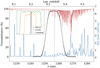 |
Fig. 1. Transmission curve of the NB1257 filter. The black dots show the empirical profile measured in the laboratory to guarantee FWHM = 11 nm and central wavelength λc = 1.257 μm (dashed vertical gray line) at cryogenic temperature. The sky emission of La Palma is overplotted in blue. This sky spectrum was obtained with the EMIR instrument at the GTC. The atmospheric absorption was computed based on the Cerro Paranal Advanced Sky Model and is plotted in red. The filter lies in a wavelength range with minimum sky continuum emission and OH emission of the atmosphere. The inset shows the comparison between the transmission curve of our NB1257 filter (solid black line) and the BB filters WFC3/F125W (solid green line) and J standard (solid orange line) from the Maunakea set of filters. |
The instrumental setup during the observations was composed of two filters: the NB1257 filter, and a broad-band (BB) filter in the J-band region (see Fig. 1 for the respective filter transmissions) as a blocking measure to avoid the light that comes from beyond our intended range. The CIRCE J-band filter is a standard filter from the Maunakea set (Tokunaga et al. 2002). Because our target galaxies are faint, we expected to detect only the emission line without reaching the continuum level in most cases. The transmission curve of the filter has an imperfect box-shaped profile, therefore the final observed emission-line flux will depend on the exact location of the emission line within the wavelength range that is covered by the filter (Villar et al. 2008). In particular, when a bright emission line lies close to the wavelength cutoff, the combination of low transmittance and strong flux is indistinguishable from a fainter emission line that is well centered in the filter.
2.2. CIRCE NB imaging
The final pointing of our CIRCE observations was selected after a visual inspection of the individual WFC3/F140W tiles from the 3D-HST survey in the EGS field. AEGIS-16 is one of the tiles that is covered by the HST, and our CIRCE pointing is centered on it. Based on the feasibility of the observations, the goal was to select a sky region without bright sources, except for a single star that was used for alignment purposes. The bright star in the field (magnitude in the g band of mg = 14.9 mag) was essential to carry out the data reduction (see Sect. 3). The field of view of our CIRCE pointing (3.4 × 3.4 arcmin2, centered at α (J2000) = 14h19m44.67s, δ (J2000) = +52° 53′11.5″) is represented as a blue box in Fig. 2, and the surrounding AEGIS tiles observed by HST/WFC3 are marked with yellow boxes as a reference. The background image displayed in this figure corresponds to the WFC3/F125W filter (CANDELS survey), which encompasses the wavelength coverage of our NB1257 filter.
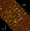 |
Fig. 2. Observation region within the EGS where the AEGIS tiles covered by HST/WFC3 are shown with yellow boxes. The FOV of our CIRCE pointing is marked with a blue box of 3.4′ × 3.4′. Image background: WFC3/F125W from the CANDELS survey. Position: α (J2000) = 14h19m44.67s, δ (J2000) = +52° 53′11.5″. Orientation: North is up, and east is to the left. |
The CIRCE data were obtained between May 2016 and July 2017. They consist of 23 pointings, and because the observations for this program were carried out in service mode, they were conveniently arranged in observing blocks (OBs) of ∼1 h of exposure time. Details of the OBs are given in Table 2. A standard dithering technique (shift + coadd) was used to deal with the cosmetic defects of the detector. Thus, by combining multiple images of a target at slightly different positions on the detector, one can compensate for detector artifacts (such as dead pixels). Each OB consisted of 11 or 12 dithered locations around the central coordinates of the target field, with offsets of a few dozen arcseconds (∼1/10 of the CIRCE FOV). At each particular telescope pointing within the dithering pattern, several consecutive exposures (three or five) were obtained before moving to the next location in that pattern. In turn, each exposure was performed in correlated double sampling (CDS) mode by reading the detector twice, once at the beginning and once at the end of the predefined exposure time. The subtraction of these two readings in CDS mode leads to the scientific image that is commonly referred to as the ramp. The raw FITS images provided by the telescope contain the individual readings carried out at each telescope location within the dithering pattern (where each reading is stored as an independent FITS extension). As an example, for the first OB (see Table 2), the completion of this observing block provided 11 raw FITS files containing six extensions, that is, three exposures of 100 s each. We did not need specific calibration images because no large objects were present in the images. In this case, the science images themselves were used for flat fielding and sky subtraction.
Summary of the observing blocks.
2.3. HST/WFC3 near-IR imaging and ancillary data
The 3D-HST survey provides very deep imaging in a large number of photometric filters. In particular, it includes HST/WFC3 data taken with the F125W, F140W, and F160W filters for ∼41 200 objects over an area of ∼206 arcmin2 within the EGS field. Because very high-z galaxies at z ∼ 9.3 will be dropouts in all photometric bands bluer than J, we used the F125W data as our reference BB image. This comparison should allow us to select targets with a flux excess in the NB1257 filter. The transmission curve of the F125W filter is plotted in green in the inset of Fig. 1, where the narrowness of our NB1257 filter is highlighted over the other filters. The great advantage of the 3D-HST treasury program is the spatially resolved low-resolution spectroscopic data taken by the WFC3/G141 grism (wavelength coverage of 1.1–1.7 μm).
In order to exploit different catalogs that are publicly available, we also gathered the archival data from the Cosmic Assembly Near-infrared Deep Extragalactic Legacy Survey (CANDELS) for the EGS field, which provides robust photometric redshifts and stellar masses inferred from spectral energy distributions (Stefanon et al. 2017).
3. Data reduction
We detail in this section the data reduction procedure that we used to generate the final deep NB image. We used different tools and routines to reduce the NB data, such as Python codes developed by ourselves (code available in GitHub3), some tasks of IRAF (Image Reduction and Analysis Facility4, Tody 1986, 1993), the CLEANEST5 software to interpolate defective pixels, and the IMCOMBINE6 software, a Fortran program to reduce near-IR images. All of this allows us to control the reduction process step by step, as shown in the flowchart in Fig. 3, where the whole data reduction process was subdivided into three main steps:
 |
Fig. 3. Flowchart of the CIRCE data reduction procedure. Because the procedure is complex, we divided it into three steps as explained in detail in the text. Starting from the raw frames provided by the telescope and generating the single images (step 1), and after performing some additional manipulations, we obtain the combined images of each OB (step 2), and finally, the deep NB1257 image (step 3). |
– Step 1: Reduction of each raw image by extracting and combining the different ramps, and generating a single image corresponding to each particular location within the dithering pattern of the considered OB.
– Step 2: Combination of the resulting images from step 1 corresponding to the same OB. This process generates a single combined OB image.
– Step 3: Combination of the resulting images from step 2 corresponding to the valid OBs.
Each of these steps is described in more detail in the following subsections.
3.1. Step 1: Single image at each telescope pointing
As previously explained, the subtraction of consecutive detector readings leads to ramp images of the predefined exposure time. An example of one of these ramps is shown in Fig. 4. Near-IR detectors typically exhibit more cosmetic defects than their optical CCD counterparts, and, as is evident from this figure, the CIRCE detector was not an exception. Two of the 32 detector channels were not useful (vertical columns from 321 to 384 and from 1473 to 1536), while the detector had a non-negligible number of bad pixels, particularly near the borders and in the upper left corner.
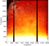 |
Fig. 4. Ramp image taken with the CIRCE detector. Exposure time: 100 s. Size: 2048 × 2048 pixels. The borders of the detector are not useful because of the poor cosmetic. There are many defective pixels and two nonfunctional channels (vertical dark columns located at X coordinates ∼350 and 1500). |
Although we started the observing program requesting OBs with individual integrations of 100 s per ramp (OB0001 to OB0003) and three ramps per telescope pointing (i.e., location within the dithering pattern), we discovered that this strategy was not adequate for our purposes after examining in detail the straightforward combination of the three ramps in each raw frame. Because the GTC did not provide guiding correction for CIRCE exposures, the point spread function (PSF) of the bright star visible in the field of view sometimes appeared slightly elongated after 300 s, which meant that the telescope tracking was not always good enough to prevent the drift of the telescope during the integration at each telescope location. To alleviate this problem, two actions were taken: (1) we modified the observation strategy for the remaining OBs of this program by reducing the exposure time per ramp from 100 to 60 s and by subsequently increasing the number of ramps (exposures at each telescope location) from three to five in each raw frame (to preserve a total exposure time of 300 s at each position within dithering pattern), and (2) we split the individual ramps within each raw frame to measure and apply any potential offset between ramps before their combination. The second action led to the introduction of this step 1 in the reduction procedure.
As graphically described in Fig. 3 (left panel), this step took an individual raw frame as input and generated a single image resulting from the refined combination of the available ramps (three or five). Initially, the individual ramps were extracted separately. Because it was necessary to remove the background level to clearly see even the brightest object in each image, we used as background level for each ramp the corresponding ramp in the next raw frame within the dithering pattern (ramps within the same raw frame cannot be subtracted for this purpose because all of them corresponded to the same telescope pointing).
Because the goal of this reduction step was to detect any potential offset between the different ramps due to the imperfect telescope tracking, we chose the bright star present in the field to apply a 2D cross-correlation technique. Considering the relatively high number of defective pixels in the CIRCE detector, we found it essential to interpolate these defective pixels in order to avoid biased results in the cross-correlation procedure. This cosmetic process was carried out manually using the specialized software CLEANEST to remove bad pixels in an image subregion around the location of the bright star. The measured offsets derived by applying the 2D cross-correlation technique were rounded to integer values. Although these values were rounded to zero for many cases, the offsets amounted up to three pixels in a particular direction for some ramps. In these cases, the offsets were corrected to obtain perfectly aligned ramps. To have an idea of the uncertainties associated with the measured offsets, we repeated this process several times by situating the bright star at different positions within the window of 41 × 41 pixels that we employed when we computed the cross-correlation function. In all cases, the measured errors were always smaller than 1 pixel (i.e., 0.1 arcsec).
After all the ramps within each raw frame were properly aligned, we combined them using the median value for each pixel, which allowed us to reject some defective pixels. However, the offsets were zero in many cases, and therefore this median combination did not remove the majority of the bad pixels.
3.2. Step 2: Combined OB image
By repeating the previously described step 1 for all the individual raw images (11 or 12, depending on the considered OB) of each observing block, we ended up with the same number of single images, one at each location within the dithering pattern. The main objective of step 2 here described (see Fig. 3, middle panel) was to align and combine these individual images to generate a single combined image for each OB. The bulk of this process was carried out using IMCOMBINE, as described below. One of the inputs of this program is the offsets between individual images, but the coordinates of the header were not accurate enough to use them. Therefore, the relative offsets between the single images were obtained by following the same procedure as for computing the offsets between ramps, that is, by using the 2D cross-correlation technique in manually cleaned image subregions of ∼100 × 100 pixels around the two brightest stars (in this case, each single image was now a combination of three or five ramps, which allowed the application of the cross-correlation technique on the second brightest star as well). For each OB, the offsets were always measured relative to the first single image in the sequence, which provided the actual dithering pattern followed by the telescope when carrying out the observations of that particular OB. Although the OB0023 was initially composed of 11 frames because the faint star was barely visible in two single images and the bright star fell in one of the inactive channels of the detector, we discarded these two single images (see Table 2, Col. 2) because it is not possible measuring the corresponding offsets.
In Fig. 5 we overplot the dithering patterns for all the OBs finally used in the generation of the final image with different colors, using the pointing of the first image of OB0001 as a common reference. The program IMCOMBINE, especially written by one of the authors to combine near-IR images, takes as input a list of the single images to be combined, the initial offset determination between them, a bad-pixel mask (facilitated for us by the PI of CIRCE), and a previously computed dark image. In addition, the program is able to compute an object mask, which is initially set to zero and initialized with the detected sources at the end of the execution of the program. In subsequent executions of IMCOMBINE, the object mask was employed and conveniently updated. The different manipulations carried out by this program are listed below.
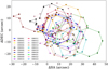 |
Fig. 5. Dither patterns of the 20 OBs used in this analysis plotted with different colors. The offsets were obtained using two stars as reference and refined using the cross-correlation technique. We took the first image of OB0001 as the reference point (0,0). The error bars are too small (smaller than 0.1 arcsec) to be seen in the figure. |
1. Normalize individual (image−dark) frames, dividing by the median of the full image, excluding the already detected objects (none in the first execution of the program, and those detected in step 6 below in subsequent executions), and avoiding also the pixels that are included in the bad-pixel mask.
2. Compute superflat from the mean of the stacking of the normalized images, excluding pixels in the object mask.
3. Compute individual (image−dark)/superflat.
4. Sky subtraction in (image−dark)/superflat: the sky level is computed as the median of the signal in each channel of the CIRCE detector, avoiding pixels included in either the bad-pixel or the object masks.
5. Combine sky-subtracted (image−dark)/superflat frames: for each pixel, the median value of all the pixels in the available frames is computed. Two auxiliary images are also generated, storing the median absolute deviation and the number of pixels from the individual frames employed for each pixel in the final image.
6. Generate the object mask using SExtractor (Bertin & Arnouts 1996). We performed some tests to determine the optimal SExtractor detection parameters that maximized the number of detected objects while minimizing the number of false detections.
The careful examination of each combined OB image revealed that the image background was far from perfect. It exhibited some deviations from zero at intermediate scales. These imperfections were more noticeable at the borders of the combined images, indicating that the bad-pixel mask was not too aggressive (i.e., it did not contain too many bad pixels), which in turn could produce systematic variations in the computation of the superflatfield in these image regions. Instead of dramatically increasing the list of bad pixels, which would have led to a significant loss of the effective field of view in the combined images, we decided to remove the background variations making use of the NEBULISER program that is included in the CASUTools package7. Although initially developed to fit spatially varying nebulosity in images, this software program works very well for modeling varying backgrounds at medium and large scales through the use of a series of iterative sliding median and mean filters that are applied to each axis or to both simultaneously (Irwin 2010). In Fig. 6 we compare the result of applying this correction in one of the combined OB images. It is clear that the good tracking of background variations allows removing a significant amount of the dark structures of the image. This effect is even more pronounced when comparing the result of combining the 20 final OB images before and after applying the nebular filter. Hence, after applying NEBULISER, the image is flatter. This reduces the errors in the photometry in the final NB1257 image.
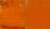 |
Fig. 6. Comparison between a final OB image before (left panel) and after (right panel) applying the nebular filter. Although there are still noisy areas around the borders as a consequence of the dithering and the bad cosmetic of the detector, many dark spots disappear. This flattens the final image and allows us to perform reliable photometry. |
3.3. Step 3: Final NB1257 image
The final step 3 in the data reduction process (see Fig. 3, right panel) consisted of the combination of the final images of each OB obtained after the execution of step 2, with the goal to build the final NB1257 image. Although the initial data set consisted of 23 OBs, just a simple visual inspection of the images corresponding to OB0016, OB0017, and OB0018 revealed that they exhibited an unexpectedly high noise level. We found no reasonable explanation for this, apart from the fact that these three blocks correspond to observations carried out in two consecutive particular nights. It is therefore likely that some problem related to the electronics of the instrument was responsible for it. We performed an exhaustive analysis of the noise of the images to select only the best OBs for the final combination. Further details about the method we followed in this case are provided in Appendix A. Because this analysis revealed what we previously saw by eye, we decided to remove the affected OBs before the final combination (Table 2, Col. 8). The dithering technique makes the good alignment of the individual images crucial for the seeing measurements. The mean seeing during the observations was 0.76 ± 0.14″, and we show in Col. 6 of Table 2 the seeing values of the final image of each OB. The observations were spread over a year, and although there were seeing variations, we demonstrate in Appendix A that in the case of our images, the noise dominates the signal-to-noise ratio (S/N) of the final NB1257 image. For this reason, we decided to use only the OBs that contribute to increasing the S/N of faint sources in the final combination.
After discarding the unusable images, the total exposure time of the remaining 20 OBs amounted to 18.3 h. Before piling up the useful OBs, we discovered that some of them exhibited a non-negligible counter-clockwise rotation of 3 degrees. For the final combination, we therefore made use of the IRAF tasks ROTATE, CCDPROC, and IMCOMBINE, which allowed the rotation correction, the determination of the relative offsets between individual images, the cropping of some noisy image borders, and the final image combination. The last step was to reverse the image in the X direction.
The final deep NB1257 image is shown in Fig. 7 (left panel). Our final image exhibits cosmetic defects, especially at the borders. These are regions with low S/Ns that are located at the edge of the FOV, which are caused by the dithering pattern. Nevertheless, an important fraction of the image is useful for our scientific purposes, although it is worth noting that not all parts of the image were exposed equally, and different depths were reached. This effect is clearly visible in the RMS noise map (Fig. 7, middle panel) where the less noisy region (i.e., the deepest) is found at the center of the image, while the RMS increases significantly at the edges. The RMS noise image was obtained using the photutils.background package of PHOTUTILS8, which provides several tools for detecting and performing photometry of astronomical sources (Bradley et al. 2020). Although the field of view of each CIRCE pointing is 3.4 × 3.4 arcmin2, the combined OB images were trimmed before the final combination since the borders of the images are severally affected by the bad cosmetic of the detector, and the area covered by the final NB1257 image is 2.58 × 2.58 arcmin2. For comparison, and because we chose it as our BB image, we also show in Fig. 7 (right panel) the image taken in this region by the HST with the WFC3/F125W filter.
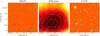 |
Fig. 7. Field of view within the EGS field. The positions of the detections are plotted with open circles: blue for already identified objects at lower redshifts (subsample 1) and gray for sources without an HST counterpart (subsample 2). Left panel: GTC/CIRCE deep image (NB1257 filter) with 18.3 h of exposure time. Middle panel: RMS noise contour map of the NB1257 image in ADU/s. Right panel: HST/WFC3 image (F125W filter) with 25.9 h of exposure time. Orientation: North is up, and east is to the left. Size: 2.6 × 2.6 arcmin2. |
4. Image characterization and source detection
In this section, we describe several steps that are required before the candidate identification. First, we explain the process of PSF matching and flux calibration between the broad and the narrow images. Then, we determine the optimal parameters for the sources extraction, and finally, we study the contamination and detection completeness of the NB1257 image.
4.1. PSF matching and flux calibration
Before the source detection was carried out and the photometry was measured, the NB1257 and F125W images must have the same size and pixel-by-pixel coordinates to ensure that we measured fluxes at the same positions and apertures in both images. First, we used the IRAF task MAGNIFY on the WFC3/F125W HST image to match the pixel step size of the NB1257 image (0.1 ″ pixel−1). Next, we aligned both images using the bright sources of the field as a reference.
We smoothed the WFC3/F125W HST image to the spatial resolution of the NB1257 image (FWHM ∼ 0.8″) using the photutils.psf package (Bradley et al. 2020). In particular, we combined a stack of the brightest but unsaturated isolated stars to build an empirical PSF model for each image. Then, we used the PSFs to generate a matching kernel between both images using the ratio of Fourier transforms. Finally, we carried out a 2D convolution of the HST image and the generated kernel to achieve the PSF matching.
To obtain the zeropoint needed to transform ADU/s of our NB1257 image to AB magnitudes, we took the F125W band as reference, and we assumed that the mean color for the brightest stars was zero, as done in Villar et al. (2008). The flux calibration of the NB1257 image was achieved using the HST/G141 grism spectra (3D-HST survey) of two stars in the field. We computed their synthetic magnitudes using two different Python packages, SYNPHOT9 and PYPHOT10, and we obtained consistent results with the two independent methods (the relative error between the estimated zeropoints was lower than ∼0.0003%).
4.2. Source detection
After matching and calibrating the images, we carried out the source extraction. We ran the Python code SEP11 (Source Extraction and Photometry in Python: Barbary et al. 2015), which is derived from the SExtractor code base (Bertin & Arnouts 1996), on the NB1257 image for the object detection (sep.extract package). We performed some tests to reach the optimal parameters that push the detections as deep as possible while minimizing the false detections. The pixel-by-pixel detection threshold (thresh) was 1.7 × RMS noise image (err). The minimum number of pixels required for an object (minarea) was fixed to match the FWHM area of the PSF and thus set to 50 pixels. The filter treatment (filter_type) was set to matched to ensure a better detection of faint sources in areas of varying noise. The final sample is composed of 97 sources detected in the NB1257 filter, whose coordinates are marked with open circles in Fig. 7. To check the heterogeneous depth of the final image, we compared our RMS image with the one generated using the background estimation of the sep.background package, and no significant difference was found (relative error lower than ∼0.02%).
In an attempt to search for extremely faint objects, we searched all the detections using relaxed constraints. We tested the source extraction using different values of minarea, but values lower than 50 pixels (the smallest area that we can resolve) caused a considerable increase in the number of unreliable detections. For instance, we obtained 157 detected objects when using a value of 40 pixels and 287 objects when minarea was set to 30 pixels. On the other hand, if we varied the thresh parameter to values of 1.5, 1.2, and 1.0, we detected 132, 154, and 246 objects, respectively (with a fixed value of 50 pixels for the minarea). However, this increase in the total number of detected sources was directly reflected in the number of false detections. Therefore, we considered the previous values as the optimal parameters for the source detection, resulting in a total of 97 detected sources.
4.3. Detection completeness and contamination
In order to obtain the depth and quality image assessment, we computed the contamination and completeness levels. First, we used the segmentation map created from SEP to mask the bright sources of the image, and we multiplied the image by −1 to create a negative image in which no objects should be detectable. After running SEP on the negative image with the same set of parameters as were used for the detection in the NB1257 image, we compared the number of objects detected in the negative and the science image as a function of the AB magnitude (calculated with the flux of each object extracted from SEP). This comparison is shown with histograms in Fig. 8 (left panel), where the red bars represent the detections in the negative image and the purple bars the objects detected in the NB1257 image (the positive image). All the objects detected in the negative image are spurious detections. The ratio of these objects and those detected in the positive image in each magnitude bin should represent the contamination levels in the science images. However, the negative image is not fully representative of the NB1257 image because there are magnitude bins where the spurious detections exceed the detections of the science image. We interpreted this as a consequence of the bad cosmetic of the detector. Notwithstanding this fact, we still considered it was useful for determining the magnitudes where we expect more contamination of sources. The number of objects detected in the negative image with magnitudes fainter than 20.4 mag increases considerably, and therefore, we assumed that this magnitude range presents a higher level of contamination. This implies that a non-negligible number of sources detected in this faint magnitude regime are likely spurious-like detections. Despite the small size of our sample, it is clear that there is no contamination for magnitudes brighter than 19.0 mag. Hence, we conclude that the sources detected in this magnitude range are real detections.
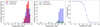 |
Fig. 8. Contamination and completeness levels. Left panel: NB magnitude histogram of objects detected in the negative image (red bars) and in the positive science image (purple bars). Middle panel: histogram with the number of objects detected in the positive science image (purple bars) and the number of them that are already identified objects at lower redshifts (subsample 1, green bars). Right panel: completeness levels as a function of AB magnitude with bins of 0.4 mag. The error bars in the vertical axis represent the 16th and 84th percentiles of the distributions obtained from the simulations. |
We studied the completeness of the final NB1257 image by injecting artificial stars in simulated RMS images and determining the recovered fraction by running SEP. The simulated RMS images were created by measuring the robust standard deviation (see Eq. (A.1)) around each pixel in the NB1257 image (where previously the bright sources were masked) and generating random Gaussian noise with the same standard deviation. Then, we used the STARLIST and MKOBJECTS tasks of IRAF to generate artificial stars and inject them randomly into each image (100 stars/frame, ranging from 17 to 24 mag in bins of 0.4 mag) with a uniform spatial and magnitude distributions. Finally, the completeness levels shown in Fig. 8 (right panel) were derived from the ratio of the numbers of objects detected by SEP at the same positions as the simulated stars and the total number of artificial stars. We repeated this recovering process 20 times for each magnitude bin. The errors in the completeness levels are given as the 16th–84th percentile interval of the distributions obtained from the simulations, which correspond to ±1σ for a Gaussian distribution. The completeness level is 100% at magnitudes lower than 19.0 mag, corresponding to the magnitude range without contamination (see Fig. 8, left panel). Then, it decreases to 50% at 20.8 mag, and at the 5σ limiting magnitude of ∼21.1 mag, the completeness level is 33%. At this stage, we only detected the stars placed in the central region of the image, which corresponds to the deepest region, as shown in the RMS map in Fig. 7 (middle panel). Eventually, the curve reaches zero at 21.6 mag, meaning that beyond this magnitude, we were not able to recover any artificial star in the image.
5. Final sample
Aiming to select candidates to Lyα-emitters at z = 9.34, we built a color-magnitude diagram using the F125W image as our BB image. In addition, we studied our final sample of objects detected by SEP describing the criteria applied for the candidate identification.
First, we categorized the 97 sources detected in our NB1257 into two categories depending on whether they present a counterpart in the F125W image. Subsample 1 contains the sources with an HST counterpart, and subsample 2 includes the sources without a match. After this classification, subsample 1 encompassed 14 objects (four stars and ten galaxies identified in the CANDELS and 3D-HST surveys), while subsample 2 comprised a total of 83 objects. Within subsample 1, we were able to identify ten galaxies in the redshift range z = [0.34 − 1.53]. In addition, eight out of the ten galaxies have an available spectroscopic redshift. We report two possible emission-line sources detected in our NB1257: an OIII[[INLINE280]]4959 emitter at zspec = 1.53, and an OIII[[INLINE282]]5007 emitter at zphot = 1.49 (objects number 50 and 31, respectively). Nevertheless, only spectroscopic follow-up can confirm the latter as a lower redshift contaminant. In Fig. 8 (middle panel) we represent the magnitude histograms of the total sample (purple bars) along with the number of objects belonging to subsample 1 (green bars), corresponding to the objects with HST counterparts. These sources represent a small fraction (∼14%) of the total sample of 97 objects because most of the objects detected in the NB1257 image belong to subsample 2.
We performed an astrometric calibration of our NB1257 image making use of the software WCS tools12 and the public coordinates of the objects in subsample 1. We tested this calibration with the 97 detected objects, finding a median deviation of 0.2″ between our WCS solution and the astrometry of the F125W image. The identification numbers of the whole sample were thus ordered by increasing right ascension.
5.1. Color-magnitude diagram
The key step of the NB technique is to select emission-line candidates by the detection of a flux excess in the NB filter due to their Lyα emission (Murayama et al. 2007; Ouchi et al. 2010; Koyama et al. 2010; Konno et al. 2014). In a first attempt to select candidates, we represent in Fig. 9 the 97 objects detected in the NB1257 image in a color-magnitude diagram. We used the NB1257 image to detect all objects and then measured at the same position (α and δ, J2000) in the WFC3/F125W HST image (our BB image). We compare the magnitude in the F125W filter with the magnitude in our NB1257 filter, distinguishing between the two subsamples with different colors. The magnitudes were defined with a 0.8″ radius aperture, which corresponds to twice the FWHM of the PSF. We also checked the color-magnitude diagram with slightly different aperture sizes, but did not recover new candidates. In this type of diagram, the points around the mean color are distributed asymmetrically. Their dispersion increases with NB magnitude. This dispersion, usually originated from the intrinsic color of each object, for our sample is mainly due to the large uncertainties in the flux measurements of faint sources. In our case, the objects with magnitudes in the NB1257 filter fainter than ∼20.0 mag deviate significantly with respect to the mean color. It is possible that different sensibilities in the two filters cause the asymmetry in the diagram (the flux in the NB1257 filter might be overestimated). Moreover, incorrectly centered apertures in the BB image might generate a systematic effect in the color. We tested this aftermath by measuring the F125W fluxes in the centroid of the sources belonging to subsample 1 (i.e., the sources with a counterpart in the F125W band) and computing the mF125W − mNB1257 color again. The color change is only relevant for object number 50, which is shown with a red arrow in Fig. 9. When we use the position of the NB1257 detections to measure the fluxes in the BB band, we underestimate the F125W fluxes (and thus overestimate the corresponding colors). However, when the offset between the center of the apertures is relatively small (smaller than ∼0.4″), which is the case for most objects, this effect is negligible in the color-magnitude diagram. For the faintest sources alone, the position of the NB1257 detection is significantly different from the centroid of the source measured in the F125W band. Only object 50 exhibits a relevant discrepancy in color (see Fig. 9). We took this outcome into account, but it did not affect the candidate selection in the end.
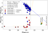 |
Fig. 9. Color-magnitude diagram of the final sample with magnitudes measured within 0.8″ radius apertures. Red symbols indicate the position of subsample 1 (objects with an HST counterpart): filled circles and stars represent the galaxies and stars, respectively. Blue circles represent subsample 2 (objects without HST counterpart). The solid horizontal black line shows the upper limit to the color produced by an emission line. The dotted orange line is the selection curve with a level of significance of nσ = 3.0 (Pascual et al. 2007). The 5σ (1σ) limiting magnitude in the NB1257 (F125W) filter is marked with a vertical dotted gray (diagonal blue) line. The position that the very high-z galaxies EGSY8p7 (Zitrin et al. 2015), EGS-zs8-1 (Oesch et al. 2015), and MACS1149-JD (Hashimoto et al. 2018) would have in our color-magnitude diagram is plotted with an orange, green, and pink triangle respectively. The dashed horizontal gray line marks the mF125W − mNB1257 = 0 reference to guide the eye. The identification number of some objects (discussed in more detail in the text) is provided. The red arrows indicate the color of the sources in subsample 1 using the centroid of the objects in the F125W image instead of the position of the NB1257 detections to measure the BB fluxes. The arrow is discernible only for the faintest source. |
The errors of the NB1257 (F125W) fluxes were calculated by measuring photometry in the NB1257 (F125W) RMS noise image with the same size aperture. The errors for subsample 2 are quite significant, but are almost negligible for subsample 1. The reason is the nondetection in the F125W band. The color that a candidate can have due to an emission line is limited by the ratio of the effective widths of the BB and the NB filter (Pascual et al. 2007). In our color-magnitude diagram, this upper limit (Fig. 9, solid horizontal black line) clearly divides our sample into two groups (red and blue dots), corresponding to our two subsamples. Moreover, most of the sources in subsample 2 follow the diagonal cloud of the 1σ limit of F125W data (dotted blue line). All the sources that are offset from the diagonal trend were identified in the aperture photometry as contaminated by the flux of a nearby object, which would explain their position in the diagram. We expect redder colors as the NB1257 magnitude increases, until the 5σ limiting magnitude of ∼21.1 mag is reached (Fig. 9, vertical dotted gray line). It is worth noting that red colors (i.e., faint BB fluxes with respect to the NB signal) imply large equivalent widths (Villar et al. 2008). The equivalent widths were computed following the approach described in Hayes & Östlin (2006) (see also Pascual et al. 2007). As expected, the estimated EWs of most of the sources belonging to subsample 2 (except for objects 28 and 78) resulted in negative values because the color limit was exceeded. The extended sources of subsample 1 cover a wide range of observed equivalents widths: EWobs ∼ [23–797] Å (with the exception of object 31).
LAEs at z = 9.3 should show a flux excess in the NB1257 with respect to the F125W band. The selection curve defined by Pascual et al. (2007) was employed to identify LAE candidates above the curve (Fig. 9, dotted orange line). The level of significance was set to nσ = 3.0 and the curve was extrapolated using a polynomial fit because the data do not contain enough points to directly calculate the dispersion in all the NB1257 magnitudes intervals. We found two sources in the region of LAE candidates: objects 28 (α = 14h19m41.15s, δ = +52°53′15.9″) and 31 (α = 14h19m41.51s, δ = +52°52′00.2″). Figure 10 shows their stamps in the NB1257 filter and the ACS/F814W and WFC3/F125W HST bands. Moreover, the NB1257 image was smoothed by a median filter for visual purposes because this image highlights the signal better. The position of the NB1257 detection is marked with a black circle (radius of 0.8″). Object 31 has a counterpart in the F125W band, and the position of the NB1257 detection corresponds to the centroid of the source in the BB image with an angular separation smaller than 0.1″, meaning that its color is not affected by a systematic effect due to incorrectly centered apertures (see Fig. 9, its red arrow is too small to be noted). The estimated rest-frame equivalent widths for objects 28 and 31 were EW0 ∼ 45 Å and 204 Å, respectively. This agrees well with the limit (Lyα EW0 ≳ 20 Å) derived from classical LAEs detected with NB filters (Stark 2016; Ouchi et al. 2020). Furthermore, the EW of object 31 is consistent with the results found for the luminous galaxy CR7 (Sobral et al. 2015, 2019) at z ∼ 6.6 (EW0 ∼ 210 Å).
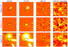 |
Fig. 10. Sample stamp images of objects 28, 31, and 78 in the HST ACS/F814W and WFC3/F125W bands, our NB1257 filter, and a median filtered version of the latter (NB1257 smoothed, computed only for displayed purposes). The 0.8″ radius aperture is plotted with a black circle at the center of the stamp, corresponding to the positions of the detection in the NB1257 image. The sources nearby object 78 are marked with arrows and the 3D-HST identification number. Orientation: North is up, and east is to the left. Size: 7 × 7 arcsec2. |
Object 78 (α = 14h19m49.39s, δ = +52°52′36.2″) is one of the two sources of subsample 2 that are located below the color limit. It shows a slightly NB1257 excess, but not enough to be placed above the selection curve. Although the signal of the object is observed in the NB1257 smoothed stamp, the F814W band reveals that the position of the object does not match the center of any foreground object (see Fig. 10). This is a particular case where the presence of an extremely nearby object led to a failed source detection. This was the reason why object 78 was initially classified into subsample 2. Its color is extremely affected by the presence of nearby sources due to contamination by flux during the aperture photometry. We provide the coordinates and redshifts (photometric and spectroscopic) of the three sources nearby object 78 in Table 3 in order to investigate whether an emission line might affect this measurement. Nonetheless, according to the available redshifts of these galaxies, no emission line lies within the wavelength range covered by our NB1257 filter.
Properties of the galaxies nearby object 78.
By comparison with other studies, we included the expected location of three very high-z galaxies from the literature in our color-magnitude diagram (Fig. 9, triangles). The F125W and NB1257 magnitudes were computed using the published Lyα fluxes and EWs. In particular, we derived the expected colors of the spectroscopically identified galaxies MACS1149-JD at z = 9.1096 (Hashimoto et al. 2018; Hoag et al. 2018; Ouchi et al. 2020; Laporte et al. 2021), EGSY8p7 at z = 8.683 (Zitrin et al. 2015) and EGS-zs8-1 at z = 7.7302 (Oesch et al. 2015). We conclude that all these galaxies, even the two luminous galaxies in the EGS, are beyond the limiting magnitude of this work and therefore would be undetectable in our NB1257 image.
5.2. Final candidate analysis
We decided to conduct a more quantitative analysis based on complementary parameters to verify the robustness of the detections. This allowed us to determine not only possible candidates, but also whether the detections are real or spurious. For this purpose, we took the following complementary criteria into account:
1. The position in the color-magnitude diagram: LAE candidates should be placed above the selection curve and below the color limit.
2. The nondetection in the ACS/F606W and ACS/814W bands: We do not expect z ∼ 9.3 LAEs to be detected in any of the filters blueward of the Lyα line redshifted to 1.257 μm.
3. The counterpart in the WFC3/F160W and IRAC–3.6 μm and 4.5 μm bands: The ultraviolet (UV) continuum from luminous Lyman-break galaxies (LBG) at very high z could be observed in filters redward of the J band (Haiman & Spaans 1999; Chanchaiworawit et al. 2017).
4. The shape of the objects derived from the ellipse parameters extracted from SEP (major semi-axis, minor semi-axis, and position angle): Because very high-z LAEs tend to be compact sources (Pascarelle et al. 1996; Finkelstein et al. 2011; Ouchi et al. 2020), elongated sources are prone to be spurious LAE identifications.
5. The shape of the member pixels of each object in the segmentation map extracted from SEP: For the same reason as before, we are cautious with extended sources that might be generated by noise structures.
6. The position in the RMS noise map: The edges of the NB1257 image are high-noise regions (see Fig. 7, middle panel). Objects detected near the borders are therefore likely spurious detections, unless they are bright sources.
A careful visual inspection of the 97 objects in all the available bands was performed independently by three of the authors. However, we did not select any candidate by the dropout technique. All the sources of the sample either present a counterpart in the bands blueward of the NB1257 band (criterion 2) or do not show a significant signal in any band, including the H and 3.6 μm bands in the red part of the spectrum (criterion 3).
Considering these criteria, we conclude that subsample 1 includes the low-z contaminants of the sample, which are all the objects that were previously detected and identified by other surveys as sources at redshifts lower than z ∼ 9. These sources failed color criterion 2 because all of them are clearly detected in the HST images (see Fig. 7, blue circles). On the other hand, subsample 2 contains the objects that are detected in our NB1257 filter, but not in any other band (see Fig. 7, gray circles). We individually studied these objects, and based on the criteria described above, unfortunately, none of them were reliable. Because they were not detected in the blue bands, they satisfied criterion 2. The lack of signal in the F160W band could be produced by a faint UV continuum, evading criterion 3. They are distributed throughout the image, and some of them are located in the deepest part. However, we searched for compact sources that resembled the appearance of other LAE candidates from the literature, but most of these sources were elongated. Their segmentation maps exhibited a scattered rather than concentrated signal. Above all, as shown in Fig. 9, they did not satisfy the required position in the color-magnitude diagram. We hereby state that their NB1257 flux excess was boosted by the noise. These detections were considered spurious-like sources. This result is the consequence of pushing the objects extraction to the limit in an exhaustive attempt of detecting faint sources.
Focusing specifically on the candidates that were selected by their position in the color-magnitude diagram (objects 28 and 31), we analyzed their nature in further detail. Object 28 was initially classified into subsample 2 because it was not detected in the F125W band (Fig. 10). The F814W and F125W stamps show the offset between the position of the detection and the center of the foreground source. As observed for object 78, the contamination by the flux of an adjacent source explains the position of this object in the color-magnitude diagram. Object 31 belongs to subsample 1 and is placed above the selection curve. It is roughly three magnitudes brighter in the NB1257 filter than the F125W. It is clearly detected in all the available bands, although the nucleus is especially bright in the red bands (F125W and F160W). This object was identified as galaxy CANDELS-ID#13218. Nevertheless, the photometric redshift available for this source is z = 1.49, suggesting that the OIII[[INLINE397]]5007 emission-line might be the cause of its flux excess in the NB1257 filter. In this context, the bright signal observed in the F160W band would be produced by Hα emission. Nonetheless, spectroscopic follow-up would be needed to derive firmer conclusions. Ultimately, the two initial selected candidates were thereby rejected as possible LAEs at z ∼ 9.3.
5.3. Complementary candidates from ancillary data
The study of very high-z galaxies is crucial to provide information on the IGM transparency and to identify ionized bubbles. The EGS field has been intensively studied over the past years, and many LAEs have been detected at z > 7 (Zitrin et al. 2015; Oesch et al. 2015; Roberts-Borsani et al. 2016; Stark et al. 2017), suggesting that the IGM is more transparent in this sky region than in other cosmological fields.
Aiming to give new insight into the IGM transparency in the EGS field, we studied the detectability of the Lyα line by searching for very high-z sources in our CIRCE field. To address this point, we used the CANDELS catalog to identify all objects with a redshift solution within the redshift range covered by our NB1257 filter. The CANDELS catalog does not provide the redshift probability distribution P(z), but different photometric measurements with their corresponding 68% and 95% confidence intervals. Within our CIRCE field, we found only two sources with a median photometric redshift measurement (zphot_med) higher than 8, but none of them within the redshift range covered by our NB1257 filter (z = [9.29–9.38]). These objects are CANDELS-ID#36056 (α = 14h19m40.23s, δ= +52°52′06.57″) with a median photometric redshift of zphot_med = 8.0, and CANDELS-ID#37659 (α = 14h19m39.28s, δ = + 52°53′35.20″) with a value of zphot_med = 9.5. No spectroscopic redshift is available for these sources. Object CANDELS-ID#37659 does not have a counterpart in the 3D-HST catalog (the match is not found within a 1″ radius). However, object CANDELS-ID#36056 corresponds to source 3D-HST-ID#17888, and we found a photometric redshift at a peak probability distribution of zpeak = 2.0467 when using the 3D-HST catalog. Hence, we conclude that CANDELS-ID#36056 is likely an interloper at z ∼ 2. The remaining candidate, CANDELS-ID#37659, was not detected in this work, and the aperture photometry reveals an S/N lower than one in the NB1257 image. Because only one candidate is found at zphot > 8, we were unable to stack the data weighted by the P(z) to investigate the detectability of the Lyα line in the early Universe. Multiple factors play a role here: the small area covered by our survey, the small wavelength range covered by the NB1257 filter, and the very high redshift of the sources we are searching for. Because of these factors, we have not found complementary candidates at z ∼ 9.3 from ancillary data within our CIRCE field.
6. Constraints on the z ∼ 9 Lyα luminosity function
Many studies have searched for LAEs using NB filters designed to detect sources with a strong emission line, and specifically, targeting the Lyα line (Ouchi et al. 2008, 2010; Hibon et al. 2010; Chanchaiworawit et al. 2017). However, typical extremely distant galaxies are usually very faint, which makes the spectroscopic confirmations at very high redshift still scarce (Hu et al. 2017; Matthee et al. 2018; Taylor et al. 2021). In this section, we present the depth reached by this work in both flux and luminosity units. We also compute the comoving volume of the survey and study the effect of the cosmic variance for the z ∼ 9 LAE population. Finally, we place an observational upper limit to the Lyα luminosity function at z ∼ 9, and we derive the number density using the very high redshift Lyα luminosity functions available in the literature thus far.
We first computed the emission-line fluxes of the sample following the procedure specified by Pascual et al. (2007). Assuming all the sources to be at z = 9.34, we derived the corresponding Lyα luminosities (LLyα) from the line fluxes of the sources and the corresponding luminosity distance13, which is 9.6 × 10⁴ Mpc. To estimate them, we adopted apertures of radius 0.8″. Considering our 5σ limiting magnitude, we reached an emission-line flux limit of 2.9 × 10⁻¹⁶ erg s−1 cm−2, which corresponds to a Lyα luminosity of 3 × 1044 erg s−1. Down to this limit, we found no robust LAE candidates consistent with the selection criteria described in Sect. 5.2. Conducting a searching of LAEs at z = 8.8, Matthee et al. (2014) found, with a larger number statistics, luminous candidates with similar Lyα luminosities (LLyα ∼ 1.0 × 1044 erg s−1) than ours, although none of them was spectroscopically confirmed in the end.
6.1. Comoving volume
The total area covered by the NB1257 image is 6.67 arcmin2. Assuming the redshift interval z = [9.29–9.38], defined by the FWHM of our NB1257 filter, this corresponds to a volume13 of 1.1 × 10³ Mpc3. This is an upper limit because the final NB1257 image is not homogeneous in depth (see Fig. 7, middle panel). Furthermore, the transmission curves of the filters present a Gaussian shape instead of a box-shaped profile. This implies that the effective volume of the survey is not a fixed value, but rather depends on the combined continuum plus emission-line flux. Thus, a faint source can be detected only if the emission line lies in the center of the filter, whereas the emission from a bright source may be detected even in the wings. In these circumstances, bright galaxies can be detected in larger volumes than their fainter counterparts. However, because our NB1257 filter is extremely narrow, we do not expect this effect to be especially relevant for our work (a factor ∼1.5 in volume, Δlog  0.2.)
0.2.)
Surveying an area similar to ours (6.25 arcmin2), Willis & Courbin (2005) searched for Lyα emission at z ∼ 9 using the NB technique without success. No LAE at z ∼ 9 was detected by Willis et al. (2008) either. They covered roughly twice the total area and reached a flux limit of 3.7 × 10⁻¹⁸ erg s−1 cm−2. Even with a much larger area (32 400 arcmin2), Matthee et al. (2014) proved that identifying these very high-z galaxies is still a challenge.
6.2. Cosmic variance
Our analysis might be affected by observational uncertainties due to the cosmic large-scale structure. To study this effect, we made use of the publicly available IDL code14 described in Moster et al. (2011) to compute the cosmic variance as a function of the redshift bin, the area covered by the survey, and the stellar mass (M⋆) of the galaxies. Assuming that typical LAEs are low-mass (108 − 9 M⊙) galaxies (Ouchi et al. 2020), we found a relative cosmic variance for galaxies with M⋆ < 109 M⊙ of ∼349%. This high value is consistent with Moster et al. (2011), who already stated that for high-z observations it is essential to cover a wide field to reduce the effect of the cosmic variance. For instance, for the whole EGS (area of 700 arcmin2) and for the same redshift interval, the relative cosmic variance for galaxies with M⋆ < 109 M⊙ is ∼94%. In addition to the small area covered, the geometry of our survey contributes to the high cosmic variance because the ratio of the two observation angles (α1 and α2 in Moster et al. 2011) is one, the maximum. This implies that the typical distance between galaxies is small, favoring their correlation. Considering our total area, a ratio of ∼0.3 in the angular geometry would be needed to decrease the relative cosmic variance by a factor of ∼14%.
6.3. Luminosity function
To better understand the evolution of the LAE population, the evolution of the Lyα LF with redshift must be known. Following the nondetections of our survey, we derived an upper limit on the Lyα luminosity function of log(N(> L)) = −3.0 Mpc−3 and LLyα = 3 × 1044 erg s−1 at z ∼ 9. Among the previous constraints from the literature, it is worth noting the faint detection limits reached by Cuby et al. (2007) and Willis et al. (2008) (LLyα = 1.3 × 1043 erg s−1 and LLyα = 1.0 × 1043 erg s−1, respectively) in spite of the small volumes that were surveyed (∼5 × 10³ Mpc3 and ∼2 × 10³ Mpc3, respectively). On the other hand, Matthee et al. (2014) performed a very wide survey (volume ∼5 × 10⁶ Mpc3), which allowed them to place a tight constraint on the bright end of the LF: log(N(> L)) = −6.7 Mpc−3 and LLyα = 6.3 × 1043 erg s−1. However, they achieved the same depth as Sobral et al. (2009) (although in this case, the volume covered was ∼1 × 10⁶ Mpc3), which was insufficient to detect any robust LAE candidate at very high z. Our exclusion zone is consistent with the previous observations at z ∼ 9. The estimated Lyα luminosities at z = 9.34 of galaxies MACS1149-JD and EGSY8p7 were 4.7 × 1042 erg s−1 and 1.9 × 1043 erg s−1, respectively. EGS-zs8-1 presents the same Lyα flux as EGSY8p7, hence the estimated Lyα luminosity would be the same for both galaxies. As we already mentioned in Sect. 5, these galaxies are beyond the depth reached by our work and, in fact, only the surveys conducted by Cuby et al. (2007) and Willis et al. (2008) were deep enough to be able to realistically detect LAEs with the same luminosity as the luminous galaxies of the EGS. No study performed with an NB filter has yet achieved the Lyα luminosity limit needed to detect faint sources such as MACS1149-JD. Nevertheless, not only the depth, but also the volume that is covered contribute considerably to the probabilities of detecting these young galaxies.
In order to study the space density of galaxies as a function of their luminosity, we made use of the Schechter formalism as described in Schechter (1976),
 (1)
(1)
where L* is the characteristic galaxy luminosity, ϕ* is the number density that provides the normalization, and α is the faint-end slope. The current lack of galaxy detections at z ∼ 9 makes it impossible to derive a Lyα luminosity function at this redshift, which implies that the luminosity distribution of the z ∼ 9 galaxy population remains unknown. Even at lower redshifts (z ∼ 6 − 7), the LFs are mostly obtained by fitting a Schechter function with a fixed α value due to the scarce data of faint sources that hinder the faint-end slope constraint. The Lyα luminosity function at the highest redshift to date is given by Konno et al. (2014) at z = 7.3, with the best-fit Schechter parameters of  = 2.7
= 2.7 × 1042 erg s−1 and ϕ* = 3.7
 × 10−4 Mpc−3 for a fixed α = −1.5. Likewise, we also considered the Lyα luminosity function provided by Itoh et al. (2018), who used the data given by Konno et al. (2014) at z = 7.3 to calculate the best-fit Schechter parameters with a steep slope of α = −2.5 (in good agreement with Morales et al. 2021), obtaining values of
  = 0.55
 × 1043 erg s−1 and ϕ* = 0.94
 × 10−4 Mpc−3. On the other hand, Nilsson et al. (2007) made use of several observed luminosity functions at lower redshift to extrapolate the LF at z = 9.4, obtaining the Schechter parameters of log(L*) = 42.92 ± 0.24 erg s−1, log(ϕ*) = 3.96 ± 0.50 Mpc−3 for a fixed α = −1.5. From these LFs, we can compute the number of galaxies per unit of luminosity and volume. Using our Lyα luminosity limit, the result states that we would not expect any LAE detection within our comoving volume. If we consider the same volume but deeper observations, for instance, the estimated Lyα luminosities of MACS1149-JD and EGSY8p7, the expected number of sources would be 0.02 and 0.00002, respectively, when using the LF provided by Konno et al. (2014). It should be noted that the result is an approximation because this LF is derived from observations at z = 7.3 instead of z = 9.3, which means that we would be assuming the case of no Lyα LF evolution from z = 7.3 to 9.3. Notwithstanding, even though the difference in cosmic time between these redshifts is not significantly large (similar to a sample of z = [0.95 − 1.00]), the timescale corresponds to the epoch when the formation of the first galaxies and the reionization took place, which makes observations at these redshifts crucial for understanding how the Universe evolved. We expect a significant evolution of the Universe during the first stages, especially of the IGM, because the double-reionization scenario of the AMIGA model predicts a first peak of ionization around z ∼ 10 (Manrique et al. 2015; Salvador-Solé et al. 2017). The single-reionization approach, which claims that reionization was a progressive process, also supports this substantial change in ionized hydrogen fraction of the Universe between these redshifts. Using the LF extrapolation at z = 9.4 given by Nilsson et al. (2007) with the same depths as MACS1149-JD and EGSY8p7, the number density increases slightly, obtaining values of 0.06 and 0.002, respectively. These results indicate that both the ongoing and the next surveys need to cover larger fields and reach fainter magnitudes to be able to detect very high-z sources.
The low number of confirmed galaxies at z > 7 suggests that luminous sources at very high z may be scarce and therefore difficult to detect. Recently, Goto et al. (2021) confirmed a decrease in bright LAEs at z > 7 by performing an NB imaging survey with no LAE detections down to LLyα = 1.6 × 1043 erg s−1 in an effective volume of 2 × 10⁶ Mpc3. In addition, the nature of the galaxies causing the reionization remains debated due to the uncertainty of the escape fraction of very high-z sources (Dijkstra et al. 2016; Castellano et al. 2018; Rodríguez Espinosa et al. 2021). Especially around z ∼ 9, it is unclear if the main source of ionizing photons comes from bright galaxies (Robertson et al. 2015) or faint galaxies (Finkelstein et al. 2019). Hence, a larger number of confirmed detections at z ∼ 9 is essential for building a reliable Lyα luminosity function for this redshift.
7. Summary and conclusions
This pilot project aimed to study the feasibility of finding Lyα emitters at very high z using the NB filter designed by the ALBA team. For this purpose, we searched for LAEs in a small region within the EGS field with the near-IR camera CIRCE at the GTC telescope and using a NB filter centered at 1.257 μm. The NB1257 filter was specifically designed and built for this project to target LAEs at z ∼ 9.3 exploiting one of the OH sky lines windows. We performed a careful data reduction process to ensure the best alignment of the frames and to minimize instrumental effects. In addition, we conducted an analysis of the noise level of each individual image to select only the OBs with the best quality for the final combination. Finally, with a total exposure time of 18.3 h, we reached a limiting AB magnitude of ∼21.1 mag in our NB1257 image. A total of 97 objects were detected when the source extraction was made. These sources were placed in a color-magnitude diagram, using the F125W band of HST as our BB image, to identify those with a flux excess in the NB1257 filter. Two objects were selected above our selection curve as initial LAE candidates at z ∼ 9. Then, we described several complementary criteria to confirm the robustness of these initial candidates and to analyze all the detections in more detail. At last, no candidates were found down to a Lyα luminosity of 3 × 1044 erg s−1 by probing a comoving volume of 1.1 × 10³ Mpc3. Nevertheless, we placed an observational constraint of the Lyα luminosity function at z ∼ 9 by deriving upper limits from the absence of detections. The exclusion zone reported in this work is consistent with previous observations at this redshift and with the luminosity functions available so far. From these results, we conclude that the combination of both wider and deeper surveys is essential to detect a first sample of z ∼ 9 LAEs. Notwithstanding, the area covered plays an important role not only in the probability of detection, but also because a large field is required to minimize the effects of the cosmic variance in this population of galaxies. Our short-term purpose is to reuse the NB1257 filter in a future near-IR camera, which will allow us to continue searching for very high-z galaxies applying the method we developed and described in this paper. The main motivation is to detect a sample of LAE candidates for subsequent follow-up spectroscopy. If their z ∼ 9 nature is confirmed, these sources will be used to study the feasibility of the double-reionization scenario predicted by the AMIGA model.
In this observational test, we finally did not reach the reionization epoch, but nonetheless, in the near future, several surveys will continue studying the early Universe. The arrival of a new generation of telescopes, such as the SKA (Mellema et al. 2013; Mangena et al. 2020), the JWST (Finkelstein et al. 2017), or the ELT (Sánchez-Janssen et al. 2020), will provide an unprecedented insight into our knowledge about the first galaxies and Population III galaxies. MOSAIC will be a multi-object spectrograph for the future 39 meters ELT, which will be the largest optical and near-IR ground-based telescope. As shown in Vanzella et al. (2014), owing to the high sensitivity and good spatial resolution of MOSAIC, this instrument will improve the magnitude limits in the continuum reached by the near-IR spectroscopy of the JWST (see also the simulations performed for the ELT by Disseau et al. 2014). Hence, MOSAIC will become an essential instrument in the next years, enabling us to derive the properties of faint galaxies detected by the JWST (Hammer et al. 2021) and tracing the reionization. Many questions currently remain unclear, but probing the cosmic dawn is one of the main science cases of these upcoming facilities.
This software utility was initially developed by Cardiel (1999) as part of the  package, and it is at present available as a stand-alone program. See https://cleanest.readthedocs.io/en/latest/
The comoving volume and the luminosity distance at a given redshift were computed using the astropy.cosmology package.
Acknowledgments
We thank the anonymous referee for the useful feedback that served to improve the original manuscript. This research was supported by the Spanish Ministry of Science and Innovation (MCIN) under the grants AYA2016-75808-R and RTI2018-096188-B-I00. C.C. acknowledges the Universidad Complutense de Madrid and the MCIN for the grant PRE2019-087503 “Personal Investigador Predoctoral en Formación”. The authors thank Stephen Eikenberry, PI of the CIRCE camera, for his help during the preparation of the observations. This work is based on observations made with the Gran Telescopio Canarias (GTC), installed in the Spanish Observatorio del Roque de los Muchachos of the Instituto de Astrofísica de Canarias, on the island of La Palma. The authors also thank the support given by Dr. Antonio Cabrera and the GTC Operations Group staff during the observations at the GTC. This study makes use of data from AEGIS, a multiwavelength sky survey conducted with the Chandra, GALEX, Hubble, Keck, CFHT, MMT, Subaru, Palomar, Spitzer, VLA, and other telescopes and supported in part by the NSF, NASA, and the STFC. This work is based on observations taken by the 3D-HST Treasury Program (GO 12177 and 12328) with the NASA/ESA HST, which is operated by the Association of Universities for Research in Astronomy, Inc., under NASA contract NAS5-26555. This work has been possible thanks to the extensive use of IPython and Jupyter notebooks (Perez & Granger 2007). This research made use of Astropy (http://www.astropy.org), a community-developed core Python package for Astronomy (Astropy Collaboration 2013, 2018).
References
- Astropy Collaboration (Robitaille, T. P., et al.) 2013, A&A, 558, A33 [NASA ADS] [CrossRef] [EDP Sciences] [Google Scholar]
- Astropy Collaboration (Price-Whelan, A. M., et al.) 2018, AJ, 156, 123 [Google Scholar]
- Bacon, R., Accardo, M., Adjali, L., et al. 2010, in Ground-based and Airborne Instrumentation for Astronomy III, eds. I. S. McLean, S. K. Ramsay, & H. Takami, SPIE Conf. Ser., 7735, 773508 [Google Scholar]
- Barbary, K., Boone, K., & Deil, C. 2015, sep: v0.3.0, https://github.com/kbarbary/sep [Google Scholar]
- Beniamini, P., Kumar, P., Ma, X., & Quataert, E. 2021, MNRAS, 502, 5134 [NASA ADS] [CrossRef] [Google Scholar]
- Bertin, E., & Arnouts, S. 1996, A&AS, 117, 393 [NASA ADS] [CrossRef] [EDP Sciences] [Google Scholar]
- Bouwens, R. J., Illingworth, G. D., Oesch, P. A., et al. 2015, ApJ, 811, 140 [NASA ADS] [CrossRef] [Google Scholar]
- Bouwens, R. J., Stefanon, M., Oesch, P. A., et al. 2019, ApJ, 880, 25 [NASA ADS] [CrossRef] [Google Scholar]
- Bradley, L., Sipőcz, B., Robitaille, T., et al. 2020, https://doi.org/10.5281/zenodo.4049061 [Google Scholar]
- Brammer, G. B., van Dokkum, P. G., Franx, M., et al. 2012, ApJS, 200, 13 [Google Scholar]
- Brauneck, U., Gallego, J., Cardiel, N., et al. 2018, SPIE Conf. Ser., 10702, 1070223 [NASA ADS] [Google Scholar]
- Cardiel, N. 1999, Ph.D. Thesis, Univ. Complutense de Madrid [Google Scholar]
- Cardiel, N., Pascual, S., Gallego, J., et al. 2019, in Rectification and Wavelength Calibration of EMIR Spectroscopic Data with Python, eds. P. J. Teuben, M. W. Pound, B. A. Thomas, & E. M. Warner, ASP Conf. Ser., 523, 317 [NASA ADS] [Google Scholar]
- Castellano, M., Pentericci, L., Vanzella, E., et al. 2018, ApJ, 863, L3 [CrossRef] [Google Scholar]
- Cen, R. 2003, ApJ, 591, 12 [NASA ADS] [CrossRef] [Google Scholar]
- Chanchaiworawit, K., Guzmán, R., Rodríguez Espinosa, J. M., et al. 2017, MNRAS, 469, 2646 [NASA ADS] [CrossRef] [Google Scholar]
- Cuby, J. G., Hibon, P., Lidman, C., et al. 2007, A&A, 461, 911 [NASA ADS] [CrossRef] [EDP Sciences] [Google Scholar]
- Davis, M., Guhathakurta, P., Konidaris, N. P., et al. 2007, ApJ, 660, L1 [NASA ADS] [CrossRef] [Google Scholar]
- de La Vieuville, G., Bina, D., Pello, R., et al. 2019, A&A, 628, A3 [NASA ADS] [CrossRef] [EDP Sciences] [Google Scholar]
- Dijkstra, M., Gronke, M., & Venkatesan, A. 2016, ApJ, 828, 71 [Google Scholar]
- Disseau, K., Puech, M., Flores, H., et al. 2014, in Ground-based and Airborne Instrumentation for Astronomy V, eds. S. K. Ramsay, I. S. McLean, & H. Takami, SPIE Conf. Ser., 9147, 914791 [NASA ADS] [Google Scholar]
- Eikenberry, S. S., Charcos, M., Edwards, M. L., et al. 2018, J. Astron. Instrum., 7, 1850002 [CrossRef] [Google Scholar]
- Ellis, R. S. 2008, in Observations of the High Redshift Universe, eds. A. Loeb, A. Ferrara, & R. S. Ellis, 259 [Google Scholar]
- Finkelstein, S. L., Cohen, S. H., Windhorst, R. A., et al. 2011, ApJ, 735, 5 [NASA ADS] [CrossRef] [Google Scholar]
- Finkelstein, S. L., Papovich, C., Ryan, R. E., et al. 2012, ApJ, 758, 93 [NASA ADS] [CrossRef] [Google Scholar]
- Finkelstein, S. L., Dickinson, M., Ferguson, C., et al. 2017, The Cosmic Evolution Early Release Science (CEERS) Survey, JWST Proposal ID 1345. Cycle 0 Early Release Science [Google Scholar]
- Finkelstein, S. L., D’Aloisio, A., Paardekooper, J.-P., et al. 2019, ApJ, 879, 36 [Google Scholar]
- Furlanetto, S. R., & Loeb, A. 2005, ApJ, 634, 1 [NASA ADS] [CrossRef] [Google Scholar]
- Garzón, F. EMIR Team 2016, in EMIR, the NIR MOS and Imager for the GTC, eds. I. Skillen, M. Balcells, & S. Trager, ASP Conf. Ser., 507, 297 [Google Scholar]
- Goto, H., Shimasaku, K., Yamanaka, S., et al. 2021, ApJ, 923, 229 [CrossRef] [Google Scholar]
- Grogin, N. A., Kocevski, D. D., Faber, S. M., et al. 2011, ApJS, 197, 35 [NASA ADS] [CrossRef] [Google Scholar]
- Haiman, Z., & Spaans, M. 1999, ApJ, 518, 138 [NASA ADS] [CrossRef] [Google Scholar]
- Hammer, F., Morris, S., Cuby, J. G., et al. 2021, The Messenger, 182, 33 [NASA ADS] [Google Scholar]
- Hashimoto, T., Laporte, N., Mawatari, K., et al. 2018, Nature, 557, 392 [NASA ADS] [CrossRef] [Google Scholar]
- Hayes, M., & Östlin, G. 2006, A&A, 460, 681 [NASA ADS] [CrossRef] [EDP Sciences] [Google Scholar]
- Hibon, P., Cuby, J. G., Willis, J., et al. 2010, A&A, 515, A97 [NASA ADS] [CrossRef] [EDP Sciences] [Google Scholar]
- Hoag, A., Bradač, M., Brammer, G., et al. 2018, ApJ, 854, 39 [Google Scholar]
- Hu, W., Wang, J., Zheng, Z.-Y., et al. 2017, ApJ, 845, L16 [CrossRef] [Google Scholar]
- Hull, A., Brauneck, U., Gallego, J., et al. 2019, Proc. SPIE, 11180, 1118087 [NASA ADS] [Google Scholar]
- Irwin, M. 2010, UKIRT Newsletter, 26, 14 [Google Scholar]
- Itoh, R., Ouchi, M., Zhang, H., et al. 2018, ApJ, 867, 46 [NASA ADS] [CrossRef] [Google Scholar]
- Ivezic, Z., Connolly, A. J., VanderPlas, J. T., & Gray, A. 2014, Statistics, Data Mining, and Machine Learning in Astronomy: A Practical Python Guide for the Analysis of Survey Data (USA: Princeton University Press) [CrossRef] [Google Scholar]
- Jung, I., Finkelstein, S. L., Dickinson, M., et al. 2020, ApJ, 904, 144 [NASA ADS] [CrossRef] [Google Scholar]
- Koekemoer, A. M., Faber, S. M., Ferguson, H. C., et al. 2011, ApJS, 197, 36 [NASA ADS] [CrossRef] [Google Scholar]
- Konno, A., Ouchi, M., Ono, Y., et al. 2014, ApJ, 797, 16 [Google Scholar]
- Koyama, Y., Kodama, T., Shimasaku, K., et al. 2010, MNRAS, 403, 1611 [NASA ADS] [CrossRef] [Google Scholar]
- Kusakabe, H., Blaizot, J., Garel, T., et al. 2020, A&A, 638, A12 [NASA ADS] [CrossRef] [EDP Sciences] [Google Scholar]
- Laporte, N., Ellis, R. S., Boone, F., et al. 2017, ApJ, 837, L21 [CrossRef] [Google Scholar]
- Laporte, N., Meyer, R. A., Ellis, R. S., et al. 2021, MNRAS, 505, 3336 [NASA ADS] [CrossRef] [Google Scholar]
- Laursen, P., Sommer-Larsen, J., Milvang-Jensen, B., Fynbo, J. P. U., & Razoumov, A. O. 2019, A&A, 627, A84 [NASA ADS] [CrossRef] [EDP Sciences] [Google Scholar]
- Mangena, T., Hassan, S., & Santos, M. G. 2020, MNRAS, 494, 600 [NASA ADS] [CrossRef] [Google Scholar]
- Manrique, A., Salvador-Solé, E., Juan, E., et al. 2015, ApJS, 216, 13 [NASA ADS] [CrossRef] [Google Scholar]
- Maseda, M. V., Bacon, R., Franx, M., et al. 2018, ApJ, 865, L1 [Google Scholar]
- Matthee, J. J. A., Sobral, D., Swinbank, A. M., et al. 2014, MNRAS, 440, 2375 [Google Scholar]
- Matthee, J., Sobral, D., Gronke, M., et al. 2018, A&A, 619, A136 [NASA ADS] [CrossRef] [EDP Sciences] [Google Scholar]
- Mellema, G., Koopmans, L. V. E., Abdalla, F. A., et al. 2013, Exp. Astron., 36, 235 [NASA ADS] [CrossRef] [Google Scholar]
- Momcheva, I. G., Brammer, G. B., van Dokkum, P. G., et al. 2016, ApJS, 225, 27 [Google Scholar]
- Morales, A. M., Mason, C. A., Bruton, S., et al. 2021, ApJ, 919, 120 [CrossRef] [Google Scholar]
- Morishita, T., Stiavelli, M., Trenti, M., et al. 2020, ApJ, 904, 50 [NASA ADS] [CrossRef] [Google Scholar]
- Moster, B. P., Somerville, R. S., Newman, J. A., & Rix, H.-W. 2011, ApJ, 731, 113 [Google Scholar]
- Murayama, T., Taniguchi, Y., Scoville, N. Z., et al. 2007, ApJS, 172, 523 [NASA ADS] [CrossRef] [Google Scholar]
- Newman, J. A., Cooper, M. C., Davis, M., et al. 2013, ApJS, 208, 5 [Google Scholar]
- Nilsson, K. K., Orsi, A., Lacey, C. G., Baugh, C. M., & Thommes, E. 2007, A&A, 474, 385 [NASA ADS] [CrossRef] [EDP Sciences] [Google Scholar]
- Oesch, P. A., van Dokkum, P. G., Illingworth, G. D., et al. 2015, ApJ, 804, L30 [Google Scholar]
- Oesch, P. A., Brammer, G., van Dokkum, P. G., et al. 2016, ApJ, 819, 129 [NASA ADS] [CrossRef] [Google Scholar]
- Ouchi, M. 2019, Saas-Fee Adv. Course, 46, 189 [NASA ADS] [CrossRef] [Google Scholar]
- Ouchi, M., Ono, Y., & Shibuya, T. 2020, ARA&A, 58, 617 [Google Scholar]
- Ouchi, M., Shimasaku, K., Akiyama, M., et al. 2008, ApJS, 176, 301 [Google Scholar]
- Ouchi, M., Shimasaku, K., Furusawa, H., et al. 2010, ApJ, 723, 869 [Google Scholar]
- Pagano, M., & Liu, A. 2021, MNRAS, 508, 1915 [CrossRef] [Google Scholar]
- Pahre, M. A., & Djorgovski, S. G. 1995, ApJ, 449, L1 [NASA ADS] [CrossRef] [Google Scholar]
- Pascarelle, S. M., Windhorst, R. A., Keel, W. C., & Odewahn, S. C. 1996, Nature, 383, 45 [Google Scholar]
- Pascual, S., Gallego, J., & Zamorano, J. 2007, PASP, 119, 30 [Google Scholar]
- Perez, F., & Granger, B. E. 2007, Comput. Sci. Eng., 9, 21 [Google Scholar]
- Planck Collaboration VI. 2020, A&A, 641, A6 [NASA ADS] [CrossRef] [EDP Sciences] [Google Scholar]
- Roberts-Borsani, G. W., Bouwens, R. J., Oesch, P. A., et al. 2016, ApJ, 823, 143 [NASA ADS] [CrossRef] [Google Scholar]
- Robertson, B. E., Ellis, R. S., Dunlop, J. S., McLure, R. J., & Stark, D. P. 2010, Nature, 468, 49 [Google Scholar]
- Robertson, B. E., Furlanetto, S. R., Schneider, E., et al. 2013, ApJ, 768, 71 [Google Scholar]
- Robertson, B. E., Ellis, R. S., Furlanetto, S. R., & Dunlop, J. S. 2015, ApJ, 802, L19 [Google Scholar]
- Rodríguez Espinosa, J. M., Mas-Hesse, J. M., & Calvi, R. 2021, MNRAS, 503, 4242 [CrossRef] [Google Scholar]
- Salvador-Solé, E., Manrique, A., Guzman, R., et al. 2017, ApJ, 834, 49 [Google Scholar]
- Sánchez-Janssen, R., Hammer, F., Morris, S., et al. 2020, SPIE Conf. Ser., 11447, 1144725 [Google Scholar]
- Schechter, P. 1976, ApJ, 203, 297 [Google Scholar]
- Schenker, M. A., Ellis, R. S., Konidaris, N. P., & Stark, D. P. 2014, ApJ, 795, 20 [NASA ADS] [CrossRef] [Google Scholar]
- Shibuya, T., Kashikawa, N., Ota, K., et al. 2012, ApJ, 752, 114 [Google Scholar]
- Skelton, R. E., Whitaker, K. E., Momcheva, I. G., et al. 2014, ApJS, 214, 24 [Google Scholar]
- Sobral, D., Best, P. N., Geach, J. E., et al. 2009, MNRAS, 398, L68 [NASA ADS] [CrossRef] [Google Scholar]
- Sobral, D., Matthee, J., Darvish, B., et al. 2015, ApJ, 808, 139 [Google Scholar]
- Sobral, D., Matthee, J., Brammer, G., et al. 2019, MNRAS, 482, 2422 [Google Scholar]
- Stark, D. P. 2016, ARA&A, 54, 761 [Google Scholar]
- Stark, D. P., Ellis, R. S., Charlot, S., et al. 2017, MNRAS, 464, 469 [NASA ADS] [CrossRef] [Google Scholar]
- Stefanon, M., Yan, H., Mobasher, B., et al. 2017, ApJS, 229, 32 [NASA ADS] [CrossRef] [Google Scholar]
- Sutherland, W., Emerson, J., Dalton, G., et al. 2015, A&A, 575, A25 [NASA ADS] [CrossRef] [EDP Sciences] [Google Scholar]
- Taylor, A. J., Cowie, L. L., Barger, A. J., Hu, E. M., & Songaila, A. 2021, ApJ, 914, 79 [CrossRef] [Google Scholar]
- Tilvi, V., Malhotra, S., Rhoads, J. E., et al. 2020, ApJ, 891, L10 [NASA ADS] [CrossRef] [Google Scholar]
- Tody, D. 1986, in Instrumentation in Astronomy VI, ed. D. L. Crawford, Proc. SPIE, 627, 733 [NASA ADS] [CrossRef] [Google Scholar]
- Tody, D. 1993, in Astronomical Data Analysis Software and Systems II, eds. R. J. Hanisch, R. J. V. Brissenden, & J. Barnes, ASP Conf. Ser., 52, 173 [Google Scholar]
- Tokunaga, A. T., Simons, D. A., & Vacca, W. D. 2002, PASP, 114, 180 [CrossRef] [Google Scholar]
- van Dokkum, P. G., Brammer, G., Fumagalli, M., et al. 2011, ApJ, 743, L15 [NASA ADS] [CrossRef] [Google Scholar]
- Vanzella, E., Fontana, A., Pentericci, L., et al. 2014, A&A, 569, A78 [NASA ADS] [CrossRef] [EDP Sciences] [Google Scholar]
- Villar, V., Gallego, J., Pérez-González, P. G., et al. 2008, ApJ, 677, 169 [NASA ADS] [CrossRef] [Google Scholar]
- Willis, J. P., & Courbin, F. 2005, MNRAS, 357, 1348 [NASA ADS] [CrossRef] [Google Scholar]
- Willis, J. P., Courbin, F., Kneib, J. P., & Minniti, D. 2008, MNRAS, 384, 1039 [NASA ADS] [CrossRef] [Google Scholar]
- Wise, J. H. 2019, ArXiv e-prints [arXiv:1907.06653] [Google Scholar]
- Zitrin, A., Labbé, I., Belli, S., et al. 2015, ApJ, 810, L12 [Google Scholar]
Appendix A: OB noise analysis
By visual inspection, we realized that some combined OB images looked noisier than others. In particular, the images taken on the night of 03 June 2017 showed a strange pattern in the background, possibly due to interference with other electronic devices. We searched for possible temperature variations of the detector that might explain this behavior, but we did not detect any significant variation. However, we further analyzed the quality of all the combined OB images in order to quantify the level of noise and to ensure that only the OBs that increased the S/N of the detection were ultimately employed in the final combination.
As explained in Sect. 2, the combined OB images are the result of combining 11 single images, except for OB0005, OB0021, and OB0023, which were built by combining 12, 12, and 9 exposures, respectively (see Table 2, Col. 2). As a consequence of the dithering technique, each combined OB image presents areas with different depths. The robust standard deviation (hereafter referred to as RobustStd) gives us an idea of the noise in a region. It is defined by the following expression (Ivezic et al. 2014):
 (A.1)
(A.1)
where p25 and p75 are the 25th and 75th percentiles, respectively. The use of this robust estimator facilitated the analysis described in this appendix, avoiding the sensitivity of the traditional standard deviation to outliers. This is important considering the bad cosmetics of the CIRCE detector. We calculated the RobustStd of the distribution of pixels in the different areas of each combined OB image. The RobustStd versus the number of individual exposures (Nexp) employed in the combination is plotted in Fig. A.1 with different colors for each OB. As expected, the RobustStd is higher in the image regions that are covered by single exposures, while its value decreases with increasing number of individual overlapping exposures. This behavior is shared by all the OBs, although the absolute value of the RobustStd at a fixed number of exposures changes.
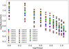 |
Fig. A.1. Robust standard deviation vs the number of exposures employed in the combination for each OB. |
In order to select only the OBs with a high enough quality for the final combination, we sorted out the 23 OBs from lower to higher RobustStd, and combined them by adding one at a time. In the end, we generated a total of 23 combined images. We computed the S/N of a subsample of objects in all these combined images to determine the optimum number of OBs, which we included in the definitive combination. For this purpose, we carried out aperture photometry to extract the fluxes of the selected sources and used the error images generated by the program IMCOMBINE to measure the associated noise (see Sect. 3.2, item 5, for further details). To generate the error image of each possible combination, we added the errors associated with the employed OB images in quadrature. The subsample of objects selected for this analysis was defined taking their location in the image and a magnitude in the NB1257 filter lower than 20.2 mag into account to avoid sources that are dominated by background noise. Figure A.2 shows the variation in S/N when increasingly noisier OBs were added. We started with a single image, the image with less noise (OB0013), and successively added the remaining OB images, sorted by increasing noise. The S/N always improved with more OBs in the combination, except when we included the last 3 OBs. These 3 OBs (OB0016, OB0017, and OB0018) have the highest RobustStd and are therefore noisiest. The S/N clearly decreases away from the maximum, that is, after combination number 20 (marked with a dashed vertical black line). It is worth noting that the brightest star was also included in the subsample and was selected for the analysis, but it is not plotted in Fig. A.2 because its S/N is far higher than the S/N of the other sources (reaching values of S/N ∼ 70), and it never decreased even when the nosiest OBs were included. This implies that this object is so bright that all the other sources of noise are negligible. However, this case is an exception because the final NB1257 image contains no comparable bright source.
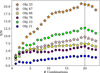 |
Fig. A.2. Variation in S/N according to the number of OBs included in the combination. Filled circles and stars represent the relatively bright galaxies and stars we analyzed, respectively. Different colors stand for different objects. The dashed vertical black line indicates the optimum number of OBs that was used in the final combination. |
Because the inclusion of OB0016, OB0017, and OB0018 did not contribute to an increase in the S/N of the faint sources, we discarded these OBs and decided to combine only the OB images with a value of the log(RobustStd) lower than 0.75. Hence, a total of 20 OBs were used in the final combination that generated the NB1257 image, with an equivalent total exposure time of 18.3 hours.
All Tables
All Figures
|
Fig. 1. Transmission curve of the NB1257 filter. The black dots show the empirical profile measured in the laboratory to guarantee FWHM = 11 nm and central wavelength λc = 1.257 μm (dashed vertical gray line) at cryogenic temperature. The sky emission of La Palma is overplotted in blue. This sky spectrum was obtained with the EMIR instrument at the GTC. The atmospheric absorption was computed based on the Cerro Paranal Advanced Sky Model and is plotted in red. The filter lies in a wavelength range with minimum sky continuum emission and OH emission of the atmosphere. The inset shows the comparison between the transmission curve of our NB1257 filter (solid black line) and the BB filters WFC3/F125W (solid green line) and J standard (solid orange line) from the Maunakea set of filters. |
| In the text | |
|
Fig. 2. Observation region within the EGS where the AEGIS tiles covered by HST/WFC3 are shown with yellow boxes. The FOV of our CIRCE pointing is marked with a blue box of 3.4′ × 3.4′. Image background: WFC3/F125W from the CANDELS survey. Position: α (J2000) = 14h19m44.67s, δ (J2000) = +52° 53′11.5″. Orientation: North is up, and east is to the left. |
| In the text | |
|
Fig. 3. Flowchart of the CIRCE data reduction procedure. Because the procedure is complex, we divided it into three steps as explained in detail in the text. Starting from the raw frames provided by the telescope and generating the single images (step 1), and after performing some additional manipulations, we obtain the combined images of each OB (step 2), and finally, the deep NB1257 image (step 3). |
| In the text | |
|
Fig. 4. Ramp image taken with the CIRCE detector. Exposure time: 100 s. Size: 2048 × 2048 pixels. The borders of the detector are not useful because of the poor cosmetic. There are many defective pixels and two nonfunctional channels (vertical dark columns located at X coordinates ∼350 and 1500). |
| In the text | |
|
Fig. 5. Dither patterns of the 20 OBs used in this analysis plotted with different colors. The offsets were obtained using two stars as reference and refined using the cross-correlation technique. We took the first image of OB0001 as the reference point (0,0). The error bars are too small (smaller than 0.1 arcsec) to be seen in the figure. |
| In the text | |
|
Fig. 6. Comparison between a final OB image before (left panel) and after (right panel) applying the nebular filter. Although there are still noisy areas around the borders as a consequence of the dithering and the bad cosmetic of the detector, many dark spots disappear. This flattens the final image and allows us to perform reliable photometry. |
| In the text | |
|
Fig. 7. Field of view within the EGS field. The positions of the detections are plotted with open circles: blue for already identified objects at lower redshifts (subsample 1) and gray for sources without an HST counterpart (subsample 2). Left panel: GTC/CIRCE deep image (NB1257 filter) with 18.3 h of exposure time. Middle panel: RMS noise contour map of the NB1257 image in ADU/s. Right panel: HST/WFC3 image (F125W filter) with 25.9 h of exposure time. Orientation: North is up, and east is to the left. Size: 2.6 × 2.6 arcmin2. |
| In the text | |
|
Fig. 8. Contamination and completeness levels. Left panel: NB magnitude histogram of objects detected in the negative image (red bars) and in the positive science image (purple bars). Middle panel: histogram with the number of objects detected in the positive science image (purple bars) and the number of them that are already identified objects at lower redshifts (subsample 1, green bars). Right panel: completeness levels as a function of AB magnitude with bins of 0.4 mag. The error bars in the vertical axis represent the 16th and 84th percentiles of the distributions obtained from the simulations. |
| In the text | |
|
Fig. 9. Color-magnitude diagram of the final sample with magnitudes measured within 0.8″ radius apertures. Red symbols indicate the position of subsample 1 (objects with an HST counterpart): filled circles and stars represent the galaxies and stars, respectively. Blue circles represent subsample 2 (objects without HST counterpart). The solid horizontal black line shows the upper limit to the color produced by an emission line. The dotted orange line is the selection curve with a level of significance of nσ = 3.0 (Pascual et al. 2007). The 5σ (1σ) limiting magnitude in the NB1257 (F125W) filter is marked with a vertical dotted gray (diagonal blue) line. The position that the very high-z galaxies EGSY8p7 (Zitrin et al. 2015), EGS-zs8-1 (Oesch et al. 2015), and MACS1149-JD (Hashimoto et al. 2018) would have in our color-magnitude diagram is plotted with an orange, green, and pink triangle respectively. The dashed horizontal gray line marks the mF125W − mNB1257 = 0 reference to guide the eye. The identification number of some objects (discussed in more detail in the text) is provided. The red arrows indicate the color of the sources in subsample 1 using the centroid of the objects in the F125W image instead of the position of the NB1257 detections to measure the BB fluxes. The arrow is discernible only for the faintest source. |
| In the text | |
|
Fig. 10. Sample stamp images of objects 28, 31, and 78 in the HST ACS/F814W and WFC3/F125W bands, our NB1257 filter, and a median filtered version of the latter (NB1257 smoothed, computed only for displayed purposes). The 0.8″ radius aperture is plotted with a black circle at the center of the stamp, corresponding to the positions of the detection in the NB1257 image. The sources nearby object 78 are marked with arrows and the 3D-HST identification number. Orientation: North is up, and east is to the left. Size: 7 × 7 arcsec2. |
| In the text | |
|
Fig. A.1. Robust standard deviation vs the number of exposures employed in the combination for each OB. |
| In the text | |
|
Fig. A.2. Variation in S/N according to the number of OBs included in the combination. Filled circles and stars represent the relatively bright galaxies and stars we analyzed, respectively. Different colors stand for different objects. The dashed vertical black line indicates the optimum number of OBs that was used in the final combination. |
| In the text | |
Current usage metrics show cumulative count of Article Views (full-text article views including HTML views, PDF and ePub downloads, according to the available data) and Abstracts Views on Vision4Press platform.
Data correspond to usage on the plateform after 2015. The current usage metrics is available 48-96 hours after online publication and is updated daily on week days.
Initial download of the metrics may take a while.