| Issue |
A&A
Volume 659, March 2022
|
|
|---|---|---|
| Article Number | A35 | |
| Number of page(s) | 27 | |
| Section | Stellar atmospheres | |
| DOI | https://doi.org/10.1051/0004-6361/202141016 | |
| Published online | 01 March 2022 | |
First detection of a magnetic field in low-luminosity B[e] stars
New scenarios for the nature and evolutionary stages of FS CMa stars★
1
Charles University, Faculty of Mathematics and Physics, Astronomical Institute,
V Holešovičkách 2,
180 00
Praha 8,
Czech Republic
e-mail: This email address is being protected from spambots. You need JavaScript enabled to view it.
2
Department of Physics and Astronomy, University of Victoria,
Victoria,
BC,
V8W 3P2,
Canada
3
Canada-France-Hawaii Telescope Corporation,
65-1238 Mamalahoa Hwy,
Kamuela
HI
96743,
USA
4
Helmholtz-Institut für Strahlen- und Kernphysik, University of Bonn,
Nussallee 14-16,
53115
Bonn,
Germany
5
Institute of Theoretical Physics and Astrophysics, Masaryk University,
611 37 Brno,
Kotlářská 2,
Czech Republic
6
Astronomical Institute of the Academy of Science of the Czech Republic,
Fričova 298,
251 65
Ondřejov,
Czech Republic
7
Department of Physics and Astronomy, University of North Carolina at Greensboro,
Greensboro,
NC
27402,
USA
8
Department of Physics and Astrophysics, University of Delhi,
Delhi
110007,
India
9
Indian Institute of Astrophysics,
Block II, Koramangala,
Bangalore
560034,
India
10
Department of Physics, Montana State University,
PO Box 173840,
Bozeman,
MT
59717–3840,
USA
Received:
7
April
2021
Accepted:
31
December
2021
Abstract
We report the first detection of the magnetic field in a star of FS CMa type, a subgroup of objects characterized by the B[e] phenomenon. The split of magnetically sensitive lines in IRAS 17449+2320 determines the magnetic field modulus of 6.2 ± 0.2 kG. Spectral lines and their variability reveal the presence of a B-type spectrum and a hot continuum source in the visible. The hot source confirms GALEX UV photometry. Because there is a lack of spectral lines for the hot source in the visible, the spectral fitting gives only the lower temperature limit of the hot source, which is 50 000 K, and the upper limit for the B-type star of 11 100 K. The V∕R ratio of the Hα line shows quasiperiodic behavior on timescale of 800 days. We detected a strong red-shifted absorption in the wings of Balmer and O I lines in some of the spectra. The absorption lines of helium and other metals show no, or very small, variations, indicating unusually stable photospheric regions for FS CMa stars. We detected two events of material infall, which were revealed to be discrete absorption components of resonance lines. The discovery of the strong magnetic field together with the Gaia measurements of the proper motion show that the most probable nature of this star is that of a post-merger object created after the binary left its birth cluster. Another possible scenario is a magnetic Ap star around Terminal-Age Main Sequence. On the other hand, the strong magnetic field defies the hypothesis that IRAS 17449+2320 is an extreme classical Be star. Thus, IRAS 17449+2320 provides a pretext for exploring a new explanation of the nature of FS CMa stars or, at least, a group of stars with very similar spectral properties.
Key words: circumstellar matter / stars: emission-line, Be / magnetic fields / stars: evolution / stars: magnetic field / stars: mass-loss
The spectroscopic data of Table 1 are only available at the CDS via anonymous ftp to cdsarc.u-strasbg.fr (130.79.128.5) or via http://cdsarc.u-strasbg.fr/viz-bin/cat/J/A+A/659/A35
© ESO 2022
1 Introduction
IRAS 17449+2320 (BD +23 3183) belongs to a peculiar B-type stellar group known as FS CMa stars, which includes only about sixty members, together with the candidate objects. These stars show the B[e] phenomenon first described by Allen & Swings (1976). Further detailed research and a classification of the B[e] stars was carried out by Lamers et al. (1998), who recognized that the B[e] phenomenon, namely, the presence of forbidden lines and infrared excess, includes stars of different types and at different evolutionary stages. They found the B[e] stars among supergiants, compact planetary nebulae, Herbig Ae/Be stars, and symbiotic stars. However, they were not able to classify about half of stars known at that time. Later, Miroshnichenko (2007) noted that almost all unclassified stars share a set of properties in common and introduced a new group called FS CMa stars. He found the following common signatures: Balmer lines have stronger emission than what is observed in classical Be stars; emission lines of neutral or singly ionized metals from permitted as well as forbidden transitions are also present; weak emission lines of [O III] may be detected; the infrared excess has a peak around 20 μm and sharply decreases toward the longer wavelengths; FS CMa stars are located outside star-forming regions; their temperatures are in the range between 9000 and 30 000 K and luminosity logL∕L⊙ 2.5 and 4.5. The FS CMa group was extended and described in Miroshnichenko et al. (2007, 2011, 2017).
Forbidden lines and infrared excess are indicators of extended circumstellar matter, which complicates the study of the central object. In some cases, we have no information drawn directly from the photosphere. Despite this obstacle, it has nonetheless been found that FS CMa stars are near the Terminal-Age Main Sequence (TAMS) in the Hertzsprung-Russell diagram (Miroshnichenko 2007, 2017; Miroshnichenko et al. 2020a). The presence of circumstellar matter significantly changes the spectrum of the central object. In particular, the UV region may be affected, depending on the angle of view, by the strong absorption of iron group elements, referred to as the so-called “iron curtain”. A great number of absorption lines creates a “false continuum” and may reduce the outgoing UV flux by about an order of magnitude (Korčáková et al. 2019). The energy absorbed in the UV lines is reradiated in the visible and near IR due to the cascade process. Such lines exhibit broad emission wings. The visible spectrum is dominated by very strong emission in the Hα line. The Hα line may be as much as a hundred times brighter than the continuum in some cases. The strongest forbidden lines are [O I] λλ 6300, and 6364 Å, which are always present. Usually [S II] λλ 6716, 6731 Å doublet is detected and in some objects also the doublet of [N II] λλ 6548, 6583 Å. Resonance lines, Na I D1, D2, and Ca II H, and K lines, show a broad emission. The He lines and permitted metal lines may be seen in the emission as well as in the absorption. They usually show rapid night-to-night variability with extreme changes of the line profile from the pure absorption to the P-Cygni profile, inverse P-Cygni profile, pureemission, or absorption with the emission wings (HD 50138, Pogodin 1997; MWC 342, Kučerová et al. 2013).
Currently, there is sufficient spectroscopic and photometric data for some FS CMa stars to search for variability from hours to decades (MWC 623, Polster et al. 2012; MWC 342, Kučerová et al. 2013; MWC 728, Miroshnichenko et al. 2015; HD 50138, Jeřábková et al. 2016; HD 85567, Khokhlov et al. 2017; AS 386, Khokhlov et al. 2018; 3 Pup, Miroshnichenko et al. 2020a). Other studies are based on short observation runs. It was found that spectral lines of most stars show variability at different timescales. Permitted absorption lines of He and metals show usually night-to-night variability, while forbidden emission lines show changes on timescales of months or years. The periodicity of the Hα line has been found on the order of several weeks to years. The best studied photometric periodicity is for MWC 342 (Shevchenko et al. 1993; Mel’Nikov 1997; Chkhikvadze et al. 2002). It shows a short period between 14 and 16 days, with a longer one around 40 and 120 days. The latter has not been found in every season, even if the data would be sufficient to show it. The change of the period from season to season is likely to be a real effect. Here, we note that the scale of the variability ought to be considered, rather than the regular periodicity. On the other hand, a short period of around 27.5 d connected with the orbital motion of the binary has been found for MWC 728 (Miroshnichenko et al. 2015).
The variability of the line profiles reveals that several physical phenomena play an important role in the envelopes of FS CMa stars. The constant outflow of material is accompanied by the appearance of expanding layers (in MWC 342, Kučerová et al. 2013) that may even slow down. The variable shell structure was proven interferometrically by Kluska et al. (2016). Moreover, the episodic material ejecta or cause infall are observable in the resonance lines as discrete absorption components (Korčáková et al., in prep.). Inhomogenities in a rotating disk were discovered in HD 50138 (Jeřábková et al. 2016).
There have been several attempts to measure the mass-loss rate (Ṁ) in FS CMa stars: HD 87643 (de Freitas Pacheco et al. 1982), AS 78 (Miroshnichenko et al. 2000), and IRAS 00470+6429 (Carciofi et al. 2010). The measured values are in the range of 2.5 × 10⁻⁷ to 1.5 × 10⁻⁶ M⊙ yr−1. In particular, de Freitas Pacheco et al. (1982) noted that such a large mass loss cannot be reached by the radiatively driven wind of the central star. This finding is taken as the strongest argument in support of the binarity of FS CMa stars. The large amount of circumstellar matter is naturally explained in this case as resulting from prior or current mass transfer events. A detailed discussion of binarity is presented by Miroshnichenko & Zharikov (2015); Polster et al. (2018); Miroshnichenko et al. (2020b). Indeed, the periodicity, which is interpreted as the orbital motion, was found in a significant stellar sample. To support the binary hypothesis, there are a few examples among FS CMa stars which display a composite spectrum: these are the hot B-type as well as late, usually K-type components. This may be taken as a definitive proof of binarity. However, we are dealing with stars surrounded by a huge amount of circumstellar matter forming the geometrically thick disk and, thus, the interpretation is not so straightforward in this case. The K-type spectrum may be formed through the disk, which behaves as a pseudoatmosphere. The analysis and modeling of the Hα bisector variability of MWC 623 (Polster et al. 2018) favors the radiative transfer effect through the circumstellar disk. The result of this modeling is supported by the polarimetric observations of Zickgraf & Schulte-Ladbeck (1989), which indicates an edge-on view. Up to now, no straight spectral disentangling of any FS CMa star has been successful. The binarity of most (if not every) FS CMa star is a realistic hypothesis because it has been found that most hot stars are indeed part of binaries or multiple systems. A more difficult question to tackle is how the binarity is connected with the observed properties of FS CMa stars.
At this point, we reach back to the three mass-loss rate calculations of de Freitas Pacheco et al. (1982), Miroshnichenko et al. (2000), and Carciofi et al. (2010). There is a serious hidden problem, as every technique is slightly different, but the common factor is the assumption of a smoothly accelerated wind, according to the β velocity law or similar. When these calculations were performed, there were no extended observation campaigns and the authors had no information about the velocity field structure in the envelopes. We now know that the expanding layers may be decelerated (Kučerová et al. 2013). The accumulation of the matter around a star leads to an overestimation of the Ṁ using the smoothly accelerated velocity law. Therefore the real Ṁ may be at least an order of magnitude smaller. Moreover, all three stars are massive FS CMa stars, namely, the radiation pressure is larger than in other members of the group. The inappropriate usage of the velocity law leads us to discard the strongest argument for the binarity of FS CMa stars. Evidence against the binary hypothesis also comes from the interferometric observationsof Kluska et al. (2016). The observations are better described by the model of a disk with a spot rather than by a companion star.
All observed phenomena fit merger, or post-merger, objects. We discuss the pro and con arguments in the Sect. 6.6. The first observation, which points to this hypothesis published de la Fuente et al. (2015). They found two FS CMa stars in the central parts of two clusters.
Our first spectrum of IRAS 17449+2320 indicated that this star may play an important role in revealing the nature of the FS CMa stars. We started the observation campaign at the Ondřejov observatory, which was later extended at other observatories. The results of these data and older archival data are presented in this paper.
2 Observations, data reduction, and the line identification
Observations and data reduction
We were able to collect data from 2005 to 2019 from eight observatories: Canada France Hawaii Telescope, Hawai, USA (CFHT); Apache Point Observatory, New Mexico, USA (APO); Himalayan Chandra Telescope, Leh-Ladakh, India (HCT); Observatorio Astronomico Nacional San Pedro Martir, Baja California, Mexico (SPM); Tien-Shan Astronomical Observatory, Almaty, Kazakhstan (TSAO); Ondřejov Observatory, Czech Republic (OO); Three College Observatory, North Carolina, USA (TCO), and Bellavista Obs. L, Italy (BO). The diameter of the primary mirrors of these telescopes and resolving powers of the individual spectrographs are summarized in Table 1.
The data1 are reduced in IRAF2 using IRAF’s standard procedures, only SPMO data are without the flat field correction. The SPMO and OO spectra are readout without the optimal extraction and the program dcr (Pych 2004) is applied to OO data to remove cosmic rays. The detailed information of the spectra are in Table B.2.
Parameters of the spectrographs used.
Line identifications
The FS CMa stars have complicated spectra. The spectrum may exhibit lines from a hot and a cool component as well as those formed in the circumstellar medium. Accurate line identification and position determinations are crucial for analysis and modeling. Therefore, we decided to do the line identification manually following the lines from multiplets. We present the list of identified lines in the Appendix B.3. We also plotted parts of the spectrum with He I lines (Fig. A.4), which are important for determination of the spectral type because the spectrum shows signatures of a late B- or early A-type star. Besides the strong Balmer and Pashen hydrogen lines and weak He I lines, we found lines of C I, N I, O I, Na I, Mg I, Mg II, Si I, Si II, Ca I, Ca II, Ti II, Cr II, Mn I, Fe I, and Fe II. All the metal lines are in the absorption, with the exception of the [O I] λλ 5577, 6300, and 6364 Å lines and very weak autoionization O I lines at 4355−4356 Å.
3 Spectral properties
The most distinctive feature in the spectrum of IRAS 17449+2320 is the Hα line. Its intensity, reaching values from five to ten times the continuum level, along with the line profile, showing the absorption wings, as well as the V∕R variability indicate that we are dealing with a very special object. The forbidden lines are relatively weak, and we have been able to detect only the forbidden lines of neutral oxygen 5577 Å, 6300, and 6364 Å.
The star is very bright in the UV region compared to a classical Be star (see Sect. 3.1). The UV radiation affects the properties of the spectral lines in the circumstellar region. The lines, which are radiatively connected with the resonance lines, show broad emission wings over the absorption core. However, this non-LTE effect is probably not as strong in IRAS 17449+2320 as it is in other FS CMa stars (Korčáková et al., in prep.). This kind of a line profile is detected only in a few spectral lines. Therefore, we can expect no (or a very weak) iron curtain in the UV region of its spectrum. The high energy of photons also allows for the creation of autoionization lines, which we were able to detect in neutral oxygen as very weak emission and absorption lines. However, we found no Raman lines.
The spectrum is contaminated by interstellar absorption in the resonance lines Na I D1, D2, Ca II H, and K, as well as diffuse interstellar bands (DIBs). The strongest DIB is at 6614 Å. Two other bands, 5780, and 5797 Å, have almost the same intensity. Following the DIB’s families (Galazutdinov et al. 2000; Wszolek 2006), we also identified DIBs at 6196 and 6379 Å.
GALEX data.
3.1 UV radiation
The information about the UV region is limited to data from the GALEX mission. Table 2 summarizes the only observation for IRAS 17449+2320. We used the classical Cardelli’s law (Cardelli et al. 1989) for the dereddening with the parameter Rv =3.1. The GALEX catalog gives E(B − V) = 0.083, which is based on the map of Schlegel et al. (1998). We take the limiting values of E(B − V) as 0.04 and 0.083 corresponding to the spectral types A0 and B9 (see Sect. 6.2 for details), and the intrinsic brightness is in the range 12.2−11.9 mag for FUV, and 12.1−11.7 mag for NUV GALEX bands.
Based on the Gaia parallax (Table 5) the absolute brightness in NUV is between 2.7 and 2.4 mag. This value can be compared with that of a classical Be star, which was observed by GALEX. One of such stars with similar parameters (Teff;Gaia, B9IVn) is 2 Cet. According to the Gaia DR3 parallax and GALEX E(B − V) index, its absolute brightness in the NUV filter is 4.45 mag. If we take the maximum E(B − V) = 0.083 to obtain the upper limit for the NUV brightness of 2 Cep, we obtain the value of 3.9 mag. We note that Be stars were not usually observed in the FUV band. The uncertainties in observation can not explain such a huge difference and IRAS 17449+2320 does have an UV excess compared to the single star without a magnetic field. As we show in the next sections, this UV excess plays an important role in spectrum formation as well as the determination of the stellar parameters.
3.2 Hydrogen lines
The Balmer series lines that were detected are very strong (see Figs. 2, or A.6). We found 17 Balmer lines (Apache Point Observatory, 2016/06/16). The higher members of the series are found fully in the absorption. The first line where a weak emission component appears is Hθ. The emission is shifted bluewards by ~80 km s−1 from the center of the line. The lower the member of the series, the emission is stronger and broader. This behavior, connected with the line formation, is seen in other hot emission-line stars. Beginning about Hδ the central emission becomes more complicated (see Figs. 2, or A.6). The emission in the Hα line reaches about 5–10 x the continuum level. The double-peaked asymmetric emission overlaps the broad absorption wings. The line shows strong V∕R variations (Sect. 4).
Our optical spectra contain the Paschen series lines starting from the Pa ϵ. The latter shows a broad absorption component with a very narrow and strong central emission. The higher the member of the series, the stronger the emission relative to the absorption (see Fig. A.7). The lines from the 18th level are seen fully in emission. We were able to find the line from the 28th level. This sets an upper limit of the electron density at  and of the turbulent velocity at ~ 130 km s−1 (Inglis & Teller 1939; Nissen 1954).
3.3 Helium lines
He lines are represented by relatively strong triplet states (4026, 4471, 4713, and 5876 Å) and weak singlet states (4922, 5016, and 6678 Å), as shown in Fig. A.4. The line 6678 Å shows strong emission wings that are also detectable in 5876 Å line. These two are the only He I lines showing a variability. The other He I lines are seen purely in absorption and are remarkably stable (Fig. A.5). This is the opposite behavior to what is generally observed in other FS CMa stars. Typically, the absorption lines show rapid night-to-night changes, especially He I lines. The line shape may show changes from pure absorption to the P Cygni profile, inverse P Cygni profile, or emission wings or even pure emission.
3.4 Oxygen lines
We detected only the spectral lines of neutral oxygen in the spectrum of IRAS 17449+2320. The strongest are the triplet at 7772, 7774, and 7775 Å and the line at 8446 Å. The triplet shows a wide emission overlapped by very strong and relatively sharp absorption of the individual components. All three lines are Zeeman-split. The 8446 Å line is also in emission with a very narrow and deep absorption component, which in some spectra, reaches intensities that are below the continuum level.
There is also a strong [O I] doublet at λλ 6300, 6364 Å. Both lines are purely in emission and symmetric. Our best spectrum, which has the highest resolution and highest signal-to-noise ratio (S/N) (CFHT 2017-08-14), shows a hint of a very low split blue-shifted emission in the 6364 Å line. Unfortunately, it is impossible to confirm this suggestion on the 6300 Å line because of a contamination with telluric lines. The position of the [O I] doublet does not vary. We found an average value of − 16± 2 km s−1, which is consistent with the measurement of Aret et al. (2016). This allows us to use the radial velocities (RVs) of the [O I] as a reference system value. There is another forbidden line from the same deexcitation cycle (Fig. A.9) at 5577 Å.
Other lines are weak and observed in absorption (Table B.3) with the exception of a weak broad emission formed by the semiforbidden lines in 4355–4356 Å with upper levels above the ionization threshold. Other oxygen autoionization lines present in the spectrum have been found at 3952, 4918, 5573, and 7157 Å.
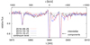 |
Fig. 1 Discrete components of the resonance lines. The events were captured on the SPM spectra on 2013-10-16, following the spectrum over five days, and on 2018-09-25. |
3.5 Resonance lines
Only two resonance doublets, Na I D1, D2, and Ca II H, and K lines, have been detected in the wavelength range from about 3700 to 10 000 Å. The lines always show a broad emission (± 100 km s−1) overlapped by interstellar components. In our spectra, we were able to detect two events of the material ejecta or infall revealing itself as discrete absorption components of these resonance lines (2013-10-16 and 2018-09-25, Fig. 1). The red absorption at 2013-10-16 is shifted about 85 km s−1 relative to the system velocity determined by [O I] lines. Five days later, the absorption was significantly shallower and at the position around 130 km s−1 also redward. This acceleration of the material implies the material infall rather than ejection.
The resonance Li I doublet at 6708 Å deserves a special note, although we were unable to detect it in any of our spectra. Li I lines have been detected in about half of the FS CMa stars (Korčáková et al. 2020). Their presence has been considered a proof of binarity (e.g., Miroshnichenko et al. 2015) because of the low ionization potential of Li I. However, some signatures of these lines can be interpreted as having been formed in the circumstellar disk. The lack of Li I resonance lines may therefore point to the near pole-on orientation. However, this hypothesis has to be taken with caution. The lack of Li I resonance lines may be explained in different ways, especially the optical depth along the line-of-sight is crucial here. Nevertheless, the possibility that we see the system almost pole-on should be taken into account.
4 Variability
4.1 Appearence of a red absorption
We found a very atypical behavior in the spectral lines of IRAS 17449+2320. Occasionally, very strong red-shifted absorption appeared in all the Balmer lines and in the O I triplet 7772, 7774, and 7775 Å. The O I 8446 Å line also shows a slight difference in the red wing. Only minor changes can be seen in the center of the Paschen series. The shape of other spectral lines remains unchanged. We show the C I and N I multiplet in Fig. 2 to demonstrate that even if the shape of the line profile does not change, the intensity does change. This indicates the variability in the stellar continuum. The influence of the continuum intensity is different in different parts of the spectrum. The spectrum with the red-shifted absorption of the Hα and O I lines shows deeper metal lines at longer wavelengths from ~6300 Å, while shallower at shorter wavelengths from this limit.
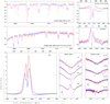 |
Fig. 2 Comparison of the selected parts of the spectra for phases showing the red-shifted absorption (CFHT 2012-02-09, blue lines) and a regular spectrum (CFHT 2006-06-08, red lines). The spectra are corrected on system velocity determined based on the position of [O I] lines. The area with C I multiplet is contaminated by the atmospheric lines. |
4.2 Variability of Balmer lines
Higher members of the Balmer series are variable on time scale of hours; however, only their central emission region up to approximately ± 500 km s−1) varies. The absorption wings remain stable for years, as we show in Figs. 2 and 3. The strong variability is shown in the ratio of the intensity of the violet and red peaks of the Hα line (V∕R, Fig. 4). The data show smooth, almost periodic behavior, with many data points occuring when the violet peak is greater then the red peak. We used a publicly available tool PGRAM on NASA’s web page3 because it isbased on the Lomb-Scargle method (Press & Teukolsky 1988) and, therefore, it is equipped to deal with data that are not equally spaced. The period is determined to be 798 days (Fig. 4, bottom panel). We do not add the error to the result, because this number can not be consider as a regular period, but, rather, as “some scale of the variability”. Figure 4 shows a quasiperiodic tendency rather than a regular one. This behavior is typical for all FS CMa stars (Korčáková et al., in prep.). The ~800 d “period” describes the difference between two well-defined minima.
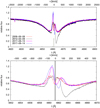 |
Fig. 3 Selected Hβ line profiles from CFHT. Upper panel: remarkably stable wings lasting more than decade, while bottom panel: variable core. The grey arrow on the upper panel and grey vertical line on the bottom panel denote the system velocity position. |
4.3 Radial velocities of SiII lines
To study the RVs, we chose the Si II line 6347 Å as the best tracer. This line is present in every one of our data sets, and it is always in absorption on the spectra of IRAS 17449+2320; moreover, it is narrow and symmetric. On the other hand, it shows Zeeman-splitting in the high-resolution spectra. Unfortunately, we do not have sufficient temporal covering for sufficiently strong magnetic null lines. We measured the RVs using the script from Polster et al. (2012). The value of RVs was determined by automatic line-mirroring using the least square method. The error of the method contains not only the S/N but also effects of possible slight asymmetries or water contamination. The measurements are subject to human control, which allows us to reject unsatisfactory spectra. The Lomg-Scargle method, the box-fitting least-squares method, as well as the Plavchan et al. (2008) method implemented in PGRAM all showed no distinctive peak. Nevertheless, we used the most significant peaks to construct the phase diagram using PHOEBE (eclipsing binary modeling software Prša & Zwitter 2005; Prša et al. 2016; Horvat et al. 2018). All obtained solutions were too affected by the measurement errors and they were very likely unrealistic.
On the other hand, the scatter of Ondřejov data is larger than the error of the individual measurements, suggesting a more complex behavior. Taking into account a very strong magnetic field, Si II is probably concentrated in some spots at the surface (Silvester et al. 2014). Unfortunately, our data quality and temporal covering are not sufficient to reveal the full nature of this behavior.
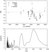 |
Fig. 4 V∕R changes of the Hα line and its periodogram. The horizontal line in the upper panel shows the V∕R = 1 level. Most FS CMa stars have V∕R ratios belowthis line. |
5 Analysis
5.1 Non-LTE effects
The central star is the most important source for the determination of the temperature of the circumstellar matter leading to the presence of neutral and singly ionized metals. In addition, the source of the strong UV radiation also affects the level population.
The UV radiation excites the resonance lines, causing multiple scattering in the circumstellar region. In that situation, the coincidence of the wavelength of individual lines of different elements starts to play an important role. Moreover, the velocity gradient in the photosphere and the circumstellar region do not reach high values, features that support this type of interaction. One of the most important factors is the connection of the population of the hydrogen and oxygen levels through the radiation at Lβ and O I resonance line at 1026 Å. The downward cascade creates emission in the 8446 Å line, emission in the forbidden line at 5577 Å, and the forbidden doublet λλ 6300, 6364 Å. As a consequence, the variability of the Hα and [O I] λλ 6300, 6364 Å lines show the same behavior. A similar situation was found in another FS CMa star, HD 50138 (Jeřábková et al. 2016). This effect has to be taken into account in the analysis of the temporal behavior of IRAS 17449+2320. These conditions allow the creation of autoionization lines. We found weak emission line at 4355 Å and weak absorption lines 3952, 4918, 5573, and 7157 Å. In addition, UV radiation can also form the emission wings, which is the case of the strongest C I lines (Fig. A.1), two N I lines (Fig. A.2), and He I 6678 Å.
We find that Fe I and especially Fe II lines play an important role. A huge number of spectral lines coincide very frequently with lines of other elements. Therefore, the UV pumping of iron lines is very strong. The followup cascades create the emission wings of iron lines. The UV absorption of iron group elements is very strong in FS CMa stars leading to the creation of so called “iron curtain” (Korčáková et al. 2019). However, this effect is not so strong in IRAS 17449+2320 because there are no iron lines fully in emission and only a few of them, which are directly connected with the UV transitions, showing emission wings (Fe II λλ 4923.92, 5018.44, 5169.03 Å).
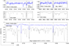 |
Fig. 5 Comparison of selected Fe I and Mg I lines of IRAS 17447+2320 and the Ap star HD 51684 (F0p) with the value of the mean magnetic field modulus: 6 027 ± 50 G (Mathys 2017). |
5.2 Magnetic field
IRAS 17447+2320 shows a clear Zeeman splitting of metallic lines of C I, N I, O I, Mg I, Ti II, Fe I, and Fe II, which makes it possible for application in the case of a straightforward measurement of the magnetic field. We also found Zeeman splitting in the lines of Cr I (4254.35 Å), Cr II (λλ 4242.38, 4252.62, 4558.650, 4565.740, 4836.22, 5237.32185 Å), and Ce II (λλ 4770.91, 5045.12 Å), however, these lines are weak and noisy in our spectra leading to large errors in the magnetic field determination. To guess the size of the magnetic field, we compare the spectrum of IRAS 17447+2320 with that of the Ap star HD 51684 (Fig. 5), which has a mean magnetic field modulus of 6 027 ± 50 G (Mathys 2017), and the Am star o Peg (Fig. A.8), with a magnetic field of about 2 kG (Mathys & Lanz 1990).
We measure the separation of the Zeeman components using a Gaussian profile fitting in IRAF task splot on the CFHT spectrum taken on 2017 August 13. The results are summarized in Table 3. The error is only a formal error of the fit. The corresponding value of the mean magnetic field modulus |B | in G is calculatedbased on (e.g., Adelman 1974):
 (1)
(1)
Here, Δλ in Å is the value of the Zeeman shift, namely, half of the separation of the Zeeman components for doublets, geff is the effective Landé factor, and λ0 is the laboratory wavelength of the line in Å without the magnetic field presence.
The number of Fe II lines with a large split and wide wavelength range is appropriate for a study of the radial gradient of the magnetic field based on the different line formation regions of individual lines. Indeed, the data show a slightly decreasing value of |B | with increasing energy of the lower level (Fig. A.3) with increasing wavelength. However, this guess has to be examined on a larger sample of high quality data to suppress the measurement errors. Currently, a more reasonable value is the arithmetic average of the data, which is 6.2 ± 0.2 kG. We show the value of the mean magnetic field modulus for two other epochs for which we have lower S/N spectra in the Table B.1.
5.3 Stellar parameters
We used for the spectral fitting the code PYTERPOL4 written by J. Nemravová (Nemravová et al. 2016). We used the synthetic grids OSTAR (Lanz & Hubeny 2003), BSTAR (Lanz & Hubeny 2007), POLLUX database (Palacios et al. 2010), ATLAS12 (Kurucz 2005), and AMBRE (de Laverny et al. 2012). Even if the code works well, the fitting of IRAS 17449+2320 spectra is not straightforward. The first complication arises from the presence of the magnetic field. Most spectral lines are split or deformed. The magnetically null lines, usually used for the accurate spectral type determination, are too weak or missing in this star. This leads us to choose only a few intervals with narrow spectral lines (Fig. A.10). It was also necessary to avoid the contamination of the continuum by the circumstellar matter in the IR region. Therefore, we used only the part of the spectra up to 5318 Å. However, more serious problem is caused by the presence of the hot continuum. The strong UV radiation (Sect. 3.1), variability (Sect. 4.1), and the presence of autoionization lines (Sect. 2) reveal this additional radiation. We did not detect spectral lines from this source, but a strong continuum changes the line intensities significantly from the short- to the long-wavelength region. As the source is only the continuum in our region from near UV to near IR, an accurate determination of its temperature and SED in the relative spectra is not possible.
We obtained the best (Table 4 and Fig. A.10) fitting of a binary with a hot and cold component with the solar metalicity. The temperature of the secondary is about 51 000 K and its rotation velocity reaches the value of 800 km s−1. Such a huge value of the rotation velocity means that there are no detectable spectral lines of the hot star in the fitted regions. Since we aredealing with a star with very strong magnetic field surrounded by the circumstellar material, it would be better to talk rather about the hot continuum source than about the secondary component. As we detected the signatures of the material infall (Sect. 3.5), we should take into account also the possibility that infalling material creates a hot spot on the surface on magnetic poles of the B-type star.
There is no error estimate for the temperature in this table. The reason is that 51 000 K is the lower limit of the temperature of the hot source. As we set higher and higher temperature guesses for the input parameters, the fit was more and more improved, but also the temperature of the primary star was lower and lower. Therefore, the value of Teff (~11 100 K) determined for the primary star is only its upper limit. The log g and vrot of the primary star have to be determined well. We also tested the chemical composition of the primary star using Kurucz’s ALTAS grid. The best fit was obtained for the solar one.
The most important Gaia EDR3 data (Gaia Collaboration 2016, 2021) are summarized in Table 5. Based on these data, the HRD is plotted in Fig. 6. Here, we show the position corrected for interstellar reddening (O’Donnell 1994). The bolometric correction is applied following Pedersen et al. (2020). The values of Rv for this star is 3.1, while the log g value, necessary for the interpolation, was adopted from the spectral fitting (Table 4). The position without the corrections is also plotted in Fig. 6 to evaluate the validity of the used approximations. The HRD is plotted with the evolutionary tracks of non-rotating and non-magnetic stars. However, this may not be so critical, because Maeder & Meynet (2004) showed that magnetic stars rotate as rigid bodies. Therefore, the size of the core, main-sequence (MS) lifetimes, tracks, and abundances are closer to the solutions of a non-rotating star rather than rotating one without the magnetic field.
Mean magnetic field modulus |B|.
Spectral fitting.
Gaia EDR3 parameters.
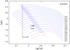 |
Fig. 6 Geneva evolution tracks for non-rotating stars without magnetic field for the metalicity Z = 0.014 (Mowlavi et al. 2012). The grey point is the luminosity value derived based on Gaia DR2 without the bolometriccorrection and dereddening. These corrections are applied for the black point. The colour of the evolutionary tracks distinguishes the A- and B-type stars. The vertical line shows the upper Teff limit determined by the best fit of the spectra. The column on the right-hand side of the graph denotes the stellar masses in M⊙. |
6 Discussion
6.1 IRAS 17449+2320’s place in FS CMa group
Even if the main spectral features of FS CMa stars are very similar, allowing for the creation of this group, members do differ from one another in various ways. This is natural because we are dealing with objects embedded within very extensive inhomogeneous circumstellar matter, where only a different angle of view changes the observed spectral and photometrical properties. Moreover, the presence of a secondary component is highly probable. The properties of the secondary as well as the orbital parameters affect the observed spectra. In the following, we point to the specific properties of IRAS 17449+2320. Since all the members of FS CMa group are not sufficiently studied, we can mostly compare only with the main representatives of FS CMa group FS CMa itself, MWC 342, HD 50138, MWC 623, and MWC 728.
The most remarkable differences are Hα V∕R changes (Sect. 4.2). The violet peak is frequently larger than the red one and once even 1.6 times. This has not been observed in FS CMa stars. The red peak is almost always stronger. Up to now, V∕R > 1 was detected for only one event in HD 50138 (Jeřábková et al. 2016, V∕R ~ 1.2) and V∕R ~ 1 in MWC 728 (Miroshnichenko et al. 2015).
The Hα line of IRAS 17449+2320 shows night-to-night variability. Such a rapid variability of the Hα line is atypical for FS CMa stars. We can find a rule in FS CMa stars – the absorption lines of the B-component are variable on the scale of days and emission on a scale of at least a week, ruling out IRAS 17449+2320. Other lines which show the night-to-night changes are these of O I, and two Fe II lines that are connected to UV transitions (Fig. A.6).
On the other hand, fully absorbed He I lines show no variability. Since He I lines are formed in the deeper regions of the stellar photosphere, we can conclude that IRAS 17449+2320 has a very stable photosphere. This is in contrast with the observations of other FS CMa stars, which show nigh-to-night changes, indicating very dynamic inner parts of the photosphere. Here, IRAS 17449+2320 also exhibits a stronger difference between the population of the triplet and singlet states. As triplet states have lower excitation energy than singlet states, they are highly populated in a low-density medium. This stronger overpopulation of He I lines points to the lower density of the circumstellar matter around IRAS 17449+2320.
6.2 Spectral type
Generally, it is very difficult to exactly determine the stellar parameters of objects with extended inhomogeneus atmospheres. Even if FS CMa stars are slow rotators (i.e., gravity darkening could be neglected in these cases), the application of synthetic spectra based on plane-parallel or spherically symmetric models has to be taken with caution because of their geometrically-thick and (in most cases) also optically-thick circumstellar disks.
Based on optical photometry and on the strength of the He I 4471 Å and Mg II 4481 Å lines, Miroshnichenko et al. (2007) estimated the spectral type A0 for IRAS 17449+2320. Condori et al. (2019) derived a temperature of 9200 ± 300 K (A1–A2) and luminosity class II or III from color indexes. They also used the equivalent width (EW) ratio of Mg II 4482 Å versus He I 4471 Å and He I 4713 Å versus Si II 6347 Å to determine Teff of 9500 ± 500 K (A0–A2) and 10 700 ± 1000 K, respectively. Unfortunately, they did not mention the method used for the EW calculation. Fitting the line profiles by the Voigt function, the error due to the Zeeman splitting would be included. Gaia measurements (DR2) give Teff  K (Table 5).
We show that the exact determination of the stellar parameters is even more difficult for IRAS 17449+2320. The best fit by a single star (Teff = 12 580 K, log g = 4.2, and vrot=11 km s−1, solar composition) is far from the observed spectrum (see Fig. A.10). It is highly probable that a hot source contributes to the spectrum. Even if we were not able to find the spectral lines of this source, strong UV radiation (Sect. 3.1), the autoionization lines (Sect. 2), and especially the spectral variability (Sect. 4.1) are indicators of the additional hot continuum source. We simulate it as a rapidly rotating secondary for the spectral fitting (Sect. 5.3). As the hot source has no strong spectral lines in the visible, only a lower limit of the Teff is possible to obtain. This affects the solution for the “primary” star, where it is only possible to determine an upper limit of Teff = 11 040 K. Our detailed line identification (Table B.3) rejects the lowest temperatures corresponding to the spectral types A1 and A2 because of the lack of many Fe I lines, which are missing at temperatures higher than 10 000 K (e.g. λλ 4107, 4110, 4113, 4114, 4126, 4128, 4135 Å, etc.). Taking into account all the measurements, a reasonable guess of the spectral type of IRAS 17449+2320 is A0 or B9.
6.3 Binarity
The only well-defined period (P = 36.1 ± 0.2 d) found by (Miroshnichenko et al., in prep.) is based on the intensity ratio of the Hα emission edges. They interpreted this period as being due to the orbit of a companion star. This may be correct since the Hα emission edges reflect the radial velocity changes, rather than the emission strength. However, generally, the interpretation of the period found based on the emission lines is not straightforward and the situation is even more complicated in IRAS 17449+2320. The complication arises from the magnetic field, which changes the region of the emission formation. Instead of being situated in the disk, the emission region might originate either from the open magnetic field lines in the polar regions of the star or from opaque structures, or clouds, that are trapped in the co-rotating magnetosphere. The presence of such clouds has been recently suggested through photometric observations of Landstreet’s star by Mikulášek et al. (2020). If this is the case, then the 36 d period is the stellar rotation period.
6.4 FS CMa stars as classical Be stars with the magnetic field
The discovery of the magnetic field in a FS CMa star opens up a consideration of whether these stars can be classical Be stars with a magnetic field either from the primary or from the secondary component. A detailed review of the magnetic field in classical Be stars is given by Rivinius et al. (2013). Summarizing the published studies, they show that even if there were discoveries of a magnetic field in classical Be stars, it was always close to the detection limit. Eventual follow-up studies did not confirm the detections. Bagnulo et al. (2012) consider that Be stars do not have magnetic fields larger than 100 G. Their data itself cannot exlude the possibility that there exists a Be star with larger magnetic field; however, their analysis shows that even if it exists, it would be very exceptional. A very detailed survey of the magnetic field in hot stars has been done by the Magnetism in Massive Stars (MiMeS) consortium. Preliminary results (Wade et al. 2012) show that even if the magnetic field was detected in about 6.5% of B-type stars, none of the 58 studied classical Be stars were among them. They discussed this finding and demonstrated that it is not an observation or data reduction problem.
The only Be star with a magnetic field is β Cep. However, Schnerr et al. (2006) showed that the magnetic field is connected with the primary B1 IV component and not with the classical Be secondary (B6–8). These discoveries reveal that the angular momentum losses during the evolution of a star (Landstreet et al. 2009) are sufficient to slow down the rotation speed so that the centrifugal force is not large enough to support the outflow from the star to create Be star in a late MS phase. Thus, β Cep points to the possibility that there can be a number of Be stars with magnetic secondaries. If the separation of the components is sufficiently small to perturb or destroy the Be star disk, the observed spectral properties would be similar to that what we observe in FS CMa stars. However, this is not the case for IRAS 17449+2320.
6.5 Post-MS evolution phase of magnetic Ap stars
Our discovery of the magnetic field may solve a long-standing problem (Mathys 2004) regarding the nature of post-MS evolution of magnetic Ap stars. Some of the lower-temperature FS CMa stars may be objects that we have been looking for a long time.
Landstreet et al. (2009) presented their results of a study of magnetic Ap stars in open clusters in order to follow the evolution of their magnetic fields. They found magnetic Ap stars through the entire MS phase, from ZAMS to TAMS. However, the strength of the magnetic field strongly decreases with age. This is a natural consequence of the ohmic decay, large-scale hydrodynamic flows, and stellar evolution – the expansion of the star and reduction of the convection core. The ohmic decay time of the fossil magnetic field itself is of the order of 1010−1011 years (Glagolevskij 2018), which is between one and two orders of magnitude longer that the MS lifetime (108−109 yr). As shown by Landstreet et al. (2009), there are still some magnetic stars at TAMS, especially among the more massive stars (3–4 M⊙), where the surface magnetic field reaches the values of ~500 G.
The first dredge-up should amplify the rest of the fossil magnetic field and cause the amount of matter transported into the circumstellar medium to be larger than in non-magnetic stars. The Ap origin of cool FS CMa stars is partially supported by other observations: (i) FS CMa stars are located at the end of the MS, or just after TAMS (Miroshnichenko 2017); (ii) Herpin et al. (2006) discovered magnetic fields in AGB stars: the measured values of B were in a range from 0 to 20 G; (iii) While classical Be stars rotate at or near the critical velocity, FS CMa do not show rapid rotation. The magnetic field reduces the stars’ angular momentum. The effect is so efficient that the rotation period can reach several decades (Landstreet et al. 2009).
Based on the HRD (Fig. 6), IRAS 17449+2320 should be a B-type star. However, our spectral fitting gives only the upper limit to the Teff because without the UV spectra, it is impossible to determine the temperature of the hot source. The Gaia magnitude also has to be affected by this hot source; therefore, the luminosity is probably slightly overestimated. Previously, Miroshnichenko et al. (2007) classified this star as A0 and Condori et al. (2019) determined the range of spectral types from A0 to A2 (see Sect. 6.2 for details). Taking these points into account, the post-main sequence phase of magnetic Ap stars should not be rejected.
6.6 Mergers
All three previous scenarios suffer from serious problems. The regular periodicity probably reflects the stellar rotation rather than the orbital motion. A classical Be star can not have a strong magnetic field. Rotation will slow down the star during the MS life-time and, thus, it will never become a classical Be star. Here, IRAS 17449+2320, the primary B-type star, is the one with the strong magnetic field. The observed properties point to the post-MS evolution stage of a magnetic Ap star. It will fulfill a gap in our observations and models, but the HRD (Fig. 6) is more favorable for the B-type star near the end of its MS life. To explain the observed properties – the strong magnetic field, strong IR excess, relatively stable envelope, and the position on the HRD – merger theory provides a good fit.
Schneider et al. (2020) show that the strong mag. field can be generated during the merger. A strong magnetic field can survive the MS evolution because the ohmic decay time is longer than the MS lifetime. The stronger the magnetic field, the faster the merged star slows its rotation. The enrichment of the heavy elements in the photosphere may be detected. However, how large this effect is depends on the age of original stars and other factors. For young stars anomalous surface composition does not have to be detected. The merger hypothesis naturally explains the large amount of the circumstellar material. Material is ejected: (i) before the merger through the L2 point; (ii) during the merger process; (iii) after the merger, the resulting star rotates with the critical velocity allowing the creation of the decretion disk; or (iv) in some cases, the Eddington limit may be crossed leading to additional mass loss, while some of the ejected material may be re-accreting to the final star.
The merger hypothesis is very promising. The question remains as to whether the merging of binaries has sufficiently high probability. Soker & Tylenda (2006) have presented their assumption that there may be one V838 Mon-like outburst every 10–50 yr in the galaxy. However, the creation of a very bright event is not the only channel for the merging process (Soker & Tylenda 2006). Moreover, they did not take into account the formation of binaries (e.g., Bate et al. 2002) and evolution of young clusters (Bate 2019). Indeed, the simulations of recently formed realistic binary-star-rich clusters lead to the formation of “forbidden binaries” that are characterized by large orbital eccentricities and short periods, leading the companion stars to merge (Kroupa 1995). Recent works on this problem have shown a high ejection rate of massive stars from their birth clusters and also reveal that a large fraction of B and O-type stars undergo mergers because of the stellar-dynamical encounters in the compact young clusters (Oh et al. 2015; Oh & Kroupa 2016, 2018). The profusion of mergers, particularly among massive stars, are likely tobe part of the explanation of the elemental peculiarities observed in globular cluster stars (Wang et al. 2020). In any population, mergers of stars formed in binaries with B-type and also M-dwarf companion masses are thus likely to be common. This aspect will be addressed in the future through simulations. Examples of observed remnants of recent mergers have been monitored (Kamiński et al. 2015; Tylenda & Kamiński 2016). Moreover, according to current simulations, the binaries ejected from young clusters merge soon after leaving the cluster (F. Dinnbier, priv. comm.). This is the natural consequence of the angular momentum change.
This possible phase of the past evolution has to reveal itself in the proper motion. Indeed, Gaia measurements of IRAS 17449+2320 (Table 5) give the space velocities U = −26.119, V = −4.595, and W = 7.614 km s−1 (Czesla et al. 2019). In comparing these values with the results of an extended study of Nordström et al. (2004), we can see that IRAS 17449+2320 has slightly higher velocities than most of the stars in the solar neighborhood. However, due to the heating of the galactic disk by spiral arms, or giant molecular clouds, we also have to take into account the age of stars for the comparison of the space velocities of their stellar sample and IRAS 17449+2320. According to the HRD (Fig. 6, bottom panel), IRAS 17449+2320 is about 0.5 Gy old. Among these young stars, IRAS 17449+2320 is an outlier. The W velocity, which is the component of the space speed toward the north Galactic pole, is a particularly large outlier. Based on a more detailed analysis of Gaia DR2 data, Boubert & Evans (2018) also concluded that IRAS 17449+2320 is very likely to be a runaway star. This brings the strong support for the scenario of the merger binary ejected from a young cluster.
7 Conclusions
We found the presence of a magnetic field in IRAS 17449+2320, which is the first detection in FS CMa type stars. The magnetic field is very strong, leading to a clear Zeeman-splitting of many lines, on the basis of which we derived a mean magnetic field modulus of 6.2 ± 0.2 kG. The magnetic field detection changes our view of the nature of FS CMa stars. This opens up the possibility that these objects are classical Be stars, the secondary component of which would have a strong magnetic field and be sufficiently close to the primary to disturb or destroy the disk. The magnetic field can hardly be connected with a classical Be star because it slows down the rotation speed during the MS evolution. Therefore, the centrifugal force is too low to support the creation of the decretion disk at the end of the MS. Indeed, no Be stars with a magnetic field have been detected thus far (Wade et al. 2012). Contrary to this assumption, radial velocities and magnetic splitting of the lines show that the magnetic field is connected with the primary A/B-type star of IRAS 17449+2320.
Our observations show that IRAS 17449+2320 is a slightly atypical FS CMa star. Moreover, it is among the cooler FS CMa stars. Previously, the spectral type from A0 to A2 had been determined (Miroshnichenko et al. 2007; Condori et al. 2019, see Sect. 6.2). These are hints that we may be dealing with a different type of object. Because the spectrum of IRAS 17449+2320 is very similar to magnetic Ap stars (e.g., Figs. 5 and A.8), it allows for the possibility that this star could be a magnetic Ap star at an evolutionary stage just after TAMS. No such star has been discovered thus far, although some magnetic Ap stars with strong magnetic fields have also been found to be located at TAMS (Landstreet et al. 2009). Contrary to this hypothesis, we have the position of IRAS 17449+2320 on the HRD (Fig. 6), leading us to surmise that we are dealing with B-type star. However, the observed variability of spectral lines (intensity of which is reducing and amplifying simultaneously) and the spectral fitting reveal the presence of a hot source (> 50 000 K). It may be either a secondary component, or a source connected with the magnetic field. Because there are no spectral lines of the hot component in the visible part of the spectra, the spectral fitting gives only the upper temperature limit of the primary (~11 000 K). The hot source must also be affecting the Gaia measurements, leading to an overestimate of the luminosity.
A strong magnetic field, strong IR excess, emission lines, as well as forbidden emission lines, a relatively stable envelope, and its position on the HRD may be explained as the features of a merger system. A magnetic field, even a very strong one, may have been generated during the merger (Schneider et al. 2020). Due to the magnetic field, the merger product slows down very quickly, as it is observed in FS CMa stars. The material is ejected before, during, and after the merger, leading to the creation of a massive disk. Current calculations show that the escaped binaries from the clusters have to merge soon after leaving the cluster. IRAS 17449+2320 may be one of these cases, because its component of the space velocity toward the north Galactic pole is significantly larger (W = 8.47 km s−1) than is observed in stars in the solar neighbourhood Nordström et al. (2004). Boubert & Evans (2018) also classified IRAS 17449+2320 as a runaway star based on Gaia DR2 data.
The presence of a hot source points to the binary nature of IRAS 17449+2320, where the secondary is a hot dwarf because it contributes less than 40% to the total bolometric flux of the system (Sect. 5.3). The current binary nature of the system is supported by the periodic variations of the Hα emission wing edges and EWs (36.1 d, Miroshnichenko et al., in prep.). On the other hand, the variability of the emission parts of lines, especially the Hα line, does not actually prove orbital motion in a binary system. Especially in this case, the emission may originate in the plasma trapped by the strong magnetic field above the surface (Mikulášek et al. 2020).
IRAS 17449+2320 does not show all of the typical features of the main representatives of FS CMa stars (Korčáková et al., in prep.). The absorption lines of He and metals, with the exception of the O I lines, are remarkably stable. The night-to-night variability is observed only in H, O I, and two Fe II lines that are directly connected with the UV transitions. This behavior is contrary to what is seen in other FS CMa stars. The detection of Hα V∕R > 1 in IRAS 17449+2320 is also very rare.
Another phenomenon that has been observed for the first time in FS CMa stars is the opposite behavior with regard to Balmer and O I lines as compared to other lines. We observed at certain epochs the appearance of the strong red wing absorption in Balmer lines and the O I triplet λλ 7772, 7774, and 7775 Å, as well as O I line 8446 Å (Fig. 2). No other line profile is affected, which is very unusual. The other lines show only an intensity decrease or increase, depending on the position in the spectra. This indicates changes in the continuum radiation. Longward from ~6300 Å, the continuum intensity is slightly lower, whereas shortward it is slightly higher. It is possible that in these phases, what we are seeing is thesecondary component. Alternatively, the stellar surface of the magnetic star, which is not blocked by the circumstellar matter distributed along the magnetic field lines close to the poles, is visible in these phases. The rotation is fully responsible for the spectral variability in this case. We noticed a larger contrast in the population of singlet and triplet states of He I lines, which points to a lower density material than that of other FS CMa stars. This is supported also by the great number of H levels. We were able to identify the lines from the 28th level.
IRAS 17449+2320 has strong UV radiation (Table 2). Even without knowledge of its UV spectra, we can deduce its basic character from the visible lines. Since we do not observe emission wings of metal lines, which are affected by cascade transitions in FS CMa stars, there may not be an iron curtain at work here. On the other hand, the absence of the iron curtain might only be a geometrical effect. If we do not see the disk almost edge-on, absorption of the iron group elements would not be so strong, nor would it be the case for the Li I lines. We detected two episodes of material infall, revealed by the narrow discrete absorption components in the resonance lines. Usually, material outflow is detected in FS CMa stars, but the inflow events are not exceptional (Korčáková et al., in prep.).
From the first spectrum of IRAS 17449+2320, it became obvious that we are dealing with an object that can help reveal the nature of FS CMa stars. After obtaining high-resolution spectra, we found a Zeeman-splitting of the magnetically active lines. This was a proof that the magnetic field has to be taken into account in the discussion of the nature of FS CMa stars. The strong magnetic field, observed spectral properties, and variability, taken together with the high space velocity toward the galactic pole, point to a merger as the most likely scenario for IRAS 17449+2320.
Acknowledgements
We appreciate the work of the referees, whose valuable comments helped to improve the paper. We would like to thank A. Miroshnichenko, S. V. Zharikov, and F. Dinnbier for the valuable comments and P. Zasche, M. Wolf, P. Berardi, and P. Škoda for some spectra. The research of D.K. is supported by grant GA 17-00871S of the Czech Science Foundation. P.K. acknowledges support from the Grant Agency of the Czech Republic under grant number 20-21855S and the DAAD Bonn-Prague exchange programme. A.R. acknowledges the Research Associate Fellowship with order no. 03(1428)/18/EMR-II under Council of Scientific and Industrial Research (CSIR). This work has made use of data from the European Space Agency (ESA) mission Gaia (https://www.cosmos.esa.int/gaia), processed by the Gaia Data Processing and Analysis Consortium (DPAC, https://www.cosmos.esa.int/web/gaia/dpac/consortium). Funding for the DPAC has been provided by national institutions, in particular the institutions participating in the Gaia Multilateral Agreement. Based on data from Perek 2 m telescope, Ondřejov, Czech Republic. Based on observations obtained at the Canada-France-Hawaii Telescope (CFHT) which is operated by the National Research Council of Canada, the Institut National des Sciences de l’Univers of the Centre National de la Recherche Scientique of France, and the University of Hawaii. The observations at the Canada-France-Hawaii Telescope were performed with care and respect from the summit of Maunakea which is a significant cultural and historic site. This work uses NIST database Kramida et al. (2018). NIST Atomic Spectra Database (ver. 5.6.1), [Online]. Available: https://physics.nist.gov/asd [2019, May 25]. National Institute of Standards and Technology, Gaithersburg, MD. DOI: https://doi.org/10.18434/T4W30F, and van Hoof (2018) line list and database.
Appendix A Additional figures
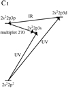 |
Fig. A.1 Formation of the strongest C I lines in the visible from the multiplet 270; λλ 9 061, 9 062, 9 078, 9 089, 9 095, 9 112 Å. The level 2s2 2p3s is strongly populated by the UV resonance transition, which al- lows the absorption lines to the level 2s22p3p. However, the upper level from this transition is also populated from the level 2s2 2p3d pumped by UV radiation. This overpopulation of 2s22p3p creates the emission wings of these strongest lines. |
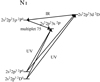 |
Fig. A.2 Formation of the emission wings of lines 8 594.00 and 8 629.24 Å of N I from the multiplet 75. The UV radiation pumps the level 2s22p23d 2D as well as the level 2s22p23s 2P, thanks to which the absorption core is observed. The level 2s22p23d 2D is connected straightforward with the ground level by the very strong resonance line. However, the energy difference of the levels (corresponding to the ~ 950 Å) is to high for the UV radiation outgoing from the star. The sharp fall around 900 Å is the common property of FS CMa objects (Korčáková et al., in press). Indeed, we found no line corresponding to this level in the spectrum. |
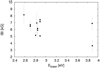 |
Fig. A.3 Mean magnetic field modulus of Fe II lines in dependence of the energy of the lower level. |
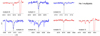 |
Fig. A.4 Position, strength, and shape of He I lines. The vertical lines denote the central wavelength of the lines and the horizontal line the position of the continuum. The color distinguishes the singlet (red) and triplets (blue) states. All spectral lines are plotted on the same scale, which suppresses the strength of the emission wings of He I 5 876 and 6 678 Å lines. We note that the continuum normalization was carried out very carefully. |
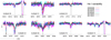 |
Fig. A.5 Variability of He I lines. The plotted spectra come from CFHT, which provides the highest available resolution. |
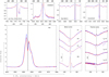 |
Fig. A.6 Night-to-night changes demonstrated on the spectra taken at CFHT on 2012-08-13 and 2012-08-14. Significant changes are shown only in the hydrogen and oxygen lines. Also shown to be slightly different is the blue wing of the Fe II lines 4 924, and 5 018 Å lines. Other lines do not show night-to-night variations. The spectra are corrected on the system radial velocity. The laboratory wavelength connected with the system is plotted by the vertical grey line and its thickness corresponds to its error. |
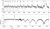 |
Fig. A.7 Paschen series. The labels denote the upper level of the transition. |
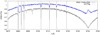 |
Fig. A.8 Comparison of N I multiplet 60 of IRAS 17449+2320 with a metallic Am star o Peg (A1 IV). The magnetic field of o Peg reaches the value of 2 kG (Mathys & Lanz 1990). The figure also shows the Paschen line 8 750.46 Å. |
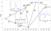 |
Fig. A.9 Grotrian of the neutral oxygen. |
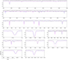 |
Fig. A.10 Spectral fitting. The observed spectrum is plotted by the black line, the blue one is the best fit using PYTERPOL code (see Table 4), for which the contribution of the hot source was included into the calculations. For the comparison, we also show the best fit by a single star (Teff = 12 580 K, log g =4.2, and vrot =11 km s−1, solar composition) without the contribution of a hot source, the dotted violet line. |
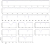 |
Fig. A.11 Spectral fitting. The observed spectrum is plotted by the black line, the blue one is the best fit using PYTERPOL code, a starwith the contribution of the hot source. The grey line is the individual spectrum of the primary, that is, without the contribution of the hot source. |
Appendix B Additional tables
Mean magnetic field modulus |B|.
List of observations.
Line list.
Notes.
| E | emission line | Z | Zeeman split | iA | interstellar absorption |
| A | absoprtion line | 2Z | double peak | DIB | diffuse interstellar bands |
| EC | emission core | 3Z | triple peak | ⋆ | Ritz wavelength (NIST database) |
| a | autoionisation line | 4Z | four peaks | ⋆⋆ | Van Hoof’s line list (van Hoof 2018) |
References
- Adelman, S. J. 1974, ApJS, 28, 51 [NASA ADS] [CrossRef] [Google Scholar]
- Allen, D. A., & Swings, J. P. 1976, A&A, 47, 293 [NASA ADS] [Google Scholar]
- Aret, A., Kraus, M., & Šlechta M. 2016, MNRAS, 456, 1424 [NASA ADS] [CrossRef] [Google Scholar]
- Aslanov, I. A., & Rustamov, Y. S. 1976, IAU Colloq., 32, 613 [NASA ADS] [Google Scholar]
- Bagnulo, S., Landstreet, J. D., Fossati, L., & Kochukhov, O. 2012, A&A, 538, A129 [NASA ADS] [CrossRef] [EDP Sciences] [Google Scholar]
- Bate, M. R. 2019, MNRAS, 484, 2341 [NASA ADS] [CrossRef] [Google Scholar]
- Bate, M. R., Bonnell, I. A., & Bromm, V. 2002, MNRAS, 336, 705 [Google Scholar]
- Boubert, D., & Evans, N. W. 2018, MNRAS, 477, 5261 [Google Scholar]
- Carciofi, A. C., Miroshnichenko, A. S., & Bjorkman, J. E. 2010, ApJ, 721, 1079 [NASA ADS] [CrossRef] [Google Scholar]
- Cardelli, J. A., Clayton, G. C., & Mathis, J. S. 1989, ApJ, 345, 245 [Google Scholar]
- Chkhikvadze, J. N., Kakhiani, V. O., & Djaniashvili, E. B. 2002, Astrophysics, 45, 8 [NASA ADS] [CrossRef] [Google Scholar]
- Condori, C. A. H., Borges Fernandes, M., Kraus, M., Panoglou, D., & Guerrero, C. A. 2019, MNRAS, 488, 1090 [NASA ADS] [CrossRef] [Google Scholar]
- Czesla, S., Schröter, S., Schneider, C. P., et al. 2019, PyA: Python astronomy-related packages [Google Scholar]
- de Freitas Pacheco, J. A., Gilra, D. P., & Pottasch, S. R. 1982, A&A, 108, 111 [NASA ADS] [Google Scholar]
- de la Fuente, D., Najarro, F., Trombley, C., Davies, B., & Figer, D. F. 2015, A&A, 575, A10 [NASA ADS] [CrossRef] [EDP Sciences] [Google Scholar]
- de Laverny, P., Recio-Blanco, A., Worley, C. C., & Plez, B. 2012, A&A, 544, A126 [NASA ADS] [CrossRef] [EDP Sciences] [Google Scholar]
- Fischer, C. F., Tachiev, G., Gaigalas, G., & Godefroid, M. R. 2007, Comput. Phys. Commun., 176, 559 [NASA ADS] [CrossRef] [Google Scholar]
- Gaia Collaboration (Prusti, T., et al.) 2016, A&A, 595, A1 [NASA ADS] [CrossRef] [EDP Sciences] [Google Scholar]
- Gaia Collaboration (Brown, A. G. A., et al.) 2021, A&A, 649, A1 [NASA ADS] [CrossRef] [EDP Sciences] [Google Scholar]
- Galazutdinov, G. A., Musaev, F. A., Krełowski, J., & Walker, G. A. H. 2000, PASP, 112, 648 [NASA ADS] [CrossRef] [Google Scholar]
- Glagolevskij, Y. V. 2018, Astrophysics, 61, 546 [NASA ADS] [CrossRef] [Google Scholar]
- Herpin, F., Baudry, A., Thum, C., Morris, D., & Wiesemeyer, H. 2006, A&A, 450, 667 [NASA ADS] [CrossRef] [EDP Sciences] [Google Scholar]
- Horvat, M., Conroy, K. E., Pablo, H., et al. 2018, ApJS, 237, 26 [Google Scholar]
- Inglis, D. R., & Teller, E. 1939, ApJ, 90, 439 [NASA ADS] [CrossRef] [Google Scholar]
- Jeřábková, T., Korčáková, D., Miroshnichenko, A., et al. 2016, A&A, 586, A116 [NASA ADS] [CrossRef] [EDP Sciences] [Google Scholar]
- Kamiński, T., Mason, E., Tylenda, R., & Schmidt, M. R. 2015, A&A, 580, A34 [NASA ADS] [CrossRef] [EDP Sciences] [Google Scholar]
- Khokhlov, S. A., Miroshnichenko, A. S., Mennickent, R., et al. 2017, ApJ, 835, 53 [NASA ADS] [CrossRef] [Google Scholar]
- Khokhlov, S. A., Miroshnichenko, A. S., Zharikov, S. V., et al. 2018, ApJ, 856, 158 [NASA ADS] [CrossRef] [Google Scholar]
- Kluska, J., Benisty, M., Soulez, F., et al. 2016, A&A, 591, A82 [NASA ADS] [CrossRef] [EDP Sciences] [Google Scholar]
- Korčáková, D., Shore, S. N., Miroshnichenko, A., et al. 2019, ASP Conf. Ser., 519, 155 [Google Scholar]
- Korčáková, D., Miroshnichenko, A. S., Zharikov, S. V., et al. 2020, Mem. Soc. Astron. It., 91, 118 [Google Scholar]
- Kramida, A., Ralchenko, Yu., Reader, J., & NIST ASD Team 2018, NIST Atomic Spectra Database (ver. 5.6.1), [Online]. Available: https://physics.nist.gov/asd [2019, May 14]. National Institute of Standards and Technology, Gaithersburg, MD [Google Scholar]
- Kroupa, P. 1995, MNRAS, 277, 1507 [NASA ADS] [Google Scholar]
- Kurucz, R. L. 2005, Mem. Soc. Astron. It. Suppl., 8, 14 [Google Scholar]
- Kučerová, B., Korčáková, D., Polster, J., et al. 2013, A&A, 554, A143 [NASA ADS] [CrossRef] [EDP Sciences] [Google Scholar]
- Lamers, H. J. G. L. M., Zickgraf, F.-J., de Winter, D., Houziaux, L., & Zorec, J. 1998, A&A, 340, 117 [NASA ADS] [Google Scholar]
- Landstreet, J. D., Bagnulo, S., Andretta, V., et al. 2009, ASP Conf. Ser., 405, 505 [NASA ADS] [Google Scholar]
- Lanz, T., & Hubeny, I. 2003, ApJS, 146, 417 [NASA ADS] [CrossRef] [Google Scholar]
- Lanz, T., & Hubeny, I. 2007, ApJS, 169, 83 [CrossRef] [Google Scholar]
- Lozitsky, V. G., & Staude, J. 2009, JA&A, 29, 387 [NASA ADS] [Google Scholar]
- Maeder, A., & Meynet, G. 2004, A&A, 422, 225 [NASA ADS] [CrossRef] [EDP Sciences] [Google Scholar]
- Mathys, G. 2004, IAU Symp., 224, 225 [NASA ADS] [CrossRef] [Google Scholar]
- Mathys, G. 2017, A&A, 601, A14 [NASA ADS] [CrossRef] [EDP Sciences] [Google Scholar]
- Mathys, G., & Lanz, T. 1990, A&A, 230, L21 [NASA ADS] [Google Scholar]
- Mel’Nikov, S. Y. 1997, Astron. Lett., 23, 799 [Google Scholar]
- Mikulášek, Z., Zverko, J., Romanyuk, I. I., et al. 2004, Magnetic Stars (USA: NASA), 191 [Google Scholar]
- Mikulášek, Z., Krtička, J., Shultz, M. E., et al. 2020, in Stellar Magnetism: A Workshop in Honour of the Career and Contributions of John D. Landstreet, eds. G. Wade, E. Alecian, D. Bohlender, & A. Sigut, 11, 46 [Google Scholar]
- Miroshnichenko, A. S. 2007, ApJ, 667, 497 [NASA ADS] [CrossRef] [Google Scholar]
- Miroshnichenko, A. S. 2017, ASP Conf. Ser., 508, 285 [NASA ADS] [Google Scholar]
- Miroshnichenko, A. S., & Zharikov, S. V. 2015, EAS Pub. Ser., 71–72, 181 [Google Scholar]
- Miroshnichenko, A. S., Chentsov, E. L., Klochkova, V. G., et al. 2000, A&AS, 147, 5 [NASA ADS] [CrossRef] [EDP Sciences] [Google Scholar]
- Miroshnichenko, A. S., Manset, N., Kusakin, A. V., et al. 2007, ApJ, 671, 828 [NASA ADS] [CrossRef] [Google Scholar]
- Miroshnichenko, A. S., Manset, N., Polcaro, F., Rossi, C., & Zharikov, S. 2011, IAU Symp. 272, 260 [NASA ADS] [Google Scholar]
- Miroshnichenko, A. S., Zharikov, S. V., Danford, S., et al. 2015, ApJ, 809, 129 [NASA ADS] [CrossRef] [Google Scholar]
- Miroshnichenko, A. S., Polcaro, V. F., Rossi, C., et al. 2017, ASP Conf. Ser., 508, 387 [NASA ADS] [Google Scholar]
- Miroshnichenko, A. S., Danford, S., Zharikov, S. V., et al. 2020a, ApJ, 897, 48 [NASA ADS] [CrossRef] [Google Scholar]
- Miroshnichenko, A. S., Zharikov, S. V., Korčaková, D., et al. 2020b, Contrib. Astron. Observ. Skal. Pleso, 50, 513 [NASA ADS] [Google Scholar]
- Mowlavi, N., Eggenberger, P., Meynet, G., et al. 2012, A&A, 541, A41 [NASA ADS] [CrossRef] [EDP Sciences] [Google Scholar]
- Nemravová, J. A., Harmanec, P., Brož, M., et al. 2016, A&A, 594, A55 [Google Scholar]
- Nesvacil, N., Hubrig, S., & Jehin, E. 2004, A&A, 422, L51 [NASA ADS] [CrossRef] [EDP Sciences] [Google Scholar]
- Nissen, W. 1954, Z. Phys., 139, 638 [NASA ADS] [CrossRef] [Google Scholar]
- Nordström, B., Mayor, M., Andersen, J., et al. 2004, A&A, 418, 989 [Google Scholar]
- O’Donnell, J. E. 1994, ApJ, 422, 158 [Google Scholar]
- Oh, S., & Kroupa, P. 2016, A&A, 590, A107 [NASA ADS] [CrossRef] [EDP Sciences] [Google Scholar]
- Oh, S., & Kroupa, P. 2018, MNRAS, 481, 153 [NASA ADS] [CrossRef] [Google Scholar]
- Oh, S., Kroupa, P., & Pflamm-Altenburg, J. 2015, ApJ, 805, 92 [Google Scholar]
- Palacios, A., Gebran, M., Josselin, E., et al. 2010, A&A, 516, A13 [NASA ADS] [CrossRef] [EDP Sciences] [Google Scholar]
- Pedersen, M. G., Escorza, A., Pápics, P. I., & Aerts, C. 2020, MNRAS, 495, 2738 [Google Scholar]
- Plavchan, P., Jura, M., Kirkpatrick, J. D., Cutri, R. M., & Gallagher, S. C. 2008, ApJS, 175, 191 [NASA ADS] [CrossRef] [Google Scholar]
- Pogodin, M. A. 1997, A&A, 317, 185 [NASA ADS] [Google Scholar]
- Polster, J., Korčáková, D., Votruba, V., et al. 2012, A&A, 542, A57 [NASA ADS] [CrossRef] [EDP Sciences] [Google Scholar]
- Polster, J., Korčáková, D., & Manset, N. 2018, A&A, 617, A79 [NASA ADS] [CrossRef] [EDP Sciences] [Google Scholar]
- Press, W. H., & Teukolsky, S. A. 1988, Comput. Phys., 2, 77 [NASA ADS] [CrossRef] [Google Scholar]
- Prša, A., & Zwitter, T. 2005, ApJ, 628, 426 [Google Scholar]
- Prša, A., Conroy, K. E., Horvat, M., et al. 2016, ApJS, 227, 29 [Google Scholar]
- Pych, W. 2004, PASP, 116, 148 [NASA ADS] [CrossRef] [Google Scholar]
- Rivinius, T., Carciofi, A. C., & Martayan, C. 2013, A&ARv, 21, 69 [Google Scholar]
- Schlegel, D. J., Finkbeiner, D. P., & Davis, M. 1998, ApJ, 500, 525 [Google Scholar]
- Schneider, F. R. N., Ohlmann, S. T., Podsiadlowski, P., et al. 2020, MNRAS, 495, 2796 [NASA ADS] [CrossRef] [Google Scholar]
- Schnerr, R. S., Henrichs, H. F., Oudmaijer, R. D., & Telting, J. H. 2006, A&A, 459, L21 [NASA ADS] [CrossRef] [EDP Sciences] [Google Scholar]
- Shevchenko, V. S., Grankin, K. N., Ibragimov, M. A., Mel’Nikov, S. Y., & Yakubov, S. D. 1993, Ap&SS, 202, 121 [NASA ADS] [CrossRef] [Google Scholar]
- Silvester, J., Kochukhov, O., & Wade, G. A. 2014, MNRAS, 444, 1442 [NASA ADS] [CrossRef] [Google Scholar]
- Soker, N., & Tylenda, R. 2006, MNRAS, 373, 733 [NASA ADS] [CrossRef] [Google Scholar]
- Tylenda, R., & Kamiński, T. 2016, A&A, 592, A134 [NASA ADS] [CrossRef] [EDP Sciences] [Google Scholar]
- van Hoof, P. A. M. 2018, Galaxies, 6, 63 [NASA ADS] [CrossRef] [Google Scholar]
- Wade, G. A., Grunhut, J. H., & MiMeS Collaboration 2012, ASP Conf. Ser., 464, 405 [NASA ADS] [Google Scholar]
- Wang, L., Kroupa, P., Takahashi, K., & Jerabkova, T. 2020, MNRAS, 491, 440 [Google Scholar]
- Wolber, G., Figger, H., Haberstroh, R. A., & Penselin, S. 1970, Z. Phys., 236, 337 [NASA ADS] [CrossRef] [Google Scholar]
- Wszolek, B. 2006, in 13th Young Scientists’ Conference on Astronomy and Space Physics, eds. A. Golovin, G. Ivashchenko, & A. Simon, 5 [Google Scholar]
- Zickgraf, F. J., & Schulte-Ladbeck, R. E. 1989, A&A, 214, 274 [NASA ADS] [Google Scholar]
Spectra are available at the CDS database.
IRAF is distributed by the National Optical Astronomy Observatories, operated by the Association of Universities for Research in Astronomy, Inc., under contract to the National Science Foundation of the United States.
All Tables
All Figures
|
Fig. 1 Discrete components of the resonance lines. The events were captured on the SPM spectra on 2013-10-16, following the spectrum over five days, and on 2018-09-25. |
| In the text | |
|
Fig. 2 Comparison of the selected parts of the spectra for phases showing the red-shifted absorption (CFHT 2012-02-09, blue lines) and a regular spectrum (CFHT 2006-06-08, red lines). The spectra are corrected on system velocity determined based on the position of [O I] lines. The area with C I multiplet is contaminated by the atmospheric lines. |
| In the text | |
|
Fig. 3 Selected Hβ line profiles from CFHT. Upper panel: remarkably stable wings lasting more than decade, while bottom panel: variable core. The grey arrow on the upper panel and grey vertical line on the bottom panel denote the system velocity position. |
| In the text | |
|
Fig. 4 V∕R changes of the Hα line and its periodogram. The horizontal line in the upper panel shows the V∕R = 1 level. Most FS CMa stars have V∕R ratios belowthis line. |
| In the text | |
|
Fig. 5 Comparison of selected Fe I and Mg I lines of IRAS 17447+2320 and the Ap star HD 51684 (F0p) with the value of the mean magnetic field modulus: 6 027 ± 50 G (Mathys 2017). |
| In the text | |
|
Fig. 6 Geneva evolution tracks for non-rotating stars without magnetic field for the metalicity Z = 0.014 (Mowlavi et al. 2012). The grey point is the luminosity value derived based on Gaia DR2 without the bolometriccorrection and dereddening. These corrections are applied for the black point. The colour of the evolutionary tracks distinguishes the A- and B-type stars. The vertical line shows the upper Teff limit determined by the best fit of the spectra. The column on the right-hand side of the graph denotes the stellar masses in M⊙. |
| In the text | |
|
Fig. A.1 Formation of the strongest C I lines in the visible from the multiplet 270; λλ 9 061, 9 062, 9 078, 9 089, 9 095, 9 112 Å. The level 2s2 2p3s is strongly populated by the UV resonance transition, which al- lows the absorption lines to the level 2s22p3p. However, the upper level from this transition is also populated from the level 2s2 2p3d pumped by UV radiation. This overpopulation of 2s22p3p creates the emission wings of these strongest lines. |
| In the text | |
|
Fig. A.2 Formation of the emission wings of lines 8 594.00 and 8 629.24 Å of N I from the multiplet 75. The UV radiation pumps the level 2s22p23d 2D as well as the level 2s22p23s 2P, thanks to which the absorption core is observed. The level 2s22p23d 2D is connected straightforward with the ground level by the very strong resonance line. However, the energy difference of the levels (corresponding to the ~ 950 Å) is to high for the UV radiation outgoing from the star. The sharp fall around 900 Å is the common property of FS CMa objects (Korčáková et al., in press). Indeed, we found no line corresponding to this level in the spectrum. |
| In the text | |
|
Fig. A.3 Mean magnetic field modulus of Fe II lines in dependence of the energy of the lower level. |
| In the text | |
|
Fig. A.4 Position, strength, and shape of He I lines. The vertical lines denote the central wavelength of the lines and the horizontal line the position of the continuum. The color distinguishes the singlet (red) and triplets (blue) states. All spectral lines are plotted on the same scale, which suppresses the strength of the emission wings of He I 5 876 and 6 678 Å lines. We note that the continuum normalization was carried out very carefully. |
| In the text | |
|
Fig. A.5 Variability of He I lines. The plotted spectra come from CFHT, which provides the highest available resolution. |
| In the text | |
|
Fig. A.6 Night-to-night changes demonstrated on the spectra taken at CFHT on 2012-08-13 and 2012-08-14. Significant changes are shown only in the hydrogen and oxygen lines. Also shown to be slightly different is the blue wing of the Fe II lines 4 924, and 5 018 Å lines. Other lines do not show night-to-night variations. The spectra are corrected on the system radial velocity. The laboratory wavelength connected with the system is plotted by the vertical grey line and its thickness corresponds to its error. |
| In the text | |
|
Fig. A.7 Paschen series. The labels denote the upper level of the transition. |
| In the text | |
|
Fig. A.8 Comparison of N I multiplet 60 of IRAS 17449+2320 with a metallic Am star o Peg (A1 IV). The magnetic field of o Peg reaches the value of 2 kG (Mathys & Lanz 1990). The figure also shows the Paschen line 8 750.46 Å. |
| In the text | |
|
Fig. A.9 Grotrian of the neutral oxygen. |
| In the text | |
|
Fig. A.10 Spectral fitting. The observed spectrum is plotted by the black line, the blue one is the best fit using PYTERPOL code (see Table 4), for which the contribution of the hot source was included into the calculations. For the comparison, we also show the best fit by a single star (Teff = 12 580 K, log g =4.2, and vrot =11 km s−1, solar composition) without the contribution of a hot source, the dotted violet line. |
| In the text | |
|
Fig. A.11 Spectral fitting. The observed spectrum is plotted by the black line, the blue one is the best fit using PYTERPOL code, a starwith the contribution of the hot source. The grey line is the individual spectrum of the primary, that is, without the contribution of the hot source. |
| In the text | |
Current usage metrics show cumulative count of Article Views (full-text article views including HTML views, PDF and ePub downloads, according to the available data) and Abstracts Views on Vision4Press platform.
Data correspond to usage on the plateform after 2015. The current usage metrics is available 48-96 hours after online publication and is updated daily on week days.
Initial download of the metrics may take a while.