| Issue |
A&A
Volume 658, February 2022
|
|
|---|---|---|
| Article Number | A11 | |
| Number of page(s) | 32 | |
| Section | Extragalactic astronomy | |
| DOI | https://doi.org/10.1051/0004-6361/202140403 | |
| Published online | 27 January 2022 | |
Radio data challenge the broadband modelling of GRB 160131A afterglow
1
INAF – Osservatorio Astronomico di Cagliari, Via della Scienza 5, 09047 Selargius, Italy
e-mail: marco.marongiu@inaf.it
2
Department of Physics and Earth Science, University of Ferrara, Via Saragat 1, 44122 Ferrara, Italy
3
ICRANet, Piazzale della Repubblica 10, 65122 Pescara, Italy
4
INFN – Sezione di Ferrara, Via Saragat 1, 44122 Ferrara, Italy
5
INAF – Osservatorio di Astrofisica e Scienza dello Spazio di Bologna, Via Piero Gobetti 101, 40129 Bologna, Italy
6
INAF – Istituto di Astrofisica e Planetologia Spaziali, Via Fosso del Cavaliere 100, 00133 Rome, Italy
7
Center for Astrophysics and Cosmology, University of Nova Gorica, Vipavska 13, 5000 Nova Gorica, Slovenia
8
Department of Physics, University of Bath, Claverton Down, Bath BA2 7AY, UK
9
Department of Astronomy, University of Maryland, College Park, MD 20742–4111, USA
10
Astrophysics Science Division, NASA Goddard Space Flight Center, 8800 Greenbelt Rd, Greenbelt, MD 20771, USA
11
Department of Astronomy and Astrophysics, The Pennsylvania State University, 525 Davey Lab, University Park, PA 16802, USA
12
Astrophysics Research Institute, Liverpool John Moores University, IC2, Liverpool Science Park, 146 Brownlow Hill, Liverpool L3 5RF, UK
13
Faculty of Mathematics and Physics, University of Ljubljana, Jadranska 19, Ljubljana 1000, Slovenia
Received:
22
January
2021
Accepted:
28
October
2021
Context. Gamma-ray burst (GRB) afterglows originate from the interaction between the relativistic ejecta and the surrounding medium. Consequently, their properties depend on several aspects: radiation mechanisms, relativistic shock micro-physics, circumburst environment, and the structure and geometry of the relativistic jet. While the standard afterglow model accounts for the overall spectral and temporal evolution for a number of GRBs, its validity limits emerge when the data set is particularly rich and constraining, especially in the radio band.
Aims. We aimed to model the afterglow of the long GRB 160131A (redshift z = 0.972), for which we collected a rich, broadband, and accurate data set, spanning from 6 × 10⁸ Hz to 7 × 10¹⁷ Hz in frequency, and from 330 s to 160 days post-burst in time.
Methods. We modelled the spectral and temporal evolution of this GRB afterglow through two approaches: (1) the adoption of empirical functions to model an optical/X-ray data set, later assessing their compatibility with the radio domain; and (2) the inclusion of the entire multi-frequency data set simultaneously through the Python package named SAGA (Software for AfterGlow Analysis), to obtain an exhaustive and self-consistent description of the micro-physics, geometry, and dynamics of the afterglow.
Results. From deep broadband analysis (from radio to X-ray frequencies) of the afterglow light curves, GRB 160131A outflow shows evidence of jetted emission. Moreover, we observe dust extinction in the optical spectra, and energy injection in the optical/X-ray data. Finally, radio spectra are characterised by several peaks that could be due to either interstellar scintillation (ISS) effects or a multi-component structure.
Conclusions. The inclusion of radio data in the broadband set of GRB 160131A makes a self-consistent modelling barely attainable within the standard model of GRB afterglows.
Key words: radiation mechanisms: non-thermal / gamma-ray burst: individual: GRB160131A / methods: data analysis
© ESO 2022
1. Introduction
Gamma-ray bursts (GRBs) consist in short and intense pulses of gamma-ray radiation originating from either core collapsing massive stars (e.g. Woosley & Bloom 2006) or binary neutron star (BNS) mergers (e.g. Abbott et al. 2017). These sources can launch relativistic jets with opening angles of a few degrees. According to the standard model (e.g. Rees & Meszaros 1992; Meszaros & Rees 1997; Panaitescu et al. 1998), GRB afterglow emission takes place when the outflow from the GRB central engine impacts on the circumburst medium (CBM), resulting mainly in synchrotron radiation (for a review see e.g. Piran 2004; Mészáros 2006; Gao et al. 2013a). The long-lasting afterglow emission can be detected days to months after the burst, and spans a broad range of electromagnetic spectrum (from gamma-ray to radio domain). It originates in two shock regions: a forward shock (FS) that propagates in the CBM (e.g. Granot & Sari 2002, hereafter GS02), and a reverse shock (RS) that propagates back into the flow itself and radiates at lower frequencies (e.g. Mészáros & Rees 1999; Kobayashi & Sari 2000; Kobayashi & Zhang 2007; Gao & Mészáros 2015).
GRB afterglows encode a wealth of information on (1) the radiation mechanism, in particular the possible presence of large-scale magnetic fields ploughing the ejecta, which is still one of the main open questions in this area of research (e.g. Jordana-Mitjans et al. 2020); (2) relativistic shock micro-physics; (3) energetics; and (4) jet geometry. All these issues can be addressed effectively and uniquely through observations at lower frequencies, especially in the radio band. Observations of radio afterglows are key to elucidating the GRB physics (e.g. Mundell et al. 2007), especially for the understanding of the RS component, which is directly linked to the nature of the outflow and, consequently, to the progenitor itself (e.g. Kopač et al. 2015). On the other hand, the detection of radio afterglows has proven challenging with current radio telescopes (e.g. Chandra & Frail 2012) – especially in single-dish mode (Marongiu et al. 2020) – mainly because of their milliJansky (mJy) and sub-mJy nature. Radio/mm follow-up campaigns in interferometric mode have improved the observational coverage of the lower part of the emission spectrum (e.g. Laskar et al. 2013, 2015, 2018a, 2019a) through increasingly sensitive facilities – such as the upgraded Giant Metre-wave Radio Telescope (GMRT, Swarup 1990; Kapahi & Ananthakrishnan 1995; Gupta et al. 2017)1, the Karl G. Jansky Very Large Array (VLA, Thompson et al. 1980)2, the Arcminute Microkelvin Imager Large Array (AMI-LA, Zwart et al. 2008)3, and the NOrthern Extended Millimeter Array (NOEMA, Chenu et al. 2016)4.
In addition to synchrotron radiation, the emission of GRB afterglows can be modelled via other radiation mechanisms (e.g. inverse Compton at high energies; Magic & Acciari 2019; Zhang et al. 2020). Additionally, the jet collimation, energy injection, dust extinction, and radio interstellar scintillation can further shape the observed afterglow. Well-sampled GRB afterglows in time and frequency domains are usually modelled with fine-tuning of the standard model, from radio to gamma-ray frequencies (e.g. Frail et al. 2006; Laskar et al. 2014; Perley et al. 2014), but especially ranging between the optical and gamma-ray domains (e.g. Lazzati 2002; Heyl & Perna 2003; Jakobsson et al. 2005; Gendre et al. 2006; Castro-Tirado et al. 2007; Starling et al. 2009; Zauderer et al. 2013; van der Horst et al. 2015). Sometimes, additions to the fine-tuning of the model lack a broadband consistency check, suggesting that available broadband data (from radio to gamma-ray frequencies) could not be completely explained within the standard model (e.g. Klotz et al. 2008; Gendre et al. 2010); in this context, modelling and simulation of GRB afterglow evolution is a particularly challenging problem (e.g. Granot 2007; van Eerten 2018), especially when radio observations are included in the analysis (e.g. Frail et al. 2000a,b, 2003; Corsi et al. 2005; Gendre et al. 2010; Resmi et al. 2012; Horesh et al. 2015). In the radio domain, there are other physical components that usually dominate the total emission, such as the RS (e.g. Sari & Piran 1999; Kobayashi & Zhang 2003; Laskar et al. 2013, 2016a, 2019b; Cucchiara et al. 2015; Veres et al. 2015; Alexander et al. 2017), rebrightenings due to refreshed shocks, and flares caused by central-engine activity (e.g. Björnsson & Fransson 2004; Zhang et al. 2006; Melandri et al. 2010; Chincarini et al. 2010; Margutti et al. 2010b).
Ongoing technological evolution has led to the development of several computational packages to model GRB afterglows (e.g. Rhoads 1999; Kobayashi et al. 1999; Daigne & Mochkovitch 2000; Kumar & Granot 2003; Cannizzo et al. 2004; Zhang & MacFadyen 2009; van Eerten et al. 2010a, 2012; Wygoda et al. 2011; De Colle et al. 2012; Granot & Piran 2012; Laskar et al. 2013; Leventis et al. 2013; Rhodes et al. 2020; Aksulu et al. 2020; Ryan et al. 2020; Ayache et al. 2022), but to date there is no computational tool that is able to fully describe the complex landscape of the GRB afterglows. The richness of the data set collected for GRB 160131A, in both time (from 430 s to ∼163 d) and frequency (from 6 × 10⁸ to 7 × 10¹⁷ Hz), makes it an ideal test bed for the standard GRB afterglow model.
This paper is organised as follows. Observations are reported in Sect. 2, and the modelling of broadband data is described in Sect. 3. After the presentation of our results in Sect. 4, we discuss them in Sect. 5, and finally we give our conclusions in Sect. 6.
In this paper, we assume ΛCDM cosmological parameters of Ωm = 0.32, ΩΛ = 0.68, and H0 = 67 km s−1 Mpc−1 (Planck Collaboration VI 2020). We adopt the convention Fν ∝ tανβ as adopted by GS02, where α and β indicate the temporal decay index and the spectral index, respectively; we report the uncertainties at a 1σ confidence level unless stated otherwise.
2. Observations and data reduction
GRB 160131A was discovered by the Neil Gehrels Swift Observatory (Gehrels et al. 2004) on January 16 at 08:20:31 UT, 2016 (Page & Barthelmy 2016). Discovered at redshift z = 0.972 (Malesani et al. 2016; de Ugarte Postigo et al. 2016a), this very long GRB with T90 = 325 ± 72 s (Cummings et al. 2016) has an isotropic-equivalent Eγ, iso = (8.3 ± 0.7)×1053 erg in the 0.02 − 15 MeV range (Tsvetkova et al. 2016). Prompt gamma-ray polarimetric measurements in the 100 − 300 keV band indicated that GRB 160131A is possibly highly polarised (94 ± 33%, although the confidence level is < 3σ, Chattopadhyay et al. 2019): this suggests that the GRB is due to synchrotron emission within a time-independent, ordered magnetic field (Nakar et al. 2003; Granot & Königl 2003; Waxman 2003), with an initial bulk Lorentz factor of Γ0 = 460 ± 50 and jet half-opening angle of  degrees, calculated from the jet breaks observed in Swift/XRT X-ray light curves5 (Sari 1999; Frail et al. 2001). This constraint on θj corresponds to a beaming-corrected isotropic energy in the γ-ray band of
  erg (Chattopadhyay et al. 2019). The study of the inhomogeneities in the optical light curves of GRB afterglows of Mazaeva et al. (2018) shows that the early (≲0.5 d) optical afterglow of GRB 160131A is characterised by a broken power law with small-scale deviations (wiggles), followed a steep decay, suggestive of a jet break at tj = 1.2 ± 0.3 d.
2.1. X-ray observations with Swift/XRT
Swift/XRT observed the region of GRB 160131A in window timing (WT) mode from 60 to 595 s and in photon counting (PC) from 3820 s to 9 d after the BAT trigger and found a bright, uncatalogued X-ray source located at α = 5h12m40.31s,  (J2000), with an uncertainty of 1.4 arcsec (radius, 90% containment)6. We obtained the observed 0.3–10 keV light curve from the Leicester University repository7, based on the time-averaged spectrum with a count-to-flux conversion factor of 3.55 × 10⁻¹¹ erg cm−2 count−1 (observed flux), and binned it by imposing a minimum significance of 3σ per bin. The lack of evidence for a significant spectral evolution in the PC data justifies the adoption of a constant count-to-flux ratio. We extracted the time-averaged spectrum (4.0–131 ks) using the Leicester web interface (Evans et al. 2009) based on HEASOFT (v6.22). We then grouped energy channels with the GRPPHA tool so as to ensure at least 20 counts per bin. The spectrum is well modelled by a highly absorbed power law using the XSPEC model TBABS * ZTBABS * POWERLAW, where the Galactic term was fixed to NH, gal = 1.15 × 1021 cm−2 corresponding to the GRB direction (Willingale et al. 2013)8 and the redshift was fixed to z = 0.972. The best-fit photon index was ΓX = 2.04 ± 0.06 and the source-frame (intrinsic) hydrogen column NH, int = (5.0 ± 0.1)×1021 cm−2 (χ2/d.o.f. = 171/178). We determined the instantaneous reference epoch for the XRT spectrum as follows: we preliminarily noticed that the light curve in the interested time interval can be modelled with a simple power law ∝t−αx with αx ≃ 1.2. Given that the observational coverage within this time window is reasonably uniform, the reference time tx was found by demanding that the instantaneous flux at tx be equal to the observed time-averaged one between t1 = 4 and t2 = 131 ks:
![$$ \begin{aligned} t_x\ =\ \Big [ \frac{1}{\alpha _x-1}\ \Big (\frac{t_1^{1-\alpha _x}-t_2^{1-\alpha _x}}{t_2-t_1} \Big ) \Big ]^{-1/\alpha _x}\ =\ 33\ \mathrm{ks}\;. \end{aligned} $$](/articles/aa/full_html/2022/02/aa40403-21/aa40403-21-eq4.gif)
We followed a similar line of reasoning to find the reference energy for the 0.3–10 keV average flux density light curve: using the two energy boundaries, E1 = 0.3 and E2 = 10 keV, and the power-law index ΓX = 2.04, we calculated the energy Ex at which the flux density is equal to the corresponding average flux density, finding Ex = 2.75 keV (6.65 × 10¹⁷ Hz). This value is hereafter used as the reference energy for the average flux density light curve. We list the full table of X-ray data in Table A.1.
2.2. UVOIR observations
The Swift/XRT UltraViolet and Optical Telescope (UVOT; Roming et al. 2005) observed the region of GRB 160131A from 78 s to ∼6 d and found a source located at α = 5h12m40.34s,  , with an uncertainty of 0.61 arcsec (radius, 90% containment). This position is 7.5 arcsec from the centre of the XRT error circle. We analysed the UV band data using HEASOFT (v. 6.22)9, the dedicated software package for optical/X-ray astronomical spectral, timing, and imaging data analysis. In particular, data were analysed for the six filters, v, b, u, w1, w2 and m2, for which we extracted aperture photometry using a source region radius of 5″, following the prescriptions by Brown et al. (2009) and Breeveld et al. (2011). Flux measurements with S/N < 3σ were replaced with the corresponding 3σ upper limits.
In the optical and near-infrared bands, GRB 160131A was first observed in the Pan-STARRS g’, r’, i’, z’, Y filters with the 2m Faulkes Telescope North (FTN; Guidorzi et al. 2016) soon followed by the 2m Faulkes Telescope South (FTS) and a 1m unit in Siding Springs, all of which are operated by Las Cumbres Observatory Global Network (LCOGT; Brown et al. 2013), starting from ∼74 minutes to 6.6 days (under proposal ARI2015A-001, PI: Kobayashi). We used the Spectral Camera (FOV 10.5′×10.5′, resolution of 0.304″ pixel−1) for the 2m units, and the Sinistro Camera (FOV 26.5′×26.5′, resolution of 0.467″ pixel−1) for the 1m unit. Individual exposures vary from a minimum of 30 s up to 120 s. Bias and flat-field corrections were applied using the specific LCOGT pipeline (Brown et al. 2013). From February 3 to 6, 2016, we also used the 2m Liverpool Telescope (LT; Steele et al. 2004; Guidorzi et al. 2006) at the Observatorio del Roque de Los Muchachos (Canary Islands) and observed with the IO:O Camera (FOV 10′×10′, with a 2 × 2 binning, which corresponds to a resolution of 0.30″ pixel−1) within the AB r′ and i′ filters. Bias and flat-field corrections were automatically applied using the LT pipeline.
The afterglow magnitudes were obtained through PSF-fitting photometry after calibrating the zero-points with a dozen nearby Pan-STARRS catalogue stars10 using the mean PSF AB magnitudes for the corresponding filters (Tonry et al. 2012). Filter-dependent systematic errors due to the zero-point scatter of the calibrating stars were added to the statistical uncertainties of magnitudes, with the following average values in magnitude units: 0.02, 0.01, 0.04, 0.02, and 0.02 for the g’, r’, i’, z’, and Y filters, respectively. The obtained calibrated magnitudes were corrected for the Galactic extinction along the line of sight of EB − V = 0.09 mag11 (Schlafly & Finkbeiner 2011), and converted to flux densities (Fukugita et al. 1996). The full table of UVOIR data is available in Table A.2.
2.3. Radio/mm observations
Followup observations with the VLA were carried out from February 1 to May 27, 2016, from ∼1 to ∼117 d post explosion (Laskar et al. 2016b; Laskar 2016) under large Proposal VLA/15A-235 (PI: Berger)12. Data were taken in five spectral windows at C-band (with baseband central frequency of 6 GHz), X-band (10 GHz), Ku-band (15 GHz), K-band (22.25 GHz), and Ka-band (33.25 GHz), with a nominal bandwidth of ∼0.4 GHz. 3C48 and J0522+0113 were used as flux/bandpass and phase/amplitude calibrators, respectively. To eventually observe multi-component behaviour in radio data, we split each radio band into eight parts, from 4.6 to 37.4 GHz, resulting in ∼300 VLA flux densities. The Common Astronomy Software Application (CASA, v. 5.1.1-4, McMullin et al. 2007)13 was used to calibrate, flag, and image the data. Images were formed from the visibility data using the CLEAN algorithm (Högbom 1974). The image size was set to (240 × 240) pixels, the pixel size was determined as one-fifth of the nominal beam width and the images were cleaned using natural weighting. We also considered six observations (mainly upper limits) from GMRT (Chandra & Nayana 2016a,b), AMI-LA (Mooley et al. 2016), and NOEMA (de Ugarte Postigo et al. 2016b). The upper limits on the flux densities were calculated at a 3σ confidence level. All the 300 radio/mm flux densities are reported in Table A.3.
3. Data modelling
We analyse the broadband observations in the context of synchrotron emission arising from relativistic shocks, following the standard afterglow model described by GS02. The observed spectral energy distribution (SED) of each synchrotron component is described by three break frequencies (the characteristic frequency, νm, the cooling frequency, νc, and the self-absorption frequency, νsa), and the flux density normalisation, Fν, m. Depending on the order of νm and νc, the synchrotron spectrum falls into two broad categories: fast-cooling regime (νm > νc), where all the less energetic electrons cool rapidly, and slow-cooling (νm < νc) regime, where only the most energetic electrons cool rapidly (e.g. GS02, Sari et al. 1998; Gao et al. 2013a). The prompt phase of GRBs is expected to be in the fast-cooling regime (Piran 1999), whereas the transition to the slow-cooling regime is expected to take place during the early stages of the afterglow (Meszaros & Rees 1997; Waxman 1997, GS02). During the afterglow phase, νsa is usually the smallest among the three frequencies. When νsa > νc, the electron energy distribution may be significantly modified, resulting in inaccurate analytical models (Gao et al. 2013a).
The richness of our broadband data set allows us to use a modelling strategy that combines two approaches to model the GRB afterglow emission: an empirical approach (Sect. 3.1), and a physical approach (Sect. 3.2). In the empirical approach, we modelled SEDs (for each observing epoch) and light curves (for each observing frequency) with simple empirical functions; later, we analysed the best-fit results comparing them with the standard afterglow model (described by GS02), and the jet emission (e.g. Panaitescu et al. 1998; Rhoads 1999; Sari et al. 1999; Panaitescu & Kumar 2002; Sari 2006; Granot 2007). This approach allows us to constrain the behaviour of the GRB afterglow emission – in terms of the main observational features (breaking frequencies and possible jet break time) and the kind of CBM (ISM-like vs. wind-like) – and then to apply the physical approach, where we modelled the data set of the GRB afterglow emission through a sophisticated, fully self-consistent modelling code developed in Python, called SAGA (Software for AfterGlow Analysis), which is briefly described in Sect. 3.2.
3.1. Empirical approach
We start by adopting empirical functions for both SEDs and light curves in the optical/X-ray domain (Sect. 4.2). Analysis of the radio data set (Sect. 4.3) allows us to better constrain the information inferred from the optical/X-ray analysis. We assumed three kind of empirical functions, reported here for completeness:
– Single power law (SPL):
where F0 is the flux density at the reference parameter x (x ≡ ν with x0 ≡ ν0 = 1 GHz for SEDs, and x ≡ t with x0 ≡ t0 = 1 d for the light curves). The slope index is γ, which corresponds to the spectral index β for SEDs and the decay index α for the light curves.
– Broken power-law (BPL):
![$$ \begin{aligned} F_{x,1b} = {\left\{ \begin{array}{ll} F_b \left[\frac{1}{2} \left(\frac{x}{x_{b,1}}\right)^{-s\gamma _1} + \frac{1}{2} \left(\frac{x}{x_{b,1}}\right)^{-s\gamma _2}\right]^{-1/s}&\gamma _1 \ge \gamma _2 \\ F_b \left[\frac{1}{2} \left(\frac{x}{x_{b,1}}\right)^{s\gamma _1} + \frac{1}{2} \left(\frac{x}{x_{b,1}}\right)^{s\gamma _2}\right]^{1/s}&\gamma _1 < \gamma _2, \\ \end{array}\right.} \end{aligned} $$](/articles/aa/full_html/2022/02/aa40403-21/aa40403-21-eq7.gif)
where Fb, 1 is the flux density at the reference break parameter xb, 1, corresponding to the break frequency νb for SEDs and the break time tb for the light curves, s is the sharpness factor (we fixed s = 5), and γ1 and γ2 are the slope indices before and after xb, corresponding to the spectral index β for SEDs and the decay index α for the light curves.
– Double broken power-law (DBPL):
![$$ \begin{aligned} \begin{split} F_{x,2b} = {\left\{ \begin{array}{ll} F_{x,1b} \times \left[1 + \left(\frac{x}{x_{b,2}}\right)^{{ w}(\gamma _2 - \gamma _3)}\right]^{-1/{ w}}&\gamma _2 \ge \gamma _3 \\ F_{x,1b} \times \left[1 + \left(\frac{x}{x_{b,2}}\right)^{{ w}(\gamma _3 - \gamma _2)}\right]^{1/{ w}}&\gamma _3 < \gamma _2, \\ \end{array}\right.} \end{split} \end{aligned} $$](/articles/aa/full_html/2022/02/aa40403-21/aa40403-21-eq8.gif)
where s and w are the sharpness factors (we fixed s = w = 5); γ1, γ2, and γ3 are the slope indices among the break parameters xb, 1 and xb, 2, corresponding to the spectral index β for SEDs and the decay index α for the light curves.
3.2. Physical approach with SAGA
Once we estimated the main observational features of the GRB afterglow, we modelled the data through SAGA. Built adopting Bayesian statistics (e.g. Sharma 2017; Marquette 2018), our code joins other pre-existing fitting tools in the literature (e.g. Kobayashi et al. 1999; Daigne & Mochkovitch 2000; Cannizzo et al. 2004; Zhang & MacFadyen 2009; van Eerten et al. 2010a; Wygoda et al. 2011; De Colle et al. 2012; Laskar et al. 2013; Leventis et al. 2013; Rhodes et al. 2020; Aksulu et al. 2020; Ryan et al. 2020; Ayache et al. 2022) and provides an independent check, emphasising the broadband study of GRB afterglows over the last two decades. SAGA performs a simultaneous broadband data analysis –from radio to gamma-rays frequencies– in a single iteration through a new approach that consists in the manipulation of all the data, both at each observing epoch tobs and observing frequency νobs, considering the different radiation processes and other aspects that are briefly described in this section. This approach allows us to simultaneously estimate the micro-physics parameters of the afterglow and other physical information (the complete parameter space is listed in Table 1).
Free parameter space available for the SAGA analysis, with relative range of definition.
SAGA models the data using the smoothly connected power-law synchrotron spectra for the FS (GS02, and the references therein), computing the break frequencies and normalisations as a function of the shock micro-physics parameters: the kinetic energy of the explosion (EK, iso), the CBM density (n0 for ISM-like CBM; the normalised mass-loss rate A* for wind-like CBM), the power-law index of the electron energy distribution (p), the fractions of the blastwave energy delivered to relativistic electrons (ϵe), and magnetic fields (ϵB). In addition to this standard model, SAGA considers the inverse Compton (IC) radiation process by computing the Compton y-parameter from the FS parameters, thereby scaling the spectral break frequencies and flux densities of the synchrotron spectrum by the appropriate powers of 1 + y (Sari & Esin 2001; Zhang et al. 2007; Laskar et al. 2014, GS02); if y < 1, the IC regime can be neglected, otherwise a high-energy component (of the order of 10 MeV) appears in the spectrum and the cooling timescale is shortened by a factor y (Sari & Esin 2001; Piran 2004).
Moreover, SAGA assumes the following:
The uniform jet regime (e.g. Granot 2007; Zhang 2019)14. This is based on purely geometrical or dynamical effects, and assumes a simplified conical jet blastwave with a half opening angle θj and blastwave Lorentz factor Γ, where only the emission inside the 1/Γ cone is detectable due to relativistic beaming. During the deceleration phase, Γ decreases gradually until 1/Γ > θj – for an observer in the line-of-sight of the jet – followed by an achromatic break in the light curve, at the jet break time tj, measured both for ISM-like and wind-like CBM (see Waxman 1997; Rhoads 1999; Sari et al. 1999; Chevalier & Li 2000; Wang et al. 2018). The light curve steepening can arise from two effects: the pure edge effect (e.g. Panaitescu et al. 1998; Granot 2007) and the sideways expansion effect (e.g. Rhoads 1999; Sari et al. 1999). In the pure edge effect, the blastwave dynamics does not change during the jet break transition, and hence the deceleration rate/dynamics of the jet (such as the breaking frequencies) is the same with the spherical blastwave. On the other hand, the sideways expansion effect of a conical jet implies that the conical jet exponentially decelerates; this feature translates to a change of the evolution of both the spectral break frequencies and flux densities at tj. SAGA considers the uniform jet regime based on selection by the user (before launching the analysis) between the pure edge effect and the sideways expansion, through the modification of the evolution of the spectral break frequencies and flux densities at tj (Sari et al. 1999; Panaitescu & Kumar 2002; Sari 2006; Granot 2007, GS02), smoothing over the transition with a fixed smoothing parameter (s = 5, Granot et al. 2001).
The effect of non-relativistic/Newtonian (NR) ejecta (e.g. Wijers et al. 1997; Zhang 2019). This is reached at the transition times tNR (Waxman 1997 for ISM-like CBM, and Chevalier & Li 2000 for wind-like CBM) when the relativistic blastwave, decelerated by the interaction with the CBM, is characterised by a bulk Lorentz factor  . Usually, this regime takes place on timescales of months or years (e.g. Livio & Waxman 2000; Zhang & MacFadyen 2009), when the electrons should be in the slow-cooling scenario (νm < νc). SAGA accounts for the NR regime modifying the evolution of the spectral break frequencies and flux densities at tNR (Frail et al. 2000a; van Eerten et al. 2010b; Leventis et al. 2012), smoothing over the transition with a fixed smoothing parameter (s = 5, Granot et al. 2001).
The energy injection into the blastwave shock (e.g. Zhang & Mészáros 2002; Granot & Kumar 2006; Gao et al. 2013b). This is observed as one (or more) plateau or flattening in the light curves of GRB afterglows (e.g. Nousek et al. 2006; Liang et al. 2007; Margutti et al. 2010a; Hascoët et al. 2012). In general, the blastwave is fed by a long-lasting Poynting-flux-dominated wind defined by the power-law decay  , where t is the central engine time (corresponding to the observer time of GRB afterglow), L0 is the luminosity at the reference time t0, and q ≥ 015; this corresponds to the temporal evolution of the blastwave energy E ∝ t1 − q = tm, where m = 1 − q is the ‘injection index’. In the absence of energy injection, the standard hydrodynamic evolution requires that m = 0, s = 1, or q = 1 in the above expressions (e.g. Gao et al. 2013a). SAGA accounts for the fact that energy injection continuously adjusts the content –in the time interval where this phenomenon takes place (between tei, i and tei, f)– of the kinetic energy in the standard afterglow regime (Ek, iso(t), e.g. GS02) according to broken power-law functions described in Laskar et al. 2015.
The interstellar scintillation effect (ISS). This is caused by inhomogeneities in the electron density distribution in the Milky Way along the GRB line of sight, which are observable through variations in measured flux density of the source at low frequencies (≲10 GHz) of radio domain (Rickett 1990; Goodman 1997; Walker 1998; Frail et al. 1997, 2000a; Goodman & Narayan 2006; Granot & van der Horst 2014; Misra et al. 2021); SAGA accounts for the ISS effect following the prescription described in Goodman & Narayan (2006) and Laskar et al. (2014, hereafter L14) to compute the modulation index mscint (defined as the rms of the fractional flux density variation) and the model-predicted flux density Fmodel in the expected ISS contribution.
The dust extinction in the host galaxy along the sightline. This is achieved by adopting the extinction curves of Pei (1992), modelled using Milky Way (MW), or the dust models for the Small and Large Magellan Clouds (SMC and LMC, respectively), to determine the extinction AV, measured in the V band.
The UV absorption by neutral hydrogen (from z ≳ 1). sAGa uses a sight-line-averaged model for the optical depth of the intergalactic medium (IGM) as described by Madau (1995) to compute the IGM transmission as a function of wavelength at the redshift of the GRB.
The photoelectric absorption for X-ray data. This is achieved through the related hydrogen-equivalent column density NH (in units of 1022 cm−2), obtained by a polynomial fit of the effective absorption cross-section per hydrogen atom as a function of energy in the 0.03–10 keV range assuming a given abundance pattern (Morrison & McCammon 1983).
In SAGA, the best-fit solution is calculated through the maximisation of a likelihood function, using a Gaussian error model, which is described in L14. The Bayesian approach adopted for the broadband modelling in SAGA is performed through the Python EMCEE package16 (Foreman-Mackey et al. 2013), based on the Markov chain Monte Carlo (MCMC) analysis; this tool allows the user to estimate uncertainties and correlations between the model parameters, and is particularly useful in high-dimensional problems like that presented here. These parameters are constrained through the definition of prior distributions that encode preliminary and general information. SAGA considers (1) uniform priors for the parameters that describe the exponential terms on the flux densities (AV) and the power-law indices (p and the injection index m), and (2) Jeffreys priors (Jeffreys 1946), for the parameters that span different orders of magnitude (EK, iso, n0, A*, ϵe, ϵB and tj). ϵe and ϵB are currently believed to be of the order of a few percent to tens of percent by energy (Sironi et al. 2013); as generally they do not exceed their equipartition values of 1/3 (e.g. L14)17, the priors for these parameters are truncated at an upper bound of 1/3. These parameters are constrained through the parameter space derived from accurate modelling of the broadband GRB afterglows (e.g., Schulze et al. 2011; Laskar et al. 2013, 2016a; Santana et al. 2014; Perley et al. 2014; Sironi et al. 2015), and are reported in Table 1.
SAGA has been successfully tested on the broadband data of the afterglows of GRB 120521C, GRB 090423, and GRB 050904, where the results obtained with SAGA are consistent with those reported in the literature (especially in L14 who make use of a similar approach for the characterisation of the GRB afterglow) within ≲2σ. We report a more detailed description – test phase included – of this Python package in a specific technical note (Marongiu & Guidorzi 2021).
4. Results
4.1. Preliminary SED analysis
From the multi-frequency light curves (from radio to X-rays) displayed in Fig. 1, we extract SEDs at four time intervals (centred to 0.8, 1.7, 2.7, and 5.8 d), characterised by a richness of broadband data.
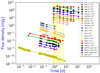 |
Fig. 1. GRB 160131A light curves from radio to X-rays. Yellow shaded areas show the time intervals (centred to 0.8 d, 1.7 d, 2.7 d, and 5.8 d) where SEDs have been empirically analysed. Filled circles indicate detections (uncertainties are smaller than the corresponding symbol sizes), which are connected with each other through a segment, and upside down triangles indicate 3σ upper limits. |
To investigate the relation between radio and optical/X-rays, we linearly (in a log–log plot) interpolated data (Fig. 2, red points) at those epochs, where needed.
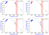 |
Fig. 2. Broadband SEDs of GRB 160131A at 0.8 d (top left), 1.7 d (top right), 2.7 d (bottom left), and 5.8 d (bottom right). Blue (red) points are measured (linearly interpolated in a log-log plot) data. These SEDs display radio peaks (at 0.8 d, 1.7 d, and 5.8 d) and dust extinction (red shaded regions, especially at 0.8 d). The green dashed line shows the resulting modelling of the high-energy data (optical/X-ray). Filled circles indicate detections, and upside-down triangles indicate 3σ upper limits. |
The high-energy side of the SEDs (Fig. 2) is well-fitted by a power law with a mean value of βhe = −1.09 ± 0.0418, corresponding to a photon index Γ = 1 − βhe = 2.09 ± 0.04, compatible with ΓX obtained from XRT data (Sect. 2.1). This constrains the behaviour of the break frequencies (especially νc and νm), as well as the possible jet break, the time evolution of the blastwave, and the kind of environment (ISM vs. wind).
4.2. Optical/X-ray data set: νm – νc location, CBM density profile, and jet break
As we can see in Fig. 3, the optical/X-ray fluxes decay with temporal index αhe ∼ −1.25 up to ∼0.1 d, followed by a plateau (more pronounced in the optical data) in the temporal range ∼0.1–0.8 d (αX, ei ∼ −1), possibly suggesting energy injection (Sect. 5.1); after the plateau, the flux decay steepens to αhe ∼ −1.8 and can be interpreted in terms of a jet break (Sect. 4.3.2).
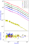 |
Fig. 3. Light curves for GRB 160131A of visible and X-ray data modelled with DBPL (Eq. (4)). We observe the plateau, probably ascribable to the energy injection between ∼104 and ∼7 × 10⁴ s (∼0.1 and 0.8 d), and the achromatic break at ∼9 × 10⁴ s (∼1 d), typical of jetted emission. Bottom panel: residuals of the fit. |
In the context of the standard afterglow model, the absence of any break frequencies between optical and X-ray domains suggests that νm and νc must lie either below or above the optical/X-ray frequencies νopt, X at the first epoch of observations tobs, 0 (∼10−3 d). In the following, we explore the different possibilities:
Fast cooling regime.νopt, X < νc < νm is incompatible with this regime because the optical/X-ray spectra are expected to show only positive values of β (1/3 ≲ β ≲ 2 for any possible spectrum). Moreover, νc < νopt, X < νm is incompatible with this regime because the optical/X-ray spectra are expected to show β ∼ −0.5 instead of the observed βhe = −1.08. Finally, the case where νc < νm < νopt, X is compatible with the fast-cooling regime because, following the indices α and β calculated for different spectral regimes in GS02, it requires an electron energy index of p = −2βhe ∼ 2.18 and a decay rate of α = (2 − 3p)/4 ∼ −1.14 (regardless of the CBM), compatible with αhe; this suggests that νm is just below optical frequencies at tobs, 0.
Slow cooling regime.νopt, X < νm < νc is incompatible with this regime because the optical/X-ray spectra are expected to show only positive values of β (1/3 ≲ β ≲ 2 for any possible spectrum). Moreover, νm < νopt, X < νc is incompatible with this regime because it requires p = 1 − 2βhe ∼ 3.18 and α ∼ −1.64 for an ISM-like CBM (α ∼ −2.14 for a wind-like CBM) in GS02, which is too steep for real light curves. Finally, the case where νm < νc < νopt, X is compatible with the slow-cooling regime, because it requires p = −2βhe ∼ 2.18 and α = (2 − 3p)/4 ∼ −1.14 (the same regime as the fast-cooling case), suggesting that νm is well below optical frequencies at tobs, 0.
This picture constrains νm and νc below νopt = 3 × 10¹⁴ Hz at tobs, 0. Moreover, the absence of any break in these light curves until ∼0.1 d (after which energy injection and jet break occur) suggests a decreasing evolution of νc, which favours an ISM-like CBM over a wind-like CBM in the standard afterglow model.
From the upper limit on νopt and using the temporal scaling for both νm (t−3/2) and νc (t−1/2 for ISM), we constrain the passage of νm and νc in the radio frequencies. The passage of νm is constrained in Ka-band at tobs < 2.1 d, in K-band at tobs < 2.8 d, in Ku-band at tobs < 3.6 d, in X-band at tobs < 4.7 d, and in C-band at tobs < 6.7 d. Moreover, νc is expected to cross the radio domain at late-time (Ku-band at tobs < 4 × 10⁵ d), and therefore be virtually unobservable.
Assuming the classical results by Sari et al. (1999), the decay of the light curve after the break (tj ∼ 1 d) is −p for νm < ν < νc and ν > νc (corresponding to our picture). This post-jet decay (αpost, j = −p ∼ −2.2) is steeper than expected for the optical/x-ray decay (αhe ∼ −1.8), and hence we assume a milder jet break model (pure edge effect, Sect. 3.2), characterised by a post-jet decay αpost, j = αpre, j − (3 − k)/(4 − k) (Granot 2007): assuming ISM-like CBM (and hence k = 0), we obtain αpost, j = −1.25 − 0.75 = −2, which is compatible with the observed value (α ∼ −1.8).
In summary, the optical/X-ray data suggest that (1) the CBM is preferably described by ISM, (2) the transition between fast and slow cooling regime is not constrained by optical/X-ray observations, (3) p ∼ 2.2, (4) both νm and νc lie below νopt = 3 × 10¹⁴ Hz already at tpost, 0, and (5) a milder jet break model (pure edge effect) is in accordance with the optical/X-ray data. A more accurate identification of the break frequencies requires a comprehensive data analysis within a self-consistent broadband modelling (Sect. 4.4).
4.3. Data set from the Very Large Array
We analyse both the radio SEDs at each epoch from 0.8 d to 117 d and the light curves from 4.6 GHz to 37.4 GHz.
4.3.1. Radio SEDs: the νsa location and the multi-component approach
One of the most impressive features in radio SEDs is the presence of spectral bumps or peaks at several epochs (Fig. 4, red circles). We preliminarily modelled these radio SEDs ignoring the peaks with either a power law or a broken power law (Fig. 4) in order to compare the resulting spectral indices with those expected from the synchrotron emission of GRB afterglows. We then analysed the radio SEDs including the whole data set in a multi-component approach (Fig. 5):
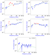 |
Fig. 4. Radio SEDs of GRB 160131A from 0.8 to 44.8 d. Top left: data together with a BPL (Eq. (3)) at 0.8 d; red points identify the bump and were ignored by the fit. Top right: radio SED at 2.7 d fitted with a BPL. Middle left: data together with an empirical SPL (Eq. (2)) at 5.8 d; red points identify the bump ∼8 GHz and were ignored by the fit. Middle right: radio SED at 12.7 d fitted with a BPL. Bottom: data together with a BPL (Eq. (3)) at 44.8 d. Green dashed lines show the resulting modelling. Filled circles indicate detections, and upside-down triangles indicate 3σ upper limits. |
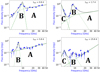 |
Fig. 5. Radio SEDs of GRB 160131A from 0.8 to 25.8 d in a multi-component approach. Top left: data together with the sum of two BPLs at 0.8 d. Top right: radio data at 1.7 d together with the sum of a SPL and two BPLs. Bottom left: data together with the sum of a SPL and a BPL at 5.8 d. Bottom right: radio SED at 25.8 d fitted with the sum of a SPL and two BPLs. Black lines show the resulting modelling, and green dash-dotted or dotted lines indicate each component. Filled circles indicate detections, and upside-down triangles indicate 3σ upper limits. |
– 0.8 d radio SED. This SED shows a peak at ∼9 GHz and width Δν ∼ 2 GHz (Fig. 4, top left). Neglecting this peak, this SED is described by a BPL (Eq. (3); Table 2). The constraints on νm described in Sect. 4.2 suggest that for this epoch νm < 150 GHz; the comparison between the values of β shown in Table 2 and in Fig. 1 of GS02 suggests that νsa crossed the radio band in the slow-cooling regime (scenario 1, νsa < νm < νc, GS02). Unfortunately, the presence of the extra-component peaking at ∼9 GHz prevents us from better constraining νsa.
– 2.7 d radio SED. This SED is characterised by a broad peak at ∼25 GHz, which can be modelled with a BPL (Eq. (3); Fig. 4, top right; Table 2). The constraints described in Sect. 4.2 suggest that for this epoch νm < 22 GHz. This SED is compatible with the slow-cooling regime (scenario 1, νsa < νm < νc, GS02): β2, bpl in Table 2 is steeper than 1/3 for this regime, suggesting a probable proximity between νb ∼ νm and νsa.
– 5.8 d radio SED. This SED, characterised by a strong and narrow peak at ∼7 GHz, is modelled with a SPL (Eq. (2); Fig. 4, middle left; Table 2); for this epoch, νm < 7.3 GHz (Sect. 4.2) suggests the slow-cooling regime, but the value of β is incompatible with regimes described in the standard afterglow model.
– 12.7 d radio SED. This SED, showing a peak at ∼7 GHz, can be modelled with a BPL (Eq. (3); Fig. 4, middle right; Table 2). At this epoch, we expect that νm < 2.3 GHz (Sect. 4.2), and so this behaviour is compatible with the slow-cooling regime (scenario 2 of GS02, νm < νsa < νc), where νsa = νb, β1, bpl = 2.5, and β2, bpl = (1 − p)/2 (suggesting p = 2.04 ± 0.10).
– 44.8 d radio SED. This SED is similar to the 12.7 d one, except that it is dimmer. It can be modelled with a BPL (Eq. (3); Fig. 4, bottom; Table 2). At this epoch, it is νm < 0.35 GHz (Sect. 4.2), and therefore this behaviour could still be compatible with the slow-cooling regime (scenario 2), although β2, bpl is steeper than expected; in this scenario, νsa = νb, β1, bpl = 2.5, and β2, bpl = (1 − p)/2 (suggesting p = 2.1 ± 0.6).
The relatively large uncertainties on flux density in the SEDs at ν ≲ 6 GHz inevitably affect the ability to constrain νsa. Assuming νb ∼ νsa in the radio SEDs at 0.8 d and 12.7 d (Table 2), we obtain that νsa could evolve approximately as t−0.1, with is compatible with νsa being constant over time, as expected for the ISM (GS02).
Now including the peaks in the radio SEDs, we consider the whole radio data set in a multi-component approach. In addition to the continuum associated with FS emission (Sect. 4.3.1, hereafter component A), radio SEDs suggest a further two distinct emission components (Fig. 5).
Component B appears at four epochs (0.8, 1.7, 5.8, and 25.8 d) and is characterised by a faint peak around 9 GHz (Fig. 5). We fit this component with a BPL, obtaining the results shown in Table 3.
Component C shows up in the 25.8 d radio SED, and partially appears at 1.7 d (Fig. 5), when the lack of radio data at ≲5 GHz does not allow us to resolve its peak. We fit this component with a SPL (1.7 d) and a BPL (25.8 d), obtaining the results shown in Table 3.
In the multi-component approach, we briefly focus on the radio SED at 1.7 d (Fig. 5, top right), which is well-fitted by a combination of a SPL at ≲5 GHz (a possible part of the component C) and a BPL peaking at ∼9 GHz (component B, Table 3). As opposed to the other SEDs, the absence of data at high frequencies prevents us from constraining component A which is associated with the FS emission of GRB afterglow. In Fig. 5 (top right), we add the component A to a BPL characterised by the same spectral indices as those seen in the 0.8 d radio SED, and a flux density of 0.1 mJy (Table 3).
In summary, the radio SEDs suggest that (1) the slow-cooling regime occurs at t ≲ 0.8 d, (2) at 5.8 d the features are incompatible with the standard GRB afterglow model, (3) at 12.7 d νsa ∼ 7 GHz, and that (4) the radio data set is composed of three spectral components (A, B, and C), of which only the first one (A) is connected with a known physical effect (the continuum associated with FS emission). We explore these components further in Sect. 5.
4.3.2. Radio light curves: evidence for a jet
Radio data help to constrain both the FS emission and the jet opening angle. In this context we analysed the radio light curves whilst ignoring the peaks ascribed to additional components (Sect. 4.3.1) as well as data below 8 GHz because of the high variability, which is probably caused by strong ISS (Sects. 5.2 and 3.2), which prevents further constraint of the rise and decline rates.
In the standard afterglow model, a jet break arises at the time tj when the bulk Lorentz factor Γ decreases below the inverse opening angle of the jet  and its edges become visible to an observer (Sect. 3.2). Once νm has crossed the observing frequency, the flux density decays steeply following a jet break. In this regime, the steepening in the radio light curves is expected to follow that of the steepening in the optical/X-ray light curves, depending on the time it takes for νm to cross the radio band (Laskar et al. 2015). The identification of νb ∼ 23 GHz with νm observed in the SED at tobs = 2.7 d (Fig. 4 and Table 2) indicates that the light curve at νobs ∼ νb would peak at tobs. We observed this behaviour in the light curve at 24.6 GHz (Fig. 6, middle left), which is well fitted by a BPL (Eq. (3)); the best-fit results (Table 4) show that α2, bpl is also compatible with αhe obtained for optical/X-ray light curves (Sect. 4.2), and therefore with the passage of νm in the light curves of standard GRB afterglow model (Sari et al. 1998). The radio light curves above 24.6 GHz show a steep decay of the flux densities at tb ranging between ∼3 and ∼5 d, compatible with jet break; modelling with BPL (Eq. (3)) shows −0.1 ≲ α1 ≲ 0.1 and −2 ≲ α2 ≲ −1.6 (Fig. 6, middle left and bottom; Table 4). At t = tj ∼ 1 d, as inferred from optical/X-ray light curves, νm lies close to ∼1011 GHz, which is well below the optical/X-ray domain. This is consistent with the steep decline observed around the same epoch in these bands.
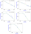 |
Fig. 6. Radio light curves of GRB 160131A in the range 9 − 37 GHz. 8.93 GHz (top left) and 11.4 GHz (top right) fitted with a SPL (Eq. 2); the other light curves (24.6 GHz, middle left; 30.4 GHz, middle right; 37.1 GHz, bottom) are fitted with a BPL (Eq. (3)). Blue filled circles indicate detections, and upside-down triangles indicate 3σ upper limits; red circles indicate the ignored points corresponding to the peaks observed in radio SEDs (Fig. 4), and green lines show the resulting model. |
For completeness, we obtained further information about break frequencies of synchrotron emission from the decreasing temporal decay indices α in the light curves between 8 GHz and 24.6 GHz. In particular, the value α ∼ −0.6 (Table 4) obtained by modelling the light curves between 8 GHz and 14 GHz (Fig. 6, top left and top right) with a SPL (Eq. (2)) suggests that –in agreement with what was inferred from the high-energy data analysis (Sect. 4.2)– (1) νc crosses these frequencies after 45 d and (2) the passage of νm occurs at t ≲ 3 d (Sari et al. 1998). Furthermore, the decreasing temporal indices in the light curves between 14 GHz and 24.6 GHz, evolving from ∼ − 0.8 at 14 GHz to ∼ − 1.2 at 24 GHz, are suggestive of the passage of νc in these light curves above ∼120 d, and the passage of νm at these observing frequencies is very close to 3 d (Sari et al. 1998).
4.4. Physical approach: modelling with SAGA
The complexity of the broadband spectral and temporal properties, in particular the spectral radio peaks (Fig. 2), means that an iterative analysis (optical, optical/X-ray, optical/X-ray/radio) is necessary to probe the physical characteristics of the afterglow of GRB 160131A, and that the broadband model of GRB afterglow needs to be overseen in order to determine when it starts losing validity. We considered in this analysis a jetted (edge-regime) FS emission with dust extinction and energy injection in an ISM-like CBM; we also considered the ISS effect, which is typical of the radio domain, following the procedure described in Misra et al. (2021). The modelling ignored the data at tobs < T90 = 4 × 10⁻³ d, where the prompt emission has not yet subsided.
From the analysis reported in Sects. 4.2 and 4.3, we adopted the following values as starting points for the micro-physics parameters (Sect. 3.2 and Table 1): p = 2.2, ϵB = 0.01, n0 = 1 cm−3, Ek, iso, 52 = 50, AV = 0.1, tj = 1 d, and m = 0.2. Moreover, according to a method that has been used in the past to constrain ϵe through the identification of the radio peaks (observed in the radio light curves) connected with the passage of νm (Beniamini & van der Horst 2017), we used the peak (with a flux density F ∼ 0.9 mJy) observed in the 24.6 GHz light curve at tobs ∼ 3 d (Sect. 4.3.2) to estimate ϵe ∼ 0.1 as a starting point.
4.4.1. From optical to X-rays
The iterative process of modelling from 3 × 10¹⁴ to 6.6 × 10¹⁷ Hz shows a good best-fit model ( ∼ 1; see results in the first two columns of Table 5), as displayed in the broadband light curves (Fig. 7 for optical frequencies, and Fig. 8 for optical/X-ray domain).
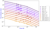 |
Fig. 7. Broadband modelling (UVOIR frequencies; Table 5, first column) of GRB 160131A for a FS model with a ISM-like CBM (GS02); we considered in this analysis a jetted (edge-regime) emission with dust extinction and energy injection. Filled circles indicate detections, and downward triangles indicate 3σ upper limits. |
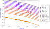 |
Fig. 8. Broadband modelling (from optical to X-ray frequencies; Table 5, second column) of GRB 160131A. See the caption of Fig. 7 for a full description of the modelling. Filled circles indicate detections, and downward triangles indicate 3σ upper limits. |
Summary statistics from MCMC analysis obtained with SAGA applied to the visible and UV data of GRB 160131A for a model based on a jetted (edge-regime) FS emission with optical absorption and energy injection, in an ISM-like CBM.
Our results (Table 5) show that the spectrum is in the fast-cooling regime until ttrans ∼ 0.02 d and the NR regime occurs at ∼300 d; the cooling due to IC scattering is negligible because of the very low Compton y-parameter (0.02).
SAGA also estimates the behaviour of the synchrotron break frequency over time (Fig. 9). With reference to the lines of reasoning put forward in Sect. 4.2 (βhe = −1.09 suggests that νm and νc must lie in the same spectral regime below νopt, X at tobs, 0 ∼ = 10−3 d), the temporal evolution of νc and νm is in accordance with SAGA results (Fig. 9). On the other hand, with reference to the arguments proposed in Sect. 4.3.2 (radio SEDs suggest that νsa ∼ 7 GHz until tobs ∼ 13 d), the temporal evolution of νsa (Fig. 9) is incompatible with SAGA results (νsa ∼ 100 GHz at tobs ∼ 13 d), which is due to the lack of radio data in the optical/X-ray analysis.
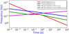 |
Fig. 9. Temporal evolution of the synchrotron break frequencies for afterglow emission of GRB 160131A, based on analysis of UVOIR/X-ray data (Table 5, second column). See the caption of Fig. 7 for a full description of the modelling. The self-absorption frequency produced by noncooled electrons νac makes sense only in fast-cooling regime (≲0.02 d). |
For completeness, Fig. 10 shows the light curves in the UVOIR/X-rays domain at four observing frequencies (i′-filter, top left; g′-filter, top right; UV/uvw1-filter, bottom left; and X-ray frequency, bottom right), and Fig. 11 shows all the radio data (dashed lines, not included in this part of the modelling) with the predicted SEDs in this domain obtained from modelling the optical/X-ray data; these data do not match the high-energy sample, as we show and discuss in the following section.
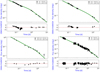 |
Fig. 10. Light curves of GRB 160131A in the UVOIR/X-rays domain at i′-filter (4.03 × 10¹⁴, top left), g′-filter (6.47 × 10¹⁴, top right), UV/uvw1-filter (1.15 × 10¹⁵, bottom left), and X-ray frequency (6.65 × 10¹⁷, bottom right), referred to the broadband modelling from optical to X-ray frequencies (Table 5, second column), displayed in Fig. 8. The bottom panel of each light curve corresponds to the residuals of the fit. See the caption of Fig. 7 for a full description of the modelling. Filled circles indicate detections, upside down triangles indicate 3σ upper limits, and green lines show the resulting model. |
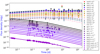 |
Fig. 11. Broadband modelling (from optical to X-ray frequencies; Table 5, second column) of GRB 160131A. See the caption of Fig. 7 for a full description of the modelling. Filled circles indicate detections, and downward triangles indicate 3σ upper limits. For completeness we include all the radio data (dashed lines, not modelled in this approach) and relative light curves (derived from optical/X-ray modelling). |
4.4.2. From radio to X-ray frequencies
The radio/mm data set from 0.6 to 92.5 GHz does not include the data points affected by the bumps (Sect. 4.3), because the best-fit model with the whole radio data set was very poor ( > 30). To verify the stability and robustness of the best-fit solution, we repeated the analysis assuming three different starting values for p (2.1, 2.4, 2.9); we obtained p ∼ 2, which is lower than that estimated from the high-energy approach (Sect. 4.2), but is compatible with the analysis of the radio SEDs in the empirical approach (Sect. 4.3.1). The poor modelling of these three analyses (
 > 20) led us to consider a fixed value for p (2.2, according to the high-energy approach; Sect. 4.2) as a compromise.
Unsurprisingly, the best-fit model has a very high  (∼10; Table 5, third column). This is indicative of the problems faced by the standard GRB afterglow model, which are common in cases where a rich data set at low frequencies is available (Fig. 12).
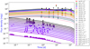 |
Fig. 12. Broadband modelling of GRB 160131A from radio to X-ray frequencies (Table 5, third column). See the caption of Fig. 7 for a full description of the modelling. Filled circles indicate detections, and downward triangles indicate 3σ upper limits. |
Our results (Table 5, third column) show that the jet break time of 0.9 d translates into a jet opening angle θj ∼ 8 degrees, ttrans ∼ 9 × 10⁻⁵ d, and the NR regime occurs at ∼120 d. Moreover, Fig. 12 shows that the model is only suitable for radio (except for ν ≲ 10 GHz) domains, and is only partially suited to X-ray frequencies and is poorly suited to the optical band. This behaviour suggests that other radiation mechanisms are responsible for the afterglow emission for GRB 160131A. As in the case of the analysis of optical/X-ray data (Sect. 4.4.1), the Compton y-parameter is 0.02, indicating that cooling due to IC scattering is negligible. The temporal evolution of the cooling frequency νc (Fig. 13) suggests that it lies above the X-rays (as opposed to νsa and νm), in contrast with the behaviour expected from empirical considerations based on the optical/X-ray spectra (Sect. 4.2).
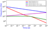 |
Fig. 13. Temporal evolution of the synchrotron break frequencies for afterglow emission of GRB 160131A based on analysis of broadband data (from radio to X-ray frequencies; Table 5, third column). See the caption of Fig. 7 for a full description of the modelling. The self-absorption frequency produced by non-cooled electrons νac only makes sense in the fast-cooling regime (≲9 × 10⁻⁵ d). |
5. Discussion
The addition of radio data set in the afterglow modelling considerably complicates the broadband analysis, challenging the standard GRB afterglow model.
We point out three problematic features at radio frequencies:
1. The presence of the same rather constant peak at ∼8 GHz in SEDs up to ∼25 d, whose width Δν/ν evolves from ∼0.5 at 1.7 d to ∼0.1 at ∼25 d, with a temporary disappearance at ∼2.7 d (Fig. 4).
2. The SED at 5.8 d evolves with β ∼ 0.7 (Table 2 and Fig. 4), a value which is incompatible with slow cooling regimes for FS emission (Sect. 4.2).
3. Flux densities at low frequencies (≲7 GHz) seem to be constant over time (Figs. 4 and 5).
Our results suggest that radio data cannot be fully accounted for alongside the optical/X-ray data within the framework of the standard GRB afterglow model. This is not unprecedented: for example, Kangas & Fruchter (2021) reported a lack of detectable jet breaks in the radio light curves of a sample of 15 GRB afterglows, whereas X-rays seem to support them. However, we underline that these latter authors (1) considered only one spectral regime (5-1-2) of afterglow emission in GS02, (2) assumed the sideways expansion for jetted emission, and (3) ignored any observed rise period of the light curve and any early features attributed to flares, plateau, or RS in the literature. They interpret the long-lasting single power-law decline of the radio emission in terms of a two-component jet.
There are other possible assumptions that might not necessarily hold true for the afterglow of GRB 160131A: (1) the constant micro-physics parameters, in light of the evidence of the temporal evolution of the micro-physics parameters in the afterglow of GRB 190114C (Misra et al. 2021), (2) a unique CBM, as in the case of evidence of the transition from a wind-like to ISM-like CBM in the afterglow of GRB 140423A (Li et al. 2020), and (3) a uniform jet model, in light of the evidence of other jet models used to interpret the broadband data for several GRB afterglows, such as the structured jet model (e.g. De Colle et al. 2012; Granot et al. 2018; Alexander et al. 2018; Coughlin & Begelman 2020), a two-component jet (e.g. Berger et al. 2003; Peng et al. 2005; Racusin et al. 2008; Liu & Wang 2011; Holland et al. 2012) and other more complex regimes (e.g. Huang et al. 2004; Wu et al. 2005; Granot et al. 2018). In recent years, growing evidence has been found in favour of the structured jet19, as in the case of the GRB 170817A associated to GW 170817 (Alexander et al. 2018).
5.1. Energy injection
A flattening in the optical/X-ray light curves prior to 0.8 d of GRB 160131A could demand energy injection. Nothing can be inferred in this regard from radio data, which were taken starting from ∼1 d.
In the energy injection approach (Sect. 3.2), the inferred value p ∼ 2.2 (Sect. 4) suggests νc < νX, where the flux density is  (GS02); in this regime we obtain
  . The temporal evolution of the injected energy is parameterised as E ∝ tm, and hence Fν > νc ∝ t1.1m − 1.3. Fitting the X-ray light curve with a power law from ∼0.2 d to ∼0.8 d, which roughly corresponds to the flattening, we obtain αX, ei = −1.0 ± 0.2; apparently, this temporal decay index does not require that an energy injection effect being added in the modelling, but the addition of the UVOIR data set in the broadband modelling necessarily invokes this effect. In the energy injection approach, the value of αX, ei implies m = 0.27 ± 0.20, or, equivalently, q = 1 − m = 0.73 ± 0.20. This conclusion is perfectly compatible with our optical/X-ray modelling (Sect. 4.4.1 and Table 5, first and second column), where we adopted the energy injection approach (Sect. 3.2); in particular, we obtained an increasing Ek, iso, 52 from ∼4.2 × 1053 erg to ∼4.9 × 1053 erg (Fig. 14). A similar energy injection process was discussed for GRB 100418A, for which m ∼ 0.7 was found (Marshall et al. 2011; Laskar et al. 2015).
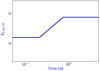 |
Fig. 14. Isotropic equivalent kinetic energy Ek, iso, 52 (in units of 1052 erg) as a function of time, as determined from modelling of the optical/X-ray data set (Table 5, second column). |
As we can see in Fig. 3, the X-ray light curve shows a less pronounced flattening with respect to optical light curves. This unusual light curve was also observed with GRB 090102 (Gendre et al. 2010), where the optical flattening could then be interpreted as (1) a change of the CBM (e.g. Ramirez-Ruiz et al. 2001; Chevalier et al. 2004), and (2) a normal fireball expanding in an ISM, with a RS component (the lack of radio data does not corroborate this assumption). Another similar feature is present in GRB 060908 (Covino et al. 2010), where it is possible to model the optical and X-ray afterglows independently, but the multi-frequency spectral and temporal data challenge available theoretical scenarios. The broadband modelling of the afterglow of the ultra-long duration GRB 111209A (Kann et al. 2018) shows a strong chromatic rebrightening in the optical domain, which is modelled with a two-component jet; the late afterglow also shows several smaller, achromatic rebrightenings, which are likely to be energy injections.
5.2. The possible role of ISS in the multi-component radio SEDs
The evidence of the multi-component SEDs at radio frequencies (A, B, and C; Sect. 4.3.1) suggests further radiation mechanisms for the GRB afterglow in addition to the continuum associated with FS emission.
The presence of peaks in radio SEDs had already been observed in other sources, and the main candidate to explain this pronounced radio variability is the ISS (or other extreme scattering effects); in particular, the VLA SED at ∼2 d of GRB 130925A (Horesh et al. 2015) shows a peak at ∼8 GHz, with Δν/ν ∼ 0.7, compatible with our values (Δν/ν ∼ 0.1 − 0.5, as observed in Sect. 5). Horesh et al. (2015) suggest that these peaks are well modelled with the ISS emission model in which the emission originates from either mono-energetic electrons or an electron population with an unusually steep power-law energy distribution. Moreover, thanks to a simple modelling of the radio data set with SAGA, we obtained SEDs (Fig. 15) and light curves (Fig. 16) that are well modelled with the expected variability due to the ISS effect (red shaded regions).
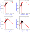 |
Fig. 15. Radio SEDs of GRB 160131A at 0.8 d (top left), 1.7 d (top right), 5.8 d (bottom left), and 25.8 d (bottom right), obtained through a radio modelling for a FS model in ISM; we considered a jetted (edge-regime) emission with ISS effect. Filled circles indicate detections, and upside down triangles indicate 3σ upper limits; the red shaded regions represent the expected variability due to ISS effect, obtained through the prescription described in Misra et al. (2021). |
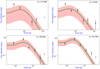 |
Fig. 16. Radio light curves of GRB 160131A at 11.4 GHz (top left), 13 GHz (top right), 18.8 GHz (bottom left), and 24.6 GHz (bottom right), obtained through a radio modelling (from radio to X-ray frequencies) for a FS model in ISM; we considered a jetted (edge-regime) emission with ISS effect, dust extinction and energy injection. Filled circles indicate detections, and upside-down triangles indicate 3σ upper limits; the red shaded regions represent the expected variability due to the ISS effect obtained through the prescription described in Misra et al. (2021). |
Another interpretation for this radio excess at early times is that it should have been ascribable to the presence of a RS in addition to a FS (e.g. Gomboc et al. 2008; Melandri et al. 2010; Japelj et al. 2014; Alexander et al. 2017; Laskar et al. 2018a), because (1) the RS emission is expected to peak at lower frequencies than the FS, and (2) the RS spectrum is expected to cut off steeply above the RS cooling frequency (Kobayashi & Sari 2000). A recent study (Laskar et al. 2019b) showed for the first time that within a SED it is possible to disentangle the contributions of RS and FS in the radio band. Moreover, the first case of a SED instantaneously and clearly decomposed into RS and FS components (GRB 181201A, Laskar et al. 2018b) suggests that an early-time radio peak is consistent with emission from a refreshed RS produced by the violent collision of two shells with different Lorentz factors emitted at different times. Nevertheless, the peak at lower frequency bands observed in the radio SEDs of Laskar et al. (2019b), which is characterised by Δν/ν ∼ 3, is much broader than what we find (Δν/ν ∼ 0.1 − 0.5, as observed in Sect. 5), calling for something else that comes into play in addition to the RS prescription. This incompatibility is strengthened by the lower limit on n0 estimated with SAGA (n0 ≳ 5 cm−3) and the strong observed correlation –highlighted in several analyses (e.g. GRB 160509A in Laskar et al. 2016a, GRB 161219B in Laskar et al. 2018a, and GRB 181201A in Laskar et al. 2019b)– between broadband detections of RS emission and CBM characterised by low densities (typically n0 ≲ 10−2 cm−3 in ISM-like CBM, and A* ≲ 10−2 in wind-like CBM). In hindsight, these features could have possibly been observed in more sparse radio data sets from past GRBs as well, and erroneously interpreted as evidence of a RS.
We further rule out the presence of RS emission by analysing these peaks in the radio SEDs according to the prescription taken up by Laskar et al. (2018b). These authors assume νc, rs to be located near each observed radio spectral peak in order to compute a conservative lower limit to the optical light curve20. At radio frequencies, the first spectral peak takes place at F ≈ 0.9 Jy in X-band (∼9 GHz) at 0.8 d (Fig. 4); following the reasoning behind the evolution of νc, rs, we assume νc, rs ≈ 9 GHz and Fν, pk ≈ 0.9 Jy at this epoch.
– In the relativistic RS regime, the Y-band (∼3 × 10¹⁴ Hz) would be crossed by a relativistic RS (ISM) at tpk ∼ 8.5 × 10⁻⁴ d with Fν, pk ∼ 730 Jy (tpk ∼ 3.1 × 10⁻³ d and Fν, pk ∼ 465 Jy for wind). Unfortunately, there are no optical data at those epochs, and therefore we scale Fν, pk at tpk knowing that the observed Y-band light curve evolves as ∼t−1.25 (Sect. 4.2), obtaining Fν, pk ∼ 920 Jy for ISM-like CBM (Fν, pk ∼ 180 Jy at ∼3.1 × 10⁻³ d for wind-like CBM), which is incompatible with the relativistic RS regime.
– In the Newtonian RS approach, for the same spectral peak we obtain the passage of νc, rs in Y-band (1) in the range ≈(1.7 − 0.5)×10−3 d (corresponding to Fν, pk ∼ 450 − 728 Jy) for an ISM-like CBM, and (2) in the range ≈(8.6 − 1.7)×10−3 d (corresponding to Fν, pk ∼ 260 − 450 Jy) for a wind-like CBM. In this case, there are also no optical data at those epochs to verify this assumption; the observed Y-band light curve evolves as ∼ − 1.25, resulting in Fν, pk ∼ 390 − 1930 Jy for an ISM-like CBM (Fν, pk ∼ 50 − 390 Jy for wind-like CBM); this behaviour seems to be compatible with the predicted Y-band light curve.
The radio peak clearly observed in the 1.7 d SED at the same frequency (Fig. 5, top right) is incompatible with the temporal evolution of νc, rs for RS emission because, considering the observed peak at ∼9 GHz in the 0.8 d-radio SED, at 1.7 d we would observe νc, rs ∼ 3 GHz in an ISM-like CBM (νc, rs ∼ 2 GHz in wind-like CBM); this suggests that the RS is unlikely to play a dominant role in radio data for GRB 160131A.
Other possible explanations for the radio spectral bumps could be (1) a two-component jet, one in which the optical/X-ray emission arises from a narrower, faster jet than that producing the radio observations (i.e. Peng et al. 2005; Racusin et al. 2008; Holland et al. 2012), or (2) the presence of a population of thermal electrons not accelerated by the FS passage into a relativistic power-law distribution (Eichler & Waxman 2005), and characterised by a much lower Lorentz factor than the minimum Lorentz factor of the shock-accelerated electrons (‘cold electron model’; Ressler & Laskar 2017).
6. Conclusions
We present our results on the broadband modelling of the afterglow of GRB 160131A, whose observations span from ∼330 s to ∼160 d post explosion at 26 frequencies from 6 × 10⁸ Hz to 7 × 10¹⁷ Hz.
In the data modelling we consider a jetted (edge-regime) FS emission with energy injection, the ISS effect, dust extinction, and absorption effects in ISM-like CBM. Our analysis of the UVOIR/X-ray data alone leads us to the following results: p ∼ 2.2, ϵe ∼ 0.01, ϵB ∼ 0.1, n0 ≳ 10 cm−3, EK, iso ≳ 5 × 1053 erg, AV ∼ 0.2 mag, and tj ∼ 0.9 d. The constraint on tj leads to an estimate of the jet half opening angle of θj ∼ 6°, corresponding to a beaming-corrected kinetic energy of the explosion EK = EK, iso(1 − cos θj)≳3 × 1051 erg, in agreement with the typical values of long GRBs (Figs. 21 and 22 of Laskar et al. 2015). The spectrum is in fast cooling until ∼0.02 d, the non-relativistic regime sets in at ∼100 d, and the energy injection is characterised by m ∼ 0.15. The radio data set –which in this case is particularly rich– shows the presence of spectral bumps in several SEDs, which are incompatible with a simple standard GRB afterglow model and probably ascribable to either ISS (or other extreme scattering effects) or a more complex multi-component structure. This incompatibility is corroborated by the broadband modelling from radio to high energies, where the model works well for the radio domain (except for ν ≲ 10 GHz), but not quite as well at X-ray frequencies, and poorly for the optical band. Our conclusions challenge the standard GRB afterglow model; moreover, these results highlight the as-yet poorly understood physics, especially when a rich data set (from radio to high-energy domain) – as in the case of GRB 160131A – is included in the modelling.
Future broadband follow-up studies of GRB afterglows, particularly at radio frequencies with the latest and forthcoming generation facilities –especially in interferometric mode– such as the Very Large Baseline Array (VLBA21), LOw Frequency ARray (LOFAR, van Haarlem et al. 2013) or the next generation Square Kilometer Array (SKA; Johnston et al. 2008), are essential in order to reach an exhaustive comprehension of the GRB afterglow physics, particularly within the modern era of multi-messenger astronomy.
Derived using https://www.swift.ac.uk/analysis/nhtot/, taking the value NH, tot.
This jet regime is simpler than structured jet model, that assumes an angular distribution in energy and Lorentz factor, based on special relativistic hydrodynamics (e.g. De Colle et al. 2012; Granot et al. 2018; Coughlin & Begelman 2020), and other more complex regimes (e.g. Huang et al. 2004; Peng et al. 2005; Wu et al. 2005; Granot et al. 2018).
The same approach is sometimes based on L(t) = L0(t/t0)q and q ≤ 0 (e.g. Misra et al. 2007; Marshall et al. 2011; van Eerten 2014; Laskar et al. 2015).
Recently, the open-source Python package AFTERGLOWPY became available for on-the-fly computation of structured jet afterglows with arbitrary viewing angle (Ryan et al. 2020).
Acknowledgments
We thank the anonymous referee for helping us improve the paper. Support for this work was provided by Università degli Studi di Ferrara through grant FIR 2018 “A Broad-band study of Cosmic Gamma-Ray Burst Prompt and Afterglow Emission” (PI Guidorzi). M. Marongiu acknowledges financial support from the Italian Ministry of University and Research – Project Proposal CIR01_00010, and the University of Ferrara for the financial support of his PhD scholarship (during the data analysis and the interpretation of the results). M. Marongiu is very grateful to R. Martone for useful conversations about GRB science; moreover, M. Marongiu thanks P. Bergamini and G. Angora for the useful discussion about Python programming language and data analysis. A. Gomboc acknowledges the financial support from the Slovenian Research Agency (grants P1-0031, I0-0033, J1-8136, J1-2460) and networking support by the COST Actions CA16104 GWverse and CA16214 PHAROS. N. Jordana and C.G. Mundell acknowledge financial support from Mr Jim Sherwin and Mrs Hiroko Sherwin. D. Kopac acknowledges the financial support from the Slovenian Research Agency (research core funding No. P1-0188). The National Radio Astronomy Observatory is a facility of the National Science Foundation operated under cooperative agreement by Associated Universities, Inc..
References
- Abbott, B. P., Abbott, R., Abbott, T. D., et al. 2017, ApJ, 848, L12 [Google Scholar]
- Aksulu, M. D., Wijers, R. A. M. J., van Eerten, H. J., & van der Horst, A. J. 2020, MNRAS, 497, 4672 [NASA ADS] [CrossRef] [Google Scholar]
- Alexander, K. D., Laskar, T., Berger, E., et al. 2017, ApJ, 848, 69 [NASA ADS] [CrossRef] [Google Scholar]
- Alexander, K. D., Margutti, R., Blanchard, P. K., et al. 2018, ApJ, 863, L18 [NASA ADS] [CrossRef] [Google Scholar]
- Ayache, E. H., van Eerten, H. J., & Eardley, R. W. 2022, MNRAS, 510, 1315 [Google Scholar]
- Beniamini, P., & van der Horst, A. J. 2017, MNRAS, 472, 3161 [NASA ADS] [CrossRef] [Google Scholar]
- Berger, E., Kulkarni, S. R., Pooley, G., et al. 2003, Nature, 426, 154 [NASA ADS] [CrossRef] [Google Scholar]
- Björnsson, C.-I., & Fransson, C. 2004, ApJ, 605, 823 [CrossRef] [Google Scholar]
- Breeveld, A. A., Landsman, W., Holland, S. T., et al. 2011, in Gamma Ray Bursts 2010, eds. J. E. McEnery, J. L. Racusin, & N. Gehrels, AIP Conf. Ser., 1358, 373 [Google Scholar]
- Brown, P. J., Holland, S. T., Immler, S., et al. 2009, AJ, 137, 4517 [NASA ADS] [CrossRef] [Google Scholar]
- Brown, T. M., Baliber, N., Bianco, F. B., et al. 2013, PASP, 125, 1031 [Google Scholar]
- Cannizzo, J. K., Gehrels, N., & Vishniac, E. T. 2004, ApJ, 601, 380 [NASA ADS] [CrossRef] [Google Scholar]
- Castro-Tirado, A. J., Bremer, M., McBreen, S., et al. 2007, A&A, 475, 101 [NASA ADS] [CrossRef] [EDP Sciences] [Google Scholar]
- Chandra, P., & Frail, D. A. 2012, ApJ, 746, 156 [NASA ADS] [CrossRef] [Google Scholar]
- Chandra, P., & Nayana, A. J. 2016a, GRB Coordinates Network, 19009, 1 [NASA ADS] [Google Scholar]
- Chandra, P., & Nayana, A. J. 2016b, GRB Coordinates Network, 19010, 1 [NASA ADS] [Google Scholar]
- Chattopadhyay, T., Vadawale, S. V., Aarthy, E., et al. 2019, ApJ, 884, 123 [NASA ADS] [CrossRef] [Google Scholar]
- Chenu, J.-Y., Navarrini, A., Bortolotti, Y., et al. 2016, IEEE Trans. Terahertz Sci. Technol., 6, 223 [CrossRef] [Google Scholar]
- Chevalier, R. A., & Li, Z.-Y. 2000, ApJ, 536, 195 [NASA ADS] [CrossRef] [Google Scholar]
- Chevalier, R. A., Li, Z.-Y., & Fransson, C. 2004, ApJ, 606, 369 [NASA ADS] [CrossRef] [Google Scholar]
- Chincarini, G., Mao, J., Margutti, R., et al. 2010, MNRAS, 406, 2113 [NASA ADS] [CrossRef] [Google Scholar]
- Corsi, A., Piro, L., Kuulkers, E., et al. 2005, A&A, 438, 829 [NASA ADS] [CrossRef] [EDP Sciences] [Google Scholar]
- Coughlin, E. R., & Begelman, M. C. 2020, MNRAS, 499, 3158 [NASA ADS] [CrossRef] [Google Scholar]
- Covino, S., Campana, S., Conciatore, M. L., et al. 2010, A&A, 521, A53 [Google Scholar]
- Cucchiara, A., Veres, P., Corsi, A., et al. 2015, ApJ, 812, 122 [NASA ADS] [CrossRef] [Google Scholar]
- Cummings, J. R., Barthelmy, S. D., Gehrels, N., et al. 2016, GRB Coordinates Network, 18959, 1 [NASA ADS] [Google Scholar]
- Daigne, F., & Mochkovitch, R. 2000, A&A, 358, 1157 [NASA ADS] [Google Scholar]
- De Colle, F., Granot, J., López-Cámara, D., & Ramirez-Ruiz, E. 2012, ApJ, 746, 122 [NASA ADS] [CrossRef] [Google Scholar]
- de Ugarte Postigo, A., Thoene, C. C., & Sanchez-Ramirez, R. 2016a, GRB Coordinates Network, 18966, 1 [NASA ADS] [Google Scholar]
- de Ugarte Postigo, A., Schulze, S., Bremer, M., & Martin, S. 2016b, GRB Coordinates Network, 18976, 1 [NASA ADS] [Google Scholar]
- Eichler, D., & Waxman, E. 2005, ApJ, 627, 861 [NASA ADS] [CrossRef] [Google Scholar]
- Evans, P. A., Beardmore, A. P., Page, K. L., et al. 2009, MNRAS, 397, 1177 [Google Scholar]
- Foreman-Mackey, D., Hogg, D. W., Lang, D., & Goodman, J. 2013, PASP, 125, 306 [Google Scholar]
- Frail, D. A., Kulkarni, S. R., Nicastro, L., Feroci, M., & Taylor, G. B. 1997, Nature, 389, 261 [NASA ADS] [CrossRef] [Google Scholar]
- Frail, D. A., Waxman, E., & Kulkarni, S. R. 2000a, ApJ, 537, 191 [NASA ADS] [CrossRef] [Google Scholar]
- Frail, D. A., Berger, E., Galama, T., et al. 2000b, ApJ, 538, L129 [NASA ADS] [CrossRef] [Google Scholar]
- Frail, D. A., Kulkarni, S. R., Sari, R., et al. 2001, ApJ, 562, L55 [NASA ADS] [CrossRef] [Google Scholar]
- Frail, D. A., Cameron, P. B., Kasliwal, M., et al. 2006, ApJ, 646, L99 [NASA ADS] [CrossRef] [Google Scholar]
- Frail, D. A., Yost, S. A., Berger, E., et al. 2003, ApJ, 590, 992 [NASA ADS] [CrossRef] [Google Scholar]
- Fukugita, M., Ichikawa, T., Gunn, J. E., et al. 1996, AJ, 111, 1748 [Google Scholar]
- Gao, H., & Mészáros, P. 2015, ApJ, 802, 90 [NASA ADS] [CrossRef] [Google Scholar]
- Gao, H., Lei, W.-H., Zou, Y.-C., Wu, X.-F., & Zhang, B. 2013a, New Astron. Rev., 57, 141 [CrossRef] [Google Scholar]
- Gao, H., Lei, W.-H., Wu, X.-F., & Zhang, B. 2013b, MNRAS, 435, 2520 [CrossRef] [Google Scholar]
- Gehrels, N., Chincarini, G., Giommi, P., et al. 2004, ApJ, 611, 1005 [Google Scholar]
- Gendre, B., Corsi, A., & Piro, L. 2006, A&A, 455, 803 [NASA ADS] [CrossRef] [EDP Sciences] [Google Scholar]
- Gendre, B., Klotz, A., Palazzi, E., et al. 2010, MNRAS, 405, 2372 [NASA ADS] [Google Scholar]
- Gomboc, A., Kobayashi, S., Guidorzi, C., et al. 2008, ApJ, 687, 443 [NASA ADS] [CrossRef] [Google Scholar]
- Goodman, J. 1997, New Astron., 2, 449 [NASA ADS] [CrossRef] [Google Scholar]
- Goodman, J., & Narayan, R. 2006, ApJ, 636, 510 [Google Scholar]
- Granot, J. 2007, Rev. Mex. Astron. Astrofis. Conf. Ser., 27, 140 [NASA ADS] [Google Scholar]
- Granot, J., & Königl, A. 2003, ApJ, 594, L83 [NASA ADS] [CrossRef] [Google Scholar]
- Granot, J., & Kumar, P. 2006, MNRAS, 366, L13 [NASA ADS] [Google Scholar]
- Granot, J., & Piran, T. 2012, MNRAS, 421, 570 [Google Scholar]
- Granot, J., & Sari, R. 2002, ApJ, 568, 820 [NASA ADS] [CrossRef] [Google Scholar]
- Granot, J., & van der Horst, A. J. 2014, PASA, 31, 8 [NASA ADS] [CrossRef] [Google Scholar]
- Granot, J., Miller, M., Piran, T., Suen, W. M., & Hughes, P. A. 2001, in Gamma-ray Bursts in the Afterglow Era, eds. E. Costa, F. Frontera, & J. Hjorth, 312 [CrossRef] [Google Scholar]
- Granot, J., De Colle, F., & Ramirez-Ruiz, E. 2018, MNRAS, 481, 2711 [NASA ADS] [CrossRef] [Google Scholar]
- Guidorzi, C., Monfardini, A., Gomboc, A., et al. 2006, PASP, 118, 288 [NASA ADS] [CrossRef] [Google Scholar]
- Guidorzi, C., Dichiara, S., & Amati, L. 2016, A&A, 589, A98 [NASA ADS] [CrossRef] [EDP Sciences] [Google Scholar]
- Gupta, Y., Kale, H., Nayak, S., et al. 2017, Current Science, 113, 707 [NASA ADS] [CrossRef] [Google Scholar]
- Hascoët, R., Daigne, F., Mochkovitch, R., & Vennin, V. 2012, MNRAS, 421, 525 [NASA ADS] [Google Scholar]
- Heyl, J. S., & Perna, R. 2003, ApJ, 586, L13 [NASA ADS] [CrossRef] [Google Scholar]
- Högbom, J. A. 1974, A&AS, 15, 417 [Google Scholar]
- Holland, S. T., De Pasquale, M., Mao, J., et al. 2012, ApJ, 745, 41 [NASA ADS] [CrossRef] [Google Scholar]
- Horesh, A., Cenko, S. B., Perley, D. A., et al. 2015, ApJ, 812, 86 [CrossRef] [Google Scholar]
- Huang, Y. F., Wu, X. F., Dai, Z. G., Ma, H. T., & Lu, T. 2004, ApJ, 605, 300 [NASA ADS] [CrossRef] [Google Scholar]
- Jakobsson, P., Frail, D. A., Fox, D. B., et al. 2005, ApJ, 629, 45 [NASA ADS] [CrossRef] [Google Scholar]
- Japelj, J., Kopač, D., Kobayashi, S., et al. 2014, ApJ, 785, 84 [NASA ADS] [CrossRef] [Google Scholar]
- Jeffreys, H. 1946, Proc. R. Soc. London Ser. A, 186, 453 [NASA ADS] [CrossRef] [Google Scholar]
- Johnston, S., Taylor, R., Bailes, M., et al. 2008, Exp. Astron., 22, 151 [Google Scholar]
- Jordana-Mitjans, N., Mundell, C. G., Kobayashi, S., et al. 2020, ApJ, 892, 97 [CrossRef] [Google Scholar]
- Kangas, T., & Fruchter, A. S. 2021, ApJ, 911, 14 [NASA ADS] [CrossRef] [Google Scholar]
- Kann, D. A., Schady, P., Olivares, E. F., et al. 2018, A&A, 617, A122 [NASA ADS] [CrossRef] [EDP Sciences] [Google Scholar]
- Kapahi, V. K., & Ananthakrishnan, S. 1995, Bull. Astron. Soc. India, 23, 265 [NASA ADS] [Google Scholar]
- Klotz, A., Gendre, B., Stratta, G., et al. 2008, A&A, 483, 847 [NASA ADS] [CrossRef] [EDP Sciences] [Google Scholar]
- Kobayashi, S., & Sari, R. 2000, ApJ, 542, 819 [NASA ADS] [CrossRef] [Google Scholar]
- Kobayashi, S., & Zhang, B. 2003, ApJ, 582, L75 [NASA ADS] [CrossRef] [Google Scholar]
- Kobayashi, S., & Zhang, B. 2007, ApJ, 655, 973 [NASA ADS] [CrossRef] [Google Scholar]
- Kobayashi, S., Piran, T., & Sari, R. 1999, ApJ, 513, 669 [NASA ADS] [CrossRef] [Google Scholar]
- Kopač, D., Mundell, C. G., Kobayashi, S., et al. 2015, ApJ, 806, 179 [CrossRef] [Google Scholar]
- Kumar, P., & Granot, J. 2003, ApJ, 591, 1075 [CrossRef] [Google Scholar]
- Laskar, T. 2016, GRB Coordinates Network, 18978, 1 [NASA ADS] [Google Scholar]
- Laskar, T., Berger, E., Zauderer, B. A., et al. 2013, ApJ, 776, 119 [CrossRef] [Google Scholar]
- Laskar, T., Berger, E., Tanvir, N., et al. 2014, ApJ, 781, 1 [Google Scholar]
- Laskar, T., Berger, E., Margutti, R., et al. 2015, ApJ, 814, 1 [NASA ADS] [CrossRef] [Google Scholar]
- Laskar, T., Alexander, K. D., Berger, E., et al. 2016a, ApJ, 833, 88 [CrossRef] [Google Scholar]
- Laskar, T., Alexander, K. D., & Berger, E. 2016b, GRB Coordinates Network, 18977, 1 [NASA ADS] [Google Scholar]
- Laskar, T., Alexander, K. D., Berger, E., et al. 2018a, ApJ, 862, 94 [NASA ADS] [CrossRef] [Google Scholar]
- Laskar, T., Berger, E., Margutti, R., et al. 2018b, ApJ, 859, 134 [NASA ADS] [CrossRef] [Google Scholar]
- Laskar, T., Alexander, K. D., Gill, R., et al. 2019a, ApJ, 878, L26 [NASA ADS] [CrossRef] [Google Scholar]
- Laskar, T., van Eerten, H., Schady, P., et al. 2019b, ApJ, 884, 121 [NASA ADS] [CrossRef] [Google Scholar]
- Lazzati, D. 2002, MNRAS, 337, 1426 [NASA ADS] [CrossRef] [Google Scholar]
- Leventis, K., van Eerten, H. J., Meliani, Z., & Wijers, R. A. M. J. 2012, MNRAS, 427, 1329 [NASA ADS] [CrossRef] [Google Scholar]
- Leventis, K., van der Horst, A. J., van Eerten, H. J., & Wijers, R. A. M. J. 2013, MNRAS, 431, 1026 [NASA ADS] [CrossRef] [Google Scholar]
- Li, L., Wang, X.-G., Zheng, W., et al. 2020, ApJ, 900, 176 [NASA ADS] [CrossRef] [Google Scholar]
- Liang, E., Zhang, B., Virgili, F., & Dai, Z. G. 2007, ApJ, 662, 1111 [NASA ADS] [CrossRef] [Google Scholar]
- Liu, R.-Y., & Wang, X.-Y. 2011, ApJ, 730, 1 [Google Scholar]
- Livio, M., & Waxman, E. 2000, ApJ, 538, 187 [NASA ADS] [CrossRef] [Google Scholar]
- Madau, P. 1995, ApJ, 441, 18 [NASA ADS] [CrossRef] [Google Scholar]
- Magic, C., Acciari, V. A., et al. 2019, Nature, 575, 459 [NASA ADS] [CrossRef] [Google Scholar]
- Malesani, D., D’Elia, V., D’Avanzo, P., et al. 2016, GRB Coordinates Network, 18965, 1 [NASA ADS] [Google Scholar]
- Margutti, R., Genet, F., Granot, J., et al. 2010a, MNRAS, 402, 46 [NASA ADS] [CrossRef] [Google Scholar]
- Margutti, R., Guidorzi, C., Chincarini, G., et al. 2010b, MNRAS, 406, 2149 [NASA ADS] [CrossRef] [Google Scholar]
- Marongiu, M., & Guidorzi, C. 2021, A Python Approach for GRB Afterglow Analysis: sAGa (Software for AfterGlow Analysis), Tech. Rep. 99, OA Cagliari [Google Scholar]
- Marongiu, M., Pellizzoni, A., Egron, E., et al. 2020, Exp. Astron., 49, 159 [NASA ADS] [CrossRef] [Google Scholar]
- Marquette, J. B. 2018, Statistics for Astrophysics: Bayesian Methodology [Google Scholar]
- Marshall, F. E., Antonelli, L. A., Burrows, D. N., et al. 2011, ApJ, 727, 132 [NASA ADS] [CrossRef] [Google Scholar]
- Mazaeva, E., Pozanenko, A., & Minaev, P. 2018, Int. J Mod. Phys. D, 27, 1844012 [NASA ADS] [CrossRef] [Google Scholar]
- McMullin, J. P., Waters, B., Schiebel, D., Young, W., & Golap, K. 2007, in Astronomical Data Analysis Software and Systems XVI, eds. R. A. Shaw, F. Hill, & D. J. Bell, ASP Conf. Ser., 376, 127 [Google Scholar]
- Melandri, A., Kobayashi, S., Mundell, C. G., et al. 2010, ApJ, 723, 1331 [NASA ADS] [CrossRef] [Google Scholar]
- Mészáros, P. 2006, Rep. Prog. Phys., 69, 2259 [CrossRef] [Google Scholar]
- Meszaros, P., & Rees, M. J. 1997, ApJ, 476, 232 [CrossRef] [Google Scholar]
- Mészáros, P., & Rees, M. J. 1999, MNRAS, 306, L39 [CrossRef] [Google Scholar]
- Misra, K., Bhattacharya, D., Sahu, D. K., et al. 2007, A&A, 464, 903 [NASA ADS] [CrossRef] [EDP Sciences] [Google Scholar]
- Misra, K., Resmi, L., Kann, D. A., et al. 2021, MNRAS, 504, 5685 [NASA ADS] [Google Scholar]
- Mooley, K. P., Fender, R. P., Staley, T. D., et al. 2016, GRB Coordinates Network, 19206, 1 [NASA ADS] [Google Scholar]
- Morrison, R., & McCammon, D. 1983, ApJ, 270, 119 [Google Scholar]
- Mundell, C. G., Melandri, A., Guidorzi, C., et al. 2007, ApJ, 660, 489 [NASA ADS] [CrossRef] [Google Scholar]
- Nakar, E., Piran, T., & Waxman, E. 2003, JCAP, 2003, 005 [Google Scholar]
- Nousek, J. A., Kouveliotou, C., Grupe, D., et al. 2006, ApJ, 642, 389 [Google Scholar]
- Page, K. L., & Barthelmy, S. D. 2016, GRB Coordinates Network, 18951, 1 [NASA ADS] [Google Scholar]
- Panaitescu, A., & Kumar, P. 2002, ApJ, 571, 779 [NASA ADS] [CrossRef] [Google Scholar]
- Panaitescu, A., Meszaros, P., & Rees, M. J. 1998, ApJ, 503, 314 [NASA ADS] [CrossRef] [Google Scholar]
- Pei, Y. C. 1992, ApJ, 395, 130 [Google Scholar]
- Peng, F., Königl, A., & Granot, J. 2005, ApJ, 626, 966 [NASA ADS] [CrossRef] [Google Scholar]
- Perley, D. A., Cenko, S. B., Corsi, A., et al. 2014, ApJ, 781, 37 [NASA ADS] [CrossRef] [Google Scholar]
- Piran, T. 1999, Phys. Rep., 314, 575 [NASA ADS] [CrossRef] [Google Scholar]
- Piran, T. 2004, Rev. Mod. Phys., 76, 1143 [Google Scholar]
- Planck Collaboration VI. 2020, A&A, 641, A6 [NASA ADS] [CrossRef] [EDP Sciences] [Google Scholar]
- Racusin, J. L., Karpov, S. V., Sokolowski, M., et al. 2008, Nature, 455, 183 [Google Scholar]
- Ramirez-Ruiz, E., Merloni, A., & Rees, M. J. 2001, MNRAS, 324, 1147 [NASA ADS] [CrossRef] [Google Scholar]
- Rees, M. J., & Meszaros, P. 1992, MNRAS, 258, 41P [Google Scholar]
- Resmi, L., Misra, K., Jóhannesson, G., et al. 2012, MNRAS, 427, 288 [NASA ADS] [CrossRef] [Google Scholar]
- Ressler, S. M., & Laskar, T. 2017, ApJ, 845, 150 [NASA ADS] [CrossRef] [Google Scholar]
- Rhoads, J. E. 1999, ApJ, 525, 737 [Google Scholar]
- Rhodes, L., van der Horst, A. J., Fender, R., et al. 2020, MNRAS, 496, 3326 [Google Scholar]
- Rickett, B. J. 1990, ARA&A, 28, 561 [NASA ADS] [CrossRef] [Google Scholar]
- Roming, P. W. A., Kennedy, T. E., Mason, K. O., et al. 2005, Space Sci. Rev., 120, 95 [Google Scholar]
- Ryan, G., van Eerten, H., Piro, L., & Troja, E. 2020, ApJ, 896, 166 [CrossRef] [Google Scholar]
- Santana, R., Barniol Duran, R., & Kumar, P. 2014, ApJ, 785, 29 [NASA ADS] [CrossRef] [Google Scholar]
- Sari, R. 1999, ApJ, 524, L43 [CrossRef] [Google Scholar]
- Sari, R. 2006, in Relativistic Jets: The Common Physics of AGN, Microquasars, and Gamma-Ray Bursts, eds. P. A. Hughes, & J. N. Bregman, AIP, Conf. Ser., 856, 33 [NASA ADS] [CrossRef] [Google Scholar]
- Sari, R., & Esin, A. A. 2001, ApJ, 548, 787 [NASA ADS] [CrossRef] [Google Scholar]
- Sari, R., & Piran, T. 1999, ApJ, 520, 641 [NASA ADS] [CrossRef] [Google Scholar]
- Sari, R., Piran, T., & Narayan, R. 1998, ApJ, 497, L17 [Google Scholar]
- Sari, R., Piran, T., & Halpern, J. P. 1999, ApJ, 519, L17 [CrossRef] [Google Scholar]
- Schlafly, E. F., & Finkbeiner, D. P. 2011, ApJ, 737, 103 [Google Scholar]
- Schulze, S., Klose, S., Björnsson, G., et al. 2011, A&A, 526, A23 [NASA ADS] [CrossRef] [EDP Sciences] [Google Scholar]
- Sharma, S. 2017, ARA&A, 55, 213 [Google Scholar]
- Sironi, L., Spitkovsky, A., & Arons, J. 2013, ApJ, 771, 54 [Google Scholar]
- Sironi, L., Keshet, U., & Lemoine, M. 2015, Space Sci. Rev., 191, 519 [CrossRef] [Google Scholar]
- Starling, R. L. C., Rol, E., van der Horst, A. J., et al. 2009, MNRAS, 400, 90 [NASA ADS] [CrossRef] [Google Scholar]
- Steele, I. A., Smith, R. J., Rees, P. C., et al. 2004, in Ground-based Telescopes, ed. J. M. Oschmann, Jr., Proc. SPIE, 5489, 679 [NASA ADS] [CrossRef] [Google Scholar]
- Swarup, G. 1990, Indian J. Radio Space Phys., 19, 493 [NASA ADS] [Google Scholar]
- Thompson, A. R., Clark, B. G., Wade, C. M., & Napier, P. J. 1980, ApJS, 44, 151 [NASA ADS] [CrossRef] [Google Scholar]
- Tonry, J. L., Stubbs, C. W., Lykke, K. R., et al. 2012, ApJ, 750, 99 [Google Scholar]
- Tsvetkova, A., Golenetskii, S., Aptekar, R., et al. 2016, GRB Coordinates Network, 18974, 1 [NASA ADS] [Google Scholar]
- van der Horst, A. J., Levan, A. J., Pooley, G. G., et al. 2015, MNRAS, 446, 4116 [CrossRef] [Google Scholar]
- van Eerten, H. 2014, MNRAS, 442, 3495 [NASA ADS] [CrossRef] [Google Scholar]
- van Eerten, H. 2018, Int. J. Modern Phys. D, 27, 1842002 [CrossRef] [Google Scholar]
- van Eerten, H., Zhang, W., & MacFadyen, A. 2010a, ApJ, 722, 235 [NASA ADS] [CrossRef] [Google Scholar]
- van Eerten, H. J., Leventis, K., Meliani, Z., Wijers, R. A. M. J., & Keppens, R. 2010b, MNRAS, 403, 300 [NASA ADS] [CrossRef] [Google Scholar]
- van Eerten, H., van der Horst, A., & MacFadyen, A. 2012, ApJ, 749, 44 [NASA ADS] [CrossRef] [Google Scholar]
- van Haarlem, M. P., Wise, M. W., Gunst, A. W., et al. 2013, A&A, 556, A2 [NASA ADS] [CrossRef] [EDP Sciences] [Google Scholar]
- Veres, P., Corsi, A., Frail, D. A., Cenko, S. B., & Perley, D. A. 2015, ApJ, 810, 31 [NASA ADS] [CrossRef] [Google Scholar]
- Walker, M. A. 1998, MNRAS, 294, 307 [CrossRef] [Google Scholar]
- Wang, X.-G., Zhang, B., Liang, E.-W., et al. 2018, ApJ, 859, 160 [NASA ADS] [CrossRef] [Google Scholar]
- Waxman, E. 1997, ApJ, 491, L19 [NASA ADS] [CrossRef] [Google Scholar]
- Waxman, E. 2003, Nature, 423, 388 [NASA ADS] [CrossRef] [Google Scholar]
- Wijers, R. A. M. J., Rees, M. J., & Meszaros, P. 1997, MNRAS, 288, L51 [Google Scholar]
- Willingale, R., Starling, R. L. C., Beardmore, A. P., Tanvir, N. R., & O’Brien, P. T. 2013, MNRAS, 431, 394 [Google Scholar]
- Woosley, S. E., & Bloom, J. S. 2006, ARA&A, 44, 507 [Google Scholar]
- Wu, X. F., Dai, Z. G., Huang, Y. F., & Lu, T. 2005, MNRAS, 357, 1197 [NASA ADS] [CrossRef] [Google Scholar]
- Wygoda, N., Waxman, E., & Frail, D. A. 2011, ApJ, 738, L23 [NASA ADS] [CrossRef] [Google Scholar]
- Zauderer, B. A., Berger, E., Margutti, R., et al. 2013, ApJ, 767, 161 [NASA ADS] [CrossRef] [Google Scholar]
- Zhang, B. 2019, The Physics of Gamma-Ray Bursts (Cambridge University Press) [Google Scholar]
- Zhang, W., & MacFadyen, A. 2009, ApJ, 698, 1261 [NASA ADS] [CrossRef] [Google Scholar]
- Zhang, B., & Mészáros, P. 2002, ApJ, 566, 712 [NASA ADS] [CrossRef] [Google Scholar]
- Zhang, B., Fan, Y. Z., Dyks, J., et al. 2006, ApJ, 642, 354 [Google Scholar]
- Zhang, B., Liang, E., Page, K. L., et al. 2007, ApJ, 655, 989 [NASA ADS] [CrossRef] [Google Scholar]
- Zhang, H., Christie, I. M., Petropoulou, M., Rueda-Becerril, J. M., & Giannios, D. 2020, MNRAS, 496, 974 [NASA ADS] [CrossRef] [Google Scholar]
- Zwart, J. T. L., Barker, R. W., Biddulph, P., et al. 2008, MNRAS, 391, 1545 [NASA ADS] [CrossRef] [Google Scholar]
Appendix A: Additional tables
Swift XRT observations of GRB 160131A.
Swift XRT Observations of GRB 160131A.
Radio and millimetre observations of GRB 160131A.
All Tables
Free parameter space available for the SAGA analysis, with relative range of definition.
Summary statistics from MCMC analysis obtained with SAGA applied to the visible and UV data of GRB 160131A for a model based on a jetted (edge-regime) FS emission with optical absorption and energy injection, in an ISM-like CBM.
All Figures
|
Fig. 1. GRB 160131A light curves from radio to X-rays. Yellow shaded areas show the time intervals (centred to 0.8 d, 1.7 d, 2.7 d, and 5.8 d) where SEDs have been empirically analysed. Filled circles indicate detections (uncertainties are smaller than the corresponding symbol sizes), which are connected with each other through a segment, and upside down triangles indicate 3σ upper limits. |
| In the text | |
|
Fig. 2. Broadband SEDs of GRB 160131A at 0.8 d (top left), 1.7 d (top right), 2.7 d (bottom left), and 5.8 d (bottom right). Blue (red) points are measured (linearly interpolated in a log-log plot) data. These SEDs display radio peaks (at 0.8 d, 1.7 d, and 5.8 d) and dust extinction (red shaded regions, especially at 0.8 d). The green dashed line shows the resulting modelling of the high-energy data (optical/X-ray). Filled circles indicate detections, and upside-down triangles indicate 3σ upper limits. |
| In the text | |
|
Fig. 3. Light curves for GRB 160131A of visible and X-ray data modelled with DBPL (Eq. (4)). We observe the plateau, probably ascribable to the energy injection between ∼104 and ∼7 × 10⁴ s (∼0.1 and 0.8 d), and the achromatic break at ∼9 × 10⁴ s (∼1 d), typical of jetted emission. Bottom panel: residuals of the fit. |
| In the text | |
|
Fig. 4. Radio SEDs of GRB 160131A from 0.8 to 44.8 d. Top left: data together with a BPL (Eq. (3)) at 0.8 d; red points identify the bump and were ignored by the fit. Top right: radio SED at 2.7 d fitted with a BPL. Middle left: data together with an empirical SPL (Eq. (2)) at 5.8 d; red points identify the bump ∼8 GHz and were ignored by the fit. Middle right: radio SED at 12.7 d fitted with a BPL. Bottom: data together with a BPL (Eq. (3)) at 44.8 d. Green dashed lines show the resulting modelling. Filled circles indicate detections, and upside-down triangles indicate 3σ upper limits. |
| In the text | |
|
Fig. 5. Radio SEDs of GRB 160131A from 0.8 to 25.8 d in a multi-component approach. Top left: data together with the sum of two BPLs at 0.8 d. Top right: radio data at 1.7 d together with the sum of a SPL and two BPLs. Bottom left: data together with the sum of a SPL and a BPL at 5.8 d. Bottom right: radio SED at 25.8 d fitted with the sum of a SPL and two BPLs. Black lines show the resulting modelling, and green dash-dotted or dotted lines indicate each component. Filled circles indicate detections, and upside-down triangles indicate 3σ upper limits. |
| In the text | |
|
Fig. 6. Radio light curves of GRB 160131A in the range 9 − 37 GHz. 8.93 GHz (top left) and 11.4 GHz (top right) fitted with a SPL (Eq. 2); the other light curves (24.6 GHz, middle left; 30.4 GHz, middle right; 37.1 GHz, bottom) are fitted with a BPL (Eq. (3)). Blue filled circles indicate detections, and upside-down triangles indicate 3σ upper limits; red circles indicate the ignored points corresponding to the peaks observed in radio SEDs (Fig. 4), and green lines show the resulting model. |
| In the text | |
|
Fig. 7. Broadband modelling (UVOIR frequencies; Table 5, first column) of GRB 160131A for a FS model with a ISM-like CBM (GS02); we considered in this analysis a jetted (edge-regime) emission with dust extinction and energy injection. Filled circles indicate detections, and downward triangles indicate 3σ upper limits. |
| In the text | |
|
Fig. 8. Broadband modelling (from optical to X-ray frequencies; Table 5, second column) of GRB 160131A. See the caption of Fig. 7 for a full description of the modelling. Filled circles indicate detections, and downward triangles indicate 3σ upper limits. |
| In the text | |
|
Fig. 9. Temporal evolution of the synchrotron break frequencies for afterglow emission of GRB 160131A, based on analysis of UVOIR/X-ray data (Table 5, second column). See the caption of Fig. 7 for a full description of the modelling. The self-absorption frequency produced by noncooled electrons νac makes sense only in fast-cooling regime (≲0.02 d). |
| In the text | |
|
Fig. 10. Light curves of GRB 160131A in the UVOIR/X-rays domain at i′-filter (4.03 × 10¹⁴, top left), g′-filter (6.47 × 10¹⁴, top right), UV/uvw1-filter (1.15 × 10¹⁵, bottom left), and X-ray frequency (6.65 × 10¹⁷, bottom right), referred to the broadband modelling from optical to X-ray frequencies (Table 5, second column), displayed in Fig. 8. The bottom panel of each light curve corresponds to the residuals of the fit. See the caption of Fig. 7 for a full description of the modelling. Filled circles indicate detections, upside down triangles indicate 3σ upper limits, and green lines show the resulting model. |
| In the text | |
|
Fig. 11. Broadband modelling (from optical to X-ray frequencies; Table 5, second column) of GRB 160131A. See the caption of Fig. 7 for a full description of the modelling. Filled circles indicate detections, and downward triangles indicate 3σ upper limits. For completeness we include all the radio data (dashed lines, not modelled in this approach) and relative light curves (derived from optical/X-ray modelling). |
| In the text | |
|
Fig. 12. Broadband modelling of GRB 160131A from radio to X-ray frequencies (Table 5, third column). See the caption of Fig. 7 for a full description of the modelling. Filled circles indicate detections, and downward triangles indicate 3σ upper limits. |
| In the text | |
|
Fig. 13. Temporal evolution of the synchrotron break frequencies for afterglow emission of GRB 160131A based on analysis of broadband data (from radio to X-ray frequencies; Table 5, third column). See the caption of Fig. 7 for a full description of the modelling. The self-absorption frequency produced by non-cooled electrons νac only makes sense in the fast-cooling regime (≲9 × 10⁻⁵ d). |
| In the text | |
|
Fig. 14. Isotropic equivalent kinetic energy Ek, iso, 52 (in units of 1052 erg) as a function of time, as determined from modelling of the optical/X-ray data set (Table 5, second column). |
| In the text | |
|
Fig. 15. Radio SEDs of GRB 160131A at 0.8 d (top left), 1.7 d (top right), 5.8 d (bottom left), and 25.8 d (bottom right), obtained through a radio modelling for a FS model in ISM; we considered a jetted (edge-regime) emission with ISS effect. Filled circles indicate detections, and upside down triangles indicate 3σ upper limits; the red shaded regions represent the expected variability due to ISS effect, obtained through the prescription described in Misra et al. (2021). |
| In the text | |
|
Fig. 16. Radio light curves of GRB 160131A at 11.4 GHz (top left), 13 GHz (top right), 18.8 GHz (bottom left), and 24.6 GHz (bottom right), obtained through a radio modelling (from radio to X-ray frequencies) for a FS model in ISM; we considered a jetted (edge-regime) emission with ISS effect, dust extinction and energy injection. Filled circles indicate detections, and upside-down triangles indicate 3σ upper limits; the red shaded regions represent the expected variability due to the ISS effect obtained through the prescription described in Misra et al. (2021). |
| In the text | |
Current usage metrics show cumulative count of Article Views (full-text article views including HTML views, PDF and ePub downloads, according to the available data) and Abstracts Views on Vision4Press platform.
Data correspond to usage on the plateform after 2015. The current usage metrics is available 48-96 hours after online publication and is updated daily on week days.
Initial download of the metrics may take a while.