Atomic and molecular gas from the epoch of reionisation down to redshift 2

Umberto Maio; Céline Péroux; Benedetta Ciardi

doi:10.1051/0004-6361/202142264

Home

All issues

Volume 657 (January 2022)

A&A, 657 (2022) A47

Full HTML

Press Release

Free Access

Issue		A&A Volume 657, January 2022


Article Number		A47
Number of page(s)		23
Section		Extragalactic astronomy
DOI		https://doi.org/10.1051/0004-6361/202142264
Published online		04 January 2022

A&A 657, A47 (2022)

Atomic and molecular gas from the epoch of reionisation down to redshift 2

Umberto Maio¹^,2, Céline Péroux³^,4 and Benedetta Ciardi²

¹ INAF-Italian National Institute of Astrophysics, Observatory of Trieste, via G. Tiepolo 11, 34143 Trieste, Italy
e-mail: umberto.maio@inaf.it
² Max Planck Institute for Astrophysics, Karl-Schwarzschild-Str. 1, 85748 Garching bei München, Germany
³ European Southern Observatory, Karl-Schwarzschild-Str. 2, 85748 Garching bei München, Germany
⁴ Aix Marseille Université, CNRS, LAM (Laboratoire d’Astrophysique de Marseille) UMR 7326, 13388 Marseille, France

Received: 20 September 2021
Accepted: 16 November 2021

Abstract

Context. Cosmic gas makes up about 90% of the baryonic matter in the Universe and H₂ molecule is the most tightly linked to star formation.

Aims. In this work we study cold neutral gas, its H₂ component at different epochs, and corresponding depletion times.

Methods. We perform state-of-the-art hydrodynamic simulations that include time-dependent atomic and molecular non-equilibrium chemistry coupled to star formation, feedback effects, different UV backgrounds presented in the recent literature and a number of additional processes occurring during structure formation (COLDSIM). We predict gas evolution and contrast the mass density parameters and gas depletion timescales. We also investigate their relation to cosmic expansion in light of the latest infrared and (sub)millimetre observations in the redshift range 2 ≲ z ≲ 7.

Results. By performing updated non-equilibrium chemistry calculations we are able to broadly reproduce the latest HI and H₂ observations. We find neutral-gas mass density parameters Ω_neutral ≃ 10⁻³ and increasing from lower to higher redshift, in agreement with available HI data. Because of the typically low metallicities during the epoch of reionisation, time-dependent H₂ formation is mainly led by the H⁻ channel in self-shielded gas, while H₂ grain catalysis becomes important in locally enriched sites at any redshift. Ultraviolet (UV) radiation provides free electrons and facilitates H₂ build-up while heating cold metal-poor environments. Resulting H₂ fractions can be as high as ∼50% of the cold gas mass at z ∼ 4–8, in line with the latest measurements from high-redshift galaxies. The H₂ mass density parameter increases with time until a plateau of Ω_H₂ ≃ 10⁻⁴ is reached. Quantitatively, we find agreement between the derived Ω_H₂ values and the observations up to z ∼ 7 and both HI and H₂ trends are better reproduced by our non-equilibrium H₂-based star formation modelling. The predicted gas depletion timescales decrease at lower z in the whole time interval considered, with H₂ depletion times remaining below the Hubble time and comparable to the dynamical time at all z. This implies that non-equilibrium molecular cooling is efficient at driving cold-gas collapse in a broad variety of environments and has done so since very early cosmic epochs. While the evolution of chemical species is clearly affected by the details of the UV background and gas self shielding, the assumptions on the adopted initial mass function, different parameterizations of H₂ dust grain catalysis, photoelectric heating, and cosmic-ray heating can affect the results in a non-trivial way. In the Appendix, we show detailed analyses of individual processes, as well as simple numerical parameterizations and fits to account for them.

Conclusions. Our findings suggest that, in addition to HI, non-equilibrium H₂ observations are pivotal probes for assessing cold-gas cosmic abundances and the role of UV background radiation at different epochs.

Key words: astrochemistry / dark ages, reionization, first stars / ISM: general

© ESO 2022

1. Introduction

About 90% of the baryons in the Universe are in the form of gas and most of this resides either in the cosmic space, constituting the so-called inter-galactic medium (IGM), or around galaxies, where it shapes the circumgalactic medium (CGM). Only a tiny but extremely relevant fraction of gas populates neutral high-density regions, where the local medium cools and fragments. There, a large portion of the chemical composition is represented by neutral hydrogen, HI, and molecular hydrogen, H₂, the most abundant molecule in the Universe. Different gas phases are not necessarily separated, as structure formation brings diffuse material into dense molecular regions, and spreads initially dense parcels into the hotter CGM and IGM. How the involved processes work in detail is still a matter of debate and the interplay between different phases has drastic consequences for the ionisation state of H and the global amount of H₂.

In the whole z < 6 epoch, the measured neutral-gas mass density normalised to the present-day critical density (neutral-gas density parameter) is Ω_neutral ∼ 10⁻³ and increases towards higher redshifts (Noterdaeme et al. 2009; Zafar et al. 2013; Rhee et al. 2013; Sánchez et al. 2016; Jones et al. 2018; Hu et al. 2019; Wolz et al. 2021; Chen et al. 2021). H₂ molecules show a more complex behaviour and are notoriously more difficult to probe. Until a couple of years ago there was little reliable information at intermediate redshifts and no data at all for cold-gas H₂ content in the distant Universe; it is only recently that initial data from a number of observational campaigns based on for example VLA¹, ALMA², NOEMA³ or UKIRT⁴ have started to be used to set constraints on its cosmological evolution.

The exact processes driving molecular build-up in different cosmological environments are not yet fully understood. For this reason, H₂ mass in targeted objects is usually inferred through empirical fits, based for example on emission from CO (Scoville & Solomon 1975; Dickman et al. 1986; Maloney & Black 1988; Hughes et al. 2017) or [C II] (Madden et al. 1997; Pak et al. 1998; Hollenbach & Tielens 1999) calibrated in the local Universe. Heavy elements and C-rich molecules have been detected in metal-enriched collapsing sites, suggesting that CO cores exist surrounded by a [C II] envelope where H₂ is self-shielded from photodissociating radiation (Röllig et al. 2006; Wolfire et al. 2010; Genzel et al. 2012; Bolatto et al. 2013; Zanella et al. 2018; Madden et al. 2020; Gong et al. 2020). Notwithstanding the uncertainties related to calibration techniques, completeness and conversion factors, the currently estimated H₂ molecular-mass density in the local Universe is ρ_H₂ ≃ 6.8 × 10⁶ M_⊙ Mpc⁻³ and accounts for about 20% of the total abundance of cold gas (Fletcher et al. 2021). Despite the large scatter of one order of magnitude or more among different studies, the H₂ mass density parameter Ω_H₂ is observed to increase at z ≃ 0–3, assembling its mass with almost no observed environmental dependence (Darvish et al. 2018; Tadaki et al. 2019; Garratt et al. 2021), and has been found to mimic the cosmological star formation rate (SFR) density at higher z (Decarli et al. 2020; Riechers et al. 2020a). These observations highlight the longstanding need to explore the origin of the large supply of H₂ gas required to sustain star formation at different z (Rodighiero et al. 2019; Tacconi et al. 2020; Hunt et al. 2020) and question the ability to explain the large H₂ fractions (above 50%) detected in galaxies around z ∼ 4–6 (Dessauges-Zavadsky et al. 2020; Boogaard et al. 2021) in a primordial, presumably metal-poor gas.

From a theoretical point of view, cold gas plays a key role in cooling and fragmentation. It hosts the conversion from atomic to molecular phase, through which it fuels collapse and star formation (Saslaw & Zipoy 1967; Peebles & Dicke 1968). Despite the well-determined HI observational trend, a thorough understanding of its physical behaviour over cosmological history has yet to be obtained. H-derived molecules are crucial for gas chemistry evolution (see e.g., Bromm & Yoshida 2011; Girichidis et al. 2020, for reviews), because they supply low-temperature coolants to cosmic gas and are the main drivers of gas depletion timescales. A full assessment of H₂ evolution in different epochs is elusive because of both a lack of observational data until recently and the large computing power needed to perform detailed chemistry calculations within three-dimensional simulations. A correct evaluation of cold-gas fractions is sensitive to a number of cooling and heating processes due to either small-scale physics or large-scale events (Maio 2021). Numerical analyses typically predict lower-than-observed HI mass densities and experience difficulty in reproducing their increasing trend in redshift at z ≃ 2–6. Accurate chemistry calculations following H₂ formation and the consequent run-away cooling regime require a full time-dependent ‘non-equilibrium’ approach that is computationally expensive and hence not widespread within numerical implementations of cosmological simulations. Such an approach has so far been employed to study mainly primordial epochs (Abel et al. 1997; Yoshida et al. 2003; Maio et al. 2010; Wise et al. 2012b; Muratov et al. 2013; Skinner & Wise 2020), while non-equilibrium evaluations for Ω_neutral, Ω_H₂, and depletion times during and after the epoch of reionisation are still missing.

The main channels for H₂ production in pristine media, mainly composed of H, He, and electrons, are based on catalysis of intermediate species interacting with H, with possible photon emission accompanying recombination (Lepp & Shull 1984; Galli & Palla 1998), i.e. H⁻ catalysis (H+e⁻ → H⁻ + γ and H⁻ + H → H₂ + e⁻) and $H_{2}^{+}$ ${\rm H}_{2}^{+}$ catalysis ( $H + H^{+} \to H_{2}^{+} + γ$ $\rm H + H^+ \rightarrow H_2^+ + \gamma$ and $H_{2}^{+} + H \to H_{2} + H^{+}$ $\rm H_2^+ + H \rightarrow H_2 + H^+$ ). While these processes are dominant at intermediate densities below 10⁴ K or in recombining gas where free charges are available, three-body interactions (3H → H₂ + H) could further contribute in dense neutral media.

The picture is even more complex for metal-rich environments, because metallicity (Z) evolution and dust grain catalysis might influence H₂ abundances (2H → H₂ on dust grains) – which also depend on the efficiency of photoelectric heating (e.g., Bakes & Tielens 1994)– whose effects on H₂ production at different cosmological epochs are currently uncertain. Cosmic-ray protons losing their energy in dense molecular gas (Goldsmith & Langer 1978) or in thinner photodissociating regions (Shaw et al. 2009) could heat the medium and affect early H₂ formation in a non-trivial way. Their possible influence on pristine primordial gas has been pointed out with basic semi-analytic calculations by Jasche et al. (2007). However, because of the poor information on the yield and rate of cosmic-ray heating at that time, its impact has not been simulated within three-dimensional numerical simulations of early structure formation and the implications on (non-equilibrium) HI and H₂ masses are still unknown.

Feedback mechanisms can remove local gas mass and inject entropy into the surrounding medium (e.g., Nagamine et al. 2004). As UV photons are capable of dissociating molecules and ionising neutral atoms in non-shielded regions, the build-up of a UV background determined by forming structures in the first gigayear (Gyr) at redshift z ≳ 6 affects the gas thermal state as well as HI and H₂ density parameters. Gas self shielding (e.g., Draine & Bertoldi 1996; Rahmati et al. 2013; Hartwig et al. 2015; Wolcott-Green et al. 2017; Ploeckinger & Schaye 2020; Luo et al. 2020; Walter et al. 2020) limits the ability of UV radiation to penetrate dense material and preserves HI or H₂ fractions in star forming regions. However, the relevance and the relative effects of the two main (HI and H₂) shielding processes for chemical abundances in cosmic environments need to be further explored.

In addition, stellar evolution modulates the whole baryon cycle depending on stellar initial mass function (IMF), metal yields, and lifetimes. The shape of the IMF has implications for the resulting stellar population, its chemical patterns, and the galaxy luminosity function (Leitherer et al. 1999; Bruzual & Charlot 2003; Vazdekis et al. 2010; Tescari et al. 2014; Mancini et al. 2015, 2016; Ma et al. 2015, 2017a; Valentini et al. 2019b).

Modifications in the supernova (SN) efficiency and/or in the mechanical feedback can affect the whole energetics of the picture at all times and induce variations in the amount of gas mass expelled from the collapsing regions into the IGM (Maio et al. 2011a; Campisi et al. 2011), with possible consequences on atomic and molecular species (Ω_neutral and Ω_H₂).

More or less powerful sources alter the ionisation state of the IGM and suppress gas cooling depending on the strength of radiative feedback and HI or H₂ shielding parameterisations (Draine & Bertoldi 1996; O’Shea & Norman 2008; Petkova & Springel 2011; Petkova & Maio 2012; Wise et al. 2012a; Rahmati et al. 2013, 2015; Sternberg et al. 2014; Maio et al. 2016; Wolcott-Green et al. 2017; Jones & Bate 2018; Shull et al. 2021).

To what extent all of these processes affect the overall molecular chemistry in realistic environments and at different redshifts is a matter of debate (Genel et al. 2014; Furlong et al. 2015; Pallottini et al. 2017; Davé et al. 2017, 2019; Donnari et al. 2019). In this respect, dedicated numerical analyses must be carried out to interpret available data in order to explore the role of the various physical phenomena that condition the manifold regimes of cosmic environments. With the present study, we shed light on the evolution of cosmic atomic and molecular gas by interpreting recent, new, state-of-the-art observations and by modelling HI and H₂ species in the frame of high-resolution N-body hydrodynamical simulations that include full time-dependent non-equilibrium chemistry, star formation feedback, and stellar evolution. A further goal of our study is to show how neutral and molecular gas densities and corresponding depletion times are modulated by different UV radiation fields, HI or H₂ gas self-shielding, stellar population parameters, and the local processes affecting cosmic chemistry in different epochs.

We adopt a flat ΛCDM cosmological model, consistently with cosmic microwave background data (Komatsu et al. 2011), and use a present-day expansion parameter normalised to 100 km s⁻¹ Mpc⁻¹ of h = 0.7. Baryon, matter, and cosmological-constant density parameters are assumed to be Ω_0,b = 0.045, Ω_0,m = 0.274 and Ω_0,Λ = 0.726, respectively. The spectral parameters are σ₈ = 0.8 for the z = 0 mass variance within 8 Mpc h⁻¹ radius and n = 0.968 for the slope of the primordial power spectrum, consistent with the latest Planck results (Planck Collaboration VI 2020). The present-day cosmological critical density is ρ_0,crit ≃ 277.4h2M⊙kpc−3.

The paper is organised as follows. Details on observational data, numerical implementations, and data analysis are given in Sect. 2; results are presented in Sect. 3 and discussed in Sect. 4; and conclusions are summarised in Sect. 5.

2. Method

In the following we present the most recent observations of cold atomic and molecular gas, the theoretical models implemented (comprising several physical processes newly included in the simulations), and a comprehensive list of all our runs.

2.1. Observations

To quantify the masses of HI and H₂ at various epochs, different authors use either mass densities ρ_HI and ρ_H₂ (in M_⊙ Mpc⁻³) or the corresponding dimensionless Ω_HI and Ω_H₂ mass density parameters. The evolution of the entire amount of cold (below 10⁴ K) neutral gas density, ρ_neutral, can be obtained by correcting H-based measurements by helium content, that is, by scaling HI masses by a factor of 1.3 (e.g., Crighton et al. 2015). In the following, we discuss neutral and molecular gas in terms of Ω_neutral = ρ_neutral/ρ_0,crit and Ω_H₂ = ρ_H₂/ρ_0,crit. In practice, these parameters correspond to the mass fraction of the considered species multiplied by Ω_0,b.

We consider HI data at z ≲ 5, as collected by Péroux & Howk (2020) (hereafter PH20) and shown in their Table 1, which rely on low-z 21 cm emission (z ≲ 0.4) and high-z quasar absorption data. At low redshift, 21 cm emission analysis and spectral stacking are performed on data from 2dFGRS (Delhaize et al. 2013), WSRT (Rhee et al. 2013; Hu et al. 2019), GMRT (Rhee et al. 2016, 2018; Bera et al. 2019), Arecibo/ALFA (Hoppmann et al. 2015), and ALFALFA (Jones et al. 2018) observational programs. The present-day estimated value of the HI mass density parameter is ≃(4.02 ± 0.26) × 10⁻⁴ (Hu et al. 2019). High-redshift measurements are obtained using data from high-resolution spectroscopic surveys of tens of objects performed at the VLT (Zafar et al. 2013), Calar Alto/CALIFA (Sánchez et al. 2016), HST (Rao et al. 2017), and lower-resolution spectra of hundreds or thousands of objects recorded by SDSS (Noterdaeme et al. 2009, 2012; Crighton et al. 2015). The HI density evolution is quite smooth, increasing by a factor of ∼3 from the present up to z ≃ 5.3 (see Fig. 3). Mass density parameters for cold neutral gas vary within ∼0.5 and ∼1.4 × 10⁻³ and can be fitted by Eq. (13) in Péroux & Howk (2020): Ω_neutral = (4.6 ± 0.2) × 10⁻⁴ (1 + z)^{0.57 ± 0.04}.

Up-to-date H₂ mass densities at different z (for any given observational programme) are found in Riechers et al. (2020a,b) (VLASPEC, COLDz), Decarli et al. (2020) (ASPECS), Lenkić et al. (2020) (PHIBBS-2), Garratt et al. (2021) (UKIDSS-UDS), and Hamanowicz et al. (2021) (ALMACAL-CO). Some of these are also present in the compilation by Péroux & Howk (2020). Upper limits at z ≃ 0–2 are provided by Klitsch et al. (2019) (ALMACAL-absorption, ALMACAL-abs hereafter) and impose ρ_H₂ < 10^8.39 M_⊙ Mpc⁻³, corresponding to Ω_H₂ < 1.81 × 10⁻³. This value is much higher than early Herschel PEP lower limits of molecular-mass density parameters ≳10⁻⁵ inferred through indirect methods for gas at z ≲ 3 (Berta et al. 2013). The currently established present-day value of ρ_H₂ ≃ 6.8 × 10⁶ M_⊙ Mpc⁻³ is obtained by Fletcher et al. (2021) (xCOLDGASS) and corresponds to Ω_H₂ ≃ 5 × 10⁻⁵ with a relative error of a factor of 2. ALMA and VLA observational programmes determined an increasing Ω_H₂ trend from Ω_H₂ ≃ 5 × 10⁻⁵ at z ≃ 0 to values of ∼10⁻⁴ at z ≃ 2–3 (Decarli et al. 2020; Riechers et al. 2020a). Infrared UKIDSS-UDS constraints (Garratt et al. 2021) confirm existing data, finding molecular-mass densities of ρ_H₂ ≃ 2 × 10⁷ M_⊙ Mpc⁻³ (i.e. Ω_H₂ ≃ 1.5 × 10⁻⁴) at z ≃ 2. H₂ fractions of up to 50%–60% in galaxies at redshift z ∼ 4–6 have recently been reported by for example Dessauges-Zavadsky et al. (2020), although H₂ densities within 1σ confidence levels decrease down to Ω_H₂ ∼ 10⁻⁵ towards z ≃ 7 (Riechers et al. 2020b). The derived Ω_H₂ values at low z span more than two orders of magnitude, from 10⁻⁶ to a few times 10⁻⁴, but are more robust at z ≳ 2. In practice, the overall ensemble of recent Ω_H₂ observational findings reveal a variety of values ranging between 10⁻³ and 10⁻⁶ in the z ≃ 0–7 range and the shape of the resulting Ω_H₂ evolution is completely different from the smooth Ω_neutral one. A list with the detailed values derived by different observational programs is presented in Appendix A (Table A.1).

From ρ_neutral and ρ_H₂, it is possible to derive the corresponding depletion times, $t_{depl, neutral} = ρ_{neutral} / {\dot{ρ}}_{⋆}$ $t_{\mathrm{depl, neutral}} = \rho_{\mathrm{neutral}} / \dot\rho_{\star}$ and $t_{depl, H_{2}} = ρ_{H_{2}} / {\dot{ρ}}_{⋆}$ $t_{\mathrm{depl, H_2}} = \rho_{\mathrm{H_2}} / \dot\rho_{\star}$ , where ${\dot{ρ}}_{⋆}$ $\dot\rho_{\star}$ is the cosmic star formation rate density.

2.2. Theoretical models

In order to interpret observational data in a robust way, we ran and analysed a number of numerical simulations based on N-body and hydrodynamical calculations with an extended version of the parallel code P-GADGET3 (Springel 2005) modified to address cold-gas atomic and molecular content in detail over different cosmological epochs (COLDSIM). Besides gravity and smoothed-particle hydrodynamics, the code contains a self-consistent time-dependent treatment of atomic and molecular chemistry for e⁻, H, H⁺, H⁻, He, He⁺, He⁺⁺, H₂, $H_{2}^{+}$ ${\rm H}_{2}^{+}$ , D, D⁺, HD, HeH⁺, which follows –in non-equilibrium conditions– a network of reactions for species ionisation, recombination, and dissociation (Abel et al. 1997; Yoshida et al. 2003; Maio et al. 2007). Here the network has been extended to account for the main processes taking place from the epoch of reionisation down to lower redshift and these are coupled to star formation, stellar evolution, and heavy-element enrichment of He, C, N, O, Ne, Mg, Si, S, Ca, Fe, and so on from SN II, AGB, and SN Ia phases (Tornatore et al. 2007, 2010; Maio et al. 2010, 2011a). In the following sections we describe in more detail the chemical processes included in the original version of the code, as well as the additional processes included for a better modelling of cold-gas evolution.

2.2.1. Basic chemistry evolution

Non-equilibrium chemistry is followed through a set of first-order differential equations accounting for creation and destruction processes, as well as corresponding heating or cooling, as described by Maio et al. (2010, 2016) for example. The number density evolution for each species and for each gas particle is computed by solving the differential equations through a backward difference scheme with an integration time of 0.1 times the actual time-step (to grant numerical convergence; Anninos et al. 1997).

Stellar evolution is followed for a range of stellar masses and initial metallicities. Stars with masses above 8 M_⊙ explode as SNe II and inject a typical kinetic energy of 10⁵¹ erg into the surrounding medium, while lower mass stars evolve through an AGB or SNe Ia phase with consequent mass loss (Tornatore et al. 2007). Star formation is modelled stochastically (e.g., Katz 1992; Springel & Hernquist 2003) in particles with density above a threshold of 10 cm⁻³ and temperature below 10⁴ K after the ‘loitering’ regime and the catastrophic runaway cooling phase (Maio et al. 2009). Wind feedback takes place with a reference wind velocity of 350 km s⁻¹, while wind particles are decoupled from hydrodynamics and treated in a collisionless fashion (i.e. they do not cool; Maio et al. 2011a) for a delay time after the initial kick of 0.025–0.1 times the Hubble time, t_H. Spreading of heavy elements during different stellar phases is traced for He, C, N, O, Ne, Mg, Si, S, Ca, Fe, and so on. Metal-dependent yields are taken from Woosley & Weaver (1995), van den Hoek & Groenewegen (1997), Woosley et al. (2002), and Thielemann et al. (2003), while stellar lifetimes follow Padovani & Matteucci (1993) (see also Sect. 2.1 in Maio et al. 2016, for more details). The reference initial mass function (IMF) has a Salpeter (1955) shape over the stellar-mass range [0.1, 100] M_⊙.

The chemical network is coupled to the insurgence of UV radiation according to available z-dependent tabulated photoheating and photoionisation rates. These are added to the local gas heating caused by ongoing exothermic chemical reactions and physical processes. Works in the recent literature suggest different epochs for the establishment of a UV background and different temporal evolution of the adopted UV rates, which we test by means of dedicated runs. The main physical differences among the UV models are related to the treatment of the possible sources of cosmic re-ionisation and the availability of observational data to constrain model parameters at various z. We adopt the standard literature prescriptions by Haardt & Madau (1996) (HM), as well as the most up-to-date modelling including latest high-z data by Puchwein et al. (2019) (P19) and Faucher-Giguère (2020) (FG20). While the HM case is a simple model based on early QSO data only, the FG20 model also includes the contributions from early galaxies with an onset of HI and HeII photoheating at z ≃ 8 and 4, respectively (similarly to the Haardt & Madau 2012, where HI and HeII photoheating kicks in at z ≃ 9 and 5) and seems to better reproduce the Lyα forest mean flux decrement in the low-redshift IGM (Christiansen et al. 2020). The rates provided by HM have a fairly smooth evolution until z ≃ 6, although updated analyses by P19, including contributions from both QSOs and galaxies, suggest rates that have a tail extending up to z ≃ 15.

Although this setup is already enough to follow the time-dependent HI and H₂ evolution with a precision that is not commonly obtained in standard implementations of cosmic structure formation models, to evaluate the properties of cold gas in different environments even more accurately, additional processes that might influence chemical abundances in complex ways should be included, such as: HI and H₂ self-shielding from UV radiation, H₂ grain catalysis, photoelectric as well as cosmic-ray heating. In the following we discuss all these newly implemented processes separately.

2.2.2. Gas HI and H₂ self shielding

While UV radiation can easily penetrate thin media, gas self-shielding effects should be taken into account when estimating HI and H₂ fractions in dense gas.

For H₂ self shielding we adopt the formulae by Draine & Bertoldi (1996), who fit their results either by means of a single power law (their Eq. (36)) or by a slightly more accurate expression (their Eq. (37)). We also use the more recent results of the work by Wolcott-Green et al. (2017), which, similarly to Sternberg et al. (2014), is a reformulation of the study by Draine & Bertoldi (1996). Most runs discussed here include H₂ shielding according to Eq. (36) of Draine & Bertoldi (1996) unless otherwise stated. In the case of Wolcott-Green et al. (2017), the optimal scale at which to estimate the local H₂ column density, N_H₂, and related shielding have been investigated in depth by Luo et al. (2020). These latter authors showed that N_H₂ can be quantified as N_H₂ = n_H₂λ_J/4, where n_H₂ is the three-dimensional H₂ number density and λ_J the Jeans length. This was proven to be an excellent approximation. In Appendix B we show that different H₂ shielding implementations have a negligible effect on our results.

For HI self shielding, we rely on the redshift and density-dependent corrections proposed by Rahmati et al. (2013). We note that, while the authors provide corrections at z ≤ 5, both observational data and theoretical investigations suggest the presence of cold shielded gas also at higher redshifts. Despite the numerical uncertainties discussed in the original paper, the redshift evolution of self-shielding corrections as a function of density presents only small (non-monotonic) variations, and deviations from the z-averaged mean/median values for any given density are modest. Therefore, to capture the overall behaviour of HI, we fit the median values of those shielding curves. As the redshift dependence is weak and in the absence of a better prescription, we extend such a relation to z > 5. The resulting density-dependent fitting expression is given in Appendix B (Eq. (B.1)). This nicely shows that gas with H number densities n_H ≲ 10⁻³ cm⁻³ is almost unshielded (i.e. the correction factor is close to unity), while at larger number densities the effective photoionisation rate decreases by several orders of magnitude.

Thus, while we find that the implementation of gas self shielding in the simulations affects the resulting Ω_neutral and Ω_H₂ (this is discussed in detail in Sect. 3), variations in its exact formulation have a minor impact.

2.2.3. H₂ dust grain catalysis

We coupled H₂ gas-grain catalysis to the non-equilibrium chemical network and followed it for different gas temperatures and metallicities. Condensation of metals into dust grains can enhance H₂ formation via H abstraction, although the quantum modelling of H₂ formation on dust grains bears uncertainties of a factor of 2 (Bron et al. 2014). Chemical rates for H₂ gas-grain catalysis are expected to be of the order of ∼10⁻¹⁷ cm³ s⁻¹ (Duley 1996) and generally scale with the sticking coefficient (i.e. the fraction of particles that adsorb to the grain surface), S_H, and the square root of gas temperature, $\sqrt{T}$ $\sqrt{T}$ . Cazaux & Tielens (2004) suggested a rate of 3 ×10⁻¹⁷cm³ s⁻¹ and a sticking coefficient following a second-order polynomial that depends on the adopted grain temperature, T_gr (Hollenbach & McKee 1979). Based on the work by Tielens & Hollenbach (1985), Omukai et al. (2005) propose an H₂ rate of 6 ×10⁻¹⁷ cm³ s⁻¹ for gas at 300 K (corresponding to about 3.5 ×10⁻¹⁷ cm³ s⁻¹ at 100 K) and the same sticking coefficient as Hollenbach & McKee (1979). Similar approaches were later used by Tomassetti et al. (2015) and more recently by Sillero et al. (2021) for example. Updated quantum-mechanical calculations by Thi et al. (2020) find a value of 3.74 ×10⁻¹⁷ cm³ s⁻¹ for a gas at 80 K assuming a constant S_H of unity. Broadly speaking, all these results are in line with observational constraints of 3–4.5 ×10⁻¹⁷ cm³ s⁻¹ (Jura 1975a,b; Gry et al. 2002), although the value by Thi et al. (2020) does not incorporate a temperature-dependent S_H. Gas-grain energy losses scale proportionally to $\sqrt{T} (T - T_{gr})$ $\sqrt{T} \, (T-T_{\mathrm{gr}})$ , and therefore contribute to gas heating or cooling depending on both T and T_gr. On the basis of Milky Way calibrations, the normalisation is expected to be ∼10⁻³³ erg s⁻¹ K^−3/2 cm³, with an error at low Z of roughly 1 dex. Such large deviations introduce a remarkable degree of freedom in the parameter study, suggesting for example that variations of the dust-to-gas ratio within a factor of 10 would still be consistent with the constraints. For this reason, the exact shape and Z scaling of dust-induced H₂ formation and cooling/heating rates have long been debated in the literature (Hollenbach & McKee 1989; Omukai et al. 2005; Draine & Li 2007; Goldsmith et al. 2011; Krumholz & Gnedin 2011; Glover & Clark 2012).

Here, we adopt an H₂ formation rate of 3.5 ×10⁻¹⁷ cm³ s⁻¹ at 100 K scaled by $\sqrt{T}$ $\sqrt{T}$ and S_H (Hollenbach & McKee 1979; Cazaux & Tielens 2004) (see Appendix C) to update the H₂ abundances employed in the cooling/heating calculations (Omukai et al. 2005). As observational determinations are mainly based on data from the Milky Way, we scale the rates linearly with Z at metallicities different from solar. As a fiducial value, we assume T_gr = 75 K at all z. Nevertheless, we additionally check alternative hypotheses (see Appendix C), namely a lower and a higher value of 40 K and 120 K, respectively, both consistent with observational constraints and theoretical estimates of grain properties. Indeed, local determinations of T_gr are related to gas surrounding nearby early-type stars (60–120 K) and photodissociation regions (65 K for θ¹ Ori C). Instead, theoretical estimates refer to H astration modelling on a perfect surface (75 K) or completely imperfect surface (44 K). Updated observational best-fit values at different redshifts are ∼41 K at z ≃ 4.5 and 38–43 K at z ≃ 5.5 (Khusanova et al. 2021; Faisst et al. 2020). To study the effects of an evolving T_gr, we also consider either grain temperatures varying as the CMB temperature, i.e. T_gr(z)=T_0, CMB(1 + z) with T_0,CMB ≃ 2.7 K, or varying in accordance to the energy balance between CMB radiation and dust grain power-law emission (Draine & Lee 1984), i.e. $T_{gr}^{4 + β} (z) = T_{0, gr}^{4 + β} + T_{0, CMB}^{4 + β} [{(1 + z)}^{4 + β} - 1],$ $T_{\mathrm{gr}}^{4+\beta}(z) = T_{\mathrm{0,gr}}^{4+\beta} + T_{\mathrm{0,CMB}}^{4+\beta} [ (1+z)^{4+\beta} -1 ],$ with present grain temperature T_0,gr = 18 K (da Cunha et al. 2013) and β ≃ 2 emissivity index. We note that common β values are between roughly 1 and slightly greater than 2, but the resulting T_gr(z) is not very sensitive to particular choices. The adopted value is chosen in accordance with the latest ALMA determinations (da Cunha et al. 2021). We explore degeneracies and metallicity effects at different cosmological epochs, also implementing the possibility of adopting fixed values for Z (e.g., 0.01–1 Z_⊙).

Different values for T_gr, either constant or z-dependent, cause local fluctuations in H₂ chemistry of comparable amplitude, but have little impact on the global Ω_H₂ behaviour. Metallicity is relevant for values close to Z_⊙, which boost both local H₂ fractions (by one dex since z ≃ 8) and density parameters (by more than two dex at z ≳ 10 and by a factor of a few at z ≃ 4).

In practice, H₂ grain catalysis has a relevant local impact on metal-rich sites, while, generally speaking, its global role decreases at higher z as a result of the decreasing metallicity. Finally, it does not affect the global HI chemical history and Ω_neutral values do not vary significantly from the reference case.

2.2.4. Photoelectric heating

Gas-grain interactions are usually accompanied by photoelectric heating. This is one of the main heating processes of the diffuse interstellar medium (ISM) and is caused by the absorption of UV photons by dust grains which then re-emit electrons and heat up the surrounding gas. According to standard expressions commonly used in ISM investigations (Weingartner & Draine 2001), the photoelectric heating rate density can be written as a function of gas temperature, Habing parameter G₀ –quantifying the local UV field (Habing 1968)–, and electron fraction (Draine & Sutin 1987; Bakes & Tielens 1994). With the exception of Milky Way calibrations, the details of such process in different cosmological contexts are still unknown. We therefore either consider the fiducial constant case of G₀ = 1.7, or, because of the tight relationship between star formation and UV photon production, we scale it by the local SFR (Narayanan & Krumholz 2017), i.e. G₀ → G₀ × SFR/SFR_⊙, where SFR_⊙ ∼ 2 M_⊙ yr⁻¹ is the value of the Galactic SFR (Chomiuk & Povich 2011; Licquia & Newman 2015). A precise quantification of the local SFR depends on the IMF and different assumptions can lead to errors of up to 40%. This is smaller than the typical uncertainties on some chemistry rates (known within up to a factor of 2), and therefore the induced variations should not be dramatic. We verified that the HI and H₂ densities obtained with both prescriptions are very similar, with differences visible only on local scales (see details in Appendix D). We note that, while heating the surrounding gas, the photoelectric effect provides additional free electrons useful for the H⁻ channel. These charges react with H via radiative attachment and increase H₂ formation via associative detachment.

The H₂ abundances reached in the presence of photoelectric heating are higher by a factor of a few mostly at early times, while the overall effect on Ω_neutral is modest.

2.2.5. Cosmic-ray heating

Another source that likely plays a role in H₂ evolution is cosmic-ray heating. Cosmic rays are mostly constituted of high-energy protons usually formed in explosive SN events that can impact molecular-mass build-up during and after the epoch of reionisation. It is known that heating by cosmic rays is related to ionisation of atoms and the consequent production of free electrons. Each cosmic-ray proton ionises the medium generating slow electrons and these lead to second- or later-generation ionisation in two-thirds of the cases (causing an increase in the yield of liberated energy by five-thirds) (Spitzer & Scott 1969; Opal et al. 1971). About 50% of the energy released goes into gas heating. Because of their relatively large abundances, the species mainly involved in the ionisation process and accounting for most of the gas heating are H, He, and H₂ (Glassgold et al. 2012), while others are almost irrelevant. Indeed, the probability that cosmic-ray protons interact with for example dust or heavy molecules is expected to be orders of magnitude smaller than that of interactions with H₂ molecules. As a reference, the dust cross-section per H nucleus in the diffuse ISM is ∼10⁻²¹ cm⁻², while in the case of H₂ it is ∼10⁻¹⁷ cm⁻². Even if interactions with dust were to occur, only 1% of them would produce photoelectrons (Dwek & Smith 1996). Gas heating due to cosmic rays is usually parameterized as a function of the heating yield and ionisation rate. A wide range of values exists in the literature for the cosmic-ray heating yield, which is estimated to be ∼7–20 eV (Stahler & Palla 2004; Goldsmith & Langer 1978, respectively) when considering electron energies higher than 1 keV, but reach about 44 eV if including lower electron energies (Glassgold et al. 2012). As the normalisation of the transferred energy is weakly dependent on the local environment, we always assume 20 eV as the typical value. The ionisation rate is expected to be ζ ∼¹⁰⁻¹⁷ s⁻¹ per H atom, although infrared (IR) measurements of ζ ≳ 10⁻¹⁶s⁻¹ in dense molecular sites (Indriolo et al. 2007; Indriolo & McCall 2012; Hollenbach et al. 2012) demonstrated that it can vary with density and reach larger values. A new analysis by Thi et al. (2020) suggests a typical ionisation rate of 1.7 × 10⁻¹⁷ s⁻¹ per H₂ molecule. Recent theoretical results by Padovani et al. (2018) show that ζ could be described by a decreasing function of the density, peaking at a value of ∼10⁻¹⁶ s⁻¹ at gas column densities of 10¹⁹ cm⁻² (Neufeld & Wolfire 2017). This estimate is more than a factor of ten larger than that provided by Thi et al. (2020), but still consistent with SN energies of 10⁵¹ erg and with uncertainties related to the different derivation technique.

In our implementation, we couple cosmic-ray heating with non-equilibrium chemistry to handle both a constant ζ = 10⁻¹⁷ s⁻¹ and a density-dependent ζ, like the one expected by Padovani et al. (2018). In this latter case, we fit tabulated results of their model ℒ in a friendly form (given in Appendix E). To constrain extreme behaviours, cosmic-ray heating is applied either to all gas particles in the simulated volume or to star forming particles only. Because of the lack of data for ionisation rates in regimes different from the local one, ζ is generally scaled by the local SFR, as it is linked to SN shocks in star forming regions.

While we refer the reader to Appendix E for more details on the impact of different prescriptions; here we simply mention that the inclusion of our reference cosmic-ray heating (i.e. a density-dependent ζ applied to star forming particles) only mildly affects the density parameters at all redshifts.

2.2.6. Star formation model

Finally, commonly used star formation implementations that convert gas into stars stochastically estimate the SFR relying on the ratio between the gas density above a given threshold, ρ_th, and a typical star formation time that scales with gas density. In particular, the star formation timescale can be written as t_sf = t_sf, 0(ρ/ρ_th)^1/2, where the maximum star formation time t_sf, 0 is an empirical parameter that varies substantially between different observations. At each integration time, collisionless star particles are spawned stochastically with a probability given by p = (m/m_star){1 − exp[−(1 − β)xΔt/t_sf]}, where m is gas particles, m_star is stellar particles, β is the fraction of short-lived stars that die as SNae, x is the cold fraction, and Δt is the numerical time-step (Springel & Hernquist 2003). The resulting star formation rate associated to each gas parcel is then Ṁ_sf = (1−β)xm/t_sf. Here we adopt a reference value of t_sf,0 = 2 Gyr (in line with Leroy et al. 2013; Tacconi et al. 2013, 2020). The value of m_star is estimated by assuming that each gas particle forms four stellar particles (four ‘generations’), β is computed according to the adopted IMF, and x follows Springel & Hernquist (2003), resulting in a value that is usually close to unity in high-density regions. In practice, all this means that at the threshold value the actual star formation time is t_sf = t_sf, 0 and the star formation probability p is small, typically being Δt/t_sf ≪ 1. At larger densities, t_sf becomes shorter, while the star formation probability p increases. As we are able to follow detailed non-equilibrium H₂ evolution, we additionally implement an H₂-based approach in which the SFR is driven by the non-equilibrium H₂ density in each gas parcel above the star formation threshold of 10 cm⁻³. In general, the H₂ star formation efficiency can be thought of as implicitly coded in the star formation timescale, and therefore efficiency values equal to (lower than) unity correspond to timescale values equal to (higher than) the reference timescale. We ran corresponding simulations and we discuss the results and their implications for HI and H₂ evolution in the following sections.

2.3. Numerical simulations

All the processes mentioned above and newly implemented in our theoretical framework have an impact on the number of free electrons or protons available for H₂ formation, in addition to increasing gas heating or cooling and associated species destruction or formation. Their net result in different environments and at different epochs needs to be investigated.

To this end, we ran a number of numerical simulations in a cubic volume of length 10 co-moving Mpc h⁻¹ (COLDSIM), as listed in Table 1. Gas and dark-matter fields are each sampled with 512³ particles at an initial redshift of 100 (different initial redshifts have a modest effect on the results; e.g., Maio et al. 2011b). This setup corresponds to a resolution of 7.89 × 10⁴ M_⊙ and 4.72 × 10⁵ M_⊙, for gas and dark-matter particles, respectively. In our reference simulation (HM-HISSmed in Table 1), star formation happens in gas above 10 cm⁻³ with a Salpeter (1955) IMF; it has a SN efficiency of 0.1, wind velocity of 350 km s⁻¹, wind delay time of 0.025 t_H, HM UV background, density-dependent HI self shielding according to Eq. (B.1), and H₂ self shielding by Draine & Bertoldi (1996) (their Eq. (36)). We ran additional simulations to explore and quantify the role of different assumptions (for UV background, star formation, and feedback effects related to IMF, SNe, or winds), as well as gas physics and chemistry processes (HI or H₂ shielding, H₂ formation channels, H₂ dust grain processes, cosmic-ray heating), as detailed in Table 1. The implications of the different HM, P19, and FG20 backgrounds (highlighted with different colours in the table and in the following figures) are addressed with dedicated HI-shielded or unshielded simulations. We note that most HI-shielded runs include HI self shielding according to Eq. (B.1) (and are denoted by the HISSmed suffix after the UV background name, i.e. HM-HISSmed, P19-HISSmed, and FG20-HISSmed), while HI self shielding according to the tables of Rahmati et al. (2013) is tested only in selected runs (denoted via the HISS suffix after the UV background name, i.e. HM-HISS, P19-HISS, and FG20-HISS). The gas physics and chemistry modelling described above was investigated while always using the HM background. For example, this choice was made when adopting (non-equilibrium) H₂-based star formation (HM-HISSmed-H2). Although our fiducial star formation threshold is 10 cm⁻³, we made comparisons to investigate the impact on the H₂ mass density parameter of a standard low-density threshold of ∼0.1 cm⁻³ with an HM background (HM-std and HM-HISSmed-std), finding that in this latter case H₂ fractions are not properly resolved. Similarly, we adopted the HM scenario to quantify the contribution of each H₂ formation channel by including in the reference run the three-body processes together with the H⁻ and $H_{2}^{+}$ ${\rm H}_{2}^{+}$ channels (HM-HISSmed-3b). H₂ self shieldings by Draine & Bertoldi (1996) (Eq. (37)) and Wolcott-Green et al. (2017) are tested in HM-HISSmed-3b-DB2 and HM-HISSmed-3b-WG runs, respectively. To isolate the implications of individual channels, two further tests were implemented, the first including the $H_{2}^{+}$ ${\rm H}_{2}^{+}$ channel only (HM-HISSmed- $H_{2}^{+}$ ${\rm H}_{2}^{+}$ ) and the second including none of the H₂ channels (HM-HISSmed-none). A similar analysis was carried out for H₂ grain catalysis at different grain temperatures and metallicities (see Table 1), with or without HI shielding (HM-HISSmed-cat-75-Zevol, HM-cat-75-Zevol), or photoelectric heating (HM-HISSmed-cat-75-pe). Cosmic-ray heating with constant or density-dependent (Padovani et al. 2018) ionisation rate in shielded gas was explored by means of HM-HISSmed-cr and HM-HISSmed-crP18 simulations, respectively. For a more realistic analysis, we additionally considered the possibility that cosmic-ray heating is injected only in star forming parcels (HM-HISSmed-crP18sfr). We tested the effects linked to variations of the SN efficiency and IMF by simply employing unshielded UV backgrounds to maximise the impact of stellar feedback. Other features related to powerful winds (at 700 km s⁻¹) or winds re-coupled after a longer time (wind delay time of 0.1 t_H, 4 times the reference 0.025 t_H) are explored as well. For each output time, cosmic structures are identified by means of a friends-of-friends algorithm with a linking length of 20% of the mean inter-particle separation. Substructures are identified by the Subfind algorithm (Dolag et al. 2009, and references therein) and are post-processed to trace: masses, positions, radii, velocities, star formation rates, temperatures, chemical abundances (of e⁻, H, H⁺, H⁻, He, He⁺, He⁺⁺, H₂, $H_{2}^{+}$ ${\rm H}_{2}^{+}$ , D, D⁺, HD, HeH⁺, C, N, O, Ne, Mg, Si, S, Ca, Fe, etc.), substructures, and all the relevant physical properties of each object. Our choices for initial conditions, box size, and resolution are determined by the necessary trade-off between the required accuracy of the physical descriptions implemented in the code and the numerical feasibility of the runs.

Table 1.

Inputs to simulation models.

3. Results

In the following, we present the main results of our analysis of the simulations and their behaviour with respect to the observations described above.

3.1. Gas thermal state

We check the impact of the different UV backgrounds by looking at the effects on the thermal state of cosmic gas. Figure 1 shows the density–temperature diagram (phase space) for indicative runs in terms of gas overdensity, $δ = ρ / \bar{ρ}$ $\delta = \rho / \overline{\rho}$ , where ρ is the mass density of each gas parcel and $\bar{ρ}$ $\overline{\rho}$ the mean gas density. More specifically, phase space diagrams for three representative runs with P19, FG20, and HM UV rates are displayed and the colour code reflects the corresponding total probability density function (PDF). In these models, UV photoionisation is switched on at z = 15.1 (P19), 8.3 (FG20), and 6 (HM). At early times (z = 15), the trends in simulations run with FG20 and HM are similar, with most of the gas being cold, below 10⁴ K. This results from the natural evolution of gas chemistry in the absence of UV radiation. Low-density gas is shock-heated and the molecular fraction stays close to the initial-condition value (a few 10⁻⁶). At higher densities, instead, non-equilibrium chemistry induces the rapid formation of H₂ molecules and consequent runaway cooling. In the P19 case, IGM or CGM-like material (around and below the mean density) has just been warmed up by the newly injected UV photoheating and experiences an inversion of its equation of state. However, high-density regions are little affected as a result of gas clumpiness in such regimes. How photoheating and photodissociation proceed depends on the chosen scenario, as highlighted by the lower panels at z = 8.1, when the gas thermal evolution has reached different stages: the traditional HM background has not heated cold, thin, cosmic gas, yet; in the FG20 and P19 panels, instead, photoheating is clearly effective since z = 8.3 for FG20 and z = 15.1 for P19. We note that the runaway molecular cooling branch is only mildly affected by UV radiation, as a consequence of the larger densities that shield H₂ molecules. At z ≲ 6, all three models present phase diagrams similar to the latter case. We note that, irrespective of the chosen UV background rates, high-density regions behave in a similar way, dictated by local thermal processes rather than background radiation. Indeed, the star-forming branch exhibits the equation of state of SN-heated gas based on the multiphase ISM model of Springel & Hernquist (2003). This behaviour is caused by the SN energy released in the surrounding medium and is responsible for the increase in gas temperatures visible on the right of each the panel.

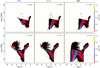Fig. 1.

Phase diagrams at redshift z = 15.0 (upper row) and z = 8.1 (lower row) for the simulations in Table 1 run with UV rates by Puchwein et al. (2019) (P19, left), Faucher-Giguère (2020) (FG20, centre), and Haardt & Madau (1996) (HM, right). The simulation data for temperature, T, and gas overdensity with respect to the gas mean, δ, have been gridded on a base-10 logarithmic scale. The colour coding refers to the total PDF.

Collapsing star forming regions are more sensitive to feedback effects and the implications of different assumptions for feedback parameters might be relevant for the thermodynamical evolution of cosmic gas, independently of the adopted UV prescriptions. As indicative examples, in Fig. 2 we show phase diagrams at redshift z = 6.1 for the runs with SN efficiencies of 0.01–1 and wind velocity of 350 or 700 km s⁻¹ in the HM case. A low SN efficiency of 0.01 (left panel, HM-0.01) is incapable of removing dense material from the star forming regions (at Log₁₀δ ≳ 1), where gas retains temperatures of 10⁴–10⁵ K without cooling further (red/blue branch). A higher efficiency of 1 (central panel, HM-1) removes more gas, as is clear from the probability distribution of the star forming branch (red region at Log₁₀δ ∼ 1–2.5). Such material circulates through the IGM and CGM again and becomes available for further cooling and fragmentation. The 0.1 case with the same winds (not plotted) features an intermediate behaviour. The results displayed in both the left and central panels have a wind velocity of 350 km s⁻¹. Stronger winds with velocities of for example 700 km s⁻¹ (right panel with SN efficiency of 0.1, HM-w700) impact gas removal from star forming sites. In the case shown, dense material is ejected to outer regions more efficiently and abundantly populates the thin IGM at Log₁₀δ ≲ −1 and T ≳ 10⁵ K. Besides the role of wind velocity, other wind parameters, such as the wind delay time before re-coupling to hydrodynamics (e.g., 0.1 t_H adopted in HM-wf, instead of the reference 0.025 t_H adopted in Fig. 2), are expected to have less vital effects. The picture at different redshifts is qualitatively similar, as it is when assuming a Chabrier IMF (HM-Chabrier and HM-1-Chabrier), instead of a standard Salpeter IMF. Alternative UV rates for these models (e.g., P19, P19-1, P19-Chabrier, P19-1-Chabrier) show analogous behaviours, except for the mentioned (temporal) differences. These preliminary considerations highlight the main impact of different assumptions on the UV background and feedback effects, specifically on the thin cosmic medium. The implications for cold dense media (privileged sites hosting neutral and molecular gas) are analyzed in Sect. 3.2.

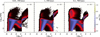Fig. 2.

Phase diagrams at redshift z = 6.1 in scenarios with HM background and, from left to right, a SN efficiency (wind velocity) of: 0.01 (350 km s⁻¹), 1 (350 km s⁻¹), and 0.1 (700 km s⁻¹). These are the runs HM-0.01, HM-1, and HM-w700, respectively.

3.2. Density parameters

In this section, we focus on the evolution of mass density parameters for neutral gas, Ω_neutral, and molecular H₂ gas, Ω_H₂, as extracted from simulation outputs at different times, and compare them to state-of-the-art observational data (Sect. 2.1) in Fig. 3. Theoretical trends refer to runs with the reference implementation including time-dependent non-equilibrium abundance computations, a high-density threshold of 10 cm⁻³ for stochastic star formation, stellar evolution, metal spreading, and H₂ self shielding. We distinguish between simulations accounting for HI self shielding, (HM-HISSmed, P19-HISSmed and FG20-HISSmed denoted by thick lines) and analogous unshielded results (HM, P19 and FG20 denoted by thin lines).

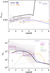Fig. 3.

Upper panel: redshift evolution of Ω_neutral compared to inferred values from HI observations with 1σ error bars (grey points) and corresponding fit (from darker to lighter shades) at 1, 2, and 3σ confidence levels (see Péroux & Howk 2020). The simulations considered are: HM-HISSmed (thick black solid lines), P19-HISSmed (thick blue dashed lines), and FG20-HISSmed (thick orange dot-dot-dot-dashed lines), and all include HI self shielding. As a comparison, corresponding unshielded runs with the same UV backgrounds (HM, P19 and FG20) are displayed by thin lines of the same colour and style. Lower panel: corresponding evolution of Ω_H₂ compared to the observational constraints listed in Table A.1 (PH20 1, 2, and 3σ confidence levels, shades; ALMACAL-CO, light grey; VLASPEC, magenta; PHIBBS-2, purple; COLDz, yellow; ASPECS, green; UKIDSS-UDS, cyan; ALMACAL-abs and Hershel PEP upper and lower limits, dark grey).

In the top panel, we focus on Ω_neutral. We can see that theoretical results increase smoothly with redshift at z ≃ 2–5, in broad agreement with observational data. UV radiation impacts our results after the onset of the UV background and leaves the signal from earlier epochs unaffected (as visible for all the UV models e.g., in Appendix G). In both HI shielded and unshielded HM scenarios, the cold mass surviving at z ≲ 6 after photoionisation is turned on is only 5% of the original cold mass, corresponding to Ω_neutral ∼ 10⁻³. As HI shielding preserves HI mass, the resulting Ω_neutral at z ≃ 2–3 is larger by a factor of up to 2 with respect to the unshielded case. Although both curves are broadly consistent with the available data at z ≲ 5, the unshielded run seems to predict a steeper evolution of cold gas. The shielded HM scenario is slightly above the 1σ error bars of observational data points. In the P19 and FG20 cases the UV model is turned on earlier, resulting in a larger effect of the associated feedback and flatter curves compared to those obtained with an HM background. In these cases, the predictions are slightly below 1σ observational determinations for the unshielded runs, while the corresponding shielded cases are roughly consistent with observational lower limits. The addition of further physical processes, as we see in the following, does not strongly affect Ω_neutral, whose values remain robustly close to the ones displayed in the figure and within the error bars of available data. We note that the displayed fitting expression by Péroux & Howk (2020), namely Ω_neutral ∝ (1 + z)^0.57, is similar to other independent formulations finding Ω_neutral ∝ (1 + z)^0.60 (Crighton et al. 2015) or Ω_neutral ∝ (1 + z)^0.64 (Rao et al. 2017). Thus, uncertainties on the numerical fit do not affect our conclusions.

In the bottom panel of Fig. 3 we explore the outcome for Ω_H₂ compared to the observational constraints (listed in Table A.1) by Hamanowicz et al. (2021) (ALMACAL-CO), Riechers et al. (2020a) (VLASPEC), Lenkić et al. (2020) (PHIBBS-2) Riechers et al. (2020b) (COLDz), Decarli et al. (2020) (ASPECS), and Garratt et al. (2021) (UKIDSS-UDS). For ALMACAL-CO, maximum and minimum values of preliminary estimates at z < 2 are shown. Darker to lighter shades correspond to 1, 2, and 3σ confidence levels by Péroux & Howk (2020). ALMACAL-abs upper limit in the z ≃ 0–2 range is taken by Klitsch et al. (2019) while Herschel PEP most probable lower limit at z ≃ 2–3 is by Berta et al. (2013).

H₂ mass forms in cold high-density regions with rates depending on gas temperature and ionisation state. Therefore, as opposed to Ω_neutral, predicted values for Ω_H₂ are very sensitive to the underlying chemical and physical modelling. We neatly see that HI shielding effects in the HM-HISSmed, P19-HISSmed, and FG20-HISSmed runs are responsible for largely increasing the amount of H₂ with respect to the corresponding unshielded HM, P19, and FG20 results. Indeed, the Ω_H₂ parameter is enhanced by ∼1 dex, while the HI mass increases by only a factor of up to 2. This reveals the highly non-linear nature of the involved chemical processes, as changes of a factor of a few in HI cause much larger variations in H₂. Clearly, the unshielded HM, P19, and FG20 models produce excessive H₂ dissociation and are not consistent with the data (the related Ω_H₂ values fall down to ≲2 × 10⁻⁶ at z ≲ 3, far from observational limits by almost to two orders of magnitude). However, despite the inclusion of HI shielding, the P19 and FG20 scenarios feature an Ω_H₂ evolution that flattens at z ≃ 4–7, hardly reaching Ω_H₂ ∼ 10⁻⁴. This is a result of the earlier onset of the UV background and more powerful rates associated to these two models at such epochs. Conversely, the HI-shielded HM model produces values closer to the observed ones by employing only the essential H₂ formation channels, which are able to enhance the H₂ mass density parameter at z ≃ 4–6 in the presence of a milder UV background. Indeed, the evolution of the H₂ density parameter is affected by the evolution of the photoionisation and photoheating rates adopted in the simulations. The P19 rates evolve smoothly from high redshift until z ≃ 6, where they get enhanced by more than three orders of magnitude, while the FG20 rates at z ≃ 8 go from zero to levels comparable to those of the P19 model. Although newly available free charges induce H₂ formation, on longer timescales the overall effect is H₂ disruption, in shielded as well as unshielded cases. The decline observed in Ω_H₂ at lower redshift is linked to the stronger effect of both UV radiation and star formation, which destroy molecules through photoheating and stellar feedback. The latter is increasingly effective at later times (see e.g., lower-z trends for un-shielded models), while the former depends on the details of the UV background at different z. For an earlier and/or stronger UV background (e.g., P19 and FG20) H₂ suppression is more significant, albeit modulated by gas self shielding.

By looking at Ω_H₂ data in light of our findings, one might think that the large dispersion in the observations at low redshifts (e.g., Klitsch et al. 2019; Decarli et al. 2019, 2020; Riechers et al. 2020b; Garratt et al. 2021) could be related to targeted objects found in conditions that are heterogeneous in terms of gas shielding, heating, ionisation, or photodissociating radiation (hence, the need for large statistical samples). In practice, the right combination of UV model and HI self shielding is needed to match both HI and H₂ data. A UV background turning on at z ≳ 8 seems to induce excessive feedback and predict too little cold gas. This suggests that either UV rates at those times should be lower than those adopted here or high-z gas self shielding should be stronger.

Typically, stochastic conversion of gas into stars is responsible for removing very dense gas parcels from collapsing material. Nevertheless, Ω_neutral and Ω_H₂ parameters might be affected if gas-to-stars conversion involves particles that are still at relatively low density (below ∼1 particle cm⁻³). In this case, the abundance of HI and H₂ cannot grow significantly during their cooling process. To make sure that gas evolution through the cooling branch is followed properly and the amount of HI and H₂ formed is realistic, we have always used a density threshold of 10 cm⁻³, as time-dependent non-equilibrium runaway cooling usually takes place in gas with densities > 0.1 cm⁻³ and temperatures ∼10²−10⁴ K. However, besides the density threshold, gas-to-star conversion is often assumed to depend on gas density, ρ, and a typical star formation timescale, t_sf (see Sect. 2.2.6). This means that the particle SFR is ∝ρ/t_sf. As H₂ molecules are the main drivers of star formation (and not simply the entire gas reservoir) and because we are able to follow their non-equilibrium chemical abundance precisely, in the following we employ the local H₂ density, ρ_H₂, as derived by our non-equilibrium calculations to estimate the particle SFR ∝ρ_H₂/t_sf and related feedback effects (non-equilibrium H₂-based star formation). In Fig. 4 we compare the resulting Ω_neutral and Ω_H₂ parameters for such a scenario (HM-HISSmed-H2 run) to the reference results (HM-HISSmed run). Although the evolution of Ω_neutral and Ω_H₂ obtained with the H₂-based approach is similar to the reference one, it seems to be a better fit to observations of both gas components. With respect to the reference trends, Ω_H₂ values are slightly higher as a consequence of the less effective star formation feedback. Consequently, HI is more easily converted into H₂ and the resulting Ω_neutral values are smaller.

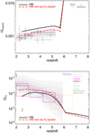Fig. 4.

Upper panel: Ω_neutral evolution for the non-equilibrium H₂-based star formation model (red dashed line, HM-HISSmed-H2) with an HM background and compared to the reference run (solid black line, HM-HISSmed). Lower panel: corresponding Ω_H₂ evolution. Observational determinations are listed in Table A.1 (see also text and Fig. 3).

We additionally investigated the role of individual H₂ formation channels, finding that H⁻ is a fundamental driver at all times, while three-body interactions are less important on large scales. Nevertheless, these latter are useful to reach large H₂ fractions of at least 50% (i.e. ∼67% of the available H mass) even during the epoch of reionisation and explain the 50%−60% values at z ∼ 4–6 recently reported by for example Dessauges-Zavadsky et al. (2020) and Tacconi et al. (2018, 2020) (Appendix F). Including gas-grain processes coupled to the non-equilibrium molecular network and metal spreading leads to a more complete treatment of cold-gas chemistry, without substantially affecting our conclusions. Also, dust grains can enhance H₂ fractions by up to ∼50% by z ≃ 7, in line with observations (for a more detailed discussion see Appendices C and D), but are effective at relatively large metallicities. Heating due to cosmic rays formed in star forming regions is relatively localised and, regardless of the details of the ionisation rates, its impact remains at the 10% level (Appendix E). Feedback due to different SN efficiencies or wind parameterizations impact Ω_neutral and Ω_H₂, inhibiting –more or less efficiently– the amount of cold neutral and molecular gas available. Material in the distant IGM and CGM suffers only mild effects from these events (Appendices H and I).

In summary, we find that to accurately model cold gas and to reproduce the observed atomic and molecular abundances, it is crucial to follow the non-equilibrium chemistry of HI and H₂ self-shielded material down to densities of at least ∼10 cm⁻³ and to resolve the gas runaway cooling. In this way, our results are in better agreement with observations than previous simulation predictions at high z.

3.3. Gas depletion times

Gas depletion times are useful tools with which to investigate the baryon cycle and its relation to cosmic expansion (often parameterized by the Hubble time, t_H). As hot gas is unlikely to collapse, it is natural to focus on cold neutral gas and on molecular H₂-rich gas.

Figure 5 shows the cold-neutral-gas depletion time for different UV models compared to observational data and the Hubble time. For all the UV models, depletion times decrease with decreasing redshift, suggesting that typical cosmic structures can accumulate cold material that will eventually collapse and form stars. This qualitative behaviour is almost universal and little dependent on model details. Quantitatively, results from simulations including HI shielding are more consistent with the data, with values becoming lower than t_H at z ≲ 4. Unshielded models with P19 and FG20 background radiation are only marginally different from observational constraints.

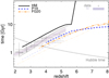Fig. 5.

Redshift evolution of the neutral-gas depletion times in simulations with HM, P19, and FG20 (solid, dashed and dot-dot-dot-dashed lines, respectively) UV backgrounds compared to depletion times with 1σ errors (grey points) derived from Ω_neutral observational data and 1, 2, and 3σ confidence levels (from darker to lighter shades) (see also Fig. 3). Results are for HI shielded (thick) and HI unshielded (thin) scenarios. The Hubble time (grey dotted line) is also shown.

Figure 6 shows the corresponding H₂ depletion times compared to observational data. In this case, besides the Hubble time, we also plot the ‘dynamical’ time, t_dyn, defined as a fraction of 10% of the Hubble time, t_dyn = 0.1 t_H. This expression can be explained with simple dynamical arguments (see Appendix J) and is often quoted in observational studies (Lilly et al. 2013; Tacconi et al. 2020) as indicative of the evolution of a marginally stable rotating disk in which molecular cooling, gas fragmentation, and star formation should take place. In Fig. 6, H₂ global estimates agree well with observational results from alternative galaxy-based approaches that suggest a best-fitting trend of t_depl,H₂(z) = (1.6±0.5)(1+z)−(0.98±0.12) Gyr within 2σ error bars (very close to t_dyn) and data dispersion of almost 1 dex (see Tacconi et al. 2020, who used existing literature data and ALMA archive molecular-mass detections up to z ≃ 5.3). In line with studies of cosmic cold gas showing no explicit dependence on galaxy mass, size, or environment for galaxy-integrated depletion times (Darvish et al. 2018; Tadaki et al. 2019) and notwithstanding the operational costs to determine molecular masses, H₂ depletion times can track cosmic gas evolution if the star formation history is well known (Tacconi et al. 2020). Despite the relatively low scatter at z ≃ 2–4 (between 0.1 and 1 Gyr), lower z determinations have a larger spread. Using available observational data, at z ≃ 0–2 we find t_depl, H₂ comprised between 10 Gyr (ALMACAL-abs upper limits) and 0.01 Gyr (ASPECS and Herschel PEP lower limits). The latest UKIDSS data at z ≃ 2 suggest values of around 0.1–0.3 Gyr. Interestingly, expected H₂ depletion times are always found below the Hubble time and often below the dynamical time. This is a more stringent constraint than the one derived from neutral-gas depletion times and supports the idea that cosmic structures form much beyond redshift z ≃ 6. Thus, future observational efforts in the (sub)mm regimes, leading to observations of larger samples of high-z star forming galaxies, similar to those recently detected at z ≃ 6 (Gruppioni et al. 2020; Talia et al. 2021; Zavala et al. 2021), are required.

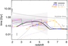Fig. 6.

Redshift evolution of the H₂ depletion time in simulations with HM, P19, and FG20 (solid, dashed and dot-dot-dot-dashed lines, respectively) UV backgrounds. H₂ depletion times within 1σ range (slanted shapes), 1, 2, and 3σ confidence levels (from darker to lighter shades), and maximum and minimum values (grey arrows) are derived from Ω_H₂ observational data and limits in Table A.1 and Fig. 3. The Hubble time (thick grey dotted line) and the dynamical time, t_dyn (thin grey dotted line) are also shown. Results refer to both HI shielded (thick) and HI unshielded (thin) scenarios.

4. Discussion

In the previous sections, we investigate the role of different physical and chemical processes that could affect atomic and molecular cold-gas evolution. We tested three different UV backgrounds (HM, P19, FG20) coupled to non-equilibrium chemistry and find that UV radiation from forming structures has a clear impact on the thermodynamics, composition, and time evolution of cosmic gas. This is generally true for all the UV scenarios examined here, although the implications of each individual model vary remarkably and appear to be extreme for large UV onset redshifts (z ≳ 8).

Inclusion of HI and H₂ self shielding is relevant to address the role of UV photoionisation at high (above 1 particle cm⁻³) and intermediate densities (in the range between ∼10⁻² and 1 particle cm⁻³). HI shielding has an important indirect impact during and after reionisation, because it significantly preserves the amount of HI, which is indispensable for H₂ formation, from UV photoionisation. Thus, self shielding ensures that large enough amounts of HI and H₂ are obtained to consistently match the observations. We remind that H₂ self shielding is effective mainly on dense gas and has little impact on IGM/CGM-like material (e.g., Petkova & Maio 2012), and therefore HI self shielding is found to play a major role in cosmic gas chemistry. The effect of varying H₂ shielding prescriptions, instead, is modest (Appendix B). As an example, the recently updated model by Wolcott-Green et al. (2017) results in excellent agreement with previous works by Draine & Bertoldi (1996) as long as the length scale used to derive the local H₂ column density is approximated by one-quarter of the Jeans length. The effects of alternative choices are small in thin media, but become important in dense sites (e.g., when estimating molecular cooling of collapsing gas or critical fluxes of impinging radiation during the formation of massive black-hole seeds; Luo et al. 2020; Maio et al. 2019). Neglecting HI shielding corrections at high redshift (z > 5) leads to a large degree of H ionisation and H₂ photodissociation, causing underestimation of HI and H₂ cosmological densities and leading to a trend of the atomic and molecular density parameters in tension with data even at z < 5. Furthermore, gas self shielding appears to be crucial for justifying the existence of molecular gas at high redshift, as observed ubiquitously in outflows of massive galaxies at z ≳ 4 with loading factors of the order of unity (Spilker et al. 2020).

Gas-grain processes have been implemented adopting different values for a constant (T_gr = 40, 75 and 120 K) and a z-dependent grain temperature, based either on the CMB scaling or on the dust emissivity index, β (da Cunha et al. 2021). As T_gr evolution is not very sensitive to β, we find that details of its implementation do not have a large impact on the bulk of structure formation and the overall H₂ mass formed; however, they can be relevant locally in metal-rich sites (in agreement with expectations from high-z starburst galaxies; Overzier et al. 2011) and boost molecular fractions above 50% (Appendix C).

Our results show that the origin of H₂ in different epochs is typically linked to free electrons made available during structure formation that boost the H⁻ channel in most cosmic environments. Such a relevant role of the H⁻ channel is in line with conclusions from analytic investigations that stressed the need to reduce the density of H⁻ to suppress star formation in early mini-haloes (Cen 2017), and is also in line with recent semi-analytical ISM studies that highlighted the important role played by H⁻ (Thi et al. 2020). This species is effective in electron-rich, albeit not extremely dense (∼0.1–1 cm⁻³) gas, as is the case for most of the cosmic medium during or after reionisation. Free electrons are captured by H atoms via radiative attachment and increase the amount of H⁻ available for H₂ formation. The $H_{2}^{+}$ ${\rm H}_{2}^{+}$ channel can provide an additional contribution (of up to about one-fifth), but it is typically smaller than that from the H⁻ channel because of the lower collisional rates (Appendix F). Reactions involving H⁻ and $H_{2}^{+}$ ${\rm H}_{2}^{+}$ catalysts that form molecular hydrogen ( $H^{-} + H_{2}^{+} \to H_{2} + H$ $\rm H^- + H_2^+ \rightarrow H_2 + H$ ) are less likely than $H_{2}^{+}$ ${\rm H}_{2}^{+}$ or H⁻ impacts with H and the resulting H₂ enhancement is not substantial, given also their relatively low abundances. Three-body processes can provide some H₂ mass content. Their effects are subdominant for Ω_neutral and Ω_H₂ estimates, but help reach high H₂ fractions of roughly 50% at z ∼ 4–6 in metal-poor sites (i.e. values similar to those reached by H₂ grain catalysis in metal-rich sites).

These processes nicely explain the origin of the large supply of molecular mass within galaxies at z ≳ 2 (Garratt et al. 2021). In fact, large observationally inferred H₂ fractions at early times (Dessauges-Zavadsky et al. 2020) can be explained either via standard H₂ formation channels in metal-poor or pristine gas or via H₂ grain catalysis in metal-rich sites. We warn the reader that, from a purely statistical point of view, large H₂ values, although detected, might not necessarily be typical for the whole galaxy population at those epochs. Indeed, there is a clear observational bias because of which galaxies with large H₂ fractions are easier to observe via their strong CO emission. Previous results from subgrid models for isolated galaxies at z ≃ 2 focusing on H₂ formation on dust grains only (Tomassetti et al. 2015) confirm the leading role of H₂ grain catalysis in enriched environments. The possibility to form H₂ molecules via the two mentioned chemistry paths is also consistent with the lack of observed environmental (metallicity) dependence up to z ∼ 3.5 in the assembly of H₂ mass (e.g., Darvish et al. 2018; Tadaki et al. 2019). This hides the fundamental physical difference between the nearby Universe, where H₂ formation is led by grain catalysis in polluted media (in agreement with results of local molecular clouds; Wakelam et al. 2017), and the distant Universe, where H₂ production is mainly led by the H⁻ channel in shielded low-Z/pristine gas. We warn that, in principle, H₂ production could be enhanced by grain processes at any z, as long as the sites concerned have local metallicities of Z ≳ 0.1 Z_⊙. This conclusion is consistent with detailed ISM analyses by for example Gong et al. (2020) (who consider Z within 0.5–2 Z_⊙) and Hu et al. (2021) (who explore Z within 0.1–3 Z_⊙).

We improve upon previous semi-analytical studies by Jasche et al. (2007) who examined the possible heating due to cosmic rays at early epochs (Appendix E). Our constant cosmic-ray ionisation rate per H atom, ζ = 10⁻¹⁷ s⁻¹, is consistent with traditional values, with the latest determinations by Thi et al. (2020) and with the rate assumed in Narayanan & Krumholz (2017), who correct the suggested ζ ≃ 10⁻¹⁶ s⁻¹ by a factor of 0.1 (Indriolo & McCall 2012). We additionally consider the calculations by Padovani et al. (2018) for a density-dependent ζ and adopt it to assess the implications on star forming gas. We find that typical values for the cosmic-ray ionisation rate induce heating, in addition to the heating from structure formation shocks, and cause a deficit of Ω_H₂ at early times. In the realistic scenario of cosmic-ray heating linked to star forming gas parcels, the effects observed at high z are not very prominent and the resulting Ω_H₂ and Ω_neutral (or Ω_HI) are close to those without cosmic-ray heating. At lower z, the formation of molecular gas is slightly suppressed and Ω_H₂ is slightly smaller than in the reference scenario without cosmic-ray heating. Overall, the effects are of the order of 10%. These results are consistent with the low level (up to a factor of 2) of star formation suppression found in the most recent studies of isolated disk galaxies (Semenov et al. 2021) and hint at the limited role of cosmic-ray heating in high-z structures.

The additional processes mentioned above (metallicity evolution, metal-dependent H₂ grain catalysis, photoelectric effect, cosmic-ray heating, etc.) may have an impact on the local environment, depending on the chemical and thermal state of the hosting gas. H₂ grain catalysis and photoelectric heating can boost Ω_H₂ by up to a factor of 3 at z ≃ 6, still within observational constraints (Riechers et al. 2020b), while large metallicities enhance H₂ grain catalysis up to Ω_H₂ ≃ 2–3 × 10⁻⁴ for Z ∼ Z_⊙. We note that we have scaled the H₂ grain reaction and cooling/heating rates linearly with Z, but dust-to-gas ratios could be steeper in low-Z environments (as in blue compact dwarfs, which can be thought as nearby probes of the physics of distant primeval sources). In such cases, the suggested scaling could be ∝Z^1.5 (Galametz et al. 2011) or even ∝Z² (Herrera-Camus et al. 2012). This would lower the contribution of gas-grain cooling/heating at low Z, imply metallicities closer to solar which would render the H₂ grain catalysis more effective, and indicate a much smaller role of heavy elements at early times. Non-equilibrium results about the cosmic-ray heating rely on the ionisation rate and yield derived from realistic H, He, and H₂ gas mixtures. Although improved with respect to previous works, those quantities are still obtained by neglecting heavy elements, and therefore analyses of the energy transfer in more general conditions are still required. In our study, we varied the ionisation rate by up to one order of magnitude and found small effects for HI and H₂ mass densities in star forming regions at z < 6. Furthermore, we tested the implications of different IMFs and wind assumptions on mass density parameters, but found no significant changes (Appendix I).

The actual role of some physical processes, such as the photoelectric effect, cosmic rays, or dust cycling in galaxies during the epoch of reionisation, is still unclear and more data are needed (Burgarella et al. 2020). Despite these uncertainties, gas self shielding, which preserves HI and H₂ abundances, is likely the principal reason for cool molecular gas to extend further out than dust in observations of star forming galaxies. Indeed, we find that, without self shielding, lower H₂ values are obtained even with the inclusion of H₂ grain catalysis. This is in line with recent interpretations of ALMA observations (Calistro Rivera et al. 2018) and should hold a fortiori at high redshift, when metals and dust grains are expected to be under-abundant. In this respect, observational analyses by Calistro Rivera et al. (2018) support our conclusions.

Earlier cosmological simulations have highlighted the difficulty in reproducing the behaviour of chemical density parameters. In particular, the observed increasing trend of Ω_HI and Ω_neutral has been challenging to model. Numerical efforts by Nagamine et al. (2004) using similar star formation and feedback models to Springel & Hernquist (2003) in a dozen Gadget simulations highlighted the relevant role of wind feedback and obtained Ω_HI results consistent with observations at z = 2–5 with a ‘weak’ wind speed of 242 km s⁻¹. This value is in line with our reference wind speed of 350 km s⁻¹. The consistency in the general trend is encouraging and corroborates the results presented in this manuscript. Nagamine et al. (2004) could not study Ω_H₂ evolution because of a lack of observational data at the time. Davé et al. (2013) proposed a treatment for HI and H₂ gas content based on H ionisation balance to account for HI and on ISM pressure equilibrium to account for H₂. They computed H₂ fractions in star forming particles only. Gas that is not star forming was assumed to have zero molecular content. These approximations were required because the star formation threshold used by the authors was 0.1 cm⁻³ (too low to resolve runaway molecular cooling in dense cold gas) and HI/H₂ self-shielding effects were not included. Gas properties were corrected for HI shielding in post-processing, but they found an HI mass density parameter decreasing with increasing redshift, with Ω_HI < 10⁻³ at z < 5 and Ω_HI ≃ a few 10⁻⁴ at z ≃ 5. These predictions led Davé et al. (2013) to question the ability of equilibrium-based models to capture the fundamental processes shaping the HI and H₂ behaviour, as also noted in Davé et al. (2020). Similarly, low HI mass densities and decreasing Ω_HI redshift evolution have been obtained by other independent groups based on semi-analytical models run on top of N-body simulations (e.g., Spinelli et al. 2020). The deviations of H₂ abundances from equilibrium in cosmic environments highlight the need to follow a time-dependent non-equilibrium approach to obtain reliable molecular fractions (as stressed lately by Hu et al. 2017, 2021, and as done throughout this work). Other popular hydrodynamic simulations (such as Owls or Eagle; Schaye et al. 2015, and references therein) adopt UV rates similar to the ones used here (HM), but employ low-density thresholds for star formation and do not partition hydrogen into its ionised, neutral, and molecular components (as also done in the NIHAO project; Obreja et al. 2019). Post-processing assumptions on how to distribute these species are therefore needed (Blitz & Rosolowsky 2006 or Gnedin & Kravtsov 2011). Post-processing modelling of hydrogen phases for the Eagle simulations (Rahmati et al. 2015) leads to a roughly flat HI curve at z ∼ 2–6, while Illustris-TNG results in a 100 Mpc h⁻¹ side box feature a non-monotonic behaviour attributed to a lack of resolution (Villaescusa-Navarro et al. 2018). As it is usually based on local calibrations, this approach is effective for studying the nearby Universe or enriched systems, but might present issues at higher redshift or in low-metallicity environments, such as the whole epoch of reionisation and the first few cosmological gigayears. In practice, as they are not included in hydrodynamical and chemistry run-time calculations, H₂ molecules cannot play any role in gas cooling. It is probably for this reason that semi-analytical computations by Lagos et al. (2018, and references therein) performed on the outputs of numerical simulations to estimate HI and H₂ fractions with post-processing scaling relations find HI densities which are not fully consistent with observations. Their HI (neutral) mass density parameter decreases from a few 10⁻⁴ (at z ≃ 1) down to 10⁻⁵ (at z ≃ 3.5) and also their values never reach Ω_HI ∼ 10⁻³ (Rhee et al. 2018). Despite that, Lagos et al. (2018) can roughly reproduce Ω_H₂ values at z ≲ 3. The various Illustris simulations (e.g., Springel et al. 2018, and references therein) address HI and H₂ properties via the empirical model of Gnedin & Draine (2014, 2016), but do not implement non-equilibrium atomic and molecular chemistry. When post-processed with semi-analytical models (Somerville et al. 2015), results predict H₂ masses that are too low at z > 1 and cosmic densities (Ω_H₂) in tension with ASPECS data, independently of the adopted H₂ partition recipe, as their simulated gas (for which the star formation density threshold is ∼0.1 cm⁻³) is not dense enough to become molecular (Popping et al. 2019). The smaller Ω_H₂ values found by Popping et al. (2019) might also be linked to the chosen UV background by Faucher-Giguère et al. (2009), which (similarly to Faucher-Giguère 2020, FG20) assumes an earlier onset and hence causes a longer photoheating injection with respect to the HM model. Although this latter is adopted in Lagos et al. (2018), their latest semi-analytical estimates (Lagos et al. 2020) still find ρ_H₂ values systematically below the observational constraints. Other recent studies (such as Gjergo et al. 2018, 2020, Vogelsberger et al. 2019, Graziani et al. 2020, Granato et al. 2021) have incorporated dust mass modelling from gas mass metallicities within three-dimensional numerical simulations, however their implementations are not coupled to non-equilibrium H₂ chemistry. Finally, recent H₂ modelling by Schäbe et al. (2020) that includes H₂ formation via dust grain catalysis only in a 12 Mpc/h side box suggests the existence of undetected molecular amounts at high redshift, as their predicted H₂ mass densities at z ≃ 4−6 were higher than current observational determinations (as in Fig. C.2).

We note that, as in any such work, numerical accuracy is important, but the different star formation schemes and feedback implementations adopted often have a larger impact. Feedback efficiency and star formation timescales modulate the whole evolution of H₂ mass. Changing the shape of the IMF from Salpeter to Chabrier slightly alters star-formation-related quantities (in agreement with e.g., Cassarà et al. 2013), while varying wind velocities (Hassan & Gronke 2021) or SN efficiency has an impact of up to 1 dex when these parameters are varied by a factor of 5–10, independently of other model assumptions (Steinwandel et al. 2020). For HI, the impact is less dramatic and results vary by less than 0.5 dex. Chemistry rates and yields are still affected by factor-of-two uncertainties (for examples, compare H₂ grain catalysis rates in Hollenbach & McKee 1979; Tielens & Hollenbach 1985; Cazaux & Tielens 2004; Tomassetti et al. 2015) and this influences resulting abundance ratios (Maio & Tescari 2015; Ma et al. 2015, 2017b; Valentini et al. 2019a).

From an observational point of view, HI mass densities are relatively well established up to z ≲ 6 with errors below a factor of 2. Moreover, exploiting [C II] emission in high-z enriched environments (as lately done by Heintz et al. 2021) would possibly open the door to observing Ω_neutral at z > 6, where our results predict different scenarios depending on the chosen UV background. On the other hand, estimates of the reservoir of H₂ masses in star forming environments from [C II] or CO observational data are challenging and the conversion factors usually adopted bear uncertainties and biases (Madden et al. 2020; Gong et al. 2020; Breysse et al. 2021). The [C II] 158 micron line is a workhorse for (sub-)mm observations and is resolved on a kiloparsec scale by ALMA (Rybak et al. 2019). As extended [C II] halos are found more and more commonly in high-z galaxies (early star forming sources of 10¹¹–10¹² M_⊙ fit with classical ‘normal’ star forming galaxies; Ginolfi et al. 2019; Hodge & da Cunha 2020) and because [C II] emissions tracing a combination of molecular, ionised, and atomic gas are still very little explored, future assessments of H₂ via [C II] could significantly improve the current picture for Ω_H₂.

Throughout this work we assumed a ΛCDM cosmology. We briefly point out that in some particular cases (such as for warm dark matter, Maio & Viel 2015) the background cosmological model mostly influences the baryonic-structure evolution at higher redshift. This plays a role during the beginning of the onset of star formation, but in the epochs of interest here, baryon evolution tends to dominate and alleviate any discrepancy due either to alternative cosmologies (Maio et al. 2006) and matter non-Gaussianities (Maio & Iannuzzi 2011; Maio 2011; Maio et al. 2012; Maio & Khochfar 2012) or to a different dark-matter nature (Maio & Viel 2015). Finally, the baryon census (Ω_0,b) is crucial for assessing atomic and molecular gas evolution. Alternative estimates of Ω_0,b have been proposed (using e.g., FRBs, Macquart et al. 2020) and, although uncertainties still persist, they are consistent with the cosmic microwave background and Big Bang nucleosynthesis.

5. Conclusions

We quantified the evolution of cold atomic and molecular cosmic gas, from the epoch of reionisation down to z ∼ 2. We performed cosmological N-body hydrodynamic chemistry simulations to model the origin and evolution of cold-gas density parameters and timescales. Our implementation follows time-dependent non-equilibrium atomic and molecular abundance calculations and considers the impact of different UV backgrounds, as well as a number of physical processes that could affect the build-up of H₂ and neutral-gas mass. Star formation in dense HI and H₂ self-shielded regions, stellar feedback, and production of heavy elements from stars with different masses and metallicities are also accounted for. We constrain the effects of the major processes involved in cold-gas evolution and interpret state-of-the-art observations in the (sub-)mm and IR ranges. The present study is among the first of its kind to address cosmic HI and H₂ evolution at these epochs using three-dimensional hydrodynamic simulations and including detailed non-equilibrium chemistry networks. Our findings can be summarised as follows.

The evolution of cold atomic and molecular gas obtained with basic time-dependent non-equilibrium chemical reactions in dense gas is broadly consistent with the latest HI and H₂ observational data once HI and H₂ self shielding from UV radiation is taken into account within the chemical network.
The resulting mass of neutral gas slowly increases with redshift up to Ω_neutral ∼ 2 × 10⁻³ at z ≃ 6, while H₂ features a plateau at Ω_H₂ ∼ 10⁻⁴ at z ≳ 2.
Details of the UV background model adopted (HM, P19 and FG20) have a modest impact on Ω_neutral at z ≲ 6, while they are relevant for Ω_H₂: the onset epoch of the UV background in particular seems to be crucial, suggesting that early (z ≳ 8) onsets could be in tension with H₂ data and could require either lower UV rates or larger self shielding at those times.
Resolving dense shielded gas and adopting a high star formation density threshold is necessary to properly estimate the amount of cold gas and to obtain results in line with HI and H₂ observational data.
Our non-equilibrium H₂-based star formation model leads to results that are in slightly better agreement with available HI and H₂ determinations.
H₂ evolution is globally driven by the H⁻ channel, with a relevant contribution from H₂ grain catalysis at high metallicities and on local scales, while other formation channels are negligible. This explains the observationally inferred lack of environmental dependence in H₂ mass build-up at z ≲ 3.5.
Cosmic-ray heating in star forming regions, quantified in accordance with different models for the cosmic-ray ionisation rate, affects the H₂ abundance at the 10% level globally.
Wind feedback impacts results mostly at lower redshift, while SN explosions affect early star forming regimes, with effects from IMF variations usually remaining small at all times.
Recently detected molecular fractions of ∼50% at z ≃ 4–6 can be explained by essential non-equilibrium H₂ formation channels in metal-poor media or H₂ grain catalysis in metal-rich gas: in this latter case, precise determination of grain temperature has little relevance and is generally subdominant to metallicity effects.
Despite the insurgence of UV radiation, H₂ depletion times reach values that are lower than the Hubble time, and even comparable to the dynamical time, within the first half-gigayear, meaning that cosmic gas is able to collapse already at such early epochs.

The ability to form significant amounts of H₂ and to reach short depletion times during the epoch of reionisation means that further discoveries of molecular-rich star forming galaxies at early times will be possible in the coming years. New data from upcoming international facilities, such as JWST (Gardner & JWST Science Working Group 2009), ELT (Puech et al. 2010), SKA (Koopmans et al. 2015), Roman/WFIRST (Whalen et al. 2013) or ATHENA (Nandra et al. 2013), will be decisive in shedding light on the still unanswered questions about the origin of chemical species in the cosmic gas and the whole baryon cycle.

¹

http://www.vla.nrao.edu/

²

https://www.almaobservatory.org

³

https://www.iram-institute.org/EN/noema-project.php

⁴

http://wsa.roe.ac.uk/UKIRT.html

Acknowledgments

We are grateful to the anonymous referee for his/her careful reading and suggestions that improved the original manuscript. We are thankful to F. Haardt, S. Borgani, L. Tornatore, G. Popping and R. Szakacs for their constructive comments. U.M. is indebted to L. Böss and U. Steinwandel for insightful conversations and to M. Padovani for kindly sharing the full table of his ionisation rate calculations used throughout this work. We thank A. Hamanowicz for sharing with us preliminary ALMACAL-CO results. We also thank the Max Planck Computation and Data Facility (MPCDF) of the Max Planck Society, where simulation runs and analyses have been performed. We acknowledge the NASA Astrophysics Data System and the JSTOR archive for their bibliographic research tools.

References

Abel, T., Anninos, P., Zhang, Y., & Norman, M. L. 1997, New Astron., 2, 181 [NASA ADS] [CrossRef] [Google Scholar]
Abel, T., Bryan, G. L., & Norman, M. L. 2002, Science, 295, 93 [CrossRef] [Google Scholar]
Anninos, P., Zhang, Y., Abel, T., & Norman, M. L. 1997, New Astron., 2, 209 [CrossRef] [Google Scholar]
Bakes, E. L. O., & Tielens, A. G. G. M. 1994, ApJ, 427, 822 [NASA ADS] [CrossRef] [Google Scholar]
Bera, A., Kanekar, N., Chengalur, J. N., & Bagla, J. S. 2019, ApJ, 882, L7 [NASA ADS] [CrossRef] [Google Scholar]
Berta, S., Lutz, D., Nordon, R., et al. 2013, A&A, 555, L8 [NASA ADS] [CrossRef] [EDP Sciences] [Google Scholar]
Binney, J., & Tremaine, S. 2008, Galactic Dynamics: Second Edition (Princeton University Press) [Google Scholar]
Blitz, L., & Rosolowsky, E. 2006, ApJ, 650, 933 [NASA ADS] [CrossRef] [Google Scholar]
Bolatto, A. D., Wolfire, M., & Leroy, A. K. 2013, ARA&A, 51, 207 [CrossRef] [Google Scholar]
Boogaard, L. A., Bouwens, R. J., Riechers, D., et al. 2021, ApJ, 916, 12 [NASA ADS] [CrossRef] [Google Scholar]
Breysse, P. C., Yang, S., Somerville, R. S., et al. 2021, ApJ, submitted, [arXiv:2106.14904] [Google Scholar]
Bromm, V., & Yoshida, N. 2011, ARA&A, 49, 373 [CrossRef] [Google Scholar]
Bron, E., Le Bourlot, J., & Le Petit, F. 2014, A&A, 569, A100 [NASA ADS] [CrossRef] [EDP Sciences] [Google Scholar]
Bruzual, G., & Charlot, S. 2003, MNRAS, 344, 1000 [NASA ADS] [CrossRef] [Google Scholar]
Burgarella, D., Nanni, A., Hirashita, H., et al. 2020, A&A, 637, A32 [NASA ADS] [CrossRef] [EDP Sciences] [Google Scholar]
Calistro Rivera, G., Hodge, J. A., Smail, I., et al. 2018, ApJ, 863, 56 [Google Scholar]
Campisi, M. A., Maio, U., Salvaterra, R., & Ciardi, B. 2011, MNRAS, 416, 2760 [CrossRef] [Google Scholar]
Cassarà, L. P., Piovan, L., Weiss, A., Salaris, M., & Chiosi, C. 2013, MNRAS, 436, 2824 [CrossRef] [Google Scholar]
Cazaux, S., & Tielens, A. G. G. M. 2004, ApJ, 604, 222 [NASA ADS] [CrossRef] [Google Scholar]
Cen, R. 2017, MNRAS, 465, L69 [NASA ADS] [CrossRef] [Google Scholar]
Chabrier, G. 2003, PASP, 115, 763 [Google Scholar]
Chen, Q., Meyer, M., Popping, A., et al. 2021, MNRAS, 508, 2758 [NASA ADS] [CrossRef] [Google Scholar]
Chomiuk, L., & Povich, M. S. 2011, AJ, 142, 197 [Google Scholar]
Christiansen, J. F., Davé, R., Sorini, D., & Anglés-Alcázar, D. 2020, MNRAS, 499, 2617 [NASA ADS] [CrossRef] [Google Scholar]
Crighton, N. H. M., Murphy, M. T., Prochaska, J. X., et al. 2015, MNRAS, 452, 217 [Google Scholar]
da Cunha, E., Groves, B., Walter, F., et al. 2013, ApJ, 766, 13 [Google Scholar]
da Cunha, E., Hodge, J. A., Casey, C. M., et al. 2021, ApJ, 919, 30 [NASA ADS] [CrossRef] [Google Scholar]
Darvish, B., Scoville, N. Z., Martin, C., et al. 2018, ApJ, 860, 111 [NASA ADS] [CrossRef] [Google Scholar]
Davé, R., Katz, N., Oppenheimer, B. D., Kollmeier, J. A., & Weinberg, D. H. 2013, MNRAS, 434, 2645 [CrossRef] [Google Scholar]
Davé, R., Rafieferantsoa, M. H., & Thompson, R. J. 2017, MNRAS, 471, 1671 [CrossRef] [Google Scholar]
Davé, R., Anglés-Alcázar, D., Narayanan, D., et al. 2019, MNRAS, 486, 2827 [Google Scholar]
Davé, R., Crain, R. A., Stevens, A. R. H., et al. 2020, MNRAS, 497, 146 [Google Scholar]
Decarli, R., Walter, F., Gónzalez-López, J., et al. 2019, ApJ, 882, 138 [Google Scholar]
Decarli, R., Aravena, M., Boogaard, L., et al. 2020, ApJ, 902, 110 [Google Scholar]
Delhaize, J., Meyer, M. J., Staveley-Smith, L., & Boyle, B. J. 2013, MNRAS, 433, 1398 [NASA ADS] [CrossRef] [Google Scholar]
Dessauges-Zavadsky, M., Ginolfi, M., Pozzi, F., et al. 2020, A&A, 643, A5 [NASA ADS] [CrossRef] [EDP Sciences] [Google Scholar]
Dickman, R. L., Snell, R. L., & Schloerb, F. P. 1986, ApJ, 309, 326 [NASA ADS] [CrossRef] [Google Scholar]
Dolag, K., Borgani, S., Murante, G., & Springel, V. 2009, MNRAS, 399, 497 [Google Scholar]
Donnari, M., Pillepich, A., Nelson, D., et al. 2019, MNRAS, 485, 4817 [Google Scholar]
Draine, B. T., & Bertoldi, F. 1996, ApJ, 468, 269 [Google Scholar]
Draine, B. T., & Lee, H. M. 1984, ApJ, 285, 89 [NASA ADS] [CrossRef] [Google Scholar]
Draine, B. T., & Li, A. 2007, ApJ, 657, 810 [NASA ADS] [CrossRef] [Google Scholar]
Draine, B. T., & Sutin, B. 1987, ApJ, 320, 803 [NASA ADS] [CrossRef] [Google Scholar]
Duley, W. W. 1996, MNRAS, 279, 591 [NASA ADS] [CrossRef] [Google Scholar]
Dwek, E., & Smith, R. K. 1996, ApJ, 459, 686 [NASA ADS] [CrossRef] [Google Scholar]
Faisst, A. L., Fudamoto, Y., Oesch, P. A., et al. 2020, MNRAS, 498, 4192 [NASA ADS] [CrossRef] [Google Scholar]
Faucher-Giguère, C.-A. 2020, MNRAS, 493, 1614 [Google Scholar]
Faucher-Giguère, C.-A., Lidz, A., Zaldarriaga, M., & Hernquist, L. 2009, ApJ, 703, 1416 [Google Scholar]
Fletcher, T. J., Saintonge, A., Soares, P. S., & Pontzen, A. 2021, MNRAS, 501, 411 [Google Scholar]
Flower, D. R., & Harris, G. J. 2007, MNRAS, 377, 705 [NASA ADS] [CrossRef] [Google Scholar]
Forrey, R. C. 2013, ApJ, 773, L25 [NASA ADS] [CrossRef] [Google Scholar]
Furlong, M., Bower, R. G., Theuns, T., et al. 2015, MNRAS, 450, 4486 [Google Scholar]
Galametz, M., Madden, S. C., Galliano, F., et al. 2011, A&A, 532, A56 [NASA ADS] [CrossRef] [EDP Sciences] [Google Scholar]
Galli, D., & Palla, F. 1998, A&A, 335, 403 [NASA ADS] [Google Scholar]
Gardner, J. P., & JWST Science Working Group 2009, in American Astronomical Society Meeting Abstracts #213, Bull. Am. Astron. Soc., 41, 254 [NASA ADS] [Google Scholar]
Garratt, T. K., Coppin, K. E. K., Geach, J. E., et al. 2021, ApJ, 912, 62 [NASA ADS] [CrossRef] [Google Scholar]
Genel, S., Vogelsberger, M., Springel, V., et al. 2014, MNRAS, 445, 175 [Google Scholar]
Genzel, R., Tacconi, L. J., Combes, F., et al. 2012, ApJ, 746, 69 [Google Scholar]
Ginolfi, M., Schneider, R., Valiante, R., et al. 2019, MNRAS, 483, 1256 [NASA ADS] [CrossRef] [Google Scholar]
Girichidis, P., Offner, S. S. R., Kritsuk, A. G., et al. 2020, Space Sci. Rev., 216, 68 [NASA ADS] [CrossRef] [Google Scholar]
Gjergo, E., Granato, G. L., Murante, G., et al. 2018, MNRAS, 479, 2588 [NASA ADS] [CrossRef] [Google Scholar]
Gjergo, E., Palla, M., Matteucci, F., et al. 2020, MNRAS, 493, 2782 [NASA ADS] [CrossRef] [Google Scholar]
Glassgold, A. E., Galli, D., & Padovani, M. 2012, ApJ, 756, 157 [Google Scholar]
Glover, S. C. O., & Clark, P. C. 2012, MNRAS, 421, 9 [NASA ADS] [Google Scholar]
Glover, S. C. O., & Savin, D. W. 2009, MNRAS, 393, 911 [NASA ADS] [CrossRef] [Google Scholar]
Gnedin, N. Y., & Draine, B. T. 2014, ApJ, 795, 37 [Google Scholar]
Gnedin, N. Y., & Draine, B. T. 2016, ApJ, 830, 54 [NASA ADS] [CrossRef] [Google Scholar]
Gnedin, N. Y., & Kravtsov, A. V. 2011, ApJ, 728, 88 [NASA ADS] [CrossRef] [Google Scholar]
Goldsmith, P. F., & Langer, W. D. 1978, ApJ, 222, 881 [Google Scholar]
Goldsmith, P. F., Liseau, R., Bell, T. A., et al. 2011, ApJ, 737, 96 [Google Scholar]
Gong, M., Ostriker, E. C., Kim, C.-G., & Kim, J.-G. 2020, ApJ, 903, 142 [CrossRef] [Google Scholar]
Granato, G. L., Ragone-Figueroa, C., Taverna, A., et al. 2021, MNRAS, 503, 511 [NASA ADS] [CrossRef] [Google Scholar]
Graziani, L., Schneider, R., Ginolfi, M., et al. 2020, MNRAS, 494, 1071 [NASA ADS] [CrossRef] [Google Scholar]
Gruppioni, C., Béthermin, M., Loiacono, F., et al. 2020, A&A, 643, A8 [NASA ADS] [CrossRef] [EDP Sciences] [Google Scholar]
Gry, C., Boulanger, F., Nehmé, C., et al. 2002, A&A, 391, 675 [NASA ADS] [CrossRef] [EDP Sciences] [Google Scholar]
Haardt, F., & Madau, P. 1996, ApJ, 461, 20 [Google Scholar]
Haardt, F., & Madau, P. 2012, ApJ, 746, 125 [Google Scholar]
Habing, H. J. 1968, Bull. Astron. Inst. Netherlands, 19, 421 [Google Scholar]
Hamanowicz, A., Péroux, C., Zwaan, M., et al. 2021, MNRAS, submitted [Google Scholar]
Hartwig, T., Glover, S. C. O., Klessen, R. S., Latif, M. A., & Volonteri, M. 2015, MNRAS, 452, 1233 [NASA ADS] [CrossRef] [Google Scholar]
Hassan, S., & Gronke, M. 2021, ApJ, 908, 219 [NASA ADS] [CrossRef] [Google Scholar]
Heintz, K. E., Watson, D., Oesch, P. A., Narayanan, D., & Madden, S. C. 2021, ApJ, 922, 147 [NASA ADS] [CrossRef] [Google Scholar]
Herrera-Camus, R., Fisher, D. B., Bolatto, A. D., et al. 2012, ApJ, 752, 112 [NASA ADS] [CrossRef] [Google Scholar]
Hodge, J. A., & da Cunha, E. 2020, R. Soc. Open Sci., 7, 200556 [NASA ADS] [CrossRef] [Google Scholar]
Hollenbach, D., & McKee, C. F. 1979, ApJS, 41, 555 [Google Scholar]
Hollenbach, D., & McKee, C. F. 1989, ApJ, 342, 306 [Google Scholar]
Hollenbach, D. J., & Tielens, A. G. G. M. 1999, Rev. Mod. Phys., 71, 173 [Google Scholar]
Hollenbach, D., Kaufman, M. J., Neufeld, D., Wolfire, M., & Goicoechea, J. R. 2012, ApJ, 754, 105 [Google Scholar]
Hoppmann, L., Staveley-Smith, L., Freudling, W., et al. 2015, MNRAS, 452, 3726 [NASA ADS] [CrossRef] [Google Scholar]
Hu, C.-Y., Naab, T., Glover, S. C. O., Walch, S., & Clark, P. C. 2017, MNRAS, 471, 2151 [NASA ADS] [CrossRef] [Google Scholar]
Hu, W., Hoppmann, L., Staveley-Smith, L., et al. 2019, MNRAS, 489, 1619 [NASA ADS] [CrossRef] [Google Scholar]
Hu, C. Y., Sternberg, A., & van Dishoeck, E. F. 2021, ApJ, 920, 44 [NASA ADS] [CrossRef] [Google Scholar]
Hughes, T. M., Ibar, E., Villanueva, V., et al. 2017, MNRAS, 468, L103 [NASA ADS] [CrossRef] [Google Scholar]
Hunt, L. K., Tortora, C., Ginolfi, M., & Schneider, R. 2020, A&A, 643, A180 [NASA ADS] [CrossRef] [EDP Sciences] [Google Scholar]
Indriolo, N., & McCall, B. J. 2012, ApJ, 745, 91 [NASA ADS] [CrossRef] [Google Scholar]
Indriolo, N., Geballe, T. R., Oka, T., & McCall, B. J. 2007, ApJ, 671, 1736 [NASA ADS] [CrossRef] [Google Scholar]
Jasche, J., Ciardi, B., & Enßlin, T. A. 2007, MNRAS, 380, 417 [NASA ADS] [CrossRef] [Google Scholar]
Jones, M. O., & Bate, M. R. 2018, MNRAS, 480, 2562 [NASA ADS] [CrossRef] [Google Scholar]
Jones, M. G., Haynes, M. P., Giovanelli, R., & Moorman, C. 2018, MNRAS, 477, 2 [Google Scholar]
Jura, M. 1975a, ApJ, 197, 581 [NASA ADS] [CrossRef] [Google Scholar]
Jura, M. 1975b, ApJ, 197, 575 [NASA ADS] [CrossRef] [Google Scholar]
Katz, N. 1992, ApJ, 391, 502 [NASA ADS] [CrossRef] [Google Scholar]
Khusanova, Y., Béthermin, M., Le Fèvre, O., et al. 2021, A&A, 649, A152 [NASA ADS] [CrossRef] [EDP Sciences] [Google Scholar]
Klitsch, A., Zwaan, M. A., Péroux, C., et al. 2019, MNRAS, 482, L65 [NASA ADS] [CrossRef] [Google Scholar]
Komatsu, E., Smith, K. M., Dunkley, J., et al. 2011, ApJS, 192, 18 [Google Scholar]
Koopmans, L., Pritchard, J., Mellema, G., et al. 2015, Advancing Astrophysics with the Square Kilometre Array (AASKA14), 1 [Google Scholar]
Krumholz, M. R., & Gnedin, N. Y. 2011, ApJ, 729, 36 [Google Scholar]
Lagos, C. d. P., Tobar, R. J., & Robotham, A. S. G. 2018, MNRAS, 481, 3573 [CrossRef] [Google Scholar]
Lagos, C. d. P., da Cunha, E., Robotham, A. S. G., et al. 2020, MNRAS, 499, 1948 [CrossRef] [Google Scholar]
Leitherer, C., Schaerer, D., Goldader, J. D., et al. 1999, ApJS, 123, 3 [Google Scholar]
Lenkić, L., Bolatto, A. D., Förster Schreiber, N. M., et al. 2020, AJ, 159, 190 [CrossRef] [Google Scholar]
Lepp, S., & Shull, J. M. 1984, ApJ, 280, 465 [NASA ADS] [CrossRef] [Google Scholar]
Leroy, A. K., Walter, F., Sandstrom, K., et al. 2013, AJ, 146, 19 [Google Scholar]
Licquia, T. C., & Newman, J. A. 2015, ApJ, 806, 96 [NASA ADS] [CrossRef] [Google Scholar]
Lilly, S. J., Carollo, C. M., Pipino, A., Renzini, A., & Peng, Y. 2013, ApJ, 772, 119 [NASA ADS] [CrossRef] [Google Scholar]
Luo, Y., Shlosman, I., Nagamine, K., & Fang, T. 2020, MNRAS, 492, 4917 [NASA ADS] [CrossRef] [Google Scholar]
Ma, Q., Maio, U., Ciardi, B., & Salvaterra, R. 2015, MNRAS, 449, 3006 [NASA ADS] [CrossRef] [Google Scholar]
Ma, Q., Maio, U., Ciardi, B., & Salvaterra, R. 2017a, MNRAS, 466, 1140 [NASA ADS] [CrossRef] [Google Scholar]
Ma, Q., Maio, U., Ciardi, B., & Salvaterra, R. 2017b, MNRAS, 472, 3532 [NASA ADS] [CrossRef] [Google Scholar]
Macquart, J. P., Prochaska, J. X., McQuinn, M., et al. 2020, Nature, 581, 391 [Google Scholar]
Madden, S. C., Poglitsch, A., Geis, N., Stacey, G. J., & Townes, C. H. 1997, ApJ, 483, 200 [NASA ADS] [CrossRef] [Google Scholar]
Madden, S. C., Cormier, D., Hony, S., et al. 2020, A&A, 643, A141 [NASA ADS] [CrossRef] [EDP Sciences] [Google Scholar]
Maio, U. 2011, CQG, 28, 225015 [NASA ADS] [CrossRef] [Google Scholar]
Maio, U. 2021, ArXiv e-prints [arXiv:2111.01804] [Google Scholar]
Maio, U., & Iannuzzi, F. 2011, MNRAS, 415, 3021 [NASA ADS] [CrossRef] [Google Scholar]
Maio, U., & Khochfar, S. 2012, MNRAS, 421, 1113 [NASA ADS] [CrossRef] [Google Scholar]
Maio, U., & Tescari, E. 2015, MNRAS, 453, 3798 [Google Scholar]
Maio, U., & Viel, M. 2015, MNRAS, 446, 2760 [NASA ADS] [CrossRef] [Google Scholar]
Maio, U., Dolag, K., Meneghetti, M., et al. 2006, MNRAS, 373, 869 [NASA ADS] [CrossRef] [Google Scholar]
Maio, U., Dolag, K., Ciardi, B., & Tornatore, L. 2007, MNRAS, 379, 963 [NASA ADS] [CrossRef] [Google Scholar]
Maio, U., Ciardi, B., Yoshida, N., Dolag, K., & Tornatore, L. 2009, A&A, 503, 25 [NASA ADS] [CrossRef] [EDP Sciences] [Google Scholar]
Maio, U., Ciardi, B., Dolag, K., Tornatore, L., & Khochfar, S. 2010, MNRAS, 407, 1003 [CrossRef] [Google Scholar]
Maio, U., Khochfar, S., Johnson, J. L., & Ciardi, B. 2011a, MNRAS, 414, 1145 [NASA ADS] [CrossRef] [Google Scholar]
Maio, U., Koopmans, L. V. E., & Ciardi, B. 2011b, MNRAS, 412, L40 [NASA ADS] [CrossRef] [Google Scholar]
Maio, U., Salvaterra, R., Moscardini, L., & Ciardi, B. 2012, MNRAS, 426, 2078 [NASA ADS] [CrossRef] [Google Scholar]
Maio, U., Petkova, M., De Lucia, G., & Borgani, S. 2016, MNRAS, 460, 3733 [NASA ADS] [CrossRef] [Google Scholar]
Maio, U., Borgani, S., Ciardi, B., & Petkova, M. 2019, PASA, 36, e020 [CrossRef] [Google Scholar]
Maloney, P., & Black, J. H. 1988, ApJ, 325, 389 [NASA ADS] [CrossRef] [Google Scholar]
Mancini, M., Schneider, R., Graziani, L., et al. 2015, MNRAS, 451, L70 [CrossRef] [Google Scholar]
Mancini, M., Schneider, R., Graziani, L., et al. 2016, MNRAS, 462, 3130 [NASA ADS] [CrossRef] [Google Scholar]
Muratov, A. L., Gnedin, O. Y., Gnedin, N. Y., & Zemp, M. 2013, ApJ, 772, 106 [NASA ADS] [CrossRef] [Google Scholar]
Nagamine, K., Springel, V., & Hernquist, L. 2004, MNRAS, 348, 421 [NASA ADS] [CrossRef] [Google Scholar]
Nandra, K., Barret, D., Barcons, X., et al. 2013, ArXiv e-prints [arXiv:1306.2307] [Google Scholar]
Narayanan, D., & Krumholz, M. R. 2017, MNRAS, 467, 50 [NASA ADS] [CrossRef] [Google Scholar]
Neufeld, D. A., & Wolfire, M. G. 2017, ApJ, 845, 163 [Google Scholar]
Noterdaeme, P., Petitjean, P., Ledoux, C., & Srianand, R. 2009, A&A, 505, 1087 [NASA ADS] [CrossRef] [EDP Sciences] [Google Scholar]
Noterdaeme, P., Petitjean, P., Carithers, W. C., et al. 2012, A&A, 547, L1 [NASA ADS] [CrossRef] [EDP Sciences] [Google Scholar]
Obreja, A., Macciò, A. V., Moster, B., et al. 2019, MNRAS, 490, 1518 [CrossRef] [Google Scholar]
Omukai, K., Tsuribe, T., Schneider, R., & Ferrara, A. 2005, ApJ, 626, 627 [NASA ADS] [CrossRef] [Google Scholar]
Opal, C. B., Peterson, W. K., & Beatty, E. C. 1971, J. Chem. Phys., 55, 4100 [CrossRef] [Google Scholar]
Orel, A. E. 1987, J. Chem. Phys., 87, 314 [NASA ADS] [CrossRef] [Google Scholar]
O’Shea, B. W., & Norman, M. L. 2008, ApJ, 673, 14 [CrossRef] [Google Scholar]
Overzier, R. A., Heckman, T. M., Wang, J., et al. 2011, ApJ, 726, L7 [NASA ADS] [CrossRef] [Google Scholar]
Padovani, P., & Matteucci, F. 1993, ApJ, 416, 26 [Google Scholar]
Padovani, M., Galli, D., Ivlev, A. V., Caselli, P., & Ferrara, A. 2018, A&A, 619, A144 [NASA ADS] [CrossRef] [EDP Sciences] [Google Scholar]
Pak, S., Jaffe, D. T., van Dishoeck, E. F., Johansson, L. E. B., & Booth, R. S. 1998, ApJ, 498, 735 [NASA ADS] [CrossRef] [Google Scholar]
Palla, F., Salpeter, E. E., & Stahler, S. W. 1983, ApJ, 271, 632 [NASA ADS] [CrossRef] [Google Scholar]
Pallottini, A., Ferrara, A., Bovino, S., et al. 2017, MNRAS, 471, 4128 [NASA ADS] [CrossRef] [Google Scholar]
Peebles, P. J. E., & Dicke, R. H. 1968, ApJ, 154, 891 [NASA ADS] [CrossRef] [Google Scholar]
Péroux, C., & Howk, J. C. 2020, ARA&A, 58, 363 [CrossRef] [Google Scholar]
Petkova, M., & Maio, U. 2012, MNRAS, 422, 3067 [NASA ADS] [CrossRef] [Google Scholar]
Petkova, M., & Springel, V. 2011, MNRAS, 415, 3731 [NASA ADS] [CrossRef] [Google Scholar]
Planck Collaboration VI. 2020, A&A, 641, A6 [NASA ADS] [CrossRef] [EDP Sciences] [Google Scholar]
Ploeckinger, S., & Schaye, J. 2020, MNRAS, 497, 4857 [CrossRef] [Google Scholar]
Popping, G., Pillepich, A., Somerville, R. S., et al. 2019, ApJ, 882, 137 [NASA ADS] [CrossRef] [Google Scholar]
Puchwein, E., Haardt, F., Haehnelt, M. G., & Madau, P. 2019, MNRAS, 485, 47 [NASA ADS] [CrossRef] [Google Scholar]
Puech, M., Rosati, P., Toft, S., et al. 2010, MNRAS, 402, 903 [NASA ADS] [CrossRef] [Google Scholar]
Rahmati, A., Pawlik, A. H., Raičević, M., & Schaye, J. 2013, MNRAS, 430, 2427 [NASA ADS] [CrossRef] [Google Scholar]
Rahmati, A., Schaye, J., Bower, R. G., et al. 2015, MNRAS, 452, 2034 [CrossRef] [Google Scholar]
Rao, S. M., Turnshek, D. A., Sardane, G. M., & Monier, E. M. 2017, MNRAS, 471, 3428 [Google Scholar]
Rhee, J., Zwaan, M. A., Briggs, F. H., et al. 2013, MNRAS, 435, 2693 [NASA ADS] [CrossRef] [Google Scholar]
Rhee, J., Lah, P., Chengalur, J. N., Briggs, F. H., & Colless, M. 2016, MNRAS, 460, 2675 [NASA ADS] [CrossRef] [Google Scholar]
Rhee, J., Lah, P., Briggs, F. H., et al. 2018, MNRAS, 473, 1879 [NASA ADS] [CrossRef] [Google Scholar]
Riechers, D. A., Boogaard, L. A., Decarli, R., et al. 2020a, ApJ, 896, L21 [NASA ADS] [CrossRef] [Google Scholar]
Riechers, D. A., Hodge, J. A., Pavesi, R., et al. 2020b, ApJ, 895, 81 [Google Scholar]
Rodighiero, G., Enia, A., Delvecchio, I., et al. 2019, ApJ, 877, L38 [NASA ADS] [CrossRef] [Google Scholar]
Röllig, M., Ossenkopf, V., Jeyakumar, S., Stutzki, J., & Sternberg, A. 2006, A&A, 451, 917 [Google Scholar]
Rybak, M., Calistro Rivera, G., Hodge, J. A., et al. 2019, ApJ, 876, 112 [Google Scholar]
Salpeter, E. E. 1955, ApJ, 121, 161 [Google Scholar]
Sánchez, S. F., García-Benito, R., Zibetti, S., et al. 2016, A&A, 594, A36 [Google Scholar]
Saslaw, W. C., & Zipoy, D. 1967, Nature, 216, 976 [NASA ADS] [CrossRef] [Google Scholar]
Schäbe, A., Romano-Díaz, E., Porciani, C., Ludlow, A. D., & Tomassetti, M. 2020, MNRAS, 497, 5008 [CrossRef] [Google Scholar]
Schaye, J., Crain, R. A., Bower, R. G., et al. 2015, MNRAS, 446, 521 [Google Scholar]
Scoville, N. Z., & Solomon, P. M. 1975, ApJ, 199, L105 [NASA ADS] [CrossRef] [Google Scholar]
Semenov, V. A., Kravtsov, A. V., & Caprioli, D. 2021, ApJ, 910, 126 [NASA ADS] [CrossRef] [Google Scholar]
Shaw, G., Ferland, G. J., Henney, W. J., et al. 2009, ApJ, 701, 677 [NASA ADS] [CrossRef] [Google Scholar]
Shull, J. M., Danforth, C. W., & Anderson, K. L. 2021, ApJ, 911, 55 [NASA ADS] [CrossRef] [Google Scholar]
Sillero, E., Tissera, P. B., Lambas, D. G., et al. 2021, MNRAS, 504, 2325 [NASA ADS] [CrossRef] [Google Scholar]
Skinner, D., & Wise, J. H. 2020, MNRAS, 492, 4386 [NASA ADS] [CrossRef] [Google Scholar]
Somerville, R. S., Popping, G., & Trager, S. C. 2015, MNRAS, 453, 4337 [Google Scholar]
Spilker, J. S., Phadke, K. A., Aravena, M., et al. 2020, ApJ, 905, 85 [Google Scholar]
Spinelli, M., Zoldan, A., De Lucia, G., Xie, L., & Viel, M. 2020, MNRAS, 493, 5434 [NASA ADS] [CrossRef] [Google Scholar]
Spitzer, L. J., & Scott, E. H. 1969, ApJ, 158, 161 [NASA ADS] [CrossRef] [Google Scholar]
Springel, V. 2005, MNRAS, 364, 1105 [Google Scholar]
Springel, V., & Hernquist, L. 2003, MNRAS, 339, 289 [Google Scholar]
Springel, V., Pakmor, R., Pillepich, A., et al. 2018, MNRAS, 475, 676 [Google Scholar]
Stahler, S. W., & Palla, F. 2004, The Formation of Stars (Weinheim: Wiley-VCH) [CrossRef] [Google Scholar]
Steinwandel, U. P., Moster, B. P., Naab, T., Hu, C.-Y., & Walch, S. 2020, MNRAS, 495, 1035 [NASA ADS] [CrossRef] [Google Scholar]
Sternberg, A., Le Petit, F., Roueff, E., & Le Bourlot, J. 2014, ApJ, 790, 10 [CrossRef] [Google Scholar]
Tacconi, L. J., Neri, R., Genzel, R., et al. 2013, ApJ, 768, 74 [NASA ADS] [CrossRef] [Google Scholar]
Tacconi, L. J., Genzel, R., Saintonge, A., et al. 2018, ApJ, 853, 179 [Google Scholar]
Tacconi, L. J., Genzel, R., & Sternberg, A. 2020, ARA&A, 58, 157 [NASA ADS] [CrossRef] [Google Scholar]
Tadaki, K.-I., Kodama, T., Hayashi, M., et al. 2019, PASJ, 71, 40 [NASA ADS] [CrossRef] [Google Scholar]
Talia, M., Cimatti, A., Giulietti, M., et al. 2021, ApJ, 909, 23 [NASA ADS] [CrossRef] [Google Scholar]
Tescari, E., Katsianis, A., Wyithe, J. S. B., et al. 2014, MNRAS, 438, 3490 [NASA ADS] [CrossRef] [Google Scholar]
Thi, W. F., Hocuk, S., Kamp, I., et al. 2020, A&A, 634, A42 [NASA ADS] [CrossRef] [EDP Sciences] [Google Scholar]
Thielemann, F.-K., Argast, D., Brachwitz, F., et al. 2003, Nucl. Phys. A, 718, 139 [NASA ADS] [CrossRef] [Google Scholar]
Tielens, A. G. G. M., & Hollenbach, D. 1985, ApJ, 291, 722 [Google Scholar]
Tomassetti, M., Porciani, C., Romano-Díaz, E., & Ludlow, A. D. 2015, MNRAS, 446, 3330 [Google Scholar]
Tornatore, L., Borgani, S., Dolag, K., & Matteucci, F. 2007, MNRAS, 382, 1050 [Google Scholar]
Tornatore, L., Borgani, S., Viel, M., & Springel, V. 2010, MNRAS, 402, 1911 [NASA ADS] [CrossRef] [Google Scholar]
Valentini, M., Chiappini, C., Bossini, D., et al. 2019a, A&A, 627, A173 [NASA ADS] [CrossRef] [EDP Sciences] [Google Scholar]
Valentini, M., Borgani, S., Bressan, A., et al. 2019b, MNRAS, 485, 1384 [NASA ADS] [CrossRef] [Google Scholar]
van den Hoek, L. B., & Groenewegen, M. A. T. 1997, A&AS, 123, 305 [NASA ADS] [CrossRef] [EDP Sciences] [Google Scholar]
Vazdekis, A., Sánchez-Blázquez, P., Falcón-Barroso, J., et al. 2010, MNRAS, 404, 1639 [NASA ADS] [Google Scholar]
Villaescusa-Navarro, F., Genel, S., Castorina, E., et al. 2018, ApJ, 866, 135 [NASA ADS] [CrossRef] [Google Scholar]
Vogelsberger, M., McKinnon, R., O’Neil, S., et al. 2019, MNRAS, 487, 4870 [NASA ADS] [CrossRef] [Google Scholar]
Wakelam, V., Bron, E., Cazaux, S., et al. 2017, Mol. Astrophys., 9, 1 [Google Scholar]
Walter, F., Carilli, C., Neeleman, M., et al. 2020, ApJ, 902, 111 [Google Scholar]
Weingartner, J. C., & Draine, B. T. 2001, ApJS, 134, 263 [CrossRef] [Google Scholar]
Whalen, D. J., Fryer, C. L., Holz, D. E., et al. 2013, ApJ, 762, L6 [NASA ADS] [CrossRef] [Google Scholar]
Wise, J. H., Turk, M. J., Norman, M. L., & Abel, T. 2012a, ApJ, 745, 50 [NASA ADS] [CrossRef] [Google Scholar]
Wise, J. H., Abel, T., Turk, M. J., Norman, M. L., & Smith, B. D. 2012b, MNRAS, 427, 311 [NASA ADS] [CrossRef] [Google Scholar]
Wolcott-Green, J., Haiman, Z., & Bryan, G. L. 2017, MNRAS, 469, 3329 [NASA ADS] [Google Scholar]
Wolfire, M. G., Hollenbach, D., & McKee, C. F. 2010, ApJ, 716, 1191 [Google Scholar]
Wolz, L., Pourtsidou, A., Masui, K. W., et al. 2021, MNRAS, in press, [arXiv:2102.04946] [Google Scholar]
Woosley, S. E., & Weaver, T. A. 1995, ApJS, 101, 181 [Google Scholar]
Woosley, S. E., Heger, A., & Weaver, T. A. 2002, Rev. Mod. Phys., 74, 1015 [NASA ADS] [CrossRef] [Google Scholar]
Yoshida, N., Abel, T., Hernquist, L., & Sugiyama, N. 2003, ApJ, 592, 645 [CrossRef] [Google Scholar]
Zafar, T., Popping, A., & Péroux, C. 2013, A&A, 556, A140 [NASA ADS] [CrossRef] [EDP Sciences] [Google Scholar]
Zanella, A., Daddi, E., Magdis, G., et al. 2018, MNRAS, 481, 1976 [Google Scholar]
Zavala, J. A., Casey, C. M., Manning, S. M., et al. 2021, ApJ, 909, 165 [CrossRef] [Google Scholar]

Appendix A: Data samples

Data samples for H₂ mass density values, ρ_H₂ (and corresponding Ω_H₂), are summarised in Table A.1, where redshift range, H₂ measurements, and publication references are quoted. Many of them are present in Péroux & Howk (2020).

Table A.1.

Observational determinations of molecular (H₂) gas considered in this work.

Appendix B: HI and H₂ self shielding

We write the HI self shielding, f_shield, HI, as a function of H number density, n_H, as:

$\begin{matrix} f_{shield, HI} = 0.985 {[1 + {(\frac{n_{H}}{n_{0}})}^{1.9}]}^{- 2} + 0.015 {(1 + \frac{n_{H}}{n_{0}})}^{- 0.72}, \end{matrix}$ $\begin{aligned} f_{\rm shield, HI} = 0.985 \left[ 1 + \left( \frac{n_{\rm H}}{n_0} \right)^{1.9} \right]^{-2} + 0.015 \left( 1 + \frac{n_{\rm H}}{n_0} \right)^{-0.72}, \end{aligned}$ (B.1)

where n₀ = 0.006 cm⁻³ is a parameter. Asymptotically f_shield, HI converges to 1 for n_H ≪ n₀ and to 0 for n_H ≫ n₀. Besides eq. B.1, we checked that the alternative use of the tables by Rahmati et al. (2013) does not change our findings substantially, although truncation at z = 5 causes an unstable behaviour in abundance calculations around that particular redshift.

For H₂ shielding, we refer to Draine & Bertoldi (1996) (their eq. 36 in most cases and their eq. 37 in selected runs). Alternative formulations for H₂ shielding, such as the revisitations by Sternberg et al. (2014) or Wolcott-Green et al. (2017) of the expressions of Draine & Bertoldi (1996) , have a similar impact on the Ω_H₂ mass density parameter. A detailed comparison of different H₂ shielding models is also done in Luo et al. (2020). Maximum deviations from the reference run, reached locally at different epochs, can be estimated by looking at the maximum H₂ mass fractions recorded at different z. These are more sensitive than Ω_H₂ and are plotted in Fig. B.1 for simulations including H⁻, $H_{2}^{+}$ ${\rm H}_{2}^{+}$ and three-body formation channels, with H₂ self-shielding parameterizations by Draine & Bertoldi (1996) and the more recent Wolcott-Green et al. (2017) one. Although we observe differences of up to an order of magnitude at selected redshifts, overall the maximum H₂ mass fraction reached is not substantially affected by the prescription used to model the H₂ self shielding.

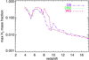Fig. B.1.

Redshift evolution of the maximum H₂ abundance reached in simulations with different H₂ self-shielding formulations: eq. 36 (violet dot-dot-dot-dashed line; HM-HISSmed-3b in Table 1) and eq. 37 (green dotted line; HM-HISSmed-3b-DB2) in Draine & Bertoldi (1996) and the formulation by Wolcott-Green et al. (2017) (magenta dashed line; HM-HISSmed-3b-WG).

Appendix C: H₂ grain catalysis

The rate of H₂ formation due to dust grain catalysis at gas temperature T and grain temperature T_gr is:

$\begin{matrix} k_{H_{2}, gr} = 3.5 \times 10^{- 17} S_{H} \sqrt{\frac{T}{100 K}} {cm}^{3} / s, \end{matrix}$ $\begin{aligned} k_{\rm H_2, gr} = 3.5\times 10^{-17} \, S_{\rm H} \sqrt{ \frac{T}{100\ \mathrm{K}}} \, \mathrm{cm^3/s}, \end{aligned}$ (C.1)

where the sticking coefficient S_H is given by (Hollenbach & McKee 1979; Cazaux & Tielens 2004):

$\begin{matrix} \frac{1}{S_{H}} = 1 + 0.4 \sqrt{\frac{T + T_{gr}}{100 K}} + 0.2 (\frac{T}{100 K}) + 0.08 {(\frac{T}{100 K})}^{2} . \end{matrix}$ $\begin{aligned} \frac{1}{S_{\rm H}} = 1 + 0.4 \sqrt{ \frac{T + T_{\rm gr}}{100\ \mathrm{K}} } + 0.2 \left(\frac{T}{100\ \mathrm{K}}\right) + 0.08 \left(\frac{T}{100\ \mathrm{K}} \right)^2. \end{aligned}$ (C.2)

In the absence of precise determinations at different epochs and Z, k_H₂, gr is linearly scaled by Z, via k_H₂,gr → k_H₂,gr × Z/Z_⊙.

The normalisation of eq. C.1 is similar to the one in Thi et al. (2020) and Sternberg et al. (2014), while Omukai et al. (2005) divide eq. C.1 by 1 + exp[750(1/75 − 1/T_gr)], which suppresses catalysis by a factor ≥2 at grain temperatures T_gr ≥ 75 K. The energy density transfer rate, Λ_gr, is computed accordingly. In the canonical form, calibrated in the near Universe,

$\begin{matrix} Λ_{gr} ≃ 3 \times 10^{- 33} \sqrt{T} (T - T_{gr}) n_{H}^{2} erg / s / {cm}^{3} . \end{matrix}$ $\begin{aligned} \Lambda _{\rm gr} \simeq 3 \times 10^{-33}\sqrt{T}\left( T-T_{\rm gr} \right) \,n_{\rm H}^2 \, \mathrm {erg}/\mathrm {s}/\mathrm {cm}^3. \end{aligned}$ (C.3)

Also in this case there are alternative formulations, as e.g. in Omukai et al. 2005, where the expression is multiplied by the dimensionless factor 1−0.8exp(−75 K/T). Similarly to the H₂ formation rate, the energy density transfer rate is scaled by Z, Λ_gr → Λ_gr ×Z/Z_⊙. We ran simulations by employing both eqs. C.1-C.3 and corrections by Omukai et al. (2005), finding differences of at most a few per cent for the H₂ fractions and median relative variations of the order of 10⁻⁴ for Ω_H₂ values. For HI and neutral gas differences are even smaller.

In Fig. C.1 we explore the effect of T_gr by showing the evolution of the H₂ abundance obtained in simulations with the reference no-catalysis implementation, together with runs including dust grain catalysis with T_gr = 40, 75, and 120 K, as well as a z-dependent T_gr(z) following either the CMB, T_gr(z)=T_0, CMB(1 + z) with T_0,CMB ≃ 2.7 K, or the dust emissivity model with β = 2 (da Cunha et al. 2021). We note that here three-body interactions for H₂ production (considered e.g. in Fig. B.1 and F.1) are switched off. We see that grain catalysis is responsible for increasing maximum H₂ fractions at z ≃ 4-8 up to ∼50% (corresponding to roughly 67% of H mass). This holds independently from the exact value of T_gr, or whether it evolves with redshift. Ω_neutral and Ω_H₂ are unaffected by the exact choices of constant T_gr and are weakly affected from different scaling relations — e.g. T_CMB vs. T_β — for T_gr(z) evolution.

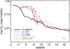Fig. C.1.

Redshift evolution of the maximum H₂ fractions reached in simulations without (solid black line; HM-HISSmed reference run) and with H₂ dust grain catalysis for T_gr= 75 K (purple short-dashed line; HM-HISS-cat-75-Zevol), 40 K (magenta dot-dot-dot-dashed line; HM-HISS-cat-40-Zevol), 120 K (blue dotted line; HM-HISS-cat-120-Zevol), T_gr(z)=T_CMB(z) (green dot-dashed line; HM-HISS-cat-Tcmb-Zevol) and T_gr(z)=T_β(z) with dust emissivity index β = 2 (red long dashed line; HM-HISS-cat-Tbeta-Zevol) are also considered. All the runs include metal spreading from stellar evolution, as indicated in the bottom right corner by Z(t).

In Fig. C.2 we explore the effects of metallicity on H₂ grain catalysis at T_gr = 75 K. Indeed, such H₂ formation process is efficient mostly in cold collapsing gas after metal pollution has started. In addition to the reference simulation, we show results obtained from test runs in which we assume H₂ grain catalysis at fixed Z = Z_⊙ and Z = 0.01 Z_⊙. The largest effects are expected at z ≳ 5, where metallicities have a remarkable impact on Ω_H₂. Typical metallicities in the no-catalysis case are close to zero at z ∼ 20 and reach values around 0.01 Z_⊙ at z ∼ 10, but they have no direct effects on H₂, because grain catalysis is not active. In the law-Z case (Z = 0.01 Z_⊙), we see the formation of an Ω_H₂ ∼ 2 × 10⁻⁶ floor at high redshift that converges at z < 6 to the reference trend. The formation of such a floor is due to additional H₂ formed via grain catalysis in early enriched gas. The increasingly dominant role of UV radiation at z ≲ 6 provides free electrons that enhance H₂ formation in shielded and/or in recombining gas. This is consistent with a leading role played by the H⁻ channel, which becomes more important than law-Z gas-grain processes at the end of reionisation. The extreme Z = Z_⊙ case predicts Ω_H₂ ∼ 1-3 × 10⁻⁴ during most of the cosmological evolution. These values are higher than those expected in the reference run, but one should keep in mind that they are probably unrealistic, as it is unlikely that most of the cosmic gas is polluted at solar metallicity by the first gigayear. In any case, it is a nice confirmation that, at high Z, grain catalysis seems to be the mostly relevant process for Ω_H₂. The effects of UV background onset around z ≃ 6 (with the additional contributions from the H⁻ channel) causes modest adjustments to the otherwise smooth Ω_H₂ evolution. The results obtained with a constant Z highlight how assuming a fixed metallicity floor at early times could drive to misleading conclusions for H₂ estimates (off by orders of magnitude) in the first few billion years.

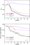Fig. C.2.

Ω_H₂ evolution (upper panel) and maximum H₂ mass fractions (lower panel) reached in the no-catalysis simulation (black solid lines; HM-HISSmed) are compared to runs including H₂ grain catalysis at T_gr = 75 K. Gas Z is either forced to constant values of Z = Z_⊙ (blue dot-dot-dot-dashed lines; HM-HISS-cat-75-Zsun) and 0.01 Z_⊙ (orange dashed lines; HM-HISS-cat-75-0.01Zsun), or consistently computed from temporal evolution of SN II, AGB, and SN Ia metal spreading and cooling from both resonant and fine-structure lines (magenta dot-dashed lines; HM-HISS-cat-75-Zt). Photoelectric heating on dust grains is tested, as well (green dotted lines; HM-HISSmed-cat-75-pe).

Maximum H₂ abundances are clearly boosted at any redshift in the (extreme) case with constant Z = Z_⊙. In the case with a Z = 0.01 Z_⊙ floor, instead, H₂ fractions are quite close to the results expected for the reference (no-catalysis) run at z ≳ 10, but, consistently with Fig. C.1, they show an enhancement at z ≃ 4-8 when H₂ mass fractions reach ∼50% (i.e. 67% with respect to H mass). At z ≳ 8, H₂ fractions are similar in both cases, but corresponding Ω_H₂ values (upper panel) differ as a consequence of the adopted Z floor that enhances H₂ production by a tiny amount in all the gas parcels. The cumulative result tends to an increase of Ω_H₂ by a factor of a few at z ≳ 12. Results from the run including H₂ grain catalysis at T_gr = 75 K and time-dependent metallicity, Z = Z(t), derived from consistent metal evolution and cooling from both resonant and fine-structure lines show a slightly larger Ω_H₂ than the no-catalysis one (due to the generally increasing global metallicities) and an intermediate behaviour of the maximum H₂ fractions (resulting from early local Z values typically comprised within ∼10⁻²-1 Z_⊙; e.g. Maio et al. 2010). Ω_neutral is little affected.

Appendix D: Photoelectric heating

The photoelectric effect in the interstellar medium is caused by the absorption of UV radiation (usually produced by star formation events) from dust grains, which then re-emit electrons and heat up the surrounding medium. Therefore, the power density of photoelectric heating, Γ_pe, is a function of the UV field, parameterized through the dimensionless Habing (1968) parameter G₀ ≃ 1.7, gas temperature, T, and electron number fraction, n_e (Draine & Sutin 1987; Bakes & Tielens 1994; Weingartner & Draine 2001). The efficiency of the process, ε, depends on $G_{0} \sqrt{T} / n_{e}$ $G_0 \sqrt{T} / n_{\mathrm{e}}$ which includes the effects of radiation, recombination rate, and electron number density:

$\begin{matrix} ε (ψ) = \frac{0.0487}{1 + 0.004 ψ^{0.73}} + \frac{0.0365 {(T / 10^{4} K)}^{0.7}}{1 + 0.0002 ψ}, \end{matrix}$ $\begin{aligned} \varepsilon (\psi ) = \frac{0.0487}{1 + 0.004\,\psi ^{0.73} } + \frac{ 0.0365 ( T/10^4\,\mathrm K)^{0.7} }{1 + 0.0002\,\psi } ,\end{aligned}$ (D.1)

where $ψ = G_{0} \sqrt{T} / n_{e}$ $\psi = G_0 \sqrt{T} / n_e$ in units of K^1/2 cm³. The corresponding power density is

$\begin{matrix} Γ_{pe} = C_{pe} ε (ψ) G_{0} n_{H}, \end{matrix}$ $\begin{aligned} \Gamma _{\rm pe} = C_{\rm pe} \ \varepsilon (\psi )\ G_0\ n_{\rm H}, \end{aligned}$ (D.2)

where C_pe ≃ 10⁻²⁴ erg/s is a normalisation factor estimated in the nearby Universe and n_H is the H number density. Because of its dependencies, a quantitative assessment of photoelectric heating needs to be done for all the variety of conditions in which the cosmic gas could possibly be found. Qualitatively, since ε depends inversely on ψ for any fixed G₀, gas at high (low) temperatures experiences limited (relevant) photoelectric heating. Similarly, for a given thermal state, high (low) UV fluxes lead to enhancement (quenching) of Γ_pe. Due to a lack of information about photoelectric heating in the distant Universe, G₀ is either kept constant or scaled by the SFR i.e. G₀ → G₀ × SFR/SFR_⊙, where SFR_⊙ is the Milky Way value. We tried both approaches without finding large differences. As we coupled photoelectric heating with the chemistry network in a flexible way, alternative prescriptions could be tested easily.

To understand the role of this process during cosmological structure formation, in Fig. C.2 we over-plot results for a run including both H₂ grain catalysis with Z given by the actual temporal metallicity evolution and photoelectric heating (dotted lines). The net effect on H₂ mass fractions and mass density parameters results from the trade-off between H₂ enhancement (due to dust grain catalysis) and H₂ dissociation (due to the additional heating mechanism), as clear from the trends in the figure. Compared to the reference no-catalysis case, the final H₂ mass fractions reached (lower panel) in the presence of both photoelectric heating and H₂ grain catalysis is not larger than a factor of 2. Albeit modest, this enhancement involves regions that are increasingly enriched during cosmic time and progressively more abundantly distributed in cosmic space. The cumulative effect on Ω_H₂ (upper panel) is marginal at z ≳ 10, but becomes visible later on, causing a steeper trend at z ≃ 6-10. At z ≲ 6, newly available free electrons from re-ionisation lead, also in this case, to H₂ formation.

Compared to the case including metal cooling (dot-dashed lines), the photoelectric effect is subdominant. Ω_neutral is little changed.

Appendix E: Fitting formula for cosmic-ray ionisation rate ζ(N) and H₂ mass build-up

A fit for the Padovani et al. (2018) tabulated ℒ model as a function of the gas column density, N, in units of 10¹⁹ cm⁻², N₁₉ = N/(10¹⁹ cm⁻²), is given by:

$\begin{matrix} ζ (N_{19}) = a N_{19}^{α} {(1 + \frac{N_{19}}{b})}^{β} e^{- {(N_{19} / c)}^{γ}}, \end{matrix}$ $\begin{aligned} \zeta (N_{19}) = a \,\, N_{19}^\alpha \,\, \left( 1+ \frac{N_{19}}{b} \right)^\beta \mathrm{e}^{-(N_{19}/c)^\gamma }, \end{aligned}$ (E.1)

where a = 3.7221566 × 10⁻¹⁶ s⁻¹ is the normalisation required to reproduce the Padovani et al. (2018)ζ value at N = 10¹⁹ cm⁻² (N₁₉ = 1). The other dimensionless parameters are: b = 10², c = 2 × 10⁶, α = −1/2, β = 1/3 and γ = 7/10. So, ζ scales as $N_{19}^{- 1 / 2}$ $N_{19}^{-1/2}$ at N₁₉ ≪ b, evolves roughly as $N_{19}^{- 1 / 6}$ $N_{19}^{-1/6}$ in the range b ≪ N₁₉ ≪ c and decays exponentially at N₁₉ ≫ c. Since this formulation is tested on the nearby Universe, it is customal to scale ζ, which is mostly related to SN events, by the gas SFR with respect to the local one, SFR_⊙, i.e. ζ → ζ × SFR/SFR_⊙ (e.g. Narayanan & Krumholz 2017).

We test the effects of cosmic-ray heating on the H₂ evolution by employing a constant homogeneous ionisation rate of ζ ≃ 10⁻¹⁷ s⁻¹ per H atom, as well as the density-dependent one by Padovani et al. (2018) (eq. E.1). We also run this latter case considering cosmic-ray heating only in star forming regions, in which ζ is scaled by the gas SFR. The resulting evolution of the H₂ mass density is displayed in Fig. E.1, where we additionally show the case with no cosmic-ray heating for comparison. In general, the presence of a cosmic-ray heating floor (as in e.g. the ζ constant case, dotted line) enhances the amounts of free electrons already at early times and this can increase the formation of H₂ at z ≳ 12 by a factor of ∼4. Nevertheless, the additional heating from ongoing structure formation at later times leads to negative feedback effects and causes the subsequent decrease of Ω_H₂. As a result, at z < 12 the system reaches a new equilibrium for H₂ creation and destruction processes and Ω_H₂ stays below the reference no-heating trend by almost a factor of 3 at z ≃ 4. The Padovani et al. (2018) rate is stronger by up to more than 1 dex, and therefore, if applied to all particles, creates a heating floor that easily ionises gas and dissociates H₂ even at higher redshifts. At lower redshift the resulting Ω_H₂ behaviour converges to the constant ζ case. Applying such a model to star forming particles only smooths the extreme behaviour at early times and allows us to recover an evolution of Ω_H₂ at low z that is similar to, although slightly smaller than (by less than a factor of 2), the reference one at z < 6. We conclude that cosmic-ray heating may affect H₂ abundances during the epoch of reionisation and afterwards. The impact is up to a few tens of per cent for the more realistic SFR-linked case. We note that cosmic-ray heating in the early Universe typically inhibits the $H_{2}^{+}$ ${\rm H}_{2}^{+}$ channel. Indeed, through interactions with cosmic-ray protons, $H_{2}^{+}$ ${\rm H}_{2}^{+}$ is quickly converted into $H_{3}^{+}$ ${\rm H}_{3}^{+}$ . This latter is an unimportant coolant that contributes no more than a few per cent of the total cooling (Glover & Savin 2009) and at large densities, where the gas tends to become fully neutral, suffers from H⁺ removal, dissociative recombination, and H-impact dissociation. Maximum molecular fractions reached are consistent with those derived in the previous cases as well as the density parameters of HI/neutral gas for the SFR-linked case. In the other cases, Ω_neutral values at z < 5 converge to slightly lower values than the reference ones. While the homogeneous presence of cosmic-ray heating is an idealized test case, we can consider as a fiducial model the one including cosmic-ray heating in star forming regions according to the Padovani et al. (2018) description.

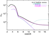Fig. E.1.

Ω_H₂ evolution when cosmic-ray heating included in the reference implementation (black solid line, HM-HISSmed). The case of a constant homogeneous ζ = 10⁻¹⁷ s⁻¹ (turquoise dotted line, HM-HISSmed-cr) is displayed together with two cases in which Padovani et al. (2018)’s ζ is adopted either for all gas parcels (violet dot-dashed line, HM-HISSmed-crP18) or scaled by the local gas SFR (magenta dashed line, HM-HISSmed-crP18sfr).

Appendix F: H₂ formation channels

H₂ formation can be led by different pristine-chemistry processes. To understand which of these is the main driver of Ω_H₂ evolution, we examine the effects of the $H_{2}^{+}$ ${\rm H}_{2}^{+}$ , H⁻ and three-body channels (for the latter we follow Forrey 2013, which improves on previous studies by e.g. Palla et al. 1983, Orel 1987, Abel et al. 2002 and Flower & Harris 2007). In all the runs we include HI shielding (eq. B.1) and H₂ shielding (Draine & Bertoldi 1996). Figure F.1 displays the evolution of Ω_H₂ (top panel) and of the maximum H₂ mass fraction (bottom panel). Three-body interactions dominate H₂ formation in dense, cold regions, where HI atoms are abundant, however they do not impact significantly the global Ω_H₂ values reached by $H_{2}^{+}$ ${\rm H}_{2}^{+}$ and H⁻ channels (upper panel). Compared to the case with only $H_{2}^{+}$ ${\rm H}_{2}^{+}$ and H⁻ channels, three-body processes locally enhanced H₂ formation by a factor of almost 10 at z ≲ 8, raising the H₂ mass fractions to about 50% by the end of reionisation (lower panel). To understand better the relative role played by the H⁻ and $H_{2}^{+}$ ${\rm H}_{2}^{+}$ channels, in Fig. F.1 we show results from simulations including only the $H_{2}^{+}$ ${\rm H}_{2}^{+}$ channel or neither. When no H₂ formation channel is considered, both Ω_H₂ and H₂ fractions remain practically constant at the initial-condition values. Adding the $H_{2}^{+}$ ${\rm H}_{2}^{+}$ formation channel increases both the H₂ density parameter and the H₂ fraction, but resulting values are still well below the required ones. Reliable values are obtained by including, besides the $H_{2}^{+}$ ${\rm H}_{2}^{+}$ , the H⁻ channel, which appears to be crucial for H₂ pristine chemistry. This can be understood in light of the sparsity of high-density regions (this limits the role of three-body processes), the large amount of cosmic gas at moderate densities (above 0.1-1 cm⁻³) with temperatures ≲10⁴ K and the larger reaction rates of the H⁻ channel with respect to the $H_{2}^{+}$ ${\rm H}_{2}^{+}$ .

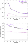Fig. F.1.

Redshift evolution of Ω_H₂ (upper panel) and H₂ (lower) fractions obtained in the reference run (black solid line; HM-HISSmed in Table 1), as well as in simulations including also three-body processes (violet triple-dot-dashed line; HM-HISSmed-3b), only the $H_{2}^{+}$ ${\rm H}_{2}^{+}$ channel (purple dashed line; HM-HISSmed- $H_{2}^{+}$ ${\rm H}_{2}^{+}$ ), and none of the H₂ channels (grey dotted line; HM-HISSmed-none).

Appendix G: Comparison of UV background effects

In Fig. G.1 we quantify the impact of different UV backgrounds on the amount of cold gas, showing the evolution of Ω_neutral and Ω_H₂ for un-shielded HM, P19 and FG20 runs with the basic implementation. For all the UV background scenarios, Ω_neutral is higher than Ω_H₂ at all redshifts. At high z, before the onset of photoheating processes, the HI content is much larger than the one of H₂, reflecting the primordial chemical composition of a mostly neutral cosmic gas with neutral fractions close to the baryon fraction (Ω_0,b ≃ 0.045) and molecular fractions around 10⁻⁶. At later times, Ω_neutral decreases and Ω_H₂ increases with a relative ratio shrinking by a few dex. The displayed trends are sensitive to the onset of the UV background at z ≃ 6, 8.3, 15.1 for HM, FG20 and P19, respectively, when the transition from a neutral to an ionised phase is initiated. Then, Ω_neutral deviates from its initial value ∼0.045, while molecular gas responds to the new thermal conditions. The HM and FG20 scenarios produce similar results at z ≳ 8 (when neither background is turned on), but at lower z the larger FG20 rates are able to ionise gas and dissociate molecules more efficiently than the HM. For example, FG20 HI and HeI rates at z ≃ 6 are ∼10⁻¹² s⁻¹, while HM rates are below 10⁻¹⁵ s⁻¹. At the same z, FG20 HI and HeI heating power is above 10⁻²⁴ erg/s, while the HM ones are below 10⁻²⁶ erg/s. A peculiarity of the P19 model is its strength at early times, which causes H photoionisation by z ≃ 14, when minimal levels of Ω_neutral∼ few 10⁻⁴ and Ω_H₂ ∼ 10⁻⁷ are reached. Later on, with gas cooling re-balancing heating, some HI reforms and H₂ catches up.

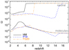Fig. G.1.

Redshift evolution of the neutral and molecular density parameters for the HM (solid black lines), P19 (dashed blue) and FG20 (dot-dot-dot-dashed orange) simulations, respectively.

Appendix H: Impact of SNe

In Fig. H.1, we show Ω_neutral and Ω_H₂ as extracted from simulations including different SN efficiencies with a standard HM background, complementing our previous discussion of Fig. 2. Efficiencies larger than the reference 0.1 value are suited for extremely powerful population-III sources, which would inhibit H₂ and star formation in the first few Gyr. When compared to the reference 0.1 case, values of the molecular-gas density parameters, Ω_H₂, are lower (higher) for SN efficiencies of 0.5-1 (0.01). That is a result of the more (less) efficient molecular-gas removal from star forming regions by stronger (weaker) feedback and the major (minor) destruction of H₂ into HI. Correspondingly, Ω_neutral values increase smoothly until z ≲ 6 at slightly lower (higher) levels when weaker (stronger) feedback is active. Qualitatively, these conclusions hold independently from the UV background (e.g. P19, which is not shown for clarity) and the variations found are comparable to those from other effects, such as cosmic-ray heating in star forming regions.

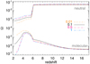Fig. H.1.

Redshift evolution of the neutral and molecular density parameters in models with SN efficiency of 0.1 (black solid line, HM), 0.01 (yellow dot-dashed line, HM-0.01), 0.5 (magenta-red dashed line, HM-0.5) and 1 (azure dot-dot-dot-dashed line, HM-1).

Appendix I: The role of IMF and winds

In Fig. I.1, we compare the effects of different IMFs for various feedback schemes. We consider as reference a simulation with HM background, Salpeter IMF, SN efficiency of 0.1, 350 km/s wind velocity and wind delay time of 0.025 the Hubble time. This simulation is re-run with variations including: a Chabrier IMF, a Chabrier IMF with unitary SN efficiency, a wind velocity of 700 km/s and a longer wind delay time 0.1 the Hubble time. Effects of a Chabrier IMF are small and results tend to follow the evolution of the corresponding runs with a Salpeter IMF. The small effects due to changes of the IMF originate from the small difference in the injected entropy and the SN rates varying only by a factor of 1.4. The model with Chabrier IMF and unitary SN efficiency features some departures from the reference for both Ω_neutral and Ω_H₂, indicating a more relevant role of the feedback scheme. In the case with wind velocity of 700 km/s, the results are very close to those of the reference model. Changing other wind parameters, such as the wind delay time to get re-coupled to hydrodynamic, has no dramatic effect. Similar conclusions hold for different-UV scenarios, too.

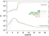Fig. I.1.

Redshift evolution of the neutral and molecular density parameters for the HM background setup, having wind velocity of 350 km/s, wind delay time of 0.025 Hubble time and a Salpeter IMF (black solid lines, HM). Results obtained by increasing, the wind velocity to 700 km/s (pink dotted lines, HM-w700), the wind delay time to 0.1 Hubble time (pink dashed lines, HM-wf) and by adopting a Chabrier IMF (green dot-dashed lines, HM-Chabrier) or a Chabrier IMF with unitary SN efficiency (green dot-dot-dot-dashed lines, HM-1-Chabrier) are shown, too.

Appendix J: Estimates of the dynamical time

A test mass released from rest at distance r from the center of the gravitational potential of a constant density field, ρ, under assumption of spherical symmetry, moves according to the equation of motion of a harmonic oscillator:

$\begin{matrix} \ddot{r} = - \frac{G M (r)}{r^{2}} = - \frac{4 π G ρ}{3} r, \end{matrix}$ $\begin{aligned} \ddot{r} = - \frac{G M(r) }{r^2} = - \frac{ 4 \pi G \rho }{3} r, \end{aligned}$ (J.1)

being G the gravitational constant and M(r) the mass enclosed within r. The angular frequency ω satisfies the relation ω² = 4πGρ/3 and the period is

$\begin{matrix} T = \frac{2 π}{ω} = \sqrt{\frac{3 π}{G ρ}} . \end{matrix}$ $\begin{aligned} T = \frac{ 2 \pi }{ \omega } = \sqrt{ \frac{ 3 \pi }{ G \rho } }. \end{aligned}$ (J.2)

The test mass reaches the center in 1/4 the oscillation period, i.e. in a dynamical time, t_dyn (e.g. Binney & Tremaine 2008):

$\begin{matrix} t_{dyn} \equiv \frac{T}{4} = \sqrt{\frac{3 π}{16 G ρ}} . \end{matrix}$ $\begin{aligned} t_{\rm dyn} \equiv \frac{T}{4} = \sqrt{ \frac{ 3 \pi }{ 16 G \rho } }. \end{aligned}$ (J.3)

If, at any given redshift, ρ ≡ Δ ρ_crit, the critical density is ρ_crit = 3H²/(8πG), and the Hubble time is t_H = 1/H, then

$\begin{matrix} t_{dyn} = \sqrt{\frac{3 π}{16 G Δ ρ_{crit}}} = \frac{π}{\sqrt{2 Δ}} t_{H}, \end{matrix}$ $\begin{aligned} t_{\rm dyn} = \sqrt{ \frac{ 3 \pi }{ 16 G \Delta \rho _{\rm crit}} } = \frac{ \pi }{ \sqrt{2 \Delta } } \ t_{\rm H}, \end{aligned}$ (J.4)

For Δ ≃ 100 up to 2000, t_dyn decreases from t_dyn ≃ 0.2 t_H down to 0.05 t_H. A typical value of Δ ≃ 500 (corresponding to ∼1800 times the mean matter density, or about 10⁴ times the mean baryon density) leads to t_dyn ≃ 0.1 t_H.

All Tables

Table 1.

Inputs to simulation models.

In the text

Table A.1.

Observational determinations of molecular (H₂) gas considered in this work.

In the text

All Figures

Fig. 1.

Phase diagrams at redshift z = 15.0 (upper row) and z = 8.1 (lower row) for the simulations in Table 1 run with UV rates by Puchwein et al. (2019) (P19, left), Faucher-Giguère (2020) (FG20, centre), and Haardt & Madau (1996) (HM, right). The simulation data for temperature, T, and gas overdensity with respect to the gas mean, δ, have been gridded on a base-10 logarithmic scale. The colour coding refers to the total PDF.

In the text

	Fig. 2. Phase diagrams at redshift z = 6.1 in scenarios with HM background and, from left to right, a SN efficiency (wind velocity) of: 0.01 (350 km s⁻¹), 1 (350 km s⁻¹), and 0.1 (700 km s⁻¹). These are the runs HM-0.01, HM-1, and HM-w700, respectively.
In the text

Fig. 3.

Upper panel: redshift evolution of Ω_neutral compared to inferred values from HI observations with 1σ error bars (grey points) and corresponding fit (from darker to lighter shades) at 1, 2, and 3σ confidence levels (see Péroux & Howk 2020). The simulations considered are: HM-HISSmed (thick black solid lines), P19-HISSmed (thick blue dashed lines), and FG20-HISSmed (thick orange dot-dot-dot-dashed lines), and all include HI self shielding. As a comparison, corresponding unshielded runs with the same UV backgrounds (HM, P19 and FG20) are displayed by thin lines of the same colour and style. Lower panel: corresponding evolution of Ω_H₂ compared to the observational constraints listed in Table A.1 (PH20 1, 2, and 3σ confidence levels, shades; ALMACAL-CO, light grey; VLASPEC, magenta; PHIBBS-2, purple; COLDz, yellow; ASPECS, green; UKIDSS-UDS, cyan; ALMACAL-abs and Hershel PEP upper and lower limits, dark grey).

In the text

	Fig. 4. Upper panel: Ω_neutral evolution for the non-equilibrium H₂-based star formation model (red dashed line, HM-HISSmed-H2) with an HM background and compared to the reference run (solid black line, HM-HISSmed). Lower panel: corresponding Ω_H₂ evolution. Observational determinations are listed in Table A.1 (see also text and Fig. 3).
In the text

Fig. 5.

Redshift evolution of the neutral-gas depletion times in simulations with HM, P19, and FG20 (solid, dashed and dot-dot-dot-dashed lines, respectively) UV backgrounds compared to depletion times with 1σ errors (grey points) derived from Ω_neutral observational data and 1, 2, and 3σ confidence levels (from darker to lighter shades) (see also Fig. 3). Results are for HI shielded (thick) and HI unshielded (thin) scenarios. The Hubble time (grey dotted line) is also shown.

In the text

Fig. 6.

Redshift evolution of the H₂ depletion time in simulations with HM, P19, and FG20 (solid, dashed and dot-dot-dot-dashed lines, respectively) UV backgrounds. H₂ depletion times within 1σ range (slanted shapes), 1, 2, and 3σ confidence levels (from darker to lighter shades), and maximum and minimum values (grey arrows) are derived from Ω_H₂ observational data and limits in Table A.1 and Fig. 3. The Hubble time (thick grey dotted line) and the dynamical time, t_dyn (thin grey dotted line) are also shown. Results refer to both HI shielded (thick) and HI unshielded (thin) scenarios.

In the text

	Fig. B.1. Redshift evolution of the maximum H₂ abundance reached in simulations with different H₂ self-shielding formulations: eq. 36 (violet dot-dot-dot-dashed line; HM-HISSmed-3b in Table 1) and eq. 37 (green dotted line; HM-HISSmed-3b-DB2) in Draine & Bertoldi (1996) and the formulation by Wolcott-Green et al. (2017) (magenta dashed line; HM-HISSmed-3b-WG).
In the text

Fig. C.1.

Redshift evolution of the maximum H₂ fractions reached in simulations without (solid black line; HM-HISSmed reference run) and with H₂ dust grain catalysis for T_gr= 75 K (purple short-dashed line; HM-HISS-cat-75-Zevol), 40 K (magenta dot-dot-dot-dashed line; HM-HISS-cat-40-Zevol), 120 K (blue dotted line; HM-HISS-cat-120-Zevol), T_gr(z)=T_CMB(z) (green dot-dashed line; HM-HISS-cat-Tcmb-Zevol) and T_gr(z)=T_β(z) with dust emissivity index β = 2 (red long dashed line; HM-HISS-cat-Tbeta-Zevol) are also considered. All the runs include metal spreading from stellar evolution, as indicated in the bottom right corner by Z(t).

In the text

Fig. C.2.

Ω_H₂ evolution (upper panel) and maximum H₂ mass fractions (lower panel) reached in the no-catalysis simulation (black solid lines; HM-HISSmed) are compared to runs including H₂ grain catalysis at T_gr = 75 K. Gas Z is either forced to constant values of Z = Z_⊙ (blue dot-dot-dot-dashed lines; HM-HISS-cat-75-Zsun) and 0.01 Z_⊙ (orange dashed lines; HM-HISS-cat-75-0.01Zsun), or consistently computed from temporal evolution of SN II, AGB, and SN Ia metal spreading and cooling from both resonant and fine-structure lines (magenta dot-dashed lines; HM-HISS-cat-75-Zt). Photoelectric heating on dust grains is tested, as well (green dotted lines; HM-HISSmed-cat-75-pe).

In the text

Fig. E.1.

Ω_H₂ evolution when cosmic-ray heating included in the reference implementation (black solid line, HM-HISSmed). The case of a constant homogeneous ζ = 10⁻¹⁷ s⁻¹ (turquoise dotted line, HM-HISSmed-cr) is displayed together with two cases in which Padovani et al. (2018)’s ζ is adopted either for all gas parcels (violet dot-dashed line, HM-HISSmed-crP18) or scaled by the local gas SFR (magenta dashed line, HM-HISSmed-crP18sfr).

In the text

Fig. F.1.

Redshift evolution of Ω_H₂ (upper panel) and H₂ (lower) fractions obtained in the reference run (black solid line; HM-HISSmed in Table 1), as well as in simulations including also three-body processes (violet triple-dot-dashed line; HM-HISSmed-3b), only the $H_{2}^{+}$ ${\rm H}_{2}^{+}$ channel (purple dashed line; HM-HISSmed- $H_{2}^{+}$ ${\rm H}_{2}^{+}$ ), and none of the H₂ channels (grey dotted line; HM-HISSmed-none).

In the text

	Fig. G.1. Redshift evolution of the neutral and molecular density parameters for the HM (solid black lines), P19 (dashed blue) and FG20 (dot-dot-dot-dashed orange) simulations, respectively.
In the text

	Fig. H.1. Redshift evolution of the neutral and molecular density parameters in models with SN efficiency of 0.1 (black solid line, HM), 0.01 (yellow dot-dashed line, HM-0.01), 0.5 (magenta-red dashed line, HM-0.5) and 1 (azure dot-dot-dot-dashed line, HM-1).
In the text

Fig. I.1.

Redshift evolution of the neutral and molecular density parameters for the HM background setup, having wind velocity of 350 km/s, wind delay time of 0.025 Hubble time and a Salpeter IMF (black solid lines, HM). Results obtained by increasing, the wind velocity to 700 km/s (pink dotted lines, HM-w700), the wind delay time to 0.1 Hubble time (pink dashed lines, HM-wf) and by adopting a Chabrier IMF (green dot-dashed lines, HM-Chabrier) or a Chabrier IMF with unitary SN efficiency (green dot-dot-dot-dashed lines, HM-1-Chabrier) are shown, too.

In the text

Current usage metrics show cumulative count of Article Views (full-text article views including HTML views, PDF and ePub downloads, according to the available data) and Abstracts Views on Vision4Press platform.

Data correspond to usage on the plateform after 2015. The current usage metrics is available 48-96 hours after online publication and is updated daily on week days.

Initial download of the metrics may take a while.

[1] Abel, T., Anninos, P., Zhang, Y., & Norman, M. L. 1997, New Astron., 2, 181 [NASA ADS] [CrossRef] [Google Scholar]

[2] Abel, T., Bryan, G. L., & Norman, M. L. 2002, Science, 295, 93 [CrossRef] [Google Scholar]

[3] Anninos, P., Zhang, Y., Abel, T., & Norman, M. L. 1997, New Astron., 2, 209 [CrossRef] [Google Scholar]

[4] Bakes, E. L. O., & Tielens, A. G. G. M. 1994, ApJ, 427, 822 [NASA ADS] [CrossRef] [Google Scholar]

[5] Bera, A., Kanekar, N., Chengalur, J. N., & Bagla, J. S. 2019, ApJ, 882, L7 [NASA ADS] [CrossRef] [Google Scholar]

[6] Berta, S., Lutz, D., Nordon, R., et al. 2013, A&A, 555, L8 [NASA ADS] [CrossRef] [EDP Sciences] [Google Scholar]

[7] Binney, J., & Tremaine, S. 2008, Galactic Dynamics: Second Edition (Princeton University Press) [Google Scholar]

[8] Blitz, L., & Rosolowsky, E. 2006, ApJ, 650, 933 [NASA ADS] [CrossRef] [Google Scholar]

[9] Bolatto, A. D., Wolfire, M., & Leroy, A. K. 2013, ARA&A, 51, 207 [CrossRef] [Google Scholar]

[10] Boogaard, L. A., Bouwens, R. J., Riechers, D., et al. 2021, ApJ, 916, 12 [NASA ADS] [CrossRef] [Google Scholar]

[11] Breysse, P. C., Yang, S., Somerville, R. S., et al. 2021, ApJ, submitted, [arXiv:2106.14904] [Google Scholar]

[12] Bromm, V., & Yoshida, N. 2011, ARA&A, 49, 373 [CrossRef] [Google Scholar]

[13] Bron, E., Le Bourlot, J., & Le Petit, F. 2014, A&A, 569, A100 [NASA ADS] [CrossRef] [EDP Sciences] [Google Scholar]

[14] Bruzual, G., & Charlot, S. 2003, MNRAS, 344, 1000 [NASA ADS] [CrossRef] [Google Scholar]

[15] Burgarella, D., Nanni, A., Hirashita, H., et al. 2020, A&A, 637, A32 [NASA ADS] [CrossRef] [EDP Sciences] [Google Scholar]

[16] Calistro Rivera, G., Hodge, J. A., Smail, I., et al. 2018, ApJ, 863, 56 [Google Scholar]

[17] Campisi, M. A., Maio, U., Salvaterra, R., & Ciardi, B. 2011, MNRAS, 416, 2760 [CrossRef] [Google Scholar]

[18] Cassarà, L. P., Piovan, L., Weiss, A., Salaris, M., & Chiosi, C. 2013, MNRAS, 436, 2824 [CrossRef] [Google Scholar]

[19] Cazaux, S., & Tielens, A. G. G. M. 2004, ApJ, 604, 222 [NASA ADS] [CrossRef] [Google Scholar]

[20] Cen, R. 2017, MNRAS, 465, L69 [NASA ADS] [CrossRef] [Google Scholar]

[21] Chabrier, G. 2003, PASP, 115, 763 [Google Scholar]

[22] Chen, Q., Meyer, M., Popping, A., et al. 2021, MNRAS, 508, 2758 [NASA ADS] [CrossRef] [Google Scholar]

[23] Chomiuk, L., & Povich, M. S. 2011, AJ, 142, 197 [Google Scholar]

[24] Christiansen, J. F., Davé, R., Sorini, D., & Anglés-Alcázar, D. 2020, MNRAS, 499, 2617 [NASA ADS] [CrossRef] [Google Scholar]

[25] Crighton, N. H. M., Murphy, M. T., Prochaska, J. X., et al. 2015, MNRAS, 452, 217 [Google Scholar]

[26] da Cunha, E., Groves, B., Walter, F., et al. 2013, ApJ, 766, 13 [Google Scholar]

[27] da Cunha, E., Hodge, J. A., Casey, C. M., et al. 2021, ApJ, 919, 30 [NASA ADS] [CrossRef] [Google Scholar]

[28] Darvish, B., Scoville, N. Z., Martin, C., et al. 2018, ApJ, 860, 111 [NASA ADS] [CrossRef] [Google Scholar]

[29] Davé, R., Katz, N., Oppenheimer, B. D., Kollmeier, J. A., & Weinberg, D. H. 2013, MNRAS, 434, 2645 [CrossRef] [Google Scholar]

[30] Davé, R., Rafieferantsoa, M. H., & Thompson, R. J. 2017, MNRAS, 471, 1671 [CrossRef] [Google Scholar]

[31] Davé, R., Anglés-Alcázar, D., Narayanan, D., et al. 2019, MNRAS, 486, 2827 [Google Scholar]

[32] Davé, R., Crain, R. A., Stevens, A. R. H., et al. 2020, MNRAS, 497, 146 [Google Scholar]

[33] Decarli, R., Walter, F., Gónzalez-López, J., et al. 2019, ApJ, 882, 138 [Google Scholar]

[34] Decarli, R., Aravena, M., Boogaard, L., et al. 2020, ApJ, 902, 110 [Google Scholar]

[35] Delhaize, J., Meyer, M. J., Staveley-Smith, L., & Boyle, B. J. 2013, MNRAS, 433, 1398 [NASA ADS] [CrossRef] [Google Scholar]

[36] Dessauges-Zavadsky, M., Ginolfi, M., Pozzi, F., et al. 2020, A&A, 643, A5 [NASA ADS] [CrossRef] [EDP Sciences] [Google Scholar]

[37] Dickman, R. L., Snell, R. L., & Schloerb, F. P. 1986, ApJ, 309, 326 [NASA ADS] [CrossRef] [Google Scholar]

[38] Dolag, K., Borgani, S., Murante, G., & Springel, V. 2009, MNRAS, 399, 497 [Google Scholar]

[39] Donnari, M., Pillepich, A., Nelson, D., et al. 2019, MNRAS, 485, 4817 [Google Scholar]

[40] Draine, B. T., & Bertoldi, F. 1996, ApJ, 468, 269 [Google Scholar]

[41] Draine, B. T., & Lee, H. M. 1984, ApJ, 285, 89 [NASA ADS] [CrossRef] [Google Scholar]

[42] Draine, B. T., & Li, A. 2007, ApJ, 657, 810 [NASA ADS] [CrossRef] [Google Scholar]

[43] Draine, B. T., & Sutin, B. 1987, ApJ, 320, 803 [NASA ADS] [CrossRef] [Google Scholar]

[44] Duley, W. W. 1996, MNRAS, 279, 591 [NASA ADS] [CrossRef] [Google Scholar]

[45] Dwek, E., & Smith, R. K. 1996, ApJ, 459, 686 [NASA ADS] [CrossRef] [Google Scholar]

[46] Faisst, A. L., Fudamoto, Y., Oesch, P. A., et al. 2020, MNRAS, 498, 4192 [NASA ADS] [CrossRef] [Google Scholar]

[47] Faucher-Giguère, C.-A. 2020, MNRAS, 493, 1614 [Google Scholar]

[48] Faucher-Giguère, C.-A., Lidz, A., Zaldarriaga, M., & Hernquist, L. 2009, ApJ, 703, 1416 [Google Scholar]

[49] Fletcher, T. J., Saintonge, A., Soares, P. S., & Pontzen, A. 2021, MNRAS, 501, 411 [Google Scholar]

[50] Flower, D. R., & Harris, G. J. 2007, MNRAS, 377, 705 [NASA ADS] [CrossRef] [Google Scholar]

[51] Forrey, R. C. 2013, ApJ, 773, L25 [NASA ADS] [CrossRef] [Google Scholar]

[52] Furlong, M., Bower, R. G., Theuns, T., et al. 2015, MNRAS, 450, 4486 [Google Scholar]

[53] Galametz, M., Madden, S. C., Galliano, F., et al. 2011, A&A, 532, A56 [NASA ADS] [CrossRef] [EDP Sciences] [Google Scholar]

[54] Galli, D., & Palla, F. 1998, A&A, 335, 403 [NASA ADS] [Google Scholar]

[55] Gardner, J. P., & JWST Science Working Group 2009, in American Astronomical Society Meeting Abstracts #213, Bull. Am. Astron. Soc., 41, 254 [NASA ADS] [Google Scholar]

[56] Garratt, T. K., Coppin, K. E. K., Geach, J. E., et al. 2021, ApJ, 912, 62 [NASA ADS] [CrossRef] [Google Scholar]

[57] Genel, S., Vogelsberger, M., Springel, V., et al. 2014, MNRAS, 445, 175 [Google Scholar]

[58] Genzel, R., Tacconi, L. J., Combes, F., et al. 2012, ApJ, 746, 69 [Google Scholar]

[59] Ginolfi, M., Schneider, R., Valiante, R., et al. 2019, MNRAS, 483, 1256 [NASA ADS] [CrossRef] [Google Scholar]

[60] Girichidis, P., Offner, S. S. R., Kritsuk, A. G., et al. 2020, Space Sci. Rev., 216, 68 [NASA ADS] [CrossRef] [Google Scholar]

[61] Gjergo, E., Granato, G. L., Murante, G., et al. 2018, MNRAS, 479, 2588 [NASA ADS] [CrossRef] [Google Scholar]

[62] Gjergo, E., Palla, M., Matteucci, F., et al. 2020, MNRAS, 493, 2782 [NASA ADS] [CrossRef] [Google Scholar]

[63] Glassgold, A. E., Galli, D., & Padovani, M. 2012, ApJ, 756, 157 [Google Scholar]

[64] Glover, S. C. O., & Clark, P. C. 2012, MNRAS, 421, 9 [NASA ADS] [Google Scholar]

[65] Glover, S. C. O., & Savin, D. W. 2009, MNRAS, 393, 911 [NASA ADS] [CrossRef] [Google Scholar]

[66] Gnedin, N. Y., & Draine, B. T. 2014, ApJ, 795, 37 [Google Scholar]

[67] Gnedin, N. Y., & Draine, B. T. 2016, ApJ, 830, 54 [NASA ADS] [CrossRef] [Google Scholar]

[68] Gnedin, N. Y., & Kravtsov, A. V. 2011, ApJ, 728, 88 [NASA ADS] [CrossRef] [Google Scholar]

[69] Goldsmith, P. F., & Langer, W. D. 1978, ApJ, 222, 881 [Google Scholar]

[70] Goldsmith, P. F., Liseau, R., Bell, T. A., et al. 2011, ApJ, 737, 96 [Google Scholar]

[71] Gong, M., Ostriker, E. C., Kim, C.-G., & Kim, J.-G. 2020, ApJ, 903, 142 [CrossRef] [Google Scholar]

[72] Granato, G. L., Ragone-Figueroa, C., Taverna, A., et al. 2021, MNRAS, 503, 511 [NASA ADS] [CrossRef] [Google Scholar]

[73] Graziani, L., Schneider, R., Ginolfi, M., et al. 2020, MNRAS, 494, 1071 [NASA ADS] [CrossRef] [Google Scholar]

[74] Gruppioni, C., Béthermin, M., Loiacono, F., et al. 2020, A&A, 643, A8 [NASA ADS] [CrossRef] [EDP Sciences] [Google Scholar]

[75] Gry, C., Boulanger, F., Nehmé, C., et al. 2002, A&A, 391, 675 [NASA ADS] [CrossRef] [EDP Sciences] [Google Scholar]

[76] Haardt, F., & Madau, P. 1996, ApJ, 461, 20 [Google Scholar]

[77] Haardt, F., & Madau, P. 2012, ApJ, 746, 125 [Google Scholar]

[78] Habing, H. J. 1968, Bull. Astron. Inst. Netherlands, 19, 421 [Google Scholar]

[79] Hamanowicz, A., Péroux, C., Zwaan, M., et al. 2021, MNRAS, submitted [Google Scholar]

[80] Hartwig, T., Glover, S. C. O., Klessen, R. S., Latif, M. A., & Volonteri, M. 2015, MNRAS, 452, 1233 [NASA ADS] [CrossRef] [Google Scholar]

[81] Hassan, S., & Gronke, M. 2021, ApJ, 908, 219 [NASA ADS] [CrossRef] [Google Scholar]

[82] Heintz, K. E., Watson, D., Oesch, P. A., Narayanan, D., & Madden, S. C. 2021, ApJ, 922, 147 [NASA ADS] [CrossRef] [Google Scholar]

[83] Herrera-Camus, R., Fisher, D. B., Bolatto, A. D., et al. 2012, ApJ, 752, 112 [NASA ADS] [CrossRef] [Google Scholar]

[84] Hodge, J. A., & da Cunha, E. 2020, R. Soc. Open Sci., 7, 200556 [NASA ADS] [CrossRef] [Google Scholar]

[85] Hollenbach, D., & McKee, C. F. 1979, ApJS, 41, 555 [Google Scholar]

[86] Hollenbach, D., & McKee, C. F. 1989, ApJ, 342, 306 [Google Scholar]

[87] Hollenbach, D. J., & Tielens, A. G. G. M. 1999, Rev. Mod. Phys., 71, 173 [Google Scholar]

[88] Hollenbach, D., Kaufman, M. J., Neufeld, D., Wolfire, M., & Goicoechea, J. R. 2012, ApJ, 754, 105 [Google Scholar]

[89] Hoppmann, L., Staveley-Smith, L., Freudling, W., et al. 2015, MNRAS, 452, 3726 [NASA ADS] [CrossRef] [Google Scholar]

[90] Hu, C.-Y., Naab, T., Glover, S. C. O., Walch, S., & Clark, P. C. 2017, MNRAS, 471, 2151 [NASA ADS] [CrossRef] [Google Scholar]

[91] Hu, W., Hoppmann, L., Staveley-Smith, L., et al. 2019, MNRAS, 489, 1619 [NASA ADS] [CrossRef] [Google Scholar]

[92] Hu, C. Y., Sternberg, A., & van Dishoeck, E. F. 2021, ApJ, 920, 44 [NASA ADS] [CrossRef] [Google Scholar]

[93] Hughes, T. M., Ibar, E., Villanueva, V., et al. 2017, MNRAS, 468, L103 [NASA ADS] [CrossRef] [Google Scholar]

[94] Hunt, L. K., Tortora, C., Ginolfi, M., & Schneider, R. 2020, A&A, 643, A180 [NASA ADS] [CrossRef] [EDP Sciences] [Google Scholar]

[95] Indriolo, N., & McCall, B. J. 2012, ApJ, 745, 91 [NASA ADS] [CrossRef] [Google Scholar]

[96] Indriolo, N., Geballe, T. R., Oka, T., & McCall, B. J. 2007, ApJ, 671, 1736 [NASA ADS] [CrossRef] [Google Scholar]

[97] Jasche, J., Ciardi, B., & Enßlin, T. A. 2007, MNRAS, 380, 417 [NASA ADS] [CrossRef] [Google Scholar]

[98] Jones, M. O., & Bate, M. R. 2018, MNRAS, 480, 2562 [NASA ADS] [CrossRef] [Google Scholar]

[99] Jones, M. G., Haynes, M. P., Giovanelli, R., & Moorman, C. 2018, MNRAS, 477, 2 [Google Scholar]

[100] Jura, M. 1975a, ApJ, 197, 581 [NASA ADS] [CrossRef] [Google Scholar]

[101] Jura, M. 1975b, ApJ, 197, 575 [NASA ADS] [CrossRef] [Google Scholar]

[102] Katz, N. 1992, ApJ, 391, 502 [NASA ADS] [CrossRef] [Google Scholar]

[103] Khusanova, Y., Béthermin, M., Le Fèvre, O., et al. 2021, A&A, 649, A152 [NASA ADS] [CrossRef] [EDP Sciences] [Google Scholar]

[104] Klitsch, A., Zwaan, M. A., Péroux, C., et al. 2019, MNRAS, 482, L65 [NASA ADS] [CrossRef] [Google Scholar]

[105] Komatsu, E., Smith, K. M., Dunkley, J., et al. 2011, ApJS, 192, 18 [Google Scholar]

[106] Koopmans, L., Pritchard, J., Mellema, G., et al. 2015, Advancing Astrophysics with the Square Kilometre Array (AASKA14), 1 [Google Scholar]

[107] Krumholz, M. R., & Gnedin, N. Y. 2011, ApJ, 729, 36 [Google Scholar]

[108] Lagos, C. d. P., Tobar, R. J., & Robotham, A. S. G. 2018, MNRAS, 481, 3573 [CrossRef] [Google Scholar]

[109] Lagos, C. d. P., da Cunha, E., Robotham, A. S. G., et al. 2020, MNRAS, 499, 1948 [CrossRef] [Google Scholar]

[110] Leitherer, C., Schaerer, D., Goldader, J. D., et al. 1999, ApJS, 123, 3 [Google Scholar]

[111] Lenkić, L., Bolatto, A. D., Förster Schreiber, N. M., et al. 2020, AJ, 159, 190 [CrossRef] [Google Scholar]

[112] Lepp, S., & Shull, J. M. 1984, ApJ, 280, 465 [NASA ADS] [CrossRef] [Google Scholar]

[113] Leroy, A. K., Walter, F., Sandstrom, K., et al. 2013, AJ, 146, 19 [Google Scholar]

[114] Licquia, T. C., & Newman, J. A. 2015, ApJ, 806, 96 [NASA ADS] [CrossRef] [Google Scholar]

[115] Lilly, S. J., Carollo, C. M., Pipino, A., Renzini, A., & Peng, Y. 2013, ApJ, 772, 119 [NASA ADS] [CrossRef] [Google Scholar]

[116] Luo, Y., Shlosman, I., Nagamine, K., & Fang, T. 2020, MNRAS, 492, 4917 [NASA ADS] [CrossRef] [Google Scholar]

[117] Ma, Q., Maio, U., Ciardi, B., & Salvaterra, R. 2015, MNRAS, 449, 3006 [NASA ADS] [CrossRef] [Google Scholar]

[118] Ma, Q., Maio, U., Ciardi, B., & Salvaterra, R. 2017a, MNRAS, 466, 1140 [NASA ADS] [CrossRef] [Google Scholar]

[119] Ma, Q., Maio, U., Ciardi, B., & Salvaterra, R. 2017b, MNRAS, 472, 3532 [NASA ADS] [CrossRef] [Google Scholar]

[120] Macquart, J. P., Prochaska, J. X., McQuinn, M., et al. 2020, Nature, 581, 391 [Google Scholar]

[121] Madden, S. C., Poglitsch, A., Geis, N., Stacey, G. J., & Townes, C. H. 1997, ApJ, 483, 200 [NASA ADS] [CrossRef] [Google Scholar]

[122] Madden, S. C., Cormier, D., Hony, S., et al. 2020, A&A, 643, A141 [NASA ADS] [CrossRef] [EDP Sciences] [Google Scholar]

[123] Maio, U. 2011, CQG, 28, 225015 [NASA ADS] [CrossRef] [Google Scholar]

[124] Maio, U. 2021, ArXiv e-prints [arXiv:2111.01804] [Google Scholar]

[125] Maio, U., & Iannuzzi, F. 2011, MNRAS, 415, 3021 [NASA ADS] [CrossRef] [Google Scholar]

[126] Maio, U., & Khochfar, S. 2012, MNRAS, 421, 1113 [NASA ADS] [CrossRef] [Google Scholar]

[127] Maio, U., & Tescari, E. 2015, MNRAS, 453, 3798 [Google Scholar]

[128] Maio, U., & Viel, M. 2015, MNRAS, 446, 2760 [NASA ADS] [CrossRef] [Google Scholar]

[129] Maio, U., Dolag, K., Meneghetti, M., et al. 2006, MNRAS, 373, 869 [NASA ADS] [CrossRef] [Google Scholar]

[130] Maio, U., Dolag, K., Ciardi, B., & Tornatore, L. 2007, MNRAS, 379, 963 [NASA ADS] [CrossRef] [Google Scholar]

[131] Maio, U., Ciardi, B., Yoshida, N., Dolag, K., & Tornatore, L. 2009, A&A, 503, 25 [NASA ADS] [CrossRef] [EDP Sciences] [Google Scholar]

[132] Maio, U., Ciardi, B., Dolag, K., Tornatore, L., & Khochfar, S. 2010, MNRAS, 407, 1003 [CrossRef] [Google Scholar]

[133] Maio, U., Khochfar, S., Johnson, J. L., & Ciardi, B. 2011a, MNRAS, 414, 1145 [NASA ADS] [CrossRef] [Google Scholar]

[134] Maio, U., Koopmans, L. V. E., & Ciardi, B. 2011b, MNRAS, 412, L40 [NASA ADS] [CrossRef] [Google Scholar]

[135] Maio, U., Salvaterra, R., Moscardini, L., & Ciardi, B. 2012, MNRAS, 426, 2078 [NASA ADS] [CrossRef] [Google Scholar]

[136] Maio, U., Petkova, M., De Lucia, G., & Borgani, S. 2016, MNRAS, 460, 3733 [NASA ADS] [CrossRef] [Google Scholar]

[137] Maio, U., Borgani, S., Ciardi, B., & Petkova, M. 2019, PASA, 36, e020 [CrossRef] [Google Scholar]

[138] Maloney, P., & Black, J. H. 1988, ApJ, 325, 389 [NASA ADS] [CrossRef] [Google Scholar]

[139] Mancini, M., Schneider, R., Graziani, L., et al. 2015, MNRAS, 451, L70 [CrossRef] [Google Scholar]

[140] Mancini, M., Schneider, R., Graziani, L., et al. 2016, MNRAS, 462, 3130 [NASA ADS] [CrossRef] [Google Scholar]

[141] Muratov, A. L., Gnedin, O. Y., Gnedin, N. Y., & Zemp, M. 2013, ApJ, 772, 106 [NASA ADS] [CrossRef] [Google Scholar]

[142] Nagamine, K., Springel, V., & Hernquist, L. 2004, MNRAS, 348, 421 [NASA ADS] [CrossRef] [Google Scholar]

[143] Nandra, K., Barret, D., Barcons, X., et al. 2013, ArXiv e-prints [arXiv:1306.2307] [Google Scholar]

[144] Narayanan, D., & Krumholz, M. R. 2017, MNRAS, 467, 50 [NASA ADS] [CrossRef] [Google Scholar]

[145] Neufeld, D. A., & Wolfire, M. G. 2017, ApJ, 845, 163 [Google Scholar]

[146] Noterdaeme, P., Petitjean, P., Ledoux, C., & Srianand, R. 2009, A&A, 505, 1087 [NASA ADS] [CrossRef] [EDP Sciences] [Google Scholar]

[147] Noterdaeme, P., Petitjean, P., Carithers, W. C., et al. 2012, A&A, 547, L1 [NASA ADS] [CrossRef] [EDP Sciences] [Google Scholar]

[148] Obreja, A., Macciò, A. V., Moster, B., et al. 2019, MNRAS, 490, 1518 [CrossRef] [Google Scholar]

[149] Omukai, K., Tsuribe, T., Schneider, R., & Ferrara, A. 2005, ApJ, 626, 627 [NASA ADS] [CrossRef] [Google Scholar]

[150] Opal, C. B., Peterson, W. K., & Beatty, E. C. 1971, J. Chem. Phys., 55, 4100 [CrossRef] [Google Scholar]

[151] Orel, A. E. 1987, J. Chem. Phys., 87, 314 [NASA ADS] [CrossRef] [Google Scholar]

[152] O’Shea, B. W., & Norman, M. L. 2008, ApJ, 673, 14 [CrossRef] [Google Scholar]

[153] Overzier, R. A., Heckman, T. M., Wang, J., et al. 2011, ApJ, 726, L7 [NASA ADS] [CrossRef] [Google Scholar]

[154] Padovani, P., & Matteucci, F. 1993, ApJ, 416, 26 [Google Scholar]

[155] Padovani, M., Galli, D., Ivlev, A. V., Caselli, P., & Ferrara, A. 2018, A&A, 619, A144 [NASA ADS] [CrossRef] [EDP Sciences] [Google Scholar]

[156] Pak, S., Jaffe, D. T., van Dishoeck, E. F., Johansson, L. E. B., & Booth, R. S. 1998, ApJ, 498, 735 [NASA ADS] [CrossRef] [Google Scholar]

[157] Palla, F., Salpeter, E. E., & Stahler, S. W. 1983, ApJ, 271, 632 [NASA ADS] [CrossRef] [Google Scholar]

[158] Pallottini, A., Ferrara, A., Bovino, S., et al. 2017, MNRAS, 471, 4128 [NASA ADS] [CrossRef] [Google Scholar]

[159] Peebles, P. J. E., & Dicke, R. H. 1968, ApJ, 154, 891 [NASA ADS] [CrossRef] [Google Scholar]

[160] Péroux, C., & Howk, J. C. 2020, ARA&A, 58, 363 [CrossRef] [Google Scholar]

[161] Petkova, M., & Maio, U. 2012, MNRAS, 422, 3067 [NASA ADS] [CrossRef] [Google Scholar]

[162] Petkova, M., & Springel, V. 2011, MNRAS, 415, 3731 [NASA ADS] [CrossRef] [Google Scholar]

[163] Planck Collaboration VI. 2020, A&A, 641, A6 [NASA ADS] [CrossRef] [EDP Sciences] [Google Scholar]

[164] Ploeckinger, S., & Schaye, J. 2020, MNRAS, 497, 4857 [CrossRef] [Google Scholar]

[165] Popping, G., Pillepich, A., Somerville, R. S., et al. 2019, ApJ, 882, 137 [NASA ADS] [CrossRef] [Google Scholar]

[166] Puchwein, E., Haardt, F., Haehnelt, M. G., & Madau, P. 2019, MNRAS, 485, 47 [NASA ADS] [CrossRef] [Google Scholar]

[167] Puech, M., Rosati, P., Toft, S., et al. 2010, MNRAS, 402, 903 [NASA ADS] [CrossRef] [Google Scholar]

[168] Rahmati, A., Pawlik, A. H., Raičević, M., & Schaye, J. 2013, MNRAS, 430, 2427 [NASA ADS] [CrossRef] [Google Scholar]

[169] Rahmati, A., Schaye, J., Bower, R. G., et al. 2015, MNRAS, 452, 2034 [CrossRef] [Google Scholar]

[170] Rao, S. M., Turnshek, D. A., Sardane, G. M., & Monier, E. M. 2017, MNRAS, 471, 3428 [Google Scholar]

[171] Rhee, J., Zwaan, M. A., Briggs, F. H., et al. 2013, MNRAS, 435, 2693 [NASA ADS] [CrossRef] [Google Scholar]

[172] Rhee, J., Lah, P., Chengalur, J. N., Briggs, F. H., & Colless, M. 2016, MNRAS, 460, 2675 [NASA ADS] [CrossRef] [Google Scholar]

[173] Rhee, J., Lah, P., Briggs, F. H., et al. 2018, MNRAS, 473, 1879 [NASA ADS] [CrossRef] [Google Scholar]

[174] Riechers, D. A., Boogaard, L. A., Decarli, R., et al. 2020a, ApJ, 896, L21 [NASA ADS] [CrossRef] [Google Scholar]

[175] Riechers, D. A., Hodge, J. A., Pavesi, R., et al. 2020b, ApJ, 895, 81 [Google Scholar]

[176] Rodighiero, G., Enia, A., Delvecchio, I., et al. 2019, ApJ, 877, L38 [NASA ADS] [CrossRef] [Google Scholar]

[177] Röllig, M., Ossenkopf, V., Jeyakumar, S., Stutzki, J., & Sternberg, A. 2006, A&A, 451, 917 [Google Scholar]

[178] Rybak, M., Calistro Rivera, G., Hodge, J. A., et al. 2019, ApJ, 876, 112 [Google Scholar]

[179] Salpeter, E. E. 1955, ApJ, 121, 161 [Google Scholar]

[180] Sánchez, S. F., García-Benito, R., Zibetti, S., et al. 2016, A&A, 594, A36 [Google Scholar]

[181] Saslaw, W. C., & Zipoy, D. 1967, Nature, 216, 976 [NASA ADS] [CrossRef] [Google Scholar]

[182] Schäbe, A., Romano-Díaz, E., Porciani, C., Ludlow, A. D., & Tomassetti, M. 2020, MNRAS, 497, 5008 [CrossRef] [Google Scholar]

[183] Schaye, J., Crain, R. A., Bower, R. G., et al. 2015, MNRAS, 446, 521 [Google Scholar]

[184] Scoville, N. Z., & Solomon, P. M. 1975, ApJ, 199, L105 [NASA ADS] [CrossRef] [Google Scholar]

[185] Semenov, V. A., Kravtsov, A. V., & Caprioli, D. 2021, ApJ, 910, 126 [NASA ADS] [CrossRef] [Google Scholar]

[186] Shaw, G., Ferland, G. J., Henney, W. J., et al. 2009, ApJ, 701, 677 [NASA ADS] [CrossRef] [Google Scholar]

[187] Shull, J. M., Danforth, C. W., & Anderson, K. L. 2021, ApJ, 911, 55 [NASA ADS] [CrossRef] [Google Scholar]

[188] Sillero, E., Tissera, P. B., Lambas, D. G., et al. 2021, MNRAS, 504, 2325 [NASA ADS] [CrossRef] [Google Scholar]

[189] Skinner, D., & Wise, J. H. 2020, MNRAS, 492, 4386 [NASA ADS] [CrossRef] [Google Scholar]

[190] Somerville, R. S., Popping, G., & Trager, S. C. 2015, MNRAS, 453, 4337 [Google Scholar]

[191] Spilker, J. S., Phadke, K. A., Aravena, M., et al. 2020, ApJ, 905, 85 [Google Scholar]

[192] Spinelli, M., Zoldan, A., De Lucia, G., Xie, L., & Viel, M. 2020, MNRAS, 493, 5434 [NASA ADS] [CrossRef] [Google Scholar]

[193] Spitzer, L. J., & Scott, E. H. 1969, ApJ, 158, 161 [NASA ADS] [CrossRef] [Google Scholar]

[194] Springel, V. 2005, MNRAS, 364, 1105 [Google Scholar]

[195] Springel, V., & Hernquist, L. 2003, MNRAS, 339, 289 [Google Scholar]

[196] Springel, V., Pakmor, R., Pillepich, A., et al. 2018, MNRAS, 475, 676 [Google Scholar]

[197] Stahler, S. W., & Palla, F. 2004, The Formation of Stars (Weinheim: Wiley-VCH) [CrossRef] [Google Scholar]

[198] Steinwandel, U. P., Moster, B. P., Naab, T., Hu, C.-Y., & Walch, S. 2020, MNRAS, 495, 1035 [NASA ADS] [CrossRef] [Google Scholar]

[199] Sternberg, A., Le Petit, F., Roueff, E., & Le Bourlot, J. 2014, ApJ, 790, 10 [CrossRef] [Google Scholar]

[200] Tacconi, L. J., Neri, R., Genzel, R., et al. 2013, ApJ, 768, 74 [NASA ADS] [CrossRef] [Google Scholar]

[201] Tacconi, L. J., Genzel, R., Saintonge, A., et al. 2018, ApJ, 853, 179 [Google Scholar]

[202] Tacconi, L. J., Genzel, R., & Sternberg, A. 2020, ARA&A, 58, 157 [NASA ADS] [CrossRef] [Google Scholar]

[203] Tadaki, K.-I., Kodama, T., Hayashi, M., et al. 2019, PASJ, 71, 40 [NASA ADS] [CrossRef] [Google Scholar]

[204] Talia, M., Cimatti, A., Giulietti, M., et al. 2021, ApJ, 909, 23 [NASA ADS] [CrossRef] [Google Scholar]

[205] Tescari, E., Katsianis, A., Wyithe, J. S. B., et al. 2014, MNRAS, 438, 3490 [NASA ADS] [CrossRef] [Google Scholar]

[206] Thi, W. F., Hocuk, S., Kamp, I., et al. 2020, A&A, 634, A42 [NASA ADS] [CrossRef] [EDP Sciences] [Google Scholar]

[207] Thielemann, F.-K., Argast, D., Brachwitz, F., et al. 2003, Nucl. Phys. A, 718, 139 [NASA ADS] [CrossRef] [Google Scholar]

[208] Tielens, A. G. G. M., & Hollenbach, D. 1985, ApJ, 291, 722 [Google Scholar]

[209] Tomassetti, M., Porciani, C., Romano-Díaz, E., & Ludlow, A. D. 2015, MNRAS, 446, 3330 [Google Scholar]

[210] Tornatore, L., Borgani, S., Dolag, K., & Matteucci, F. 2007, MNRAS, 382, 1050 [Google Scholar]

[211] Tornatore, L., Borgani, S., Viel, M., & Springel, V. 2010, MNRAS, 402, 1911 [NASA ADS] [CrossRef] [Google Scholar]

[212] Valentini, M., Chiappini, C., Bossini, D., et al. 2019a, A&A, 627, A173 [NASA ADS] [CrossRef] [EDP Sciences] [Google Scholar]

[213] Valentini, M., Borgani, S., Bressan, A., et al. 2019b, MNRAS, 485, 1384 [NASA ADS] [CrossRef] [Google Scholar]

[214] van den Hoek, L. B., & Groenewegen, M. A. T. 1997, A&AS, 123, 305 [NASA ADS] [CrossRef] [EDP Sciences] [Google Scholar]

[215] Vazdekis, A., Sánchez-Blázquez, P., Falcón-Barroso, J., et al. 2010, MNRAS, 404, 1639 [NASA ADS] [Google Scholar]

[216] Villaescusa-Navarro, F., Genel, S., Castorina, E., et al. 2018, ApJ, 866, 135 [NASA ADS] [CrossRef] [Google Scholar]

[217] Vogelsberger, M., McKinnon, R., O’Neil, S., et al. 2019, MNRAS, 487, 4870 [NASA ADS] [CrossRef] [Google Scholar]

[218] Wakelam, V., Bron, E., Cazaux, S., et al. 2017, Mol. Astrophys., 9, 1 [Google Scholar]

[219] Walter, F., Carilli, C., Neeleman, M., et al. 2020, ApJ, 902, 111 [Google Scholar]

[220] Weingartner, J. C., & Draine, B. T. 2001, ApJS, 134, 263 [CrossRef] [Google Scholar]

[221] Whalen, D. J., Fryer, C. L., Holz, D. E., et al. 2013, ApJ, 762, L6 [NASA ADS] [CrossRef] [Google Scholar]

[222] Wise, J. H., Turk, M. J., Norman, M. L., & Abel, T. 2012a, ApJ, 745, 50 [NASA ADS] [CrossRef] [Google Scholar]

[223] Wise, J. H., Abel, T., Turk, M. J., Norman, M. L., & Smith, B. D. 2012b, MNRAS, 427, 311 [NASA ADS] [CrossRef] [Google Scholar]

[224] Wolcott-Green, J., Haiman, Z., & Bryan, G. L. 2017, MNRAS, 469, 3329 [NASA ADS] [Google Scholar]

[225] Wolfire, M. G., Hollenbach, D., & McKee, C. F. 2010, ApJ, 716, 1191 [Google Scholar]

[226] Wolz, L., Pourtsidou, A., Masui, K. W., et al. 2021, MNRAS, in press, [arXiv:2102.04946] [Google Scholar]

[227] Woosley, S. E., & Weaver, T. A. 1995, ApJS, 101, 181 [Google Scholar]

[228] Woosley, S. E., Heger, A., & Weaver, T. A. 2002, Rev. Mod. Phys., 74, 1015 [NASA ADS] [CrossRef] [Google Scholar]

[229] Yoshida, N., Abel, T., Hernquist, L., & Sugiyama, N. 2003, ApJ, 592, 645 [CrossRef] [Google Scholar]

[230] Zafar, T., Popping, A., & Péroux, C. 2013, A&A, 556, A140 [NASA ADS] [CrossRef] [EDP Sciences] [Google Scholar]

[231] Zanella, A., Daddi, E., Magdis, G., et al. 2018, MNRAS, 481, 1976 [Google Scholar]

[232] Zavala, J. A., Casey, C. M., Manning, S. M., et al. 2021, ApJ, 909, 165 [CrossRef] [Google Scholar]

Atomic and molecular gas from the epoch of reionisation down to redshift 2

1. Introduction

2. Method

2.1. Observations

2.2. Theoretical models

2.2.1. Basic chemistry evolution

2.2.2. Gas HI and H2 self shielding

2.2.3. H2 dust grain catalysis

2.2.4. Photoelectric heating

2.2.5. Cosmic-ray heating

2.2.6. Star formation model

2.3. Numerical simulations

3. Results

3.1. Gas thermal state

3.2. Density parameters

3.3. Gas depletion times

4. Discussion

5. Conclusions

Acknowledgments

References

Appendix A: Data samples

Appendix B: HI and H2 self shielding

Appendix C: H2 grain catalysis

Appendix D: Photoelectric heating

Appendix E: Fitting formula for cosmic-ray ionisation rate ζ(N) and H2 mass build-up

Appendix F: H2 formation channels

Appendix G: Comparison of UV background effects

Appendix H: Impact of SNe

Appendix I: The role of IMF and winds

Appendix J: Estimates of the dynamical time

All Tables

All Figures

2.2.2. Gas HI and H₂ self shielding

2.2.3. H₂ dust grain catalysis

Appendix B: HI and H₂ self shielding

Appendix C: H₂ grain catalysis

Appendix E: Fitting formula for cosmic-ray ionisation rate ζ(N) and H₂ mass build-up

Appendix F: H₂ formation channels