| Issue |
A&A
Volume 657, January 2022
|
|
|---|---|---|
| Article Number | A53 | |
| Number of page(s) | 30 | |
| Section | Planets and planetary systems | |
| DOI | https://doi.org/10.1051/0004-6361/202039917 | |
| Published online | 07 January 2022 | |
Unveiling wide-orbit companions to K-type stars in Sco-Cen with Gaia EDR3★,★★
1
Leiden Observatory, Leiden University,
PO Box 9513,
2300
RA Leiden,
The Netherlands
e-mail: ajbohn.astro@gmail.com, kenworthy@strw.leidenuniv.nl
2
Sterrenkundig Instituut Anton Pannekoek,
Science Park 904,
1098 XH
Amsterdam,
The Netherlands
3
Jet Propulsion Laboratory, California Institute of Technology,
4800 Oak Grove Drive, M/S 321-100,
Pasadena,
CA
91109,
USA
4
Department of Physics & Astronomy, University of Rochester,
Rochester
NY
14627,
USA
5
IPAC, California Institute of Technology,
M/C 100-22, 1200 East California Boulevard,
Pasadena,
CA
91125,
USA
6
Department of Physics, Rockhurst University,
1100 Rockhurst Road,
Kansas City,
MO
64110,
USA
7
Institute of Astronomy,
KU Leuven, Celestijnenlaan 200D,
3001
Leuven,
Belgium
8
ETH Zürich, Institute for Particle Physics and Astrophysics,
Wolfgang-Pauli-Str. 27,
8093
Zürich,
Switzerland
9
Max-Planck-Institut für Astronomie,
Königstuhl 17,
69117
Heidelberg,
Germany
10
Landessternwarte, Zentrum für Astronomie der Universität Heidelberg,
Königstuhl 12,
69117
Heidelberg,
Germany
11
Observatoire Astronomique de l’Université de Genève,
51 Ch. des Maillettes,
1290
Versoix,
Switzerland
12
European Space Agency (ESA), ESA Office, Space Telescope Science Institute,
3700 San Martin Drive,
Baltimore,
MD
21218,
USA
Received:
15
November
2020
Accepted:
16
September
2021
Context. The detection of low-mass companions to stellar hosts is important for testing the formation scenarios of these systems. Companions at wide separations are particularly intriguing objects as they are easily accessible for variability studies of the rotational dynamics and cloud coverage of these brown dwarfs or planetary-mass objects.
Aims. We aim to identify new low-mass companions to young stars using the astrometric measurements provided by the Gaia space mission. When possible, we use high-contrast imaging data collected with VLT/SPHERE.
Methods. We identified companion candidates from a sample of K-type, pre-main-sequence stars in the Scorpius Centaurus association using the early version of the third data release of the Gaia space mission. Based on the provided positions, proper motions, and magnitudes, we identified all objects within a predefined radius, whose differential proper motions are consistent with a gravitationally bound system. As the ages of our systems are known, we derived companion masses through comparison with evolutionary tracks. For seven identified companion candidates we used additional data collected with VLT/SPHERE and VLT/NACO to assess the accuracy of the properties of the companions based on Gaia photometry alone.
Results. We identify 110 comoving companions that have a companionship likelihood of more than 95%. Further color-magnitude analysis confirms their Sco-Cen membership. We identify ten especially intriguing companions that have masses in the brown dwarf regime down to 20 MJup. Our high-contrast imaging data confirm both astrometry and photometric masses derived from Gaia alone. We discovered a new brown dwarf companion, TYC 8252-533-1 B, with a projected separation of approximately 570 au from its Sun-like primary. It is likely to be located outside the debris disk around its primary star and SED modeling of Gaia, SPHERE, and NACO photometry provides a companion mass of 52−11+17 MJup.
Conclusions. We show that the Gaia database can identify low-mass companions at wide separations from their host stars. For K-type Sco-Cen members, Gaia can detect sub-stellar objects at projected separations larger than 300 au and with a sensitivity limit beyond 1000 au and a lower mass limit down to 20 MJup. A similar analysis of other star-forming regions could significantly enlarge the sample size of such objects and facilitate testing of the formation and evolution theories of planetary systems.
Key words: binaries: visual / brown dwarfs / astrometry / open clusters and associations: individual: Sco-Cen / stars: individual: TYC 8252-533-1
Data are only available at the CDS via anonymous ftp to cdsarc.u-strasbg.fr (130.79.128.5) or via http://cdsarc.u-strasbg.fr/viz-bin/cat/J/A+A/657/A53
© ESO 2022
1 Introduction
While direct, adaptive optics (AO) assisted imaging is the best tool for detecting and characterizing faint companions close to the diffraction limits of current 10 m-class telescopes, these instruments usually cannot identify comoving objects at separations that are larger than several arcseconds. The Gemini Planet Imager (GPI; Macintosh et al. 2014) and the Spectro-Polarimetric High-contrast Exoplanet REsearch instrument (SPHERE; Beuzit et al. 2019) has a field of view with a radial extent of approximately 1′′.4 and 5′′.5 with respect to the primary star. Even though several remarkable discoveries have been made with these instruments (e.g., Macintosh et al. 2015; Chauvin et al. 2017; Keppler et al. 2018), it is reasonable to assume that a non-negligible fraction of wide-orbit companions remain undiscovered as they are located outside the field of view of the respective detectors.
Studying this unexplored population of wide-orbit objects is crucial for obtaining a complete census of the occurrence rates of sub-stellar companions. Dynamical and spectroscopic monitoring of these companions will help significantly in improving our understanding of the underlying formation mechanisms and testing the efficiency of several proposed formation channels. Due to the low amount of flux contamination from the primary star, spectroscopic analyses of these widely separated companions are relatively straightforward and can be conducted with non-AO instruments. Constraining the elemental abundances of the atmospheres and making comparisons with the stellar properties reveals important clues as to whether the companion has formed in situ (e.g., Kroupa 2001; Chabrier 2003) or inside a protoplanetary disk closer to the star (e.g., Pollack et al. 1996; Boss 1997), or whether it was captured (e.g., Kouwenhoven et al. 2010; Malmberg et al. 2011). Even transiting exomoons could be detected around these low-mass companions by monitoring their light curves.
Due to limits on the field of view of high-contrast imagers, comoving objects at these larger separations need to be identified using other techniques. The Gaia mission (Gaia Collaboration 2016) of the European Space Agency, and especially its early version of the third data release (Gaia EDR3; Gaia Collaboration 2021), are best suited to identifying this population of low-mass companions at wide orbital separations. Future data releases of the Gaia mission might even provide partial orbital solutions forsome of the identified companions.
In Sect. 2 of this article, we describe how we use Gaia EDR3 to search for comoving objects at wide separations and in the vicinity of K-type stars in the Scorpius-Centaurus association (Sco-Cen; de Zeeuw et al. 1999). Sco-Cen is composed of the three subgroups: Upper Scorpius (US), Upper Centaurus-Lupus (UCL), and Lower Centaurus Crux (LCC), with mean distances of 145 pc, 140 pc, and 118 pc, respectively (de Zeeuw et al. 1999). Its youth – with average ages of 10 Myr, 16 Myr, and 15 Myr for the US, UCL, and LCC subgroups, respectively (Pecaut & Mamajek 2016) – and its proximity have made this association subject to several studies for young, directly imaged exoplanets (Rameau et al. 2013; Chauvin et al. 2017; Keppler et al. 2018; Haffert et al. 2019). The solar-type stars that are observed within the Young Suns Exoplanet Survey (YSES; Bohn et al. 2020a) constitute a subsample of the larger selection of K-type Sco-Cen members, which we study in this article. We further analyze this sample of preselected companion candidates and derive object masses and companionship probabilities in Sect. 3. In Sect. 4, we present the results from complementary imaging data that were collected for seven of our preselected candidate companions. These data can be used to assess the quality of our strictly Gaia-based results. Lastly, we discuss our findings in Sect. 5 and present our conclusions and further implications of this work in Sect. 6.
2 Data and methods
We introduce the sample of K-type pre-main-sequence stars that is key to our analysis in Sect. 2.1 and we reassess their membership status in light of Gaia EDR3 astrometric measurements. The selection algorithm that we apply to identify comoving companion candidates to the stars of our sample in the Gaia catalogue is presented in Sect. 2.2. As several of the companion candidates were also imaged within the scope of YSES, we have additional near infrared imaging data to assess the properties of these companions. Our high-contrast observations and data reduction methods are described in Sect. 2.3.
2.1 Sample selection
Our analyses are based on a sample of 493 K-type pre-main-sequence stars located in Sco-Cen1. The subsample of solar-type stars (0.8 M⊙ < M < 1.2 M⊙) in the LCC sub-group of Sco-Cen is used within YSES to search for planetary-mass companions. These targets and their selection are extensively described in Pecaut & Mamajek (2016). As their criteria for Sco-Cen membership are amongst other parameters based on kinematically constrained parallaxes, we assessed if the trigonometric Gaia parallaxes confirm the membership status of these stars. We applied the same thresholds for Sco-Cen membershipas presented in de Zeeuw et al. (1999) and Pecaut & Mamajek (2016), which are given by 4 mas < ϖ < 20 mas, μ < 55 mas yr−1, μα* < 10 mas yr−1, μδ < 30 mas yr−1. This analysis indicated that only ten targets (2.0%) from the initial catalog do not comply with these astrometric requirements for Sco-Cen membership (see Table A.1). Whilst this hypothesis needs to be confirmed by further measurements, we removed the corresponding targets from the full sample for the scope of this work. Furthermore, no astrometric measurements were available in the Gaia database for 24 additional stars from the initial catalogue (see Table A.1). As our identification of comoving companion candidates relies on precise astrometric measurements for all stars from the input sample, we discarded these insufficiently characterized objects as well. The final input catalogue of stars used in this study is comprised of 459 K-type Sco-Cen members. The positions and distances of these targets are visualized in Fig. 1.
2.2 Preselection of companion candidates in Gaia EDR3
Our preliminary companionship assessment is based on the data products provided by Gaia EDR3. We corrected the parallax measurements for the zero point bias as discussed in Lindegren et al. (2021a)2 and performed the correction of the G band magnitudes of sources with 6-parameter astrometric solutions as described by Riello et al. (2021)3. We compiled a first list of potential companions in four steps. For each target from our input catalogue: (1) we found all targets within a projected physical separation of ρcutoff = 10 000 au; (2) we dismissed data without any parallax measurements or a measurement with an uncertainty larger than 0.5 mas; (3) we checked for the remaining objects when the parallaxes deviated by less than 20% from that of the host; (4) and we required the proper motions in right ascension and declination to be consistent within a 10 km s−1 interval.
Similar selection methods are used by Fontanive et al. (2019), Fontanive & Bardalez Gagliuffi (2021), and within the scope of the COol Companions ON Ultrawide orbiTS (COCONUTS; Zhang et al. 2020, 2021) program. A detailed discussion of these preselection criteria can be found in Sect. 5.1. As we are predominantly interested in the identification of sub-stellar companions, we do not require a radial velocity (RV) measurement, since brown dwarf members of Sco-Cen are too distant and thus too faint to allow for an RV measurement in the Gaia database. The radial velocity measurements reported in Gaia EDR3 are not newly derived for this catalogue, but adopted from the second data release of the Gaia mission (Gaia DR2; Gaia Collaboration 2018), for which an average limiting magnitude to facilitate RV measurements of ~13 mag has been reported (Cropper et al. 2018).
After applying the four selection criteria as described before, we identified 172 companion candidates to 148 stars of our sample (for a detailed list see Table C.1) within a cutoff separation of 10,000 au. When studying the list of identified companion candidates, we realized that twelve of the identified companion candidates were part of the input catalog. These six pairs of potential stellar multiples that were directly obtained from the list of K-type Sco-Cen members in Pecaut & Mamajek (2016) are listed in Table A.2. Three of these candidate multiple systems from the input catalog even host a third potential companion that was identified by our preselection for both of the respective Sco-Cen K-type stars: these are Gaia EDR3 5863747462890662144, Gaia EDR3 6208136396122878976, and Gaia EDR3 6037784004457597568 that were preselected as candidate companions to the potential stellar multiples composed of Gaia EDR3 5863747467220735744 (2MASS J13335329-6536473) and Gaia EDR3 5863747467220738432 (2MASS J13335481-6536414), Gaia EDR3 6208136391829015936 (2MASS J15241147-3030582) and Gaia EDR3 6208136396126956928 (2MASS J15241303-3030572), and Gaia EDR3 6037784004457590528 (2MASS J16265700-3032232) and Gaia EDR3 6037784008760031872 (2MASS J16265763-3032279), respectively. After removing these duplicates from our list of preselected companions, 163 potential companions to 142 Sco-Cen members remained4.
Amongst these newly identified candidate binary systems we found 21 potential systems of even higher multiplicity. In addition to the three previously mentioned candidate triples comprising two stars from our input catalog each, we found 18 further targets that were associated with two individual candidate companions according to our preselection. All of these potential triple systems are listed in Table 1.
In addition, we identified HD 98363 (2MASS J11175813-6402333, Gaia EDR3 5240643988513309952) among this sample of preselected candidate companions. Bohn et al. (2019) showed that HD 98363 is the 1.9 M⊙ primary to the solar-mass star Wray 15-788 (2MASSJ11175186-6402056, Gaia EDR3 5240643988513310592) from our target stars. This demonstrates that the input stars of the algorithm do not necessarily have to be the primary of the system, as the detected companions can be equal or even higher mass. Furthermore, we identify seven candidate companions that were also observed with SPHERE as part of YSES. The identifiers of all primary stars with companion candidates from our preselection that have been imaged within the scope of YSES are listed in Table 2. A detailed analysis of these objects that combines Gaia and high-contrast imaging data is performed in Sect. 4. The planetary-mass companions that Bohn et al. (2020a,b, 2021) detected for YSES 1 (TYC 8998-760-1, 2MASS J13251211-6456207, Gaia EDR3 5864061893213196032) and YSES 2 (TYC 8984-2245-1, 2MASS J11275535-6626046, Gaia EDR3 5236792880333011968), however, are not listed in the Gaia archive. This is explained by the large contrast of all three companions that are found at angular separations of less than 3′′.5, which places them directly inside the red dashed exclusion zone highlighted in Fig. 3.
We further compared the astrometric and photometric properties of the targets from our input sample to the preselection of candidate companions. The parallaxes, proper motions, and magnitudes among both groups and their corresponding uncertainties are presented in Fig. 2. The distributions of parallaxes and proper motions are very similar across our input sample and the detected candidate companions. We derived median parallaxes of  mas and
  mas and proper motions of
  mas yr−1 and
  mas yr−1 for the former and latter sample, respectively5. This is not surprising as our pre-selection criteria are supposed to identify objects with astrometric properties that are similar to those of the K-type Sco-Cen members from Pecaut & Mamajek (2016). The G band magnitude distributions of our input catalog and identified candidate companions are distinct, with median values of 11.26 ± 0.87 mag and
  mag, respectively.This is also expected, as the input catalog contains only stars of the same spectral type that are all members of the same association; hence, no large range of the stellar magnitudes is covered by this sample. The companion candidates, however, exhibit fainter magnitudes that extend down to the Gaia limiting magnitude of G ≈ 21 mag. Due to the fainter nature of our candidate companions, their astrometric uncertainties are, on average, larger by a factor of 2 than those of the stars from our input catalog (see bottom-left and middle panel of Fig. 2). The median magnitude uncertainties among both samples are comparable though, yet there are a few objects with magnitude uncertainties as large as 0.02 mag in our candidate companion sample. These outliers are associated with the faintest targets from our preselection algorithm.
This preselected sample can be refined by comparing the differential projected velocity of a candidate companion to the maximum allowed speed for a gravitationally bound orbit based on the masses of both bodies and their separation. A detailed application of this refinement procedure is described in Sect. 3.4.
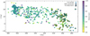 |
Fig. 1 Input sample of K-type pre-main-sequence stars in Sco-Cen. We show the sky positions of the targets in galactic coordinates and the color of the markers indicates the distance to the objects. Members of the YSES subsample are highlighted by the black outlines around the markers. The star highlights TYC 8252-533-1, whose brown dwarf companion is analyzed in Sect. 4.1. |
Candidate triple systems to K-type stars in Sco-Cen.
Candidate companion systems with complementary SPHERE data from YSES.
2.3 High-contrast imaging observations
Seven of our preselected companion candidates were also imaged with SPHERE as part of YSES. The identifiers of these systems are listed in Table 2. For a potential brown dwarf companion around TYC 8252-533-1, we collected additional data with NACO (Lenzen et al. 2003; Rousset et al. 2003) at ESO’s Very Large Telescope. A detailed overview of all observations and the weather conditions is provided in Table B.1. The reduction is detailed in Bohn et al. (2020a), with a custom processing pipeline that is based on version 0.8.1 of the PynPoint package (Stolker et al. 2019). As the companions are reasonably bright and widely separated from the star, we did not perform any PSF subtraction when evaluating their astrometry and photometry.
3 Gaia results and analysis
In this section, we analyze the results that were derived from our preselection described in Sect. 2.1. In Sect. 3.1, we show the object magnitudes of identified candidate companions as a function of angular separation with respect to the primary star. As we know the ages of all our targets, we can convert these flux measurements to mass estimates for the companion candidates. This analysis is detailed in Sect. 3.2. We further assess the colors of our candidate companions and evaluate whether these are consistent with the proposed Sco-Cen membership in Sect. 3.3. We analyze the relative motions of all identified objects and probe if these are in agreement with a gravitationally bound orbit around the primary star. This assessment is presented in Sect. 3.4. In Sect. 3.5, we present the properties of the candidates that exhibit the highest likelihood of being bound companions.
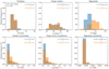 |
Fig. 2 Astrometric and photometric properties of the input sample along with the preselected list of candidate companions (CCs). In the top panel, we present the distributions of the object parallaxes, proper motions, and magnitudes from both samples. In the lower panel, the uncertainties are shown. The colored values in the upper right of each panel indicate the median and the 68% confidence intervals of the associated distributions. |
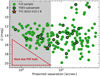 |
Fig. 3 Identified companion candidates to K-type Sco-Cen members. Members of the YSES subsample are highlighted by the black outline around the marker. The orange star highlights the brown dwarf companion TYC 8252-533-1 B that is analyzed in Sect. 4.1. The apparent Gaia G band magnitude is presented as a function of projected separation in arcseconds. Due to the PSF halo of the primary, the detectable magnitude threshold increases with larger separations from the host. This area of reduced sensitivity is indicated by the red, dashed triangle. The gray-shaded region represents the field of view of the SPHERE/IRDIS detector. |
3.1 Raw Gaia astrometry and photometry
In Fig. 3, we present the apparent G band magnitudes of the identified companion candidates as a function of projected separation. The detection sensitivity improves with increasing separation from the target, which can be attributed to the PSF halo of the host star. There is a clear exclusion zone (as indicated by the red, dashed triangle in Fig. 3) in which the presented technique is not able to detect any low mass comoving objects. This region is however highly complementary to the parameter space that is covered by the field of view of current generation of high-contrast imaging instruments. The gray-colored background of Fig. 3 shows the field of view of the SPHERE/IRDIS camera with a radial extent of ≤5′′.5. The seven companions that were observed within the scope of YSES are located in this part of the parameter space. For separations that are larger than approximately 10 arcseconds, the Gaia contrast to the primary becomes background limited and we are sensitive to objects with an apparent G band magnitude down to 20 mag. This is in good agreement with the limiting magnitude of G = 21 mag that is required for objects to appear with a five-parameter astrometric solution in the EDR3 catalog (Gaia Collaboration 2021).
3.2 Mass estimation
To characterize the identified companion candidates in further detail, we determined the absolute magnitudes of the objects using the parallax measurement provided by Gaia EDR3. In many cases, the parallaxes of the identified companion candidates have larger uncertainties than the parallax measurements of the stars from our input catalog, which have a median error of only 0.02 mas (see Fig. 2). We therefore used the latter parallax values to estimate the distances to the detected objects. Even though this requires true companionship between both objects, this estimate is a reasonable assumption as all candidate companions are Sco-Cen members, according to the astrometric membership criteria from de Zeeuw et al. (1999) and Pecaut & Mamajek (2016) (see Sect. 2.1). As Pecaut & Mamajek (2016) provide age estimates6 for all systems but one, we converted the absolute magnitudes of the companions to object masses by evaluation of BT-Settl models (Allard et al. 2012; Baraffe et al. 2015) at the corresponding system age. The remaining system without an age measurement, SZ 65 (2MASS J15392776-3446171, Gaia EDR3 6013399894569703040), is a member of the Lupus star forming region, so we assigned it an age of 2 Myr in accordance with the average age of this cloud complex (Comerón 2008; Alcalá et al. 2014). For all ages we assumed an uncertainty of 2 Myr with a youngest possible age of 1 Myr. The BT-Settl models we used are valid for objects with masses smaller than 1.2 M⊙, which is equivalent to an apparent G band magnitude of approximately 11 mag at the average distance of Sco-Cen and at an age of 15 Myr. For the brightest objects from Fig. 3, which were outside the magnitude range supported by the BT-Settl models, we used MIST isochrones (Dotter 2016; Choi et al. 2016) to convert their G band photometry to a stellar mass. As the object masses strongly depend on the underlying system age and only a single photometric measurement is used for the derivation, we do not claim that the provided mass estimates are very precise, but instead indicate whether it is a brown dwarf or a stellar companion. The derived mass estimates for the companion candidates are listed in Table C.1.
We present the companion masses as a function of projected physical separation in Fig. 4. The conversion from projected angular separations to projected physical separations was performed using the distance estimate based on the parallax measurement of the primary. We do not include the difference in Gaia parallaxes between primary and companion to determine a three-dimensional separation, as these measurements have typical errors of 0.02 mas and 0.05 mas for stars from our input catalog and companion candidates, respectively (see Fig. 2). For two average Sco-Cen members with parallaxes of 7.5 mas, Gaussian error propagation provides an uncertainty for the radial separation on the order of 1 pc or approximately 200 000 au. This uncertainty is much larger than our measured projected separations and would dominate the uncertainty of the derived parameter. We proceeded to use projected separations as a lower limit for the three-dimensional distances.
In Fig. 4, the region of limited sensitivity due to the PSF halo of the primary is still clearly visible and it implies thatfor separations closer than approximately 300 au, we are only sensitive to stellar-mass companions. Farther away from the host, however, we can detect comoving brown dwarf companions with masses smaller than 80 MJup. The lower mass threshold is reached for separations larger than approximately 1000 au and we are sensitive to objects masses as low as 20 MJup. Exoplanets at Sco-Cen distance and age and with masses below the deuterium burning limit of approximately 13 MJup are thus marginally too faint to be confidently detected with Gaia EDR3.
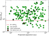 |
Fig. 4 Identified companion candidates to K-type Sco-Cen members II. Members of the YSES subsample are highlighted by the blackoutline around the marker. The orange star highlights TYC 8252-533-1 B analyzed in Sect. 4.1. The companion mass is presented as a function of projected separation in Astronomical Units. Mass conversion was performed by comparison to BT-Settl and MIST models evaluated at the system age. The dashed red line at 80 MJup indicates the threshold between brown dwarfs and stellar mass companions. |
3.3 Color-magnitude analysis
To confirm the young and (sub-)stellar nature of the detected objects, we evaluated all candidate companions in a color-magnitude diagram as presented in Fig. 5. The color is estimated using the Gaia filters for the blue (GBP) and red part (GRP) of the G band continuum. As visualized in Fig 5, most of the candidate companions have colors that are in very good agreement with synthetic MIST and BT-Settl models for young objects of 15 Myr, which is a reasonable average for the presented Sco-Cen sample (Pecaut & Mamajek 2016). This corroborates the Sco-Cen membership of the analyzed candidates and each of these is very likely to be a young member of the association, even if it turns out not to be a companion to any of the stars from our input catalog. There are two outliers at the faint end of the sequence that appear to be bluer than predicted by the evolutionary models. This is, however, not a contradiction with Sco-Cen membership of these objects. The corresponding objects, Gaia EDR3 5232514298301348864 and Gaia EDR35997035416337166976, are the faintest among our full sample of identified companion candidates with a G band magnitude of 19.9 mag and 19.3 mag, respectively. Their GBP and GRP photometric measurements exhibit a corrected flux excess factor C* of 0.62 and0.28, respectively, which is different from the value of C* =0 that is associatedwith trustworthy photometry (Riello et al. 2021). This large uncertainty most likely originates from the faint GBP flux of the objects, whose true value might be below Gaia’s sensitivity limits in this channel. Hence, it is certainly possible that Gaia EDR3 5232514298301348864 and Gaia EDR3 5997035416337166976 are much redder than indicated in Fig. 5 and consistent with the colors that are predicted for a low-mass brown dwarf companion at Sco-Cen age. This conclusion is corroborated by the better-constrained G − GRP colors of both objects. These values of 1.5 mag and 1.3 mag are in good agreement with late M spectral types.
It should be noted that not all of our identified companion candidates have GBP and GRP flux measurements, as can be seen in Table C.1. These 27 targets without any color information are not included in the plot shown in Fig. 5 and their photometric Sco-Cen membership compatibility thus cannot be assessed properly. For 23 of these insufficiently characterized companions the lack of precise color measurements is explained by their proximity and contrast with respect to the target star. All of these objects exhibit angular separations of less than 3′′. The remaining four candidates without any color information are at larger separations from the target star, but in all cases these have an additional Gaia source of equal or higher brightness at very close separations (< 2′′); these are most likely affecting the flux measurements. For Gaia EDR3 6022499010440068864 and Gaia EDR3 6208381587215253504 these close contaminants are members of the same candidate multiple systems that we have preselected.
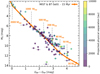 |
Fig. 5 Color-magnitude diagram of identified companion candidates to K-type stars in Sco-Cen. The colors of the markers indicate the projected separation between host and companion. The orange line represents a combination of MIST and BT-Settl isochrones for an age of 15 Myr. |
3.4 Companionship assessment
We further analyzed whether the identified companion candidates are gravitationally bound multiple systems based on the available astrometric data. In the general description of the gravitational two-body problem, a system is considered bound when its total kinetic energy, namely:
 (1)
(1)
is smaller than the potential energy,
 (2)
(2)
of both bodies. In this formalism, r denotes the separation of the two bodies; ṙ and  are the radial and azimuthal velocities with respect to the center of mass. The sum of both individual object masses M1 and M2 is M and we define the reduced mass as:
 (3)
(3)
These conditions imply that a gravitationally bound system requires
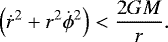 (4)
(4)
Even though we do not know the objects’ true three-dimensional separations and differential velocities, Eq. (4) allows us to assess which systems cannot be bound. This is possible because our projected differential velocity vproj is strictly smaller or equal to the amplitude of the true differential velocity  . Likewise, the right-hand side of Eq. (4) is bound from above by substituting r in the expression with our measured projected separation ρ ≤ r as
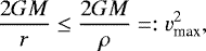 (5)
(5)
where we defined this new expression as the maximum allowed differential velocity for a system to be bound.
Hence, we evaluated the ratio of our measured projected velocity difference vproj and vmax to assess whichsystems are most likely not bound as per:
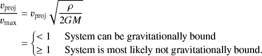 (6)
(6)
This expression is completely symmetric in M1 and M2, so within this formalism it does not matter which star is considered to be the primary of the system. While a ratio greater than or equal to one is a good indicator that the studied system cannot be physically bound, a value smaller than unity does not necessarily indicate that the opposite scenario is true, due to the unknown contributions to the separation and differential velocity along our line of sight. This metric is valid for regular binary systems, but it is not suitable for assessing systems with higher orders of multiplicity, such as the potential triple systems we found around some of our targets. A proper treatment for these special cases, however, is not straightforward and will thus be neglected in our further analysis. The fraction of triple or higher-order multiple systems is assumed to be approximately 25% among solar-type multiple systems (e.g., Mayor & Mazeh 1987; Eggleton & Tokovinin 2008; Duchêne & Kraus 2013). It is thus not surprising that we have identified 21 candidate triple systems out of 142 candidate multiples from our preselection. This smaller fraction of ≈15% does not violate these statistical constraints as some triple systems will certainly be missed either due to the cutoff separation or additional components below the resolution limit of Gaia.
We calculated the differential proper motions between target and companion from the values listed in the Gaia EDR3 database (see Appendix C). To convert this angular movement to a differential projected velocity vproj in km s−1, we used the inverted parallax of the star from our input catalog. For the derivation of vmax, we adopted the mass measurements for the stars of our sample from Pecaut & Mamajek (2016). For SZ 65, which was lacking in a value for this in Pecaut & Mamajek (2016), we used a mass of 0.7 M⊙ based on previous work by Alcalá et al. (2017). The masses of the identified companions were estimated as previously determined by Gaia photometry and for the objects that were heavier than the maximum valid mass from our BT-Settl models we used MIST isochrones to derive a stellar mass.
The resulting ratios of vproj to vmax that we derived for all objects are listed in Table C.1. The error budget in the calculation of these quantities is dominated by the uncertainty of the differential velocities of both objects. The uncertainties of vproj ∕vmax were propagated by a bootstrapping approach. We repeated the velocity calculation 10 000 times, drawing the initial proper motions of both objects from Gaussian distributions that are centered around the Gaia EDR3 values, and their corresponding uncertainties served as standard deviation for these initial normal distributions. The derived vproj to vmax ratios represent the median of the corresponding posterior distribution and the surrounding 68% confidence interval as an estimate of the uncertainties. We visualize these derived parameters as a function of angular separation and companion mass in Fig. 6.
Most of the identified companion candidates are consistent with vproj ∕vmax < 1, which indicates that for these objects a gravitationally bound orbit is not ruled out by Gaia EDR3 data. To quantify the likelihood of these objects to be a real companion to the target of our sample, we derive the probability of a vproj to vmax ratio that issmaller than unity, based on our 10 000 samples for each posterior distribution. This value  represents an upper limit for the dynamical companionship probability, since the complete three dimensional astrometry of all objects is not available.
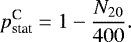
As this value does not account for comoving Sco-Cen members that might have similar projected velocities as a target from our input catalog despite not being gravitationally associated, we further derived a statistical companionship likelihood  . For each companion candidate we checked how many sources were found by our preselection algorithm, when choosing a cutoff separation that is twenty times as large as the projected separation of the candidate (see e.g., Fontanive & Bardalez Gagliuffi 2021). This number provides an estimate of how many other Sco-Cen objects with similar parallaxes and proper motions are in the immediate surroundings of the stars from our input catalog. We obtained the adjusted number of objects, N20, by counting the objects within the twenty times larger reference region while excluding the originally enclosed companion candidates. Based on this number we derived a statistical probability of having one of these sources in the 400 times smaller search region. The statistical companionship likelihood is then calculated as:
 (7)
(7)
Our final companionship probability considers both these dynamical and statistical terms and is derived as:
 (8)
(8)
These values are provided in Table C.1.
We find that only 27%, 31%, and 33% of our identified companion candidates have a pC value that is smaller than 0.1, 0.5, and 0.95, respectively. Even though the true membership probabilities might be lower than the values we have derived here, this test strongly suggests that our preselection based on Gaia astrometry is a viable method for detecting comoving companions to stars that have their position and proper motion measurements listed in Gaia EDR3.
We did not detect any trends of objects without any color measurement having significantly higher likelihoods to be unbound. This is expected as the missing color information does not arise from the companion candidates but by the proximity to another object of equal or higher brightness. The majority of the aforementioned 23 companions without color data that are closer than 3′′ to the target star from our input catalog exhibits pC > 0.5 and 19 out of these even pC > 0.95. As expected, due to their small projected separations of less than 300 au, these are very likely to be gravitationally bound stellar binaries. Only three objects without color measurements at separations that are smaller than 3′′ are found to have pC < 0.1.
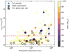 |
Fig. 6 Relative velocities of identified companions of a sample of K-type Sco-Cen members. We show the ratio of the differential projected velocities vproj to the maximum velocity that allows a gravitationally bound system vmax as defined in Eq. (6). This parameter is a measure of whether our preselected candidate companions are part of a binary system; a value greater than unity renders this scenario as unlikely. These two different regimes are separated by the dashed red line. The colors of the markers indicate the mass of the corresponding candidate companion. To focus primarily on the sub-stellar objects in our sample the color bar is cut off at masses that are higher than 100 MJup. Markers with a black outline refer to members of the YSES subsample and TYC 8252-533-1 B is highlighted by the star. |
3.5 High confidence companions
When applying a conservative cutoff of pC > 0.95 to the full list of preselected companion candidates, 110 objects around 104 targets have a high probability of being gravitationally associated with the star from the input catalog. A detailed list of these high confidence companions and their main parameters is presented in Table C.2. For each system, we designated the object with the brightest G band magnitude to be the primary. The six remaining triple systems in this list are represented by two individual entries each and we derived all properties with respect to the primary.
The masses and separations of these high confidence binaries are presented in Fig. 7. The majority of the companions exhibit projected separations that are smaller than 1000 au. We find a median separation of  au and no companion is farther separated than 7000 au. The peak of the separation distribution is located at approximately 50 au, which is in good agreement with general binary statistics (e.g., Duchêne & Kraus 2013). For the masses of the companions, we derived a median value of
  , which is well within the M dwarf regime. More massive and less massive objects are less frequent among the high confidence companions.As shown in Fig. 3, this statistical evaluation does not consider close-in, low-mass companions that are below the sensitivity of our detection method. The derived median mass might thus be biased for these missing objects. Nevertheless, our results agree well with the findings of Duquennoy & Mayor (1991) and Raghavan et al. (2010), who established a peak in the companion mass ratio distributions to solar-type primaries at q ≈ 0.3 and q ≈ 0.1, respectively.
We identified ten sub-stellar objects with masses below 80 MJup that are very likely to be comoving with pC > 0.95. The identifiers and mass estimates for these brown dwarf companions are listed in Table 3. The most intriguing of these are: Gaia EDR3 5232514298301348864, Gaia EDR3 6039427503765943040, and Gaia EDR3 6043486655875354112, which exhibit masses below 40 MJup. The latter is not too far away from the planetary mass regime with a photometric mass estimate of 24.8 ± 1.0 MJup. Except for Gaia EDR3 5860803696599969280, which was reported in Goldman et al. (2018), these are all newly identified brown dwarf members of Sco-Cen. Their likely companionship to K-type stellar members of this association makes these especially intriguing laboratories not only for spectroscopic follow-up observations but also for studies of the dynamical evolution of multiple systems in a densely populated stellar birth environment. While the former will allow us to understand the atmospheric architectures and compositions of these sub-stellar objects, the latter will provide important implications for companion migration and ejection mechanisms caused by close stellar encounters.
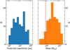 |
Fig. 7 Properties of high-confidence companions to K type Sco-Cen members. Left panel: distribution of separations amongst our high confidence sample. Right panel: mass distribution among this sample. The red dashed line indicates the threshold of brown dwarf and stellar-mass companions at 80 MJup. |
Brown dwarf companions companions with pC > 0.95.
4 High-contrast imaging results
In this section, we present the results from our high-contrast imaging observations with SPHERE and NACO that were obtained within the scope of YSES. Section 4.1 contains a detailed analysis of a brown dwarf companion that we detected to TYC 8252-533-1. We briefly assess the astrometry and photometry of other companions in the SPHERE field of view detected to other YSES targets from our input catalog in Sect. 4.2.
4.1 Brown dwarf companion to TYC 8252-533-1
Our previous analysis revealed that the YSES target TYC 8252-533-1 (2MASS J13233587-4718467; Gaia EDR36083750638577673088) harbors a companion with a projected separation of 4′′.4 and at a position angle of 204°. As Gaia photometry suggests that the companion is of sub-stellar mass and likely a brown dwarf companion, we refer to it as TYC 8252-533-1 B henceforth. Due to the small angular separation of the binary, both objects were located within the SPHERE field of view during our regular YSES observations. This object is thus an ideal test case to assess the quality of the parameters that were derived from the Gaia catalog by comparison to independent photometry and astrometry acquired with SPHERE. To characterize this companion independently from the Gaia measurements, we acquired SPHERE dual-band measurements ranging from Y to K band and additional NACO L′ data as described in Sect. 2.3. The final images for several SPHERE filters and our NACO data are presented in Appendix B.
4.1.1 Stellar parameters
A summary of the basic stellar parameters of TYC 8252-533-1 is presented in Table 4. To convert the photometric contrasts measured in the SPHERE and NACO data into absolute fluxes, it was necessary to characterize the primary star first. We analyzed its spectral energy distribution (SED) with VOSA (Bayo et al. 2008) using flux measurements from Tycho (Høg et al. 2000), APASS (Henden et al. 2012), Gaia EDR3 (Gaia Collaboration 2021), DENIS (DENIS Consortium 2005), 2MASS (Skrutskie et al. 2006; Cutri et al. 2003), and WISE (Cutri et al. 2012b). Pecaut & Mamajek (2016) measured an extinction of AV = 0.16 mag and reported that the star is likely to host a debris disk based on the infrared excess that was observed in WISE W3 and W4 filters. The STILISM reddening map (Lallement et al. 2014) provides a total visual extinction of AV = (0.05 ± 0.05) mag at the position and distance of our target. We therefore allowed extinctions in the range 0 mag < AV < 0.2 mag and excluded the W3 and W4 measurements from the fit of the stellar SED.
As the stellar flux measurements of the primary might be affected by flux from the close companion, we briefly assessed the extent of this potential contamination. The fractional contribution from the secondary to the measured flux of the primary is maximized for the longest wavelengths of the analyzed SED7. Equation (2) of Bohn et al. (2020c) yields a contribution of 0.04 mag to the stellar magnitude in L′ band if the binary was unresolved in the photometric data. This contribution is significantly smaller for shorter wavelengths, where the contrast between both objects is larger. We therefore did not perform any correction of the flux measurements for the primary, as the contribution from the secondary is below 5% and is thus already considered in the larger uncertainties of the magnitude contrast values (as presented in Table 5) when deriving the fluxes of the companion.
The stellar distance was fixed to 130 pc using the estimate from Bailer-Jones et al. (2021) based on Gaia EDR3 parallaxes, and we assumed a solar-like metallicity of the primary. We fitted a grid of BT-Settl models (Allard et al. 2012; Baraffe et al. 2015) in a χ2 minimizing approach, and the best fit of the data was provided by a model with an effective temperature of Teff = 4500 ± 50 K, a surface gravity of  , a stellar luminosity of
  , and a visual extinction parameter of AV = 0.13 ± 0.06 mag. These values are in good agreement with the properties that Pecaut & Mamajek (2016) derived for TYC 8252-533-1.
Properties of TYC 8252-533-1.
De-reddened photometry of TYC 8252-533-1 and its brown dwarf companion.
Relative astrometry of TYC 8252-533-1 B with respect to the primary.
4.1.2 Brown dwarf astrometry
To assess whether our high-contrast data confirm a bound orbit of TYC 8252-533-1 B, we extracted the relative astrometry with respect to the primary star for all of our observations. For SPHERE, we used the general astrometric solution presented in Maire et al. (2016) with a true north correction of − 1°.75 ± 0°.08 and plate scales of 12.255 mas px−1, 12.251 mas px−1, and 12.265 mas px−1 for H2, H, and Ks band images, respectively. The NACO data were calibrated with a plate scale of 27.193 ± 0.059 mas px−1 (Launhardt et al. 2020) but no true north correction was applied as discussed in Bohn et al. (2020a). The derived separations and position angles are presented in Table 6 and visualized in Fig. 8. The measurements clearly confirm that the path of TYC 8252-533-1 B is highly inconsistent with the simulated trajectory of a static background object. Instead, the relative astrometric offsets with respect to the primary are in good agreement with the small relative velocity that is expected from an orbit with a projected angular separation of approximately 570 au. Even though there are still some systematic sources of uncertainties between the astrometric measurements that originate from different instruments or filters, the high-contrast imaging data clearly confirm the hypothesis, based on the Gaia data, that TYC 8252-533-1 B is a bound companion to the solar-type primary TYC 8252-533-1.
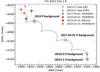 |
Fig. 8 Proper motion analysis of TYC 8252-533-1 B. The colored markers represent the relative offsets in RA and Dec with respect to the primary that we measured in SPHERE and NACO imaging data or derived from the Gaia DR2 and EDR3 catalogs. The blue dashed line illustrates the trajectory of a static background object at infinity and the white markers along the curve represent the hypothetical positions of such an object at the epoch of the corresponding observation. |
4.1.3 Brown dwarf photometry
The de-reddened photometry of TYC 8252-533-1 B and its host star are presented in Table 5. The listed Gaia photometry is directly obtained from the EDR3 catalog and the infrared photometry originates from our high-contrast imaging data. We applied the previously determined extinction of AV = 0.13 mag to correct the presented fluxes. As the SPHERE H band data from 2017-04-02 were collected in poor atmospheric conditions and with a very unstable AO performance, we disregarded the photometry that was extracted from these observations in our further analysis. We fitted the full optical and infraredSED of the companion utilizing the MCMC approach described in Bohn et al. (2020b). We used a linearly interpolated grid of BT-Settl models (Allard et al. 2012; Baraffe et al. 2015) with effective temperatures, Teff, between 1500 K and 4000 K, surface gravity in the range of  , and solar metallicity. We further allowed object radii R from 0.5 RJup to 5 RJup. The MCMC sampler was implemented in the emcee framework (Foreman-Mackey et al. 2013) and we used 100 walkers with 10 000 steps to sample the posterior distribution. In accordance with the computed autocorrelation time of approximately 200 steps, the first 1000 samples of each chain were discarded as burn-in phase and we further continued using each twentieth step of the remaining chains. This provided 45 000 samples for our posterior distribution in (Teff,
  , R), which are visualized in Fig. D.1. From these distributions we derived an effective temperature of
  , a surface gravity of
  dex, and a radius of
  for TYC 8252-533-1 B. These values were obtained as the 95% confidence intervals around the medians of the posterior distributions. From these three parameters we derived the object luminosity as
  . The results of this SED fit are presented in Fig. 9. Interestingly, the derived object radius is markedly larger than usual radii of field brown dwarfs of this mass, which are on the order of 1 RJup (e.g., Chabrier et al. 2009). This inflated photometric radius, however, is nothing unusual for sub-stellar companions at this young age, and similarly large values have been reported for various planetary-mass objects (e.g., Schmidt et al. 2008; Bohn et al. 2019; Stolker et al. 2020).
To convert the results of this analysis to a mass estimate for the companion, we assumed a system age of 5 ± 2 Myr (Pecaut & Mamajek 2016). The kinematic parallax that Pecaut & Mamajek (2016) used for this target (7.83 mas) is not far from the Gaia EDR3 value of 7.71 mas. The difference in age due to the different adopted distances should therefore be considered in our assigneduncertainties. Evaluation of BT-Settl isochrones at this age and with our derived luminosity yielded a mass of  for TYC 8252-533-1 B, which makes it likely a brown dwarf companion to the solar-type primary. This value is in good agreement with the photometric mass estimate of 48.7 ± 11.1 MJup that is derived from the Gaia G band flux.
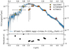 |
Fig. 9 SED of TYC 8252-533-1 B. The yellow, orange, and red squares indicate the photometry we measured for Gaia, SPHERE, and NACO filters, respectively. The bars in the x direction indicate the width of the filter transmission curves. The blue curve presents the median model from our posterior distribution of the SED fit as shown in Fig. D.1. We present the integrated flux of this median model in the applied filters with the grey squares and we visualize 100 randomly selected models from our posterior distribution as grey curves. In the bottom panel, we present the residuals of the fit. |
4.1.4 System architecture
Based on the observed infrared excess in the W3 and W4 filters, the primary star likely hosts a debris disk (Pecaut & Mamajek 2016, and Sect. 4.1.1). Our direct imaging data do not reveal any scattered light flux of this postulated debris ring, which is most likely below the detection sensitivity of our total intensity observations. Nevertheless, we assessed the relative location of this newly identified brown dwarf companion with respect to the circumstellar material. As our photometric data cover only wavelengths shorter than 22 μm (W4), we most likely do not sample the peak of the infrared excess emission; hence, we could only derive an upper limit for the temperatureof the dust grains in the disk. We assumed a single species of dust grains that is located at a radial separation, rdust, from the central star, and modeled the thermal dust emission by a single blackbody with a dust temperature Tdust. As the peak of this emission is detected either in W4 or at longer wavelengths, we could constrain a maximum dust temperature of Tdust ≤ 130 K. We converted this dust temperature to a minimum disk radius of rdust ≥ 4 au, utilizing a temperature-radius relation as presented by Backman & Paresce (1993) with
 (9)
(9)
where L* denotes our previously determined stellar luminosity. Even though this lower limit does not rule out that the debris disk around the primary might extend up to a separation that is on the order of the projected separation of 570 au that we measure for TYC 8252-533-1 B, this scenario is expected to be extremely unlikely, as it would require dust temperatures as low as 10 K. In agreement with temperature and radius measurements from other debris disk studies that rely on either SED modeling (e.g., Moór et al. 2011) or spatially resolved imaging of these environments (e.g., Pawellek et al. 2014), we conclude that TYC 8252-533-1 B is thus very likely located outside the debris disk of its primary star.
TYC 8252-533-1 B is a new data point to the catalog of debris-disk systems that are harboring giant exoplanets or brown dwarf companions such as HR 8799 (Marois et al. 2008, 2010), β Pictoris (Lagrange et al. 2009, 2010), HD 95086 (Rameau et al. 2013), HD 106906 (Bailey et al. 2014), HR 3549 (Mawet et al. 2015), HR 2562 (Konopacky et al. 2016), or HR 206893 (Milli et al. 2017). While the giant companions HR 8799 bcde, β Pic b, HD 95086 b, HR 2562 B, and HR 206893 B are located inside the debris disks of their host stars, HD 106906 b, HR 3549 B, and TYC 8252-533-1 B reside beyond them. Whereas the objects in the former category might have formed via core accretion (Pollack et al. 1996; Alibert et al. 2005; Dodson-Robinson et al. 2009; Lambrechts & Johansen 2012) or gravitational instabilities in the protoplanetary disk (Boss 1997, 2011; Rafikov 2005; Durisen et al. 2007; Kratter et al. 2010), similar formation mechanisms are unlikely for the objects that are found outside the circumstellar disks of their hosts, as in situ formation at these large separations is not supported by these mechanisms, and migration from within the current disk is unlikely without disrupting the circumstellar environment (Raymond et al. 2012). As concluded by Bailey et al. (2014) for HD 106906, it is thus likely that TYC 8252-533-1 B rather formed via a star-like pathway by fragmentation processes in the collapsing protostellar cloud (Kroupa 2001; Chabrier 2003). Future astrometric observations to constrain the orbital parameters of this brown dwarf and spectroscopic analysis of its atmospheric composition are required to confirm this suggested formation scenario.
4.2 Stellar companions in the SPHERE field of view
Six additional companion candidates from the Gaia preselection were also identified in the SPHERE observations that were collected within the scope of YSES. Contrary to TYC 8252-533-1 B, most of these companions seem to exhibit masses that are in good agreement with stellar nature of these objects. In this section, we briefly assess the combined SPHERE and Gaia astrometry and photometry of these objects. The numerical values are presented in Table 7. We used 2MASS JHK photometry of the systems to derive the absolute magnitudes for the companion candidates. For 2MASS J12195938-5018404, 2MASS J12505143-5156353, and 2MASS J12560830-6926539, the Gaia companion candidates are spatially resolved by 2MASS, so they should not pollute the flux measurement of the primary. This is not the case for 2MASS J12391404-5454469, 2MASS J13130714-4537438, and 2MASS J13335481-6536414, for which the fluxes of both sources are blended. Furthermore, we identified an additional companion candidate at a separation of approximately 0′′.2 to 2MASS J12560830-6926539, which is resolved neither by 2MASS nor Gaia. To obtain an unbiased estimate for the flux of the primary star, we corrected the 2MASS magnitudes of these unresolved pairs for the additional contribution, utilizing Eq. (2) from Bohn et al. (2020c). These revised values are reported in Table 7. As for the Gaia fluxes, the SPHERE photometric measurements were converted to object masses by BT-Settl models that were evaluated at the system age. The corresponding imagery for these additional companions is shown in Fig. B.2.
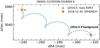 |
Fig. 10 Proper motion analysis of 2MASS J12195938-5018404 B. See Fig. 8 for a detailed description of the plot elements. |
4.2.1 2MASS J12195938-5018404
The candidate companion detected to 2MASS J12195938-5018404 clearly seems to be stellar in nature. While the Gaia G band photometry indicates an object mass of 464.7 ± 29.3 MJup, the SPHERE near-infrared photometry favors slightly lower masses of approximately 375 MJup. Both measurements are consistent at the 2σ level, and the slightly higher Gaia value might originate from uncorrected flux contribution of the primary star. As illustrated in Fig. 10, SPHERE and Gaia astrometry for the companion candidate are highly consistent. This is also supported by a companionship probability of pC = 100%, as derived from Gaia astrometry alone. We thus conclude that 2MASS J12195938-5018404 B is a stellar secondary to its solar-mass primary. The binary has a projected separation of approximately 470 au.
4.2.2 2MASS J12391404-5454469
The companion candidate to 2MASS J12391404-5454469 is supposedly of a stellar mass. The Gaia photometry is consistent with a mass of 189.1 ± 41.9 MJup. Again, the SPHERE data favor a smaller object mass of approximately 110 MJup. The proper motion analysis clearly supports that the companion candidate is gravitationally bound to the primary star, and has a projected separation of approximately 275 au (see Fig. 11). This combined astrometric analysis is confirmed by pC = 100% that was derived from Gaia data alone. We thus refer to the object as 2MASS J12391404-5454469 B henceforth.
4.2.3 2MASS J12505143-5156353
The three mass estimates derived from the SPHERE H and Ks band and Gaia G band data agree particularly well for the candidate companion to 2MASS J12505143-5156353. As presented in Fig. 12, the object is clearly comoving with the primary star. The Gaia companionship probability of pC = 100% that we derived for this object strongly supports this conclusion. It should therefore be named 2MASS J12505143-5156353 B, a stellar companion with a mass of approximately 185 MJup. The projected separation between primary and secondary is approximately 350 au.
SPHERE astrometric and photometric measurements of stellar companions identified by the Gaia search.
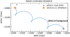 |
Fig. 11 Proper motion analysis of 2MASS J12391404-5454469 B. See Fig. 8 for a detailed description of the plot elements. |
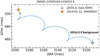 |
Fig. 12 Proper motion analysis of 2MASS J12505143-5156353 B. See Fig. 8 for a detailed description of the plot elements. |
 |
Fig. 13 Proper motion analysis of 2MASS J12560830-6926539 B. See Fig. 8 for a detailed description of the plot elements. |
4.2.4 2MASS J12560830-6926539
As presented in Fig. 13 the astrometry from Gaia and SPHERE for the candidate companion to 2MASS J12560830-6926539 clearly disfavors a static background object. However, the relative astrometric measurements for both epochs are too disjuncted to allow for a bound orbit withinthe measurement uncertainties. This conclusion seems to be supported by a velocity ratio of vprojvmax = 1.36 ± 0.06 and a Gaia companionship probability of pC = 0%.
The reason for this inconsistency can be identified in the high-contrast imaging data collected on 2MASS J12560830-6926539 (see Fig. B.2). The primary star is resolved into a visual binary with an angular separation of 0′′.218 ± 0′′.006. The fainter of the two stars is detected at a position angle of 33°.8 ± 1°.6. The binarity of the source was identified within the scope of the Search for associations containing young stars (SACY; Torres et al. 2006; Elliott et al. 2015) and confirmed by Tokovinin et al. (2019). It also affects the accuracy of the provided Gaia astrometry. The Gaia measurements exhibit an astrometric excess noise of 2.3 mas (astrometric_excess_noise parameter) that is detected at a significance of approximately 6 820 (astrometric_excess_noise_sig parameter). This significance is much larger than the threshold of 2 that is required for a certain corruption of the astrometric measurements (see Lindegren et al. 2021b). This conclusion is also supported by a renormalised unit weight error (RUWE) of ~ 13; for well-behaved sources, a value of RUWE ≈ 1 is expected. As parallaxes and proper motions for the binary and the Gaia companion candidate are highly consistent, it is very likely that these three objects form a gravitationally bound triple system. Further astrometric monitoring will help to confirm this hypothesis.
The companion candidate from Gaia was spectroscopically analyzed by Riaz et al. (2006). The authors determined a spectral type of M1 and classified it as a stellar object. This is in stark contrast to the photometric mass estimates that we derived from both Gaia and SPHERE. The Gaia G band photometry is consistent with a mass of 44.5 ± 5.8 MJup and the SPHERE H and Ks band data indicate object masses of  and
and  , respectively. These values are consistent within their uncertainties and suggest that Gaia EDR3 5844909156504880128 (2MASS J12560892-6926503) is a brown dwarf rather than a stellar companion. It is possible that Riaz et al. (2006) misclassified the companion, perhaps due to contaminating flux from the primary star that was leaking into the slit (with a width of 1′′.5). Further spectroscopic measurements will help to confirm the sub-stellar nature of this outer companion in a young triple system.
 |
Fig. 14 Proper motion analysis of 2MASS J13130714-4537438 B. See Fig. 8 for a detailed description of the plot elements. |
4.2.5 2MASS J13130714-4537438
The Gaia and SPHERE astrometric measurements for the companion candidate to 2MASS J13130714-4537438 are highly consistent and indicate that this object is gravitationally bound to its Sun-like primary (see Fig. 14). This conclusion was also drawn from Gaia astrometry alone, for which we calculated pC = 100%. We derived photometric mass estimates of 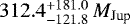 and
and 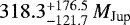 from the SPHERE H and Ks band data, respectively. The corresponding Gaia mass of 414.4 ± 114.2 MJup is marginally higher, but fully consistent within the uncertainties. These mass errors are relatively large for this object. Due to the young age of the system of
  Myr, the object mass can vary significantly when propagating the age uncertainties. 2MASS J13130714-4537438 B is likely a stellar-mass companion at a projected separation of approximately 100 au.
4.2.6 2MASS J13335481-6536414
As illustrated in Fig. 15, the three astrometric data points collected with SPHERE and Gaia are in very good agreement with each other. This analysis and the Gaia companionship probability of pC = 100% strongly support that 2MASS J13335481-6536414 B is a gravitationally bound companion with a projected separation of approximately 140 au. Both opticaland near infrared photometric mass estimates for the secondary agree very well within their uncertainties. While the photometricmass estimate from Gaia suggests that 2MASS J13335481-6536414 B is a low-mass stellar object with a mass of 91.9 ± 31.0 MJup, the SPHERE data indicate that it might be of sub-stellar nature with a mass of approximately 78 MJup. However, the upper boundaries of the SPHERE measurements also allow for the estimation of stellar masses. Future data will be required to discern whether 2MASS J13335481-6536414 B is a high-mass brown dwarf or, rather, a low-mass stellar companion.
An additional companion candidate to 2MASS J13335481-6536414, at a projected separation of more than 1000 au, was detected by the Gaia preselection algorithm. For this object, with the identifier Gaia EDR3 5863747467220738432, we derived vprojvmax = 1.32 ± 0.02 and, hence, pC = 0%. It is possible that the visual stellar binary of 2MASS J13335481-6536414 AB is corrupting the astrometric measurements for the primary. Further monitoring will be necessary to determine the orbital parameters of this binary. These data will be helpful to assess whether the additional companion candidate is consistent with a bound orbit after all and was just rejected due to the velocity contribution from the inner binary.
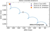 |
Fig. 15 Proper motion analysis of 2MASS J13335481-6536414 B. See Fig. 8 for a detailed description of the plot elements. |
5 Discussion
5.1 Preselection criteria
Even though we have detected several high-confidence companions in Gaia EDR3, it is necessary to evaluate the quality of our preselection criteria as to whether bona fide binaries are potentially neglected or too many unbound objects identified. Due to the nature of our companionship assessment, it is vital that our companion candidates have a well-constrained parallax measurement. It is thus justified to dismiss any data without or with loosely constrained parallaxes. Setting the maximum value of the parallax uncertainty to 0.5 mas defines a rather conservative threshold and considers larger uncertainties due to imprecise astrometry for small separation binaries or objects close to Gaia’s sensitivity limit. Of course, true companions with small angular separations can exhibit even larger uncertainties and might thus be rejected from our preselected sample (these are the companions that reside close to or within the red, dashed exclusion triangle presented in Fig. 3). Within the scope of this work, however, a rejection of these companions need not be considered as a drawback because other techniques such as lucky imaging (e.g., Janson et al. 2012) speckle interferometry (e.g., Tokovinin et al. 2010), or AO-assisted high-contrast imaging (e.g., Wang et al. 2015; Bonavita et al. 2021) are much more effective in detecting these close, visual binaries.
The applied 20% deviation in parallax measurements of the primary and companion candidate does not exclude any bona fide binaries either; again, with the exception of very close pairs with corrupted astrometry. Given the median parallaxes of our target stars (ϖ = 7.55 mas, see Fig. 2), this criterion defines a potential radial separation of up to ~ 33 pc (≈ 7 × 10⁶ au), which is significantly larger than the average distance between stars in a young association (e.g., Kraus & Hillenbrand 2008). The same cutoff threshold is applied for similar searches presented by Fontanive et al. (2019) and Fontanive & Bardalez Gagliuffi (2021). The 10 km s−1 interval that we chose for the proper motions is justified in a similar manner. Close companions show a non-negligible amount of orbital motion with respect to the primary star. For a solar-mass primary, a BD companion of 40 MJup with a semi-major axis of 100 au would exhibit an orbital velocity of 3 km s−1. For a Sun-like secondary with a semi-major axis of 50 au this velocity is even as large as 6 km s−1. The 10 km s−1 interval is thus required to account for both potential scenarios and additional velocity uncertainties. Both parallax and proper motion criteria applied in our preselection are rather conservative choices. This ensures that no bona fide binaries get neglected by the algorithm. A refinement of the preselected sample as presented in Sect. 3 is necessary in order to reject clearly unbound objects afterwards.
The most important parameter for our selection is likely to be the cutoff radius of ρcutoff = 10 000 au in projectedseparation. The same threshold is also applied within the COCONUTS program, which relies on a similar selection methodology (Zhang et al. 2020, 2021). Basic geometry demands that the larger the chosen parameter, the more companions will be preselected by the algorithm, especially when applying it to a densely populated region on the sky. It is expected, however, that the fraction of high confidence candidates with pC > 0.95 among all preselected objects decreases with increasing ρcutoff. To assess this correlation, we repeated our full analysis with a cutoff radius of ρcutoff = 200 000 au ≈ 1 pc. This agrees with the 20 times larger cutoff radius that was previously applied in our companionship probability assessment (see Sect. 3.4). In Fig. 16, we show the fraction of high confidence companions to the total number of potential companions identified within a radius of ρcutoff. A clear correlation between the chosen cutoff radius and the number of high confidence objects is visible and the ratio decreases continuously when increasing ρcutoff. For large separations, the allowed velocities are on the order of the uncertainties we derive from the differential proper motions, so it becomes hard to assess whether these are actually bound or not. Our chosen cutoff separation lies just before the steepest decrease of the fraction of high confidence companions. Increasing the cutoff separation would therefore also increase the number of preselected, yet unbound companion candidates. We thus argue that ρcutoff = 10 000 au is a good choice, allowing for the detection of several wide-orbit companions, without diluting the preselected sample by an abundance of unbound contaminants. This is supported by the non-detection of any high-confidence companions with a projected angular separation that is larger than 7000 au (see Table C.2 and Fig. 7).
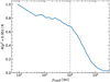 |
Fig. 16 Fraction of high confidence companions to the total number of identified companion candidates within a specified radius ρcutoff. We show the fractional amount of companions with pC > 0.95 to the total number N of preselected objects interior to our cutoff radius ρcutoff. The grey, dashed line marks the chosen cutoff radius of ρcutoff = 10 000 au. |
5.2 Quality assessment of derived Gaia properties
As we detected seven companion candidates in both SPHERE and Gaia measurements, these systems provide ideal test cases for assessing the quality of the companion properties that we derived for the remaining sample members. This analysis wasfocused on two important parameters that were extracted from our Gaia analysis as presented in Sect. 3, namely: (i) the co-movement hypothesis of the companion and (ii) the companion mass estimate.
For all these companion candidates (except the one detected for 2MASS J12560830-6926539) we derived a velocity ratio vproj∕vmax that is smaller than unity. This resulted in companionship probabilities pC > 0.95, indicating that these are gravitationally bound companions. These hypotheses are confirmed for all cases, when analyzing the relative astrometric offsets between the SPHERE and Gaia epochs as presented in Sect. 4. SPHERE and Gaia astrometric measurements are highly consistent and prove the claimed companionship status. Even though the astrometric measurements from both instruments do not agree within their uncertainties for the companion candidate around 2MASS J12560830-6926539, this is no indication that our classification scheme does not work. As detailed in Sect. 4.2.4, the primary is a visual binary itself that is unresolved in the Gaia catalog. For that reason, the measured astrometry is corrupted and does not agree with our SPHERE data. Previous works, however, have strongly indicated that the companion candidate is indeed gravitationally bound, and all three objects form a triple system.
We conclude that the differential velocities directly measured in the Gaia catalog are trustworthy, at least for companions that are as bright or brighter and at least as far in terms of their separation from the primary as the benchmark targets with complementary SPHERE data. Due to the small angular separation of less than 5′′.5, these are already quite challenging cases and for the majority of brighter and farther separated companions, a similar or better performance of the evaluation method can be expected. Further monitoring and reduction of the velocity uncertainties (as presented in Fig. 6) is required to confirm co-movement for all the companion candidates that were detected during our search. Precise measurements of the RVs of the companions are necessary to obtain a complete three dimensional picture of the orbital dynamics and parameters.
For all seven companions, the photometric masses determined by either SPHERE or Gaia are consistent within 2 σ intervals, especially with regard to the masses of the identified sub-stellar companions to TYC 8252-533-1, 2MASS J12560830-6926539, and 2MASS J13335481-6536414, which are in exceptional agreement. It is thus likely that the mass estimates we derived for all identified companions are good estimates for the actual object masses. Given its rather close separation to the primary star and a G band contrast of ΔG ≈ 6 mag, TYC 8252-533-1 B is one of the more challenging cases for extraction of Gaia photometry (which is also visualized by the proximity of the object to the red exclusion zone that is highlighted in Fig. 3). It is therefore likely that the extraction of these relevant Gaia parameters could be performed at higher accuracy, leading to more trustworthy results for the objects that are farther away from the red-dashed triangle in Fig. 4. Of course this is not true for companions that are closely located to Gaia’s G band magnitude limit of approximately 21 mag, for which the small amount of received flux creates larger uncertainties in the measured parameters.
When inspecting the derived masses for the potential triple system comprising two of our targets from the input catalog (2MASS J15241147-3030582 and 2MASS J15241303-3030572) and a third lower-mass companion, it appears that our mass estimates for the stellar members of this trio are quite different from the input masses we adopted from Pecaut & Mamajek (2016). As listed in Table C.1, we derived the same mass estimate of approximately 0.7 M⊙ for both stars, which should be very distinct with 1.1 M⊙ and 0.4 M⊙ for 2MASS J15241147-3030582 and 2MASS J15241303-3030572, respectively. This discrepancy is not caused by the marginally different parallaxes assumed for the corresponding primary, which only results in a magnitude difference of 0.05 mag. The main source of error stems from the two very different ages of 18 Myr and 1 Myr that Pecaut & Mamajek (2016) give for the two targets, which also results in the very different mass estimates of the third companion Gaia EDR3 6208136396122878976. Based on the same apparent G band magnitude of this object, we derived masses of 0.23 M⊙ and 0.08 M⊙, respectively,with the higher mass corresponding to the older system age. If the system is indeed a gravitationally bound stellar triple, which is strongly suggested by the derived values of pC ≈ 1, all three components should roughly be of the same age, which would also avoid the change in mass of more than 100% for the lightest member of the system. When trying to reproduce the stellar masses of the two targets from Pecaut & Mamajek (2016) based on the measured G band photometry and BT-Settl isochrones, we find best agreement with a system age of approximately 4 Myr, which provides masses of 1.13 M⊙, 0.45 M⊙, and 0.14 M⊙ for 2MASS J15241147-3030582, 2MASS J15241303-3030572, and Gaia EDR3 6208136396122878976, respectively.
We see similar age and mass discrepancies for the other multiple systems that contain stars from our input catalog as identified companion candidates. This clearly shows that our derived object masses have to be used carefully as they are heavily affected by the underlying system age. Further refinements of the stellar age such as updated Gaia distances and coevality constraints for the identified multiple systems are thus required to properly constrain derived objects masses. Further spectral coverage of the SEDs of the detected companions is also necessary, to determine their properties with much higher accuracy than our results, which are based on a single photometric data point. As most of the identified objects are reasonably separated from the primary,spectroscopic follow-up measurements are easily possible and can in most cases even be performed without any AO-assisted instruments.
Further data releases of the Gaia mission might also improve the parameters derived in this study, and it should be a straightforward exercise to update these results in the future. The photometric uncertainties, especially of the very faint objects, would certainly be improved with more observational data points, even though the provided G band magnitudes are already precise enough so that these have only had a marginal influence on the precision of the derived quantities. It is not clear if color measurements for all our companion candidates will be available in future releases, as most of these incompletely characterized objects are very close to a source of equal or higher brightness, which will always be problematic for precise photometric measurements. Astrometry at a higher level of accuracy will certainly help in rejecting or confirming marginal cases from our current study and will provide new candidate companions that were discarded by our present preselection, either due to non-existing proper motion measurements or overly large astrometric uncertainties.
5.3 Comparison to similar studies
There are two main studies that have utilized Gaia DR2 to reveal members of Sco-Cen. Goldman et al. (2018) identified additional Gaia members in the LCC, which is the Sco-Cen sub-group that YSES is focusing on. This moving group comprises several low-mass stellar and brown dwarf objects, whose membership had not been revealed before Gaia DR2. Damiani et al. (2019) have focused on the stellar population of Sco-Cen and they identified almost 11 000 pre-main-sequence members by Gaia astrometry and photometry. To assess whether any of our candidates have been picked up by either of these studies, we cross-matched our identified companions with the output catalogs of both surveys. We focused on the systems with a companionship probability of pC > 0.95 as presented in Table C.2 and we found that 20 of our detected companions were listed in both of the studied catalogs. One additional source was identified only by Goldman et al. (2018). Interestingly, only companions with a right ascension below 15h were picked up by either of these previous studies. This is not surprising with regard to the work of Goldman et al. (2018), as these authors were explicitly targeting the LCC, which does not extend to a right ascension greater than 15h. However, none of these discussed surveys identified individual binary or multiple systems as part of their analysis.
5.4 Completeness
We assessed the completeness of our companion detection method based on the completeness of the Gaia DR2 catalog. Using the selectionfunctions introduced by Boubert et al. (2020) and Boubert & Everall (2020), we derived the completeness as a function of the position on sky for objects down to the Gaia magnitude threshold of G = 21 mag. The resulting completeness map is presented in Fig. 17. The map shows clear patterns that correspond to the scanning scheme of the Gaia satellite. For most of the coordinates of our Sco-Centargets, the achieved completeness is higher than 80% and the LCC, which is covering an area of approximately 290° < l < 310° and − 10° < b < 20°, has a completeness coverage of almost 100%. As the underlying code is relying on Gaia DR2 we expect the actual completeness of Gaia EDR3 to be even higher.
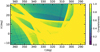 |
Fig. 17 Completeness of Gaia DR2 as a function of position on sky. The completeness is calculated for objects as faint as G = 21 mag. |
6 Conclusions
We present a method to find comoving companions utilizing the early version of the third data release of ESA’s Gaia mission. We applied this preselection algorithm to a sample of 480 K-type pre-main-sequence stars presented by Pecaut & Mamajek (2016) aiming to find new (sub-)stellar companions for them. With our selection criteria we identify 163 potential companions to 142 members of our input catalog, including 21 candidate triples systems. We could show that the sensitivity of Gaia to detect such companion candidates improves with increasing angular separation from the target star. For our K-type stars we reach the background limit of G ≈ 20 mag for separations larger than 10′′. Utilizing age estimates from Pecaut & Mamajek (2016), we converted the measured photometry to mass estimates of the companion candidates using BT-Settl (Allard et al. 2012; Baraffe et al. 2015) and MIST (Dotter 2016; Choi et al. 2016) models for (sub-)stellar objects. The age and distance of our sample allows for detections of objects with masses as low as 20 MJup.
To corroborate the companionship status of the preselected objects we performed tests based on the available photometry and relative astrometry. Our color-magnitude analysis, which was accessible for the majority of our candidate companions, is in agreement with evolutionary models of young, (sub-)stellar objects. We further compared differential projected velocities, vproj, of each potential binary to the maximum velocity that still permits bound orbits, vmax. Based on the posterior distributions of the calculated vproj to vmax ratios and the statistical constraints from the stellar density around the target star we derived likelihood estimates of a companion to be bound, pC. Only 27% from our identified companion candidates exhibited a companionship probability of less than 10%. Instead, 110 objects (67%) reside in the pC > 0.95 regime, which we designate as our high confidence targets henceforth. Amongst these we found ten candidate brown dwarf companions:
Gaia EDR3 5232514298301348864, M = 36.5 ± 2.4 MJup,
Gaia EDR3 6071087597497876480, M = 76.0 ± 16.7 MJup,
Gaia EDR3 5860803696599969280, M = 66.2 ± 4.5 MJup,
Gaia EDR3 6073106193460538240, M = 46.5 ± 3.3 MJup,
Gaia EDR3 6083750638540951552, M = 48.7 ± 11.1 MJup,
Gaia EDR3 6039427503765943040, M = 33.8 ± 3.6 MJup,
Gaia EDR3 5984404849554176256, M = 73.8 ± 4.4 MJup,
Gaia EDR3 6043486655875354112, M = 24.8 ± 1.0 MJup,
Gaia EDR3 6245781131640479360, M = 43.1 ± 5.8 MJup,
Gaia EDR3 6243833724749589760, M = 78.9 ± 12.5 MJup.
These ten brown dwarf companions are suitable for future follow-up observations with ground- and space-based telescopes, aiming to understand their atmospheric architectures and dynamical histories.
For seven of the detected candidate companions we used complementary high-contrast imaging data. These were collected with the SPHERE and NACO instruments as part of YSES, a direct imaging search for sub-stellar companions around Sun-like stars (Bohn et al. 2020a). The astrometry that was extracted from this near infrared data was in excellent agreement with the Gaia measurements and confirmed the companionship of six candidates. The remaining target, 2MASS J12560830-6926539, was resolved into a visual binary that was corrupting the astrometric measurements. This system is likely to be a triple with a brown dwarf companion of about 40 MJup.
Another interesting target that was observed with both instruments is TYC 8252-533-1. This solar-type star hosts a sub-stellar companion at a projected separation of 4′′.4 that was picked up by Gaia and could be directly imaged within the scope of our survey. Complementary data collected with SPHERE and NACO covered the spectral energy distribution of the companion from 1 to 4 microns and we derived an effective temperature of  , a surface gravity of
  dex, a radius of
  , and a luminosityof
  . We converted the latter parameter to an object mass by evaluation of BT-Settl isochrones at the system age of 5 ± 2 Myr, which provided a mass of
  . With a projected physical separation of 570 au, this brown dwarf companion is likely to reside beyond the debris disk that is found around its host star based on an infrared excess in WISE W3 and W4 bands. As postulated for the widely separated planetary-mass companion HD 106906 b, which was detected outside the circumstellar disk around its primary (Bailey et al. 2014), a star-like formation pathway for TYC 8252-533-1 B is favored over planetary formation channels, such as core accretion or gravitational instabilities in the protoplanetary disk.
The photometric mass estimates that were independently derived from SPHERE and Gaia data also agree very well for the seven targets that were observed with both instruments. We conclude that Gaia can properly characterize all objects from our sample that are at least equally bright and separated from their host stars. Nevertheless, we should treat the derived mass estimates for the remaining objects with some care, as these are based on a single photometric measurement; in addition, this parameter is very sensitive to the system age, which needs to be determined with greater accuracy in some cases.
In this work, we show that our proposed method is a viable tool for identifying comoving companions to Sco-Cen members based on Gaia data. It should be applicable to arbitrary samples of input stars, but some justified age and primary mass estimates are required to derive secondary masses and their companionship probability. The parameter space that is probed by this approach is highly complementary to the comparably small field of view of current high-contrast imaging instruments. To obtain a detailed understanding of the occurrence rates of giant, sub-stellar companions and their underlying formation mechanisms, it is important to include this population of widely separated objects.
Acknowledgements
We would like to thank the anonymous referee for the detailed feedback they provided. Their comments helped the authors to improve the quality of the manuscript. We dedicate this article to the memory of France Allard, who passed away in October 2020. Her groundbreaking work on low-mass stars, brown dwarfs, and exoplanets strongly shaped our current understanding of their atmospheric physics; the models she (co-)developed – that were also used in this work and that were frequently accessed by a vast number of researchers – will remain as a crucial foundation to all future studies in this field and astronomy in general. The research of A.J.B. leading to these results has received funding from the European Research Council under ERC Starting Grant agreement 678194 (FALCONER). Part of this research was carried out at the Jet Propulsion Laboratory, California Institute of Technology, under a contract with the National Aeronautics and Space Administration (80NM0018D0004). G.C. thanks the Swiss National Science Foundation for financial support under grant number 200021_169131. This research has used the SIMBAD database, operated at CDS, Strasbourg, France (Wenger et al. 2000). This work has used data from the European Space Agency (ESA) mission Gaia (https://www.cosmos.esa.int/gaia), processed by the Gaia Data Processing and Analysis Consortium (DPAC, https://www.cosmos.esa.int/web/gaia/dpac/consortium). Funding for the DPAC has been provided by national institutions, in particular the institutions participating in the Gaia Multilateral Agreement. This publication makes use of VOSA, developed under the Spanish Virtual Observatory project supported by the Spanish MINECO through grant AyA2017-84089. To achieve the scientific results presented in this article we made use of the Python programming language8, especially the SciPy (Virtanen et al. 2020), NumPy (Oliphant 2006), Matplotlib (Hunter 2007), emcee (Foreman-Mackey et al. 2013), scikit-image (Van der Walt et al. 2014), scikit-learn (Pedregosa et al. 2012), photutils (Bradley et al. 2016), and astropy (Astropy Collaboration 2013, 2018) packages.
Appendix A The input sample of K-type Sco-Cen members
As described in Sect. 3, some targets were excluded during our analysis from the full list of K-type Sco-Cen members as presented byPecaut & Mamajek (2016). These stars and the reasons for their exclusions are listed in Table A.1.
We further found that some targets of the input sample were identified as companion candidates during our preselection. These duplications are presented in Table A.2.
Targets excluded from our analysis.
Duplications amongst our list of preselected candidate companions.
Appendix B High-contrast imaging observations
We present the setup of our SPHERE and NACO observations and the atmospheric conditions during the data acquisition in Table B.1. The final images of our SPHERE and NACO data reductions on TYC 8252-533-1 are presented in Fig. B.1. In Fig. B.2, we show the remaining stellar companions to YSES targets as observed with SPHERE.
High-contrast imaging observations of YSES targets.
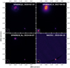 |
Fig. B.1 Reduced SPHERE and NACO data of TYC 8252-533-1 and its brown dwarf companion. For each of the presented filters we show the median of the full observing sequence. The images are derotated such that north points up and east towards the left. No PSF subtraction is applied for the SPHERE data – the star’s intensity is attenuated by a coronagraphic mask, and it is located at the origin of the coordinate system that is representing the differential offsets in RA and Dec. No coronagraph was used for the NACO observing sequence and the stellar PSF is removed by classical ADI (Marois et al. 2006) to obtain the presented image; we did not perform any PSF subtraction for the extraction of the companion’s photometry and astrometry. The companion is detected at a separation of ~ 4′′.4 in south-western direction from the primary. In the lower-left section of each panel, we present the non-coronagraphic stellar PSF as a reference. The images are shown with an arbitrary logarithmic color scale. |
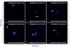 |
Fig. B.2 (Sub)stellar companions identified in SPHERE data. We present the derotated and median combined coronagraphic images for the epochs and filters as indicated in the upper right of each panel. The star is located behind the coronagraphic mask at the center of each panel. The companions that were also identified by our Gaia selection algorithm are highlighted by the white arrows. As discussed in Sect. 4.2.4, there is an additional, very close companion to 2MASS J12560830-6926539. With a separation of merely 0′′.2 this stellar companion is not identified by our Gaia selection method. In the lower-left section of each panel, we present the non-coronagraphic flux PSFs of each target. In all frames north points up and east towards the left. |
Appendix C Identified companions
We present all identified candidate companions in Table C.1.
The list of high-confidence companions is presented in Table C.2
Identifiers and properties of all identified candidate companions to K type Sco-Cen members from Pecaut & Mamajek (2016).
Gaia companion candidates with pC > 0.95 that were identified to K-type Sco-Cen members. In the last column we report whether these systems have been mentioned in previous literature. A full version of the table that is including the parameter uncertainties is available online.
Appendix D Posterior distribution of the MCMC analysis
In Fig. D.1, we present the posterior distribution of our MCMC-based SED fitting of TYC 8252-533-1 B. After discarding the burn-in phase and thinning the chains, the visualized 45,000 posterior samples remained. We additionally present the luminosities that are derived from the input parameters (Teff,  , R) as these quantities are used for the determination of the object’s mass. We derived
 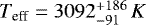 ,
, 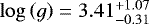 dex,
dex, 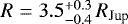 , and
, and  as the 95% quantiles around the medians of the distributions.
 |
Fig. D.1 Posterior distribution of the MCMC-based fit to the SED of TYC 8252-533-1 B. The blue, dashed lines represent the 2.5th, 50th, and 97.5th percentiles of the marginalized distributions. |
References
- Alcalá, J. M., Natta, A., Manara, C. F., et al. 2014, A&A, 561, A2 [NASA ADS] [CrossRef] [EDP Sciences] [Google Scholar]
- Alcalá, J. M., Manara, C. F., Natta, A., et al. 2017, A&A, 600, A20 [NASA ADS] [CrossRef] [EDP Sciences] [Google Scholar]
- Alibert, Y., Mordasini, C., Benz, W., & Winisdoerffer, C. 2005, A&A, 434, 343 [NASA ADS] [CrossRef] [EDP Sciences] [Google Scholar]
- Allard, F., Homeier, D., & Freytag, B. 2012, Philos. Trans. Roy. Soc. Lond. A, 370, 2765 [NASA ADS] [Google Scholar]
- Astropy Collaboration (Robitaille, T. P., et al.) 2013, A&A, 558, A33 [NASA ADS] [CrossRef] [EDP Sciences] [Google Scholar]
- Astropy Collaboration (Price-Whelan, A. M., et al.) 2018, AJ, 156, 123 [Google Scholar]
- Backman, D. E., & Paresce, F. 1993, in Protostars and Planets III, eds. E. H. Levy, & J. I. Lunine, 1253 [Google Scholar]
- Bailer-Jones, C. A. L., Rybizki, J., Fouesneau, M., Demleitner, M., & Andrae, R. 2021, AJ, 161, 147 [Google Scholar]
- Bailey, V., Meshkat, T., Reiter, M., et al. 2014, ApJ, 780, L4 [Google Scholar]
- Baraffe, I., Homeier, D., Allard, F., & Chabrier, G. 2015, A&A, 577, A42 [NASA ADS] [CrossRef] [EDP Sciences] [Google Scholar]
- Bayo, A., Rodrigo, C., Barrado Y Navascués, D., et al. 2008, A&A, 492, 277 [NASA ADS] [CrossRef] [EDP Sciences] [Google Scholar]
- Beuzit, J. L., Vigan, A., Mouillet, D., et al. 2019, A&A, 631, A155 [NASA ADS] [CrossRef] [EDP Sciences] [Google Scholar]
- Bohn, A. J., Kenworthy, M. A., Ginski, C., et al. 2019, A&A, 624, A87 [EDP Sciences] [Google Scholar]
- Bohn, A. J., Kenworthy, M. A., Ginski, C., et al. 2020a, MNRAS, 492, 431 [Google Scholar]
- Bohn, A. J., Kenworthy, M. A., Ginski, C., et al. 2020b, ApJ, 898, L16 [Google Scholar]
- Bohn, A. J., Southworth, J., Ginski, C., et al. 2020c, A&A, 635, A73 [NASA ADS] [CrossRef] [EDP Sciences] [Google Scholar]
- Bohn, A. J., Ginski, C., Kenworthy, M. A., et al. 2021, A&A, 648, A73 [NASA ADS] [CrossRef] [EDP Sciences] [Google Scholar]
- Bonavita, M., Gratton, R., Desidera, S., et al. 2021, ArXiv e-prints, [arXiv:2103.13706] [Google Scholar]
- Boss, A. P. 1997, Science, 276, 1836 [Google Scholar]
- Boss, A. P. 2011, ApJ, 731, 74 [Google Scholar]
- Boubert, D., & Everall, A. 2020, MNRAS, 497, 4246 [NASA ADS] [CrossRef] [Google Scholar]
- Boubert, D., Everall, A., & Holl, B. 2020, MNRAS, 497, 1826 [NASA ADS] [CrossRef] [Google Scholar]
- Bradley, L., Sipocz, B., Robitaille, T., et al. 2016, Photutils: Photometry Tools [Google Scholar]
- Chabrier, G. 2003, PASP, 115, 763 [Google Scholar]
- Chabrier, G., Baraffe, I., Leconte, J., Gallardo, J., & Barman, T. 2009, in AIP Conf. Ser., 1094, 15th Cambridge Workshop on Cool Stars, Stellar Systems, and the Sun, ed. E. Stempels, 102 [Google Scholar]
- Chauvin, G., Desidera, S., Lagrange, A. M., et al. 2017, A&A, 605, L9 [NASA ADS] [CrossRef] [EDP Sciences] [Google Scholar]
- Choi, J., Dotter, A., Conroy, C., et al. 2016, ApJ, 823, 102 [Google Scholar]
- Comerón, F. 2008, The Lupus Clouds, 5, eds. B. Reipurth, 295 [Google Scholar]
- Cropper, M., Katz, D., Sartoretti, P., et al. 2018, A&A, 616, A5 [NASA ADS] [CrossRef] [EDP Sciences] [Google Scholar]
- Cutri, R. M., Skrutskie, M. F., van Dyk, S., et al. 2003, VizieR Online Data Catalog: II/246 [Google Scholar]
- Cutri, R. M., Skrutskie, M. F., van Dyk, S., et al. 2012a, VizieR Online Data Catalog: II/281 [Google Scholar]
- Cutri, R. M. et al. 2012b, VizieR Online Data Catalog: II/311 [Google Scholar]
- Damiani, F., Prisinzano, L., Pillitteri, I., Micela, G., & Sciortino, S. 2019, A&A, 623, A112 [NASA ADS] [CrossRef] [EDP Sciences] [Google Scholar]
- DENIS Consortium. 2005, VizieR Online Data Catalog: II/263 [Google Scholar]
- de Zeeuw, P. T., Hoogerwerf, R., de Bruijne, J. H. J., Brown, A. G. A., & Blaauw, A. 1999, AJ, 117, 354 [Google Scholar]
- Dodson-Robinson, S. E., Veras, D., Ford, E. B., & Beichman, C. A. 2009, ApJ, 707, 79 [Google Scholar]
- Dotter, A. 2016, ApJS, 222, 8 [Google Scholar]
- Duchêne, G.,& Kraus, A. 2013, ARA&A, 51, 269 [CrossRef] [Google Scholar]
- Duquennoy, A., & Mayor, M. 1991, A&A, 500, 337 [NASA ADS] [Google Scholar]
- Durisen, R. H., Boss, A. P., Mayer, L., et al. 2007, in Protostars and Planets V, eds. B. Reipurth, D. Jewitt, & K. Keil, 607 [Google Scholar]
- Eggleton, P. P., & Tokovinin, A. A. 2008, MNRAS, 389, 869 [Google Scholar]
- El-Badry, K., Rix, H.-W., & Heintz, T. M. 2021, MNRAS, 506, 2269 [NASA ADS] [CrossRef] [Google Scholar]
- Elliott, P., Huélamo, N., Bouy, H., et al. 2015, A&A, 580, A88 [NASA ADS] [CrossRef] [EDP Sciences] [Google Scholar]
- Fontanive, C., Rice, K., Bonavita, M., et al. 2019, MNRAS, 485, 4967 [Google Scholar]
- Fontanive, C., & Bardalez Gagliuffi, D. 2021, Front. Astron. Space Sci., 8, 16 [NASA ADS] [CrossRef] [Google Scholar]
- Foreman-Mackey, D., Hogg, D. W., Lang, D., & Goodman, J. 2013, PASP, 125, 306 [Google Scholar]
- Gaia Collaboration (Prusti, T., et al.) 2016, A&A, 595, A1 [NASA ADS] [CrossRef] [EDP Sciences] [Google Scholar]
- Gaia Collaboration (Brown, A. G. A., et al.) 2018, A&A, 616, A1 [NASA ADS] [CrossRef] [EDP Sciences] [Google Scholar]
- Gaia Collaboration (Brown, A. G. A., et al.) 2021, A&A, 649, A1 [NASA ADS] [CrossRef] [EDP Sciences] [Google Scholar]
- Goldman, B., Röser, S., Schilbach, E., Moór, A. C., & Henning, T. 2018, ApJ, 868, 32 [Google Scholar]
- Haffert, S. Y., Bohn, A. J., de Boer, J., et al. 2019, Nat. Astron., 3, 749 [Google Scholar]
- Henden, A. A., Levine, S. E., Terrell, D., Smith, T. C., & Welch, D. 2012, J. Am. Assoc. Variable Star Observers (JAAVSO), 40, 430 [NASA ADS] [Google Scholar]
- Høg, E., Fabricius, C., Makarov, V. V., et al. 2000, A&A, 355, L27 [Google Scholar]
- Hunter, J. D. 2007, Comput. Sci. Eng., 9, 90 [NASA ADS] [CrossRef] [Google Scholar]
- Janson, M., Hormuth, F., Bergfors, C., et al. 2012, ApJ, 754, 44 [Google Scholar]
- Keppler, M., Benisty, M., Müller, A., et al. 2018, A&A, 617, A44 [NASA ADS] [CrossRef] [EDP Sciences] [Google Scholar]
- Konopacky, Q. M., Rameau, J., Duchêne, G., et al. 2016, ApJ, 829, L4 [Google Scholar]
- Kouwenhoven, M. B. N., Goodwin, S. P., Parker, R. J., et al. 2010, MNRAS, 404, 1835 [NASA ADS] [Google Scholar]
- Kratter, K. M., Murray-Clay, R. A., & Youdin, A. N. 2010, ApJ, 710, 1375 [Google Scholar]
- Kraus, A. L., & Hillenbrand, L. A. 2008, ApJ, 686, L111 [Google Scholar]
- Kroupa, P. 2001, MNRAS, 322, 231 [NASA ADS] [CrossRef] [Google Scholar]
- Lagrange, A. M., Gratadour, D., Chauvin, G., et al. 2009, A&A, 493, L21 [NASA ADS] [CrossRef] [EDP Sciences] [Google Scholar]
- Lagrange, A. M., Bonnefoy, M., Chauvin, G., et al. 2010, Science, 329, 57 [Google Scholar]
- Lallement, R., Vergely, J. L., Valette, B., et al. 2014, A&A, 561, A91 [NASA ADS] [CrossRef] [EDP Sciences] [Google Scholar]
- Lambrechts, M., & Johansen, A. 2012, A&A, 544, A32 [NASA ADS] [CrossRef] [EDP Sciences] [Google Scholar]
- Launhardt, R., Henning, T., Quirrenbach, A., et al. 2020, A&A, 635, A162 [NASA ADS] [CrossRef] [EDP Sciences] [Google Scholar]
- Lenzen, R., Hartung, M., Brandner, W., et al. 2003, in Society of Photo-Optical Instrumentation Engineers (SPIE) Conference Series, 4841, Instrument Design and Performance for Optical/Infrared Ground-based Telescopes, eds. M. Iye, & A. F. M. Moorwood, 944 [Google Scholar]
- Lindegren, L., Bastian, U., Biermann, M., et al. 2021a, A&A, 649, A4 [EDP Sciences] [Google Scholar]
- Lindegren, L., Klioner, S. A., Hernández, J., et al. 2021b, A&A, 649, A2 [EDP Sciences] [Google Scholar]
- Macintosh, B., Graham, J. R., Ingraham, P., et al. 2014, Proc. Natl. Acad. Sci. U.S.A., 111, 12661 [Google Scholar]
- Macintosh, B., Graham, J. R., Barman, T., et al. 2015, Science, 350, 64 [Google Scholar]
- Maire, A.-L., Langlois, M., Dohlen, K., et al. 2016, in Ground-based and Airborne Instrumentation for Astronomy VI, 9908, 990834 [Google Scholar]
- Malmberg, D., Davies, M. B., & Heggie, D. C. 2011, MNRAS, 411, 859 [Google Scholar]
- Marois, C., Lafrenière, D., Doyon, R., Macintosh, B., & Nadeau, D. 2006, ApJ, 641, 556 [Google Scholar]
- Marois, C., Macintosh, B., Barman, T., et al. 2008, Science, 322, 1348 [Google Scholar]
- Marois, C., Zuckerman, B., Konopacky, Q. M., Macintosh, B., & Barman, T. 2010, Nature, 468, 1080 [NASA ADS] [CrossRef] [Google Scholar]
- Mawet, D., David, T., Bottom, M., et al. 2015, ApJ, 811, 103 [NASA ADS] [CrossRef] [Google Scholar]
- Mayor, M., & Mazeh, T. 1987, A&A, 171, 157 [NASA ADS] [Google Scholar]
- Milli, J., Hibon, P., Christiaens, V., et al. 2017, A&A, 597, L2 [NASA ADS] [CrossRef] [EDP Sciences] [Google Scholar]
- Moór, A., Pascucci, I., Kóspál, Á., et al. 2011, ApJS, 193, 4 [CrossRef] [Google Scholar]
- Oliphant, T. E. 2006, A guide to NumPy (Trelgol Publishing USA) [Google Scholar]
- Pawellek, N., Krivov, A. V., Marshall, J. P., et al. 2014, ApJ, 792, 65 [Google Scholar]
- Pecaut, M. J.,& Mamajek, E. E. 2016, MNRAS, 461, 794 [NASA ADS] [CrossRef] [Google Scholar]
- Pedregosa, F., Varoquaux, G., Gramfort, A., et al. 2012, ArXiv e-prints, [arXiv:1201.0490] [Google Scholar]
- Pollack, J. B., Hubickyj, O., Bodenheimer, P., et al. 1996, Icarus, 124, 62 [NASA ADS] [CrossRef] [Google Scholar]
- Rafikov, R. R. 2005, ApJ, 621, L69 [Google Scholar]
- Raghavan, D., McAlister, H. A., Henry, T. J., et al. 2010, ApJS, 190, 1 [Google Scholar]
- Rameau, J., Chauvin, G., Lagrange, A. M., et al. 2013, ApJ, 772, L15 [Google Scholar]
- Raymond, S. N., Armitage, P. J., Moro-Martín, A., et al. 2012, A&A, 541, A11 [NASA ADS] [CrossRef] [EDP Sciences] [Google Scholar]
- Riaz, B., Gizis, J. E., & Harvin, J. 2006, AJ, 132, 866 [Google Scholar]
- Riello, M., De Angeli, F., Evans, D. W., et al. 2021, A&A, 649, A3 [NASA ADS] [CrossRef] [EDP Sciences] [Google Scholar]
- Rousset, G., Lacombe, F., Puget, P., et al. 2003, in Society of Photo-Optical Instrumentation Engineers (SPIE) Conference Series, 4839, Adaptive Optical System Technologies II, eds. P. L. Wizinowich, & D. Bonaccini, 140 [Google Scholar]
- Schmidt, T. O. B., Neuhäuser, R., Seifahrt, A., et al. 2008, A&A, 491, 311 [NASA ADS] [CrossRef] [EDP Sciences] [Google Scholar]
- Skrutskie, M. F., Cutri, R. M., Stiening, R., et al. 2006, AJ, 131, 1163 [NASA ADS] [CrossRef] [Google Scholar]
- Stolker, T., Bonse, M. J., Quanz, S. P., et al. 2019, A&A, 621, A59 [NASA ADS] [CrossRef] [EDP Sciences] [Google Scholar]
- Stolker, T., Marleau, G. D., Cugno, G., et al. 2020, A&A, 644, A13 [EDP Sciences] [Google Scholar]
- Tokovinin, A., Mason, B. D., & Hartkopf, W. I. 2010, AJ, 139, 743 [NASA ADS] [CrossRef] [Google Scholar]
- Tokovinin, A., Mason, B. D., Mendez, R. A., Horch, E. P., & Briceño, C. 2019, AJ, 158, 48 [NASA ADS] [CrossRef] [Google Scholar]
- Torres, C. A. O., Quast, G. R., da Silva, L., et al. 2006, A&A, 460, 695 [NASA ADS] [CrossRef] [EDP Sciences] [Google Scholar]
- Van der Walt, S., Schönberger, J. L., Nunez-Iglesias, J., et al. 2014, PeerJ, 2, e453 [Google Scholar]
- Virtanen, P., Gommers, R., Oliphant, T. E., et al. 2020, Nat. Methods, 17, 261 [Google Scholar]
- Wang, J., Fischer, D. A., Horch, E. P., & Xie, J.-W. 2015, ApJ, 806, 248 [NASA ADS] [CrossRef] [Google Scholar]
- Wenger, M., Ochsenbein, F., Egret, D., et al. 2000, A&AS, 143, 9 [NASA ADS] [CrossRef] [EDP Sciences] [Google Scholar]
- Zhang, Z., Liu, M. C., Hermes, J. J., et al. 2020, ApJ, 891, 171 [CrossRef] [Google Scholar]
- Zhang, Z., Liu, M. C., Claytor, Z. R., et al. 2021, ApJ, 916, L11 [NASA ADS] [CrossRef] [Google Scholar]
Compiled from Table 7 of Pecaut & Mamajek (2016).
The applied correction formula for the parallactic zero point bias is available at https://gitlab.com/icc-ub/public/gaiadr3_zeropoint
The applied correction formula for the G band magnitudes is available at https://github.com/agabrown/gaiaedr3-6p-gband-correction
To report the full output of our algorithm, we did not remove these duplications from the table presented in Appendix C. All further analysis, however, is performed on the cleaned sample of 163 individual companion candidates.
We note that these age estimates rely on pre-Gaia parallaxes that were derived kinematically and which might differ from the value reported in Gaia EDR3. A reassessment of these parameters – especially for the identified systems with low-mass companions – is advisable, but beyond the scope of this work.
This statement is verified by the lowest magnitude contrast ΔMag between primary and secondary that is measured in the L′ band (see Table 5).
Python Software Foundation, https://www.python.org/
All Tables
SPHERE astrometric and photometric measurements of stellar companions identified by the Gaia search.
Identifiers and properties of all identified candidate companions to K type Sco-Cen members from Pecaut & Mamajek (2016).
Gaia companion candidates with pC > 0.95 that were identified to K-type Sco-Cen members. In the last column we report whether these systems have been mentioned in previous literature. A full version of the table that is including the parameter uncertainties is available online.
All Figures
|
Fig. 1 Input sample of K-type pre-main-sequence stars in Sco-Cen. We show the sky positions of the targets in galactic coordinates and the color of the markers indicates the distance to the objects. Members of the YSES subsample are highlighted by the black outlines around the markers. The star highlights TYC 8252-533-1, whose brown dwarf companion is analyzed in Sect. 4.1. |
| In the text | |
|
Fig. 2 Astrometric and photometric properties of the input sample along with the preselected list of candidate companions (CCs). In the top panel, we present the distributions of the object parallaxes, proper motions, and magnitudes from both samples. In the lower panel, the uncertainties are shown. The colored values in the upper right of each panel indicate the median and the 68% confidence intervals of the associated distributions. |
| In the text | |
|
Fig. 3 Identified companion candidates to K-type Sco-Cen members. Members of the YSES subsample are highlighted by the black outline around the marker. The orange star highlights the brown dwarf companion TYC 8252-533-1 B that is analyzed in Sect. 4.1. The apparent Gaia G band magnitude is presented as a function of projected separation in arcseconds. Due to the PSF halo of the primary, the detectable magnitude threshold increases with larger separations from the host. This area of reduced sensitivity is indicated by the red, dashed triangle. The gray-shaded region represents the field of view of the SPHERE/IRDIS detector. |
| In the text | |
|
Fig. 4 Identified companion candidates to K-type Sco-Cen members II. Members of the YSES subsample are highlighted by the blackoutline around the marker. The orange star highlights TYC 8252-533-1 B analyzed in Sect. 4.1. The companion mass is presented as a function of projected separation in Astronomical Units. Mass conversion was performed by comparison to BT-Settl and MIST models evaluated at the system age. The dashed red line at 80 MJup indicates the threshold between brown dwarfs and stellar mass companions. |
| In the text | |
|
Fig. 5 Color-magnitude diagram of identified companion candidates to K-type stars in Sco-Cen. The colors of the markers indicate the projected separation between host and companion. The orange line represents a combination of MIST and BT-Settl isochrones for an age of 15 Myr. |
| In the text | |
|
Fig. 6 Relative velocities of identified companions of a sample of K-type Sco-Cen members. We show the ratio of the differential projected velocities vproj to the maximum velocity that allows a gravitationally bound system vmax as defined in Eq. (6). This parameter is a measure of whether our preselected candidate companions are part of a binary system; a value greater than unity renders this scenario as unlikely. These two different regimes are separated by the dashed red line. The colors of the markers indicate the mass of the corresponding candidate companion. To focus primarily on the sub-stellar objects in our sample the color bar is cut off at masses that are higher than 100 MJup. Markers with a black outline refer to members of the YSES subsample and TYC 8252-533-1 B is highlighted by the star. |
| In the text | |
|
Fig. 7 Properties of high-confidence companions to K type Sco-Cen members. Left panel: distribution of separations amongst our high confidence sample. Right panel: mass distribution among this sample. The red dashed line indicates the threshold of brown dwarf and stellar-mass companions at 80 MJup. |
| In the text | |
|
Fig. 8 Proper motion analysis of TYC 8252-533-1 B. The colored markers represent the relative offsets in RA and Dec with respect to the primary that we measured in SPHERE and NACO imaging data or derived from the Gaia DR2 and EDR3 catalogs. The blue dashed line illustrates the trajectory of a static background object at infinity and the white markers along the curve represent the hypothetical positions of such an object at the epoch of the corresponding observation. |
| In the text | |
|
Fig. 9 SED of TYC 8252-533-1 B. The yellow, orange, and red squares indicate the photometry we measured for Gaia, SPHERE, and NACO filters, respectively. The bars in the x direction indicate the width of the filter transmission curves. The blue curve presents the median model from our posterior distribution of the SED fit as shown in Fig. D.1. We present the integrated flux of this median model in the applied filters with the grey squares and we visualize 100 randomly selected models from our posterior distribution as grey curves. In the bottom panel, we present the residuals of the fit. |
| In the text | |
|
Fig. 10 Proper motion analysis of 2MASS J12195938-5018404 B. See Fig. 8 for a detailed description of the plot elements. |
| In the text | |
|
Fig. 11 Proper motion analysis of 2MASS J12391404-5454469 B. See Fig. 8 for a detailed description of the plot elements. |
| In the text | |
|
Fig. 12 Proper motion analysis of 2MASS J12505143-5156353 B. See Fig. 8 for a detailed description of the plot elements. |
| In the text | |
|
Fig. 13 Proper motion analysis of 2MASS J12560830-6926539 B. See Fig. 8 for a detailed description of the plot elements. |
| In the text | |
|
Fig. 14 Proper motion analysis of 2MASS J13130714-4537438 B. See Fig. 8 for a detailed description of the plot elements. |
| In the text | |
|
Fig. 15 Proper motion analysis of 2MASS J13335481-6536414 B. See Fig. 8 for a detailed description of the plot elements. |
| In the text | |
|
Fig. 16 Fraction of high confidence companions to the total number of identified companion candidates within a specified radius ρcutoff. We show the fractional amount of companions with pC > 0.95 to the total number N of preselected objects interior to our cutoff radius ρcutoff. The grey, dashed line marks the chosen cutoff radius of ρcutoff = 10 000 au. |
| In the text | |
|
Fig. 17 Completeness of Gaia DR2 as a function of position on sky. The completeness is calculated for objects as faint as G = 21 mag. |
| In the text | |
|
Fig. B.1 Reduced SPHERE and NACO data of TYC 8252-533-1 and its brown dwarf companion. For each of the presented filters we show the median of the full observing sequence. The images are derotated such that north points up and east towards the left. No PSF subtraction is applied for the SPHERE data – the star’s intensity is attenuated by a coronagraphic mask, and it is located at the origin of the coordinate system that is representing the differential offsets in RA and Dec. No coronagraph was used for the NACO observing sequence and the stellar PSF is removed by classical ADI (Marois et al. 2006) to obtain the presented image; we did not perform any PSF subtraction for the extraction of the companion’s photometry and astrometry. The companion is detected at a separation of ~ 4′′.4 in south-western direction from the primary. In the lower-left section of each panel, we present the non-coronagraphic stellar PSF as a reference. The images are shown with an arbitrary logarithmic color scale. |
| In the text | |
|
Fig. B.2 (Sub)stellar companions identified in SPHERE data. We present the derotated and median combined coronagraphic images for the epochs and filters as indicated in the upper right of each panel. The star is located behind the coronagraphic mask at the center of each panel. The companions that were also identified by our Gaia selection algorithm are highlighted by the white arrows. As discussed in Sect. 4.2.4, there is an additional, very close companion to 2MASS J12560830-6926539. With a separation of merely 0′′.2 this stellar companion is not identified by our Gaia selection method. In the lower-left section of each panel, we present the non-coronagraphic flux PSFs of each target. In all frames north points up and east towards the left. |
| In the text | |
|
Fig. D.1 Posterior distribution of the MCMC-based fit to the SED of TYC 8252-533-1 B. The blue, dashed lines represent the 2.5th, 50th, and 97.5th percentiles of the marginalized distributions. |
| In the text | |
Current usage metrics show cumulative count of Article Views (full-text article views including HTML views, PDF and ePub downloads, according to the available data) and Abstracts Views on Vision4Press platform.
Data correspond to usage on the plateform after 2015. The current usage metrics is available 48-96 hours after online publication and is updated daily on week days.
Initial download of the metrics may take a while.