| Issue |
A&A
Volume 656, December 2021
|
|
|---|---|---|
| Article Number | A76 | |
| Number of page(s) | 9 | |
| Section | Planets and planetary systems | |
| DOI | https://doi.org/10.1051/0004-6361/202141502 | |
| Published online | 03 December 2021 | |
The 12CO/13CO isotopologue ratio of a young, isolated brown dwarf
Possibly distinct formation pathways of super-Jupiters and brown dwarfs
1
Leiden Observatory, Leiden University,
Postbus 9513,
2300 RA,
Leiden, The Netherlands
e-mail: This email address is being protected from spambots. You need JavaScript enabled to view it.
2
Max-Planck-Institut für Astronomie,
Königstuhl 17,
69117
Heidelberg, Germany
Received:
9
June
2021
Accepted:
21
September
2021
Abstract
Context. Linking atmospheric characteristics of planets to their formation pathways is a central theme in the study of extrasolar planets. Although the 12C/13C isotope ratio shows little variation in the Solar System, the atmosphere of a super-Jupiter was recently shown to be rich in 13CO, possibly as a result of dominant ice accretion beyond the CO snow line during its formation. Carbon isotope ratios are therefore suggested to be a potential tracer of formation pathways of planets.
Aims. In this work, we aim to measure the 12CO/13CO isotopologue ratio of a young, isolated brown dwarf. While the general atmospheric characteristics of young, low-mass brown dwarfs are expected to be very similar to those of super-Jupiters, their formation pathways may be different, leading to distinct isotopologue ratios. In addition, such objects allow high-dispersion spectroscopy at high signal-to-noise ratios.
Methods. We analysed archival K-band spectra of the L dwarf 2MASS J03552337+1133437 taken with NIRSPEC at the Keck telescope. A free retrieval analysis was applied to the data using the radiative transfer code petitRADTRANS coupled with the nested sampling tool PyMultiNest to determine the isotopologue ratio 12CO/13CO in its atmosphere.
Results. The isotopologue 13CO is detected in the atmosphere through the cross-correlation method at a signal-to-noise of ~8.4. The detection significance is determined to be ~9.5σ using a Bayesian model comparison between two retrieval models (including or excluding 13CO). We retrieve an isotopologue 12CO/13CO ratio of 97−18+25 (90% uncertainty), marginally higher than the local interstellar standard. Its C/O ratio of ~0.56 is consistent with the solar value.
Conclusions. Although only one super-Jupiter and one brown dwarf now have a measured 12CO/13CO ratio, it is intriguing that they are different, possibly hinting to distinct formation pathways. Regardless of spectroscopic similarities, isolated brown dwarfs may experience a top-down formation via gravitational collapse, which resembles star formation, while giant exoplanets favourably form through core accretion, which potentially alters isotopologue ratios in their atmospheres depending on the material they accrete from protoplanetary disks. This further emphasises atmospheric carbon isotopologue ratio as a tracer of the formation history of exoplanets. In the future, analyses such as those presented here should be conducted on a wide range of exoplanets using medium-to-high-resolution spectroscopy to further assess planet formation processes.
Key words: brown dwarfs / planets and satellites: atmospheres
© ESO 2021
1 Introduction
Planet formation and evolution are expected to leave imprints on the observed spectra of exoplanets. In bridging the gap between the spectral characterisation and formation mechanisms, isotopologue ratios have been suggested as informative tracers of planet formation conditions and evolutionary history (Clayton & Nittler 2004; Zhang et al. 2021). In the Solar System, deuterium/hydrogen (D/H) ratios demonstrate significant variations across planets, comets, and meteorites (Altwegg et al. 2015). While the D/H ratios in Jupiter and Saturn are consistent with the protosolar value, Uranus and Neptune are found to be enhanced in deuterium (Feuchtgruber et al. 2013), which is attributed to a likely increased contribution from accretion of D-rich ices beyond the water snow line. The terrestrial planets Earth, Mars, and Venus have higher D/H ratios (Drake 2005), indicating not only solid accretion, but also atmospheric loss. Therefore, isotope ratios in planetary atmospheres can reflect the material reservoir of the birth environment, the formation mechanism (via core accretion or gravitational collapse), the relative importance of gas or ice accretion, and the atmospheric evolution.
In contrast with D/H ratios, carbon isotope ratios are found to be roughly constant in the Solar System (Woods 2009), and therefore they are less effective diagnostic tools. However, the recent measurement of the 12CO/13CO isotopologue abundance ratio in an exoplanet may require a reassessment of its diagnostic value. The 13CO isotopologue was detected at a significance of 6σ in the atmosphere of the super-Jupiter TYC 8998 b. Intriguingly, the atmosphere is reported to be 13CO -rich with a 12CO/13CO abundance ratio of 31, which is significantly lower than the local interstellar standard at ~68 (Zhang et al. 2021). A formation outside the CO snow line with a large contribution from ice-accretion (as an analogy to the D-enrichment in Solar System planets) has been invoked to explain the enrichment. Since the Solar System planets are thought to be formed within the CO snow line, no substantial enrichment in 13C is expected, because the bulk of their carbon reservoirs originate from CO gas in the inner disk, where 13C is not enhanced. It therefore suggests that the atmospheric carbon isotopologue ratios could also shed light on the formation history of exoplanets, especially for the directly imaged populations, which are observed at wide orbits beyond the CO snow line.
Several carbon fractionation processes in molecular clouds, young stellar objects (YSOs), and protoplanetary disks are suggested toalter the CO isotopologue ratios in the birth environment of planets, including isotopic ion exchange reactions (Langer et al. 1984; Milam et al. 2005), isotope-selective photodissociation (Bally & Langer 1982; van Dishoeck & Black 1988; Visser et al. 2009; Miotello et al. 2014), and gas-to-ice isotopologue partitioning (Acharyya et al. 2007; Smith et al. 2015). Depending on the location of the proto-planets and the material (gas or ice) they accrete from the environment, the isotopologueratios in the atmospheres may deviate from the ISM standard. Therefore, detailed modelling of carbon fractionation in protoplanetary disks coupled with planet formation models have the potential to locate the birthplace and identify the formation mechanism of planets, like suggested for carbon-to-oxygen (C/O) ratios (Öberg et al. 2011; Madhusudhan et al. 2014; Mordasini et al. 2016; Cridland et al. 2020). Moreover, combining evidence from different observables, such as 12C/13C, D/H, and C/O ratios, allows for a more comprehensive understanding of the formation process.
Compared to the D/H ratios (~10−5) which can potentially be probed via HDO/H2O and CH3D/CH4 (Morley et al. 2019; Mollière & Snellen 2019), the 12C/13C ratios (≲100) are more readily detectable and attained from the ground with high-resolution spectroscopy targeting 12CO /13CO (Mollière & Snellen 2019). In addition to the recent result for a super-Jupiter, carbon isotopologue ratios have been measured toward various sources beyond the Solar System, including the interstellar medium (ISM) (Langer & Penzias 1993; Milam et al. 2005; Yan et al. 2019), YSOs and protostars in gas and ices (Boogert et al. 2000, 2002; Pontoppidan et al. 2005; Jørgensen et al. 2016, 2018; Smith et al. 2015), giant stars, solar-type stars, and M dwarfs (Sneden et al. 1986; Botelho et al. 2020; Tsuji 2016; Crossfield et al. 2019), but not yet towards brown dwarfs. In this paper, we carry out a similar analysis to Zhang et al. (2021) on archival high-resolution Keck/NIRSPEC data of a young, isolated brown dwarf. While its general atmospheric characteristics are expected to be very similar to those of super-Jupiters, its formation pathways may be different, leading to distinct isotopologue ratios. In addition, its spectrum can be studied at high signal-to-noise, and hence is more accessible.
We present the observations and spectrum extraction in Sect. 2, followed by a description of the retrieval model in Sect. 3. The retrieval results and the measurement of CO isotopologue ratio can be found in Sect. 4 and are discussed in Sect. 5.
2 Observations and spectrum extraction
2MASS J03552337+1133437 (hereafter 2M0355) is a free-floating, young brown dwarf discovered from 2MASS (Reid et al. 2008) and is likely a member of AB Doradus moving group (Liu et al. 2013). With a distance of 9.1 parsec and a spectral type of L5γ (with γ denoting a very low surface gravity), it is among the nearest and reddest L dwarfs (Cruz et al. 2009; Faherty et al. 2013). The properties of 2M0355 are summarised in Table 1. Its spectrum demonstrates signatures of low surface gravity and resembles those of directly imaged planetary mass objects, while being orders of magnitudes brighter and not contaminated by starlight. It is therefore an excellent target for high-resolution spectroscopic studies, providing insights into atmospheric properties under similar conditions to those of exoplanets.
We used the archival K-band (2.03–2.38 μm) spectra of 2M0355 taken with the near-infrared spectrograph NIRSPEC (λ∕Δλ ~ 25 000) at the Keck II 10 m telescope (McLean et al. 1998) on January 13, 2017. The data were obtained in natural seeing mode with a 0.432× 24′′ slit. The observations were performed with a standard ABBA nod pattern, resulting in 14 science exposures between 400 and 600 s, which amount to a total exposure time of two hours. The data have previously been used to measure the spin of the brown dwarf by Bryan et al. (2018).
As for the pre-processing, we first corrected the data using dark and flat field calibration frames, and then differenced each nodded AB pair to subtract the sky background. This led to 2D differenced images with two spectral traces (positive and negative) for each order. In the subsequent analysis, We focussed on the last two orders with the wavelength coverage of 2.27–2.31 μm (blue order) and 2.34–2.38 μm (red order), respectively. Subsequently, we straightened the 2D images on an order-by-order basis to align the curved spectral traces along the dispersion (x-)axis by fitting the traces with a third-order polynomial. Similarly, we also adjusted the spectral traces to correct for the tilted spectral lines on the y-axis due to instrument geometry. The tilt was measured by fitting the brightest sky line in the flat-fielded raw image with a linear function, which was then applied to the differenced frames. We then combined all the rectified 2D images to a single frame for each order.
From the combined 2D frames, we extracted 1D spectra for both the positive and negative traces, using the optimal extraction algorithm by Horne (1986). This method takes the weighted sum of the flux along the spatial dimension (the cross-dispersion axis), based on the empirical point spread function (PSF) constructed from the 2D frame, while rejecting outliers caused by cosmic rays or bad pixels. After obtaining 1D spectra for both traces, we add them up to form the master spectrum, resulting in an average signal-to-noise ratio (S/N) of ~ 35 per unit of dispersion (pixel). This S/N value was estimated by comparing the master spectrum to a model spectrum obtained by the retrieval analysis (detailed in Sect. 3). Using the statistical flux uncertainties as calculated in the spectrum extraction process (accounting for shot noise and readout noise), we expect the S/N to be ~ 115, which differs from the former estimation by a factor of 3.3. This indicates the presence of correlated noise in the data and/or the imperfect modelling of telluric transmission and planetary spectra. Nevertheless, the S/N estimated via the comparison to models represents a lower limit to the data quality. We therefore base our further analysis on the assumption of this lower S/N.
To determine the wavelength solution for each order, we took advantage of the standard star spectra obtained under the same instrument configuration immediately before the observation, assuming that the wavelength solution remains the same. We compared the standard star spectrum with a telluric transmission model generated with ESO sky model calculator SkyCalc1 (Noll et al. 2012; Jones et al. 2013) and fitted the wavelengths as functions of pixel positions using ~ 25 telluric lines spread across each order with a third-order polynomial. This solution was then applied to the target spectrum.
We then used the ESO sky software tool Molecfit v3.0.1 (Smette et al. 2015) to perform telluric corrections on the master spectrum. The tool uses a line-by-line radiative transfer model (LBLRTM) to derive telluric atmospheric transmission spectra that can be fitted to observations. For model fitting, we selected two wavelength regions, 2.276–2.293 μm and 2.347–2.382 μm, which include strong telluric lines caused by CH4 and H2O. The software accounted for the molecular abundances, instrument resolution, continuum level, and wavelength solution that can best fit observations. Using the best-fit Gaussian kernel width, we estimated the spectral resolution to be λ∕Δλ ~ 27 500. The atmospheric transmission model for the entire wavelength range was then derived based on the best-fit parameters. The model was removed from the master spectrum to obtain the telluric-corrected spectrum. Subsequently, we shifted the spectrum to the target’s rest frame by accounting for the systemic and barycentric radial velocity. The flux was finally scaled to the K-band photometry of 1.05 × 10⁻¹⁴ W m−2/μm (Cutri et al. 2003). The scaling factor was determined by generating the planetary model spectrum at a larger wavelength coverage and then integrating the flux over the band pass of the K-band filter, and comparing it to the photometric value.
We note that measuring the CO isotopologue ratio requires careful calibration of the broad-band spectral shape. Because the CO absorption features span across the two spectral orders in the observations, the CO abundance inferred from the spectrum is sensitive to slight changes in the relative flux between the two orders. To calibrate this, we inspected spectra of two standard stars taken immediately before and after the target observations. We reduced the standard star spectra following the same procedure as described above and compared the telluric-corrected spectrum of the standard stars to a PHOENIX stellar model (Husser et al. 2013) with an effective temperature of 8200 K, as estimated for the stars (Gaia Collaboration 2018). Since the standard star spectra are firmly in the Rayleigh-Jeans regime, potential uncertainties in effective temperature have negligible effects on the spectral shape. The comparison suggested that the observed flux ratio between the red and blue order was on average 3% higher than that of the model. We therefore decreased the flux in the red order by 3% to compensate for this.
The final spectrum of 2M0355 is shown in Fig. 1. The 12CO ν = 2–0 bandhead is clearly visible at 2.2935 μm, while the first bandhead of 13CO at 2.3448 μm falls outside of the detector. Onthe order of thirty 13CO lines are covered by the red order (see Fig. 2, left panel).
Properties of 2M0355, including those derived in this work.
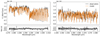 |
Fig. 1 Last two orders (containing CO opacity) of the K-band spectrum of the brown dwarf 2M0355 taken with Keck/NIRSPEC. The orange line is the best-fit model with log(g)=4.69, [Fe/H] = 0.2,C/O = 0.55, and 12CO/13CO = 97, obtained from the maximum likelihood model in the retrieval analysis. The bottom panel shows the residuals of the observed spectrum with respect to the model. |
3 Retrieval analysis
3.1 Atmospheric retrieval model
For our atmospheric free retrieval, in which all fitted parameters varied freely under the condition of chemical equilibrium but the temperaturestructure is unconstrained, we used a Bayesian framework composed of the radiative transfer tool petitRADTRANS (pRT) (Mollière et al. 2019) and the nested sampling tool PyMultiNest (Buchner et al. 2014), which is a Python wrapper of the MultiNest method (Feroz et al. 2009). Synthetic emission spectra are generated by pRT using a set of inputs, including the temperaturestructure, chemical abundances, and surface gravity. The PyMultiNest samples the parameter space and derives the posterior distribution of the fit.
The forward modelling consists of three major components: the temperature model, the chemistry model, and the cloud model. We parameterised the temperature–pressure (T–P) profile using four temperature knots spaced evenly on a log scale pressure within 0.02–5 bar, where the contributionfunction of the observed spectrum peaks (see upper right panel in Fig. 3). The entire T–P profile was obtained by spline interpolation of the four temperature knots in the log space of pressure. The temperature profile outside this range is barely probed by the observations, and is simply considered to be isothermal in our model. There is no physical reasoning behind this T–P profile, and therefore few prior constraints are imposed on the solution.
The chemistry model used in our retrievals assumes chemical equilibrium as detailed in Mollière et al. (2017, 2020). In short, the chemical abundances are determined via interpolation in a chemical equilibrium table using pressure P, temperature T, carbon-to-oxygen ratio C/O, and metallicity [Fe/H] as inputs.
As for the cloud model, the same setup as in Mollière et al. (2020) is implemented using the Ackerman & Marley (2001) model. It introduces four additional free parameters: the mass fraction of the cloud species at the cloud base  , the settling parameter fsed (controlling the thickness of the cloud above the cloud base), the vertical eddy diffusion coefficient Kzz (effectively determining the particle size), and the width of the log-normal particle size distribution σg. The location of the cloud base Pbase is determined by intersecting the condensation curve of the cloud species with the T − P profile of the atmosphere. MgSiO3 and Fe clouds are expected to be the dominant cloud species in L dwarfs (Morley et al. 2012). Here, we only consider the MgSiO3 clouds, because Fe is not expected to be the dominant aerosol composition according to the microphysics model by Gao et al. (2020), and (even if the cloud forms) it condensates at a higher temperature which occurs at lower altitudes than the photosphere of the target.
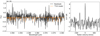 |
Fig. 2 Left panel: observational residuals (observed spectrum minus best-fit model with the 13CO abundance set to zero) in black and 13CO model spectrum given the best-fit 12CO/13CO ratio (~97) in orange. Right panel: cross-correlation function (CCF) between the 13CO model and residuals. The CCF is normalised by its standard deviation within the velocity ranges [−2200, −800] and [800, 2200] km s−1, so that the y-axis represents the signal-to-noise of the CCF peak. |
3.2 Retrieving 2M0355
The cloudy retrieval model has 14 free parameters: Rp, log(g), [Fe/H], C/O, 12CO/13CO,  , fsed, Kzz, σg, vsin(i) and four temperature knots for the T–P profile. The priors of these free parameters are listed in Table 2. We included H2O, CH4, NH3, 12CO, and the isotopologue13CO as line opacityspecies. The model also accounts for the Rayleigh scattering of H2, He, the collision induced absorption of H2 –H2, H2 –He, the scattering and absorption cross sections of crystalline, irregularly shaped MgSiO3 cloud particles.
We used the line-by-line mode of pRT to calculate the emission spectra at high spectral resolution. To speed up the calculation, we took every fifth point of opacity tables with λ∕Δλ ~ 106. This sampling factor of 5 has been benchmarked against the original sampling to ensure unbiased inference of parameters. The synthetic high-resolution spectra were rotationally broadened by vsin(i) and convolved with a Gaussian kernel to match the resolving power of the instrument (λ∕Δλ ~ 27 500), then binned to the wavelength grid of the observed spectrum (2020 data points in total), and scaled to the observed flux according to Rp and distance of the target.
The retrievals were performed by PyMultiNest in importance nested sampling mode with a constant efficiency of 5%. It uses 2000 live points to sample the parameter space and derives the posterior abundances.
Priors and posteriors (90% uncertainties) of the 2M0355 retrievals.
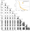 |
Fig. 3 Retrieved parameters and temperature structure of 2M0355 using the nominal model. Upper right panel: retrieved temperature-pressure confidence envelopes. The coloured regions represent 1σ, 2σ, 3σ confidence envelopes. The black dotted line shows the flux average of the emission contribution function. The gray dashed line represents the condensation curve of MgSiO3 clouds. Lower left panel: posterior distributions of parameters. The vertical dashed lines denote the 5%, 50%, 95% quantiles (90% uncertainties) of the distribution. |
4 Results
4.1 Retrieval results
The retrieval results are shown in Fig. 3, including the retrieved temperature-pressure profile and the posterior distribution of the free parameters. The central values of the inferred parameters and their 90% uncertainties are summarised in Table 2, including 12CO/13CO  , C/O
, C/O , [Fe/H]
 , log(g) =
  , and Rp
  . It suggests that 2M0355 has a solar C/O ratio and a super-solar metallicity. The inferred mass of
  MJup is in line with previous estimations using evolutionary models based on its photometry and membership (age) of AB Dor moving group (Faherty et al. 2013). Using the evolutionary models for low-mass objects by Baraffe et al. (2015), we estimate the radius of a ~ 20 MJup dwarf to be ~1.15 RJup for an age of 120 Myr. The radius constrained from our retrieval model (~ 0.97 RJup) is smaller than that expected from evolutionary tracks. This is likely associated with the temperature structure in the retrievalmodels. We note that the alternative retrieval model (described below) converges to different T–P profiles, leading to radii in agreement with the estimation from evolutionary models (see Table 2).
Moreover, we retrieved a much smaller rotational velocity (<4 km s−1) than the value (14.7 km s−1) found by Bryan et al. (2018) using the same data, as listed in Table 1. Broadening synthetic spectra with a vsin(i) of 14.7 km s−1 result in spectral lines too broad to fit the observation with a λ∕Δλ ~ 27 500. In our case, the widths of spectral lines are therefore dominated by the instrument resolution instead of the spin of the target. Regardless, the rotational broadening shows no impact on the inference of the isotopologue ratio.
Figure 3 shows that the properties of clouds are barely constrained. The inferred values of the parameters are similar to the cloud-free case that we tested, indicating that the retrieval converges to solutions with optically thin clouds. We suggest that this behaviour is a cooperative consequence of the freely adjustable temperaturestructure and properties of clouds. Since the presence of thick clouds can block the emission from high-temperature regions of the atmosphere below, the cloudy atmosphere is spectrally equivalent to the case of a cloudless atmosphere combined with a shallow (isothermal) temperature gradient. This effect has been put forward as an alternative (cloud-free) explanation for the red spectra of brown dwarfs and self-luminous exoplanets (Tremblin et al. 2015, 2016, 2017, 2019). Both cases provide good fits to the observed spectrum, but here the free retrieval model tends to converge to cloudless solutions, potentially because they occupy a larger volume in the parameter space than the cloudy solutions. The problem of too isothermal temperature structures in free retrievals of cloudy objects has also been discussed in Burningham et al. (2017), Mollière et al. (2020), and Burningham et al. (2021). Classical 1-d self-consistent calculations will predict a steeper temperature profile, requiring clouds to fit the data. It is therefore important to examine how the inference of other parameters is affected in both cases.
To obtain a more reasonable temperature structure incorporating the effect of clouds, we have to enforce a cloudy atmosphere with a free parameter τcloud, which artificially sets the optical depth of the cloud at the photosphere of the clear component of the atmosphere (where the major emission contribution lies assuming no clouds). In this case, we no longer fit for the cloud mass fraction  . Instead, the optical depth of clouds at all pressure levels is scaled to fulfill the prescribed τcloud. A strict prior is set to enforce optically thick clouds (τcloud > 1). Moreover, we also ensure that the prescribed τcloud is physically plausible by constraining the scaling factor of the cloud optical depth to be less than 2(fsed + 1). This factor fsed + 1 results from the requirement that the cloud surface density (i.e. integrating the product of density with cloud mass fraction vertically) be constrained by the available mass above the cloud base before condensation takes place (i.e. with the equilibrium mass fraction
  ). With the cloud mass fraction depending on the altitude via Xc(P) ∝ Pfsed, this leads to the constraint for the mass fraction at the cloud base:
 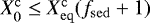 . We added a factor of two to offer some flexibility.
This alternative model results in more pronounced clouds and less isothermal T-P profiles, as is shown in Fig. 4. Comparing the retrieved values of other atmospheric properties (see Table 2), we note that the atmospheric gravity and radius are significantly modified as a result of the heavy cloud and the altered temperature structure. The alternative model no longer probes as deep as the cloudless model because the clouds hide the region below. In addition, the metallicity becomes smaller when clouds are enforced in the retrieval, because the steeper temperature gradient requires less absorbing gas to achieve a similar absorption in emergent flux, as also explained in Burningham et al. (2021). Retrievals over a larger wavelength coverage (in particular, probing silicate absorption features at 10 μm) will reveal the nature of clouds and help better constrain other properties of the atmospheres (Burningham et al. 2021). Nevertheless, it is reassuring that the retrieval of the C/O and 12CO/13CO ratios does not strongly rely on the accurate inference of temperature structure and clouds, which was also found in Mollière et al. (2020) and Burningham et al. (2021).
Results of Bayesian model comparison for the two retrieval models with and without 13CO.
4.2 13CO detection
To reveal the presence of 13CO signal, we compare the observed spectrum to the retrieved best-fit model (log(g) = 4.69, [Fe/H] = 0.2, C/O = 0.55, and 12CO/13CO = 97) in Fig. 1, and calculate the cross-correlation function (CCF) between the residuals (the observed spectrum minus the best-fit model without 13CO) and a 13CO model (Fig. 2). The 13CO model spectrum is constructed by taking the difference between the best-fit model and the same model with the 13CO abundance set to zero. As is shown in the right panel of Fig. 2, the CCF peaks at zero radial velocity, signifying the detection of 13CO at an S/N of 8.4. This value varies slightly depending on the choice of velocity ranges where the standard deviation of the noise is measured.
We also determined the significance of the 13CO detection using Bayesian model selection. We performed the retrieval again while excluding 13CO opacity and the parameter 12CO/13CO. Comparing its Bayesian evidence (Z) to that of the full model (as listed in Table 3) allows us to assess the extent to which the model including 13CO is favoured by the observations. In Bayesian model comparison, the Bayes factor Bm (calculated by the ratio of Z) is used as a proxy for the posterior odds ratio between two models. We then translated Bm to the frequentist measures of significance following Benneke & Seager (2013). As a result, the difference of ln (Z) between two models is Δ ln (Z) = ln(Bm) = 44, meaning that the observation favours the full model (including 13CO) at a significance level of 9.5σ. The detection remains the same significance (9.5σ) when we use the alternative model with enhanced clouds.
5 Discussion
5.1 CO isotopologue ratio in 2M0355
We found the CO isotopologue ratio in 2M0355 (12CO/13CO =  ) to be similar to the carbon isotope ratio measured in for the Sun (93.5 ± 3 by Lyons et al. 2018), while it is marginally higher than the ratio in today’s local ISM (68 ± 15 by Milam et al. 2005), which is expected to be inherited by young objects. However, recent measurements of carbon isotope ratios towards a sample of solar twins suggest a current local value of ~ 81.3 (Botelho et al. 2020), which is within the uncertainty of our measurement. Therefore, it remains unclear whether the CO isotopologueratio in 2M0355 is indeed higher than its local environment.
We note that high 12CO/13CO ratios were also observed towards some diffuse clouds, molecular clouds and YSOs in the solar neighbourhood (Lambert et al. 1994; Federman et al. 2003; Goto et al. 2003; Smith et al. 2015). If the high 12CO/13CO ratios in molecular clouds and YSOs do not result from observational biases, it may not be surprising that the brown dwarf 2M0355 might inherit the high ratio from a 13CO-diminished parent cloud. One possible explanation for the high ratios towards diffuse clouds is the isotope-selective photodissociation (Bally & Langer 1982; van Dishoeck & Black 1988; Visser et al. 2009). Because of the lower column density of the rarer isotopologue, the self-shielding of 13CO takes effect at a deeper layer in the cloud.Consequently, 13CO is preferably destructed by far-ultraviolet (FUV) radiation, increasing the 12CO/13CO ratios in the ISM. However, this explanation is not as plausible for molecular clouds and YSOs, because these objects with high extinction are supposed to be well shielded from FUV radiation. The isotope-selective photodissociation is unlikely to significantly alter the globally isotopologue ratios (van Dishoeck & Black 1988). Other hypotheses were also suggested, such as higher excitation temperature in 12CO than in 13CO resulted from photon trapping in 12CO rotational transitions (Goto et al. 2003), CO gas-to-ice reservoir partitioning (Smith et al. 2015), and ISM enrichment caused by ejecta from carbon-rich giant stars or supernovae (Crossfield et al. 2019), but no general and conclusive interpretation.
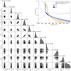 |
Fig. 4 Similar to Fig. 3, but for the alternative model with enforced clouds. Upper right panel compares the temperature-pressure profiles of the nominal model in Fig. 3 (in orange) to this alternative model (in blue). |
5.2 Implications for planet formation
It is intriguing to compare the 12CO/13CO measurements between the L dwarf 2M0355 (~97) and the wide-orbit exoplanet TYC 8998 b (~31 by Zhang et al. 2021). Despite similarities in several aspects, the young super-Jupiter has possibly undergone a different formation pathway to the isolated brown dwarf, leading to the difference in isotopologue ratio in their atmospheres. While isolated brown dwarfs may experience a top-down formation via gravitational collapse (which resembles star formation) or disk instability (Boss 1997; Kratter & Lodato 2016), super-Jupiters possibly form through the bottom-up core-accretion (of planetesimals and pebbles) (Pollack et al. 1996; Lambrechts & Johansen 2012). Previous demographics on giant planets and brown dwarfs (Nielsen et al. 2019; Bowler et al. 2020) also support the two distinct formation pathways. As argued in Zhang et al. (2021), the core-accretion scenario could possibly lead to 13CO enrichment through ice accretion, lowering the 12CO/13CO ratio in observed super-Jupiter atmospheres.
Admittedly, it is preliminary to draw any conclusive interpretation based on a sample of two objects. Another caveat is that the two measurements towards the super-Jupiter and the L dwarf are carried out under different spectral resolutions. It is so far unclear whether a smaller spectral resolving power can lead to any observational biases because it probes unresolved molecular lines. This calls for more future observations that enable homogeneous comparisonsbetween different objects, in order to better understand the potential and limitations of carbon isotopologue ratio as a tracer for planet formation. It is also essential to interpret the isotopologue measurements in light of carbon fractionation in protoplanetary disks (Miotello et al. 2014), disk evolution (Trapman et al. 2021), CO ice chemistry (Krijt et al. 2020), and planet formation (Cridland et al. 2020), in order to provide constraints on the birth location, the relative importance of ice accretion, and possible vertical gas accretion processes during formation.
6 Conclusion
We analysed archival high-resolution spectra (from 2.275 to 2.385 μm) from Keck/NIRSPEC of the isolated brown dwarf 2M0335 and carried out a free retrieval analysis. After removing the retrieved best-fit model that includes only the main isotopologues, we detected a 13CO signal using the cross-correlation method with an S/Nof ~8.4. The detection significance was determined to be ~9.5σ with a Bayesian model comparison between the two retrieval models including or excluding 13CO. The isotopologue ratio 12CO/13CO is inferred to be  , similar to the value found in the Sun, while marginally higher than the local ISM standard. If this deviation is real, it is possibly inherited from its parent cloud that has a high 12CO/13CO ratio.
Although based on only two objects, it is also intriguing to note the difference between carbon isotopologue ratios in giant exoplanets and brown dwarfs, potentially implying distinct formation pathways. Despite spectroscopic similarities, brown dwarfs may experience a top-down formation via gravitational collapse, which resembles star formation, while giant exoplanets likely form through a bottom-up accretion process, which may alter isotopologue ratios in their atmospheres with dependencies on the accretion location and pathway in protoplanetary disks. This further emphasises the atmospheric carbon isotopologue ratio as a tracer for planet formation history. In the future, such an analysis can be implemented on spectra of more exoplanets to measure the carbon isotopologue ratios in their atmospheres and shed light on the location and mechanisms of planet formation.
Acknowledgements
We thank the referee and editor for helpful comments. This research has made use of the Keck Observatory Archive (KOA), which is operated by the W.M. Keck Observatory and the NASA Exoplanet Science Institute (NExScI), under contract with the National Aeronautics and Space Administration. This work was performed using the compute resources from the Academic Leiden Interdisciplinary Cluster Environment (ALICE) provided by Leiden University. Y.Z. and I.S. acknowledge funding from the European Research Council (ERC) under the European Union’s Horizon 2020 research and innovation program under grant agreement no. 694513. P.M. acknowledges support from the European Research Council under the European Union’s Horizon 2020 research and innovation program under grant agreement no. 832428.
References
- Acharyya, K., Fuchs, G. W., Fraser, H. J., van Dishoeck, E. F., & Linnartz, H. 2007, A&A, 466, 1005 [NASA ADS] [CrossRef] [EDP Sciences] [Google Scholar]
- Ackerman, A. S., & Marley, M. S. 2001, ApJ, 556, 872 [Google Scholar]
- Aller, K. M., Liu, M. C., Magnier, E. A., et al. 2016, ApJ, 821, 120 [NASA ADS] [CrossRef] [Google Scholar]
- Altwegg, K., Balsiger, H., Bar-Nun, A., et al. 2015, Science, 347, 1261952 [Google Scholar]
- Bally, J., & Langer, W. D. 1982, ApJ, 255, 143 [NASA ADS] [CrossRef] [Google Scholar]
- Baraffe, I., Homeier, D., Allard, F., & Chabrier, G. 2015, A&A, 577, A42 [NASA ADS] [CrossRef] [EDP Sciences] [Google Scholar]
- Benneke, B., & Seager, S. 2013, ApJ, 778, 153 [Google Scholar]
- Blake, C. H., Charbonneau, D., & White, R. J. 2010, ApJ, 723, 684 [Google Scholar]
- Boogert, A. C. A., Tielens, A. G. G. M., Ceccarelli, C., et al. 2000, A&A, 360, 683 [NASA ADS] [Google Scholar]
- Boogert, A. C. A., Blake, G. A., & Tielens, A. G. G. M. 2002, ApJ, 577, 271 [NASA ADS] [CrossRef] [Google Scholar]
- Boss, A. P. 1997, Science, 276, 1836 [Google Scholar]
- Botelho, R. B., Milone, A. d. C., Meléndez, J., et al. 2020, MNRAS, 499, 2196 [CrossRef] [Google Scholar]
- Bowler, B. P., Blunt, S. C., & Nielsen, E. L. 2020, AJ, 159, 63 [Google Scholar]
- Bryan, M. L., Benneke, B., Knutson, H. A., Batygin, K., & Bowler, B. P. 2018, Nat. Astron., 2, 138 [Google Scholar]
- Buchner, J., Georgakakis, A., Nandra, K., et al. 2014, A&A, 564, A125 [NASA ADS] [CrossRef] [EDP Sciences] [Google Scholar]
- Burningham, B., Marley, M. S., Line, M. R., et al. 2017, MNRAS, 470, 1177 [NASA ADS] [CrossRef] [Google Scholar]
- Burningham, B., Faherty, J. K., Gonzales, E. C., et al. 2021, MNRAS, 506, 1944 [NASA ADS] [CrossRef] [Google Scholar]
- Clayton, D. D., & Nittler, L. R. 2004, ARA&A, 42, 39 [NASA ADS] [CrossRef] [Google Scholar]
- Cridland, A. J., Bosman, A. D., & van Dishoeck, E. F. 2020, A&A, 635, A68 [NASA ADS] [CrossRef] [EDP Sciences] [Google Scholar]
- Crossfield, I. J. M., Lothringer, J. D., Flores, B., et al. 2019, ApJ, 871, L3 [NASA ADS] [CrossRef] [Google Scholar]
- Cruz, K. L., Kirkpatrick, J. D., & Burgasser, A. J. 2009, AJ, 137, 3345 [NASA ADS] [CrossRef] [Google Scholar]
- Cutri, R. M., Skrutskie, M. F., van Dyk, S., et al. 2003, VizieR Online Data Catalog: II/246 [Google Scholar]
- Drake, M. J. 2005, Meteor. Planet. Sci., 40, 519 [NASA ADS] [CrossRef] [Google Scholar]
- Faherty, J. K., Rice, E. L., Cruz, K. L., Mamajek, E. E., & Núñez, A. 2013, AJ, 145, 2 [CrossRef] [Google Scholar]
- Federman, S. R., Lambert, D. L., Sheffer, Y., et al. 2003, ApJ, 591, 986 [NASA ADS] [CrossRef] [Google Scholar]
- Feroz, F., Hobson, M. P., & Bridges, M. 2009, MNRAS, 398, 1601 [NASA ADS] [CrossRef] [Google Scholar]
- Feuchtgruber, H., Lellouch, E., Orton, G., et al. 2013, A&A, 551, A126 [NASA ADS] [CrossRef] [EDP Sciences] [Google Scholar]
- Gaia Collaboration (Brown, A. G. A. et al.) 2018, A&A, 616, A1 [NASA ADS] [CrossRef] [EDP Sciences] [Google Scholar]
- Gao, P., Thorngren, D. P., Lee, G. K. H., et al. 2020, Nat. Astron., 4, 951 [NASA ADS] [CrossRef] [Google Scholar]
- Goto, M., Usuda, T., Takato, N., et al. 2003, ApJ, 598, 1038 [NASA ADS] [CrossRef] [Google Scholar]
- Horne, K. 1986, PASP, 98, 609 [Google Scholar]
- Husser, T. O., Wende-von Berg, S., Dreizler, S., et al. 2013, A&A, 553, A6 [NASA ADS] [CrossRef] [EDP Sciences] [Google Scholar]
- Jones, A., Noll, S., Kausch, W., Szyszka, C., & Kimeswenger, S. 2013, A&A, 560, A91 [NASA ADS] [CrossRef] [EDP Sciences] [Google Scholar]
- Jørgensen, J. K., van der Wiel, M. H. D., Coutens, A., et al. 2016, A&A, 595, A117 [Google Scholar]
- Jørgensen, J. K., Müller, H. S. P., Calcutt, H., et al. 2018, A&A, 620, A170 [Google Scholar]
- Kratter, K., & Lodato, G. 2016, ARA&A, 54, 271 [NASA ADS] [CrossRef] [Google Scholar]
- Krijt, S., Bosman, A. D., Zhang, K., et al. 2020, ApJ, 899, 134 [NASA ADS] [CrossRef] [Google Scholar]
- Lambert, D. L., Sheffer, Y., Gilliland, R. L., & Federman, S. R. 1994, ApJ, 420, 756 [NASA ADS] [CrossRef] [Google Scholar]
- Lambrechts, M., & Johansen, A. 2012, A&A, 544, A32 [NASA ADS] [CrossRef] [EDP Sciences] [Google Scholar]
- Langer, W. D., & Penzias, A. A. 1993, ApJ, 408, 539 [NASA ADS] [CrossRef] [Google Scholar]
- Langer, W. D., Graedel, T. E., Frerking, M. A., & Armentrout, P. B. 1984, ApJ, 277, 581 [Google Scholar]
- Liu, M. C., Dupuy, T. J., & Allers, K. N. 2013, Astron. Nachr., 334, 85 [NASA ADS] [CrossRef] [Google Scholar]
- Lyons, J. R., Gharib-Nezhad, E., & Ayres, T. R. 2018, Nat. Commun., 9, 908 [Google Scholar]
- Madhusudhan, N., Amin, M. A., & Kennedy, G. M. 2014, ApJ, 794, L12 [Google Scholar]
- McLean, I. S., Becklin, E. E., Bendiksen, O., et al. 1998, in Society of Photo-Optical Instrumentation Engineers (SPIE) Conference Series, 3354, Infrared Astronomical Instrumentation, ed. A. M. Fowler, 566 [Google Scholar]
- Milam, S. N., Savage, C., Brewster, M. A., Ziurys, L. M., & Wyckoff, S. 2005, ApJ, 634, 1126 [Google Scholar]
- Miotello, A., Bruderer, S., & van Dishoeck, E. F. 2014, A&A, 572, A96 [NASA ADS] [CrossRef] [EDP Sciences] [Google Scholar]
- Mollière, P., & Snellen, I. A. G. 2019, A&A, 622, A139 [NASA ADS] [CrossRef] [EDP Sciences] [Google Scholar]
- Mollière, P., van Boekel, R., Bouwman, J., et al. 2017, A&A, 600, A10 [Google Scholar]
- Mollière, P., Wardenier, J. P., van Boekel, R., et al. 2019, A&A, 627, A67 [Google Scholar]
- Mollière, P., Stolker, T., Lacour, S., et al. 2020, A&A, 640, A131 [Google Scholar]
- Mordasini, C., van Boekel, R., Mollière, P., Henning, T., & Benneke, B. 2016, ApJ, 832, 41 [Google Scholar]
- Morley, C. V., Fortney, J. J., Marley, M. S., et al. 2012, ApJ, 756, 172 [NASA ADS] [CrossRef] [Google Scholar]
- Morley, C. V., Skemer, A. J., Miles, B. E., et al. 2019, ApJ, 882, L29 [NASA ADS] [CrossRef] [Google Scholar]
- Nielsen, E. L., De Rosa, R. J., Macintosh, B., et al. 2019, AJ, 158, 13 [Google Scholar]
- Noll, S., Kausch, W., Barden, M., et al. 2012, A&A, 543, A92 [NASA ADS] [CrossRef] [EDP Sciences] [Google Scholar]
- Öberg, K. I., Murray-Clay, R., & Bergin, E. A. 2011, ApJ, 743, L16 [Google Scholar]
- Pollack, J. B., Hubickyj, O., Bodenheimer, P., et al. 1996, Icarus, 124, 62 [NASA ADS] [CrossRef] [Google Scholar]
- Pontoppidan, K. M., Dullemond, C. P., van Dishoeck, E. F., et al. 2005, ApJ, 622, 463 [NASA ADS] [CrossRef] [Google Scholar]
- Reid, I. N., Cruz, K. L., Kirkpatrick, J. D., et al. 2008, AJ, 136, 1290 [Google Scholar]
- Smette, A., Sana, H., Noll, S., et al. 2015, A&A, 576, A77 [NASA ADS] [CrossRef] [EDP Sciences] [Google Scholar]
- Smith, R. L., Pontoppidan, K. M., Young, E. D., & Morris, M. R. 2015, ApJ, 813, 120 [NASA ADS] [CrossRef] [Google Scholar]
- Sneden, C., Pilachowski, C. A., & Vandenberg, D. A. 1986, ApJ, 311, 826 [NASA ADS] [CrossRef] [Google Scholar]
- Trapman, L., Bosman, A. D., Rosotti, G., Hogerheijde, M. R., & van Dishoeck, E. F. 2021, A&A, 649, A95 [EDP Sciences] [Google Scholar]
- Tremblin, P., Amundsen, D. S., Mourier, P., et al. 2015, ApJ, 804, L17 [CrossRef] [Google Scholar]
- Tremblin, P., Amundsen, D. S., Chabrier, G., et al. 2016, ApJ, 817, L19 [NASA ADS] [CrossRef] [Google Scholar]
- Tremblin, P., Chabrier, G., Baraffe, I., et al. 2017, ApJ, 850, 46 [CrossRef] [Google Scholar]
- Tremblin, P., Padioleau, T., Phillips, M. W., et al. 2019, ApJ, 876, 144 [Google Scholar]
- Tsuji, T. 2016, PASJ, 68, 84 [NASA ADS] [CrossRef] [Google Scholar]
- van Dishoeck, E. F., & Black, J. H. 1988, ApJ, 334, 771 [Google Scholar]
- Visser, R., van Dishoeck, E. F., & Black, J. H. 2009, A&A, 503, 323 [NASA ADS] [CrossRef] [EDP Sciences] [Google Scholar]
- Woods, P. M. 2009, ArXiv e-prints, [arXiv:0901.4513] [Google Scholar]
- Yan, Y. T., Zhang, J. S., Henkel, C., et al. 2019, ApJ, 877, 154 [Google Scholar]
- Zhang, Y., Snellen, I. A. G., Bohn, A. J., et al. 2021, Nature, 595, 370 [NASA ADS] [CrossRef] [Google Scholar]
All Tables
Results of Bayesian model comparison for the two retrieval models with and without 13CO.
All Figures
|
Fig. 1 Last two orders (containing CO opacity) of the K-band spectrum of the brown dwarf 2M0355 taken with Keck/NIRSPEC. The orange line is the best-fit model with log(g)=4.69, [Fe/H] = 0.2,C/O = 0.55, and 12CO/13CO = 97, obtained from the maximum likelihood model in the retrieval analysis. The bottom panel shows the residuals of the observed spectrum with respect to the model. |
| In the text | |
|
Fig. 2 Left panel: observational residuals (observed spectrum minus best-fit model with the 13CO abundance set to zero) in black and 13CO model spectrum given the best-fit 12CO/13CO ratio (~97) in orange. Right panel: cross-correlation function (CCF) between the 13CO model and residuals. The CCF is normalised by its standard deviation within the velocity ranges [−2200, −800] and [800, 2200] km s−1, so that the y-axis represents the signal-to-noise of the CCF peak. |
| In the text | |
|
Fig. 3 Retrieved parameters and temperature structure of 2M0355 using the nominal model. Upper right panel: retrieved temperature-pressure confidence envelopes. The coloured regions represent 1σ, 2σ, 3σ confidence envelopes. The black dotted line shows the flux average of the emission contribution function. The gray dashed line represents the condensation curve of MgSiO3 clouds. Lower left panel: posterior distributions of parameters. The vertical dashed lines denote the 5%, 50%, 95% quantiles (90% uncertainties) of the distribution. |
| In the text | |
|
Fig. 4 Similar to Fig. 3, but for the alternative model with enforced clouds. Upper right panel compares the temperature-pressure profiles of the nominal model in Fig. 3 (in orange) to this alternative model (in blue). |
| In the text | |
Current usage metrics show cumulative count of Article Views (full-text article views including HTML views, PDF and ePub downloads, according to the available data) and Abstracts Views on Vision4Press platform.
Data correspond to usage on the plateform after 2015. The current usage metrics is available 48-96 hours after online publication and is updated daily on week days.
Initial download of the metrics may take a while.