| Issue |
A&A
Volume 707, March 2026
|
|
|---|---|---|
| Article Number | A210 | |
| Number of page(s) | 15 | |
| Section | Planets, planetary systems, and small bodies | |
| DOI | https://doi.org/10.1051/0004-6361/202558089 | |
| Published online | 17 March 2026 | |
The ESO SupJup Survey
IX. Isotopic evidence of a recent formation for Luhman 16AB
1
Leiden Observatory, Leiden University,
PO Box 9513,
2300 RA,
Leiden,
The Netherlands
2
Department of Physics, University of Warwick,
Coventry
CV4 7AL,
UK
3
Centre for Exoplanets and Habitability, University of Warwick,
Gibbet Hill Road,
Coventry
CV4 7AL,
UK
4
IPAC,
Mail Code 100-22, Caltech, 1200 E. California Boulevard,
Pasadena,
CA
91125,
USA
5
Max-Planck-Institut für Astronomie,
Königstuhl 17,
69117
Heidelberg,
Germany
6
School of Physics, Trinity College Dublin, University of Dublin,
Dublin 2,
Ireland
7
Department of Astronomy, California Institute of Technology,
Pasadena,
CA
91125,
USA
★ Corresponding author: This email address is being protected from spambots. You need JavaScript enabled to view it.
Received:
13
November
2025
Accepted:
28
January
2026
Abstract
Context. The distinct formation pathways proposed for directly imaged exoplanets and isolated brown dwarfs might leave imprints in the inherited chemical composition. Elemental and isotopic tracers could help inform the suspected histories, but this requires a careful characterisation of the sub-stellar atmospheres. In particular, objects at the L-T transition exhibit signs of dynamics that can drive their atmospheres out of chemical equilibrium.
Aims. In this work, we studied the nearest L-T brown dwarfs, Luhman 16A and B, to assess the chemical disequilibrium in their atmospheres. We also investigated the elemental and isotopic compositions in the context of their probable formation history within the Oceanus moving group.
Methods. As part of the ESO SupJup Survey, we obtained spatially resolved CRIRES+ K-band spectra of the binary. These high-resolution observations were analysed using an atmospheric retrieval framework that couples the radiative transfer code petitRADTRANS to the MultiNest sampling algorithm.
Results. We detect and retrieve the abundances of 12CO, H2O, CH4, NH3, H2S, HF, and the 13CO isotopologue. We find that both atmospheres are in chemical disequilibrium with somewhat stronger vertical mixing in Luhman 16A compared to B (Kzz,A ~ 108.7 vs Kzz,B ~ 108.2 cm2 s−1). The tested chemical models, free-equilibrium and disequilibrium chemistry, yield consistent mixing ratios and agree with earlier work at shorter wavelengths. The free-chemistry gaseous C/O ratios show evidence of oxygen trapping in silicate-oxide clouds. While the C/O ratios are consistent with the solar composition, the metallicities are modestly enhanced with [C/H] ~ 0.15. The carbon isotope ratios are measured at 12C/13CA = 74−2+2 and 2C/13CB = 74−3+3.
Conclusions. The coincident constraints of metallicities and isotopes across the binary provide further evidence in favour of a common formation. The 12C/13C ratios are aligned with the present-day interstellar medium but lower than the Solar System value. This suggests a recent inheritance and corroborates the relatively young age (~500 Myr) of Luhman 16A and B as members of the Oceanus moving group.
Key words: techniques: spectroscopic / planets and satellites: atmospheres / brown dwarfs
© The Authors 2026
 Open Access article, published by EDP Sciences, under the terms of the Creative Commons Attribution License (https://creativecommons.org/licenses/by/4.0), which permits unrestricted use, distribution, and reproduction in any medium, provided the original work is properly cited.
This article is published in open access under the Subscribe to Open model. This email address is being protected from spambots. You need JavaScript enabled to view it. to support open access publication.
1 Introduction
Brown dwarfs at the transition between spectral types L and T go through a remarkable change in their spectro-photometric appearance (Kirkpatrick 2005). The cooler T dwarfs exhibit a shift towards bluer colours, which has often been associated with the dissipation of photospheric clouds (e.g. Burrows et al. 2006; Saumon & Marley 2008) as well as thermo-chemical instabilities (Tremblin et al. 2016). In this temperature regime (1200-1400 K; Faherty et al. 2014), the sub-stellar objects also experience a transition in their atmospheric chemistry. The higher L-dwarf temperatures favour CO as the main carbonbearing species, while the T-type dwarfs are defined by the strengthening CH4 absorption in their spectra (Cushing et al. 2005; Kirkpatrick 2005). The observables are further impacted by atmospheric dynamics that likely drive the photometric variability that is commonly seen for L-T objects (Radigan et al. 2014). In addition, strong vertical mixing within the atmosphere inhibits the conversion of CO into CH4 at low pressures (Hubeny & Burrows 2007; Zahnle & Marley 2014; Mukherjee et al. 2022). The resulting chemical disequilibrium can be assessed through measurements of under-abundant CH4 or enhanced CO absorption (e.g. Noll et al. 1997; Geballe et al. 2009; Miles et al. 2020).
Directly imaged exoplanets and isolated brown dwarfs share similar atmospheric temperatures and, by extension, are in comparable chemical states (Faherty et al. 2016). The two populations likely have distinct formation histories, resulting in differences in the accreted elemental abundances. The composition of giant exoplanets is thought to be imprinted with the chemical and isotopic fractionation that occurs at various radii throughout the circumstellar disc (Öberg & Bergin 2021 ; Bergin et al. 2024). Isolated brown dwarfs, on the other hand, form via gravitational collapse, and their compositions are expected to reflect the chemical content of the parent molecular cloud (Bate et al. 2002; Chabrier et al. 2014). Elemental abundance ratios such as the C/O, N/O, and refractory-to-volatile ratios have been suggested as valuable planet-formation tracers (Öberg et al. 2011; Madhusudhan 2012; Turrini et al. 2021; Lothringer et al. 2021), but isotope ratios have been proposed as complementary tracers as well (Mollière & Snellen 2019; Morley et al. 2019). The carbon isotope ratio, 12C∕13C, may be particularly useful for assessing the formation epochs of brown dwarfs and low-mass stars. Owing to their fully convective interiors and lack of carbon production, their atmospheres preserve the 12C/13C ratio of their natal environments. While stars ultimately expel both isotopes back into the interstellar medium (ISM), they have separate nucleosynthetic origins, with 12C synthesised in the triple-α process and 13C created as a secondary element through the CNO cycle (Wiescher et al. 2010). As such, the 12C/13C ratio is expected to decrease over time as the necessary metals for the CNO cycle become accessible (Romano 2022). In agreement with predictions of galactic chemical evolution, González Picos et al. (2025b) find that nearby M-dwarf stars with increased metallicities are also progressively enriched in 13C.
The WISE J104915.57-531906.1 system, or Luhman 16, is the nearest brown dwarf binary, at a distance of ~2 pc (Luhman 2013; Bedin et al. 2024). The primary and secondary components, A and B, are classified, respectively, as L7.5 and T0.5±1.0 (Burgasser et al. 2013). Coincidentally, the kinematic motion of Luhman 16AB yields an association with Oceanus, a moving group with an estimated age of ~500 Myr (Gagné et al. 2023). The high apparent brightnesses of the two objects have led to numerous observations, which in turn have been used to characterise their orbits (e.g. Lazorenko & Sahlmann 2018; Bedin et al. 2024), polarisation (Millar-Blanchaer et al. 2020), variabilities (e.g. Biller et al. 2013, 2024; Buenzli et al. 2015b; Fuda et al. 2024; Chen et al. 2025), and spectral energy distributions (e.g. Faherty et al. 2014; Crossfield et al. 2014; Lodieu et al. 2015; Kellogg et al. 2017; Chen et al. 2025; Ishikawa et al. 2025). Given their status as benchmark L-T objects, Luhman 16A and B are well-suited targets for studying the presence of chemical dis-equilibria. Additionally, measurements of elemental and isotopic compositions can provide further constraints on the suspected formation of the binary.
In this paper we present an analysis of the atmospheric chemistry of Luhman 16AB using high-resolution K-band spectra. Section 2 describes the reduction of our observations and the modelling framework that was used to infer the atmospheric properties. Section 3 outlines the results, and Sect. 4 discusses them in the context of previous studies as well as the implied formation history of Luhman 16AB. In Sect. 5, we summarise the conclusions drawn from this atmospheric retrieval analysis.
2 Methods
2.1 Observations and reduction
We observed the Luhman 16 binary as part of the ESO SupJup Survey (programme ID: 110.23RW; see de Regt et al. 2024) on January 1, 2023, using the CRyogenic high-resolution InfraRed Echelle Spectrograph (CRIRES+; Dorn et al. 2023). The K2166 wavelength setting was employed to ensure coverage of the 13CO (ν = 2-0) band head. A single nodding cycle (4 × 300 s) with the 0.4" slit resulted in a signal-to-noise of 400 and 300 (at ~2345 nm), respectively for Luhman 16A and B. These K-band observations were taken prior to the J-band spectra studied in de Regt et al. (2025b). Following a similar reduction procedure using excalibuhr1 (Zhang et al. 2024), we extracted the spectra of each component separately. The optical seeing of ~0.8" and a projected separation of ~0.81" (Bedin et al. 2024) resulted in a degree of blending of the two spectral traces. We applied a correction for the contamination in the 12-pixel wide extraction apertures, following Appendix A of de Regt et al. (2025b). Our K-band observations from the preceding night, December 31, 2022, suffered from worse seeing (~1.5") where the binary components could not be spatially resolved. While it is possible to separate them via their radial and rotational velocities, inferring distinct atmospheric properties proved challenging, and we therefore only studied the observations from the second night.
The standard star HD 93563 was observed with the same settings and reduced in a similar manner. We applied molecfit (Smette et al. 2015) to the standard star spectrum to model the telluric transmission. The obtained model is subsequently used to correct the telluric absorption lines in the Luhman 16AB spectra. We masked out pixels with a transmissivity below T <−80%, as the deepest tellurics are generally poorly fit. Molecfit used first-degree polynomials to fit the continuum, which we divided by the Planck curve corresponding to the standard star (Teff = 15 000 K; Arcos et al. 2018). The Luhman 16 spectra were subsequently corrected for this wavelength-dependent throughput. Since molecfit also fits the telluric line-widths, we obtained an estimated resolution of R ~ 60000 (~5 km s−1), which we used to apply instrumental broadening to the model spectra.
For plotting purposes, we flux-calibrated the Luhman 16 spectra to match the broadband photometry (KA = 9.44 ± 0.07 and KB = 9.73 ± 0.09 mag; Burgasser et al. 2013). Figure 1 shows the calibrated spectra of Luhman 16A and B. The high spectral resolution gives a somewhat noisy appearance in the upper panel, but the zoomed-in panels highlight the superb quality of these observations. The K2166 wavelength setting covers seven spectral orders, measured on three detectors, resulting in 7 ∙ 3 = 21 order-detector pairs, orchips. The upper panel of Fig. 1 shows that the bluest chips have few usable pixels remaining after the telluric masking.
2.2 Retrieval framework
We employed a retrieval framework to constrain the atmospheric properties of the Luhman 16 binary. The radiative transfer code petitRADTRANS (pRT; version 3.1; Mollière et al. 2019, 2020; Blain et al. 2024) is used to generate emission spectra from a set of variables and parameterisations, which are sampled with the PyMultiNest nested sampling algorithm (Feroz et al. 2009; Buchner et al. 2014). We used 1000 live points at a constant sampling efficiency of 5% to run the retrievals. The retrieved parameters and their priors are summarised in Table C.1.
2.2.1 Likelihood and covariance
Following de Regt et al. (2025b), we defined the likelihood as
 (1)
(1)
where the sum is performed over 21 order-detector pairs i that have Ni valid pixels (2048 at most). For each chip, Σ0,i is the un-scaled covariance matrix and ri is the residual between the data di and model mi, calculated as ri = di - φimi. The flux-and covariance-scaling parameters, φi and  , are optimised at each model evaluation using Eqs. (4) and (5) of de Regt et al. (2025b). Similarly, we modelled correlated noise using a Gaussian process amplitude, a, and length-scale, l (Eq. (6) of de Regt et al. 2025b).
 |
Fig. 1 CRIRES+ K-band spectra of Luhman 16A and B in orange and blue, respectively. Top panel : seven spectral orders covered in the K2166 wavelength setting. The telluric absorption is shown as transparent lines. Lower panels : zoom-in of the sixth order. The black observed spectra are overlaid with the best-fitting free-chemistry models in orange and blue. The mean scaled uncertainties are displayed to the right of the residuals in the bottom panel. The fits to the other spectral orders can be found in Appendix D. |
2.2.2 Surface gravity, temperature profile, and clouds
The well-constrained dynamical masses of MA = 35.4 ± 0.2 and MB = 29.4 ± 0.2 MJup (Bedin et al. 2024) were used as prior information. Combined with radii estimates of R = 1.0 ± 0.1 RJup (Biller et al. 2024), this results in Gaussian priors of log gA = 4.96 ± 0.09 and log gB = 4.88 ± 0.09 on the surface gravities.
We adopted the gradient-based parameterisation of the temperature profile described in de Regt et al. (2025b) and introduced by Zhang et al. (2023). This parameterisation is flexible but also produces physically reasonable profiles by way of the chosen priors for the temperature gradients, ∇i (see Table C.1).
As in de Regt et al. (2025b), we used a grey-cloud parameterisation with an opacity κcl,0 at a pressure Pcl,0. Above this cloud base, the opacity decays with the power fsed.
2.2.3 Chemistry
We compared two approaches to modelling the atmospheric chemistries. Firstly, in the free-chemistry approach, we fitted for the abundance of each included species separately. These volume-mixing ratios (VMRs) were assumed to be vertically constant to minimise the number of free parameters. This is a reasonable assumption for this work, as the species encountered in the K band generally do not show a strong depletion through rainout and vertical mixing also helps homogenise their abundances. We included molecular opacity from 12CO, 13CO, C18O, C17O (Li et al. 2015), H2O (Polyansky et al. 2018), H218O, H217O (Polyansky et al. 2017), CH4 (Yurchenko et al. 2024), CO2 (Hargreaves et al. 2025), NH3 (Al Derzi et al. 2015; Coles et al. 2019), HCN (Harris et al. 2006; Barber et al. 2014), H2S (Azzam et al. 2016; Chubb et al. 2018), and HF (Li et al. 2013; Coxon & Hajigeorgiou 2015; Somogyi et al. 2021), calculated with pyROX2 (de Regt et al. 2025a). To clarify, we refer to the main isotope when the mass number superscript is omitted.
In the second model, we simulated atmospheres in chemical disequilibrium using the FastChem Cond code (Kitzmann et al. 2024). Equilibrium-chemistry calculations are generally not fast enough to be performed for each sample during a retrieval, especially when accounting for condensation. However, reducing the considered gases and condensates to only those with appreciable abundances (Table B.1) can bring computation times down to a few tenths of a second with a negligible loss of accuracy, as demonstrated in Appendix B. This model allowed us to compute gaseous VMRs on the fly and include rainout condensation, and we could directly fit for the elemental abundances via [C/H], [O/H], [N/H], [S/H], and [F/H] (relative to the solar composition of Asplund et al. 2021). Five isotopologue ratios are retrieved to derive the abundances of 13CO, C18O, C17O, H218O, and H217O with respect to the main isotopologue. Finally, the abundances of H2O, CH4, CO, NH3, HCN, CO2, and their isotopologues are quenched, or held constant, at P <−Pquench. These quench points are located where the vertical-mixing timescale, tmix, is equal to the chemical timescale of the relevant reaction network (e.g. tCO-CH4-H2O), which we adopted from Zahnle & Marley (2014). The mixing timescale is calculated as
 (2)
(2)
where the length scale, L, is defined as the product of the scale height, H, and a factor, α, allowing mixing lengths to be shorter than the scale height (Smith 1998; Ackerman & Marley 2001). In this work, we assumed α = 1 so that any overestimation of the length scale translates into the vertical eddy diffusion coefficient, Kzz, which is retrieved as a free parameter. The mixing timescale further depends on the temperature profile, mean molecular weight, and surface gravity, which also vary with each evaluated model.
3 Results
The retrieval model provides a good fit to the spectra of Luh-man 16AB, as is demonstrated in the lower panels of Fig. 1. The spectral fits to the remaining six orders can be found in Appendix D. In general, the residuals are contained within the expected uncertainties (indicated as error bars), with the exception of telluric-dominated wavelengths at the longest K-band wavelengths.
3.1 Detection of species
We confirmed the presence of H2O and 12CO from a visual inspection of the absorption features (i.e. Fig. 1). A more detailed investigation was required to report detections of the less abundant species. Hence, we carried out a cross-correlation analysis between the residuals of a model without species X (mi,w/o X) and a template of the contribution from X (mi - mi,w/o X). The crosscorrelation coefficient at a velocity v was then summed over the chips via
 (3)
(3)
The cross-correlation functions (CCFs) were subsequently normalised to signal-to-noise units using samples at velocities outside of the expected peak (|v| >−300 km s−1).
Figure 2 shows the CCFs of the minor species. The calculations were performed in the brown dwarf rest frames, and thus we expect signals at v = 0 km s−1. For both brown dwarfs, we find strong evidence of the presence of HF, CH4, NH3, 13CO, and H2S, while CO2, HCN, H217O, and C17O are not detected. The oxygen isotopologues H218O and C18O are measured at less conclusive significances of ~2 to 3.5σ. Hence, we compared the Bayesian information criteria (BICs) of the complete model with a retrieval where one of the species is excluded. The inclusion of H218O and C18O are not preferred for Luhman 16B with ∆BIC = 108.8 and 253.1, respectively. However, we find that the fit for the A component is significantly improved by H218O (∆BIC = −41.2), but not necessarily by C18O (∆BIC = 3.8). We reached similar conclusions when comparing our results with the MultiNest-computed evidence, as well as with the Akaike and simplified Bayesian predictive information criteria (Thorngren et al. 2025).
The estimated cross-correlation significances are affected by non-Gaussian statistics, which is apparent from the comparable out-of-peak signals for both brown dwarfs in Fig. 2. These systematic noise structures are produced by several effects. For strong contributors like CH4 and 13CO, auto-correlation results in overestimated noise, thus leading to reduced detection significances. Furthermore, spectral residuals (see Figs. 1 and D.1) from tellurics, poorly fitted lines of other molecules, or line-list deficiencies produce pseudo-stochastic variations in the CCFs that can mimic true signals. In this context, we evaluated the H218O and C18O significances using a bootstrap method, as described in Appendix A. We find that the weak signals are consistent with chance alignments between residuals and the molecular templates. For that reason, and in view of the discrepant Bayesian evidence results, we caution that the constrained H218O and C18O abundances are likely biased.
 |
Fig. 2 Cross-correlation analysis of minor species in the spectra of Luhman 16A (solid) and B (dashed). The detection significance at v = 0 km s−1 is indicated in the upper-right corner of each panel, with Luhman 16A at the top. The panel rows use different y-axis limits for legibility. |
3.2 Elemental and isotopic abundances
The detection of multiple chemical species allowed us to constrain the elemental and isotopic abundances. Figure 3 presents the C/O, 12C/13C, and 16O/18O ratios of both targets. The free-chemistry retrieval constrains  and
and  , which measure the gaseous content of the atmosphere and thus omit the oxygen that is condensed in silicate-oxide clouds. Both free-chemistry C/O ratios are therefore elevated compared to the disequilibrium retrievals seen in the inverted, lower panel of Fig. 3 (
 ,
,  ). The disequilibrium model is defined by the bulk C/O ratio, which includes condensed oxygen and negligible condensed carbon. If only the gaseous species are considered, we recover similar gaseous ratios near the photosphere (P ~ 2 bar; light-shaded posteriors in Fig. 3), revealing oxygen sequestration of 6-10%. This falls somewhat short of the oxygen sink of
  predicted for the chemical composition of the solar neighbourhood Calamari et al. (2024), but we note that reduced silicon abundances can still yield comparable levels of sequestration. The discrepant bulk ratios between the binary could result from inhomogeneous (gaseous) oxygenrich regions that decrease the overall C/O ratio on the observed hemisphere of Luhman 16B. In this case, the uncertainties for the free-chemistry and disequilibrium models will underestimate the true dispersion in C/O ratios. An extended model with contribution from multiple columns (e.g. Vos et al. 2023; de Regt et al. 2025b; Zhang et al. 2025) may provide a solution, but is beyond the scope of this paper.
The constrained carbon isotope ratios are remarkably similar between Luhman 16A and B, with  and
and  , respectively. As a demonstration of its robustness, the carbon isotopologue ratio inferred with the freechemistry model agrees within 2σ to that found in chemical disequilibrium. The oxygen isotopologue ratios are presented in the lower panels of Fig. 3, where we find
  and
and  from water, and lower limits of C16O/C18OA >−785 and C16O/C18OB >−815 from CO (2.5th percentile). As described in Sect. 3.1, the H218O abundance is likely biased due to poorly fitted H216O lines, which explains the inconsistent H2O and CO isotopologue ratios.
We find strong correlations between the retrieved absolute abundances and surface gravities (see Fig. 4), which is often seen in atmospheric retrievals (Zhang et al. 2021; de Regt et al. 2024; González Picos et al. 2024; Zhang et al. 2024; Grasser et al. 2025) and stems from their inverse effect in calculating the optical depth (τ = κP/g with κ œ VMR; Mollière et al. 2015). In fact, for Luhman 16B the surface gravities constrained via the disequilibrium and free-chemistry retrievals ( ,
,  ) are offset from each other and below the mean of the Gaussian prior (log gB = 4.88 ± 0.09), which would hinder a comparison of the VMRs and metallicity. From a fixed-log g test retrieval, we find that shallow slopes in the third and sixth spectral orders may bias the fit towards lower surface gravities. These slopes might arise from a more heterogeneous atmosphere on Luhman 16B compared to A, but we caution that high-resolution spectra are less sensitive to continuum shapes, which makes an atmospheric origin ambiguous. To resolve the issue of offset constraints, we linearly projected the abundance posteriors onto the expected surface gravities, log gA = 4.96 and log gB = 4.88 (see also González Picos et al. 2025a). Figure 4 demonstrates how this projection brings the carbon abundance (relative to hydrogen and the solar value; [C/H]) of the free-chemistry model into agreement between the two brown dwarfs. We note that the posterior samples in Fig. 4 follow a somewhat steeper relation than log g ∝ [C/H], likely due to additional degeneracies with the atmospheric temperature gradients. However, for the sake of consistency between elements and chemistry models, we used the linear relation to project the elemental abundances onto the expected surface gravities. As with carbon, the four other elements are brought into better agreement as a consequence of the log g ∝ [X/H] projection (see Table C.1).
Figure 5 presents the elemental abundances as projected onto the expected surface gravities. The free-chemistry abundances are solely derived from the detected molecules, while the disequilibrium model represents the bulk composition. The freechemistry model therefore greatly underestimates the nitrogen abundance due to missing measurements of the primary carrier, N2, at the temperatures of L-T dwarfs (see Sect. 4.3). Interestingly, the concentrations of sulphur and fluorine are found to be largely consistent between chemistry models and across the binary, but they show different enrichments compared to carbon and oxygen. Except for nitrogen, both chemical models reveal elevated abundances compared to the solar composition, which therefore suggests that Luhman 16AB has a modest super-solar metallicity. Using [C/H] as a metallicity proxy (see Sect. 4.3) results in a value of ~0.15, but we caution that this can be biased by the assumed surface gravities, in particular via the estimated radii (1 RJup), which are less certain than the dynamical masses.
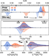 |
Fig. 3 Chemical and isotopic abundance ratios retrieved for Luhman 16AB. Both the results from the free-chemistry and disequilibrium retrievals are shown. For context, we show the abundance ratios of the local ISM (Milam et al. 2005; Wilson 1999) and the Sun (Asplund et al. 2021; Lyons et al. 2018). |
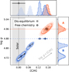 |
Fig. 4 Retrieved correlation between surface gravity and the carbon abundance, relative to hydrogen and the solar value (i.e. [C/H]; Asplund et al. 2021). To a first order, these two parameters follow a linear relation and can be projected onto the expected log gA = 4.96 and log gB = 4.88. |
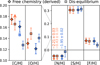 |
Fig. 5 Abundances of carbon, oxygen, nitrogen, sulphur, and fluorine as inferred from the detected gaseous molecules (see Sect. 3.1). The values are shown relative to the solar composition and uncertainties reported by Asplund et al. (2021). |
3.3 Disequilibrium chemistry
At the L-T transition, brown dwarfs can experience vigorous vertical mixing, which upsets their chemical equilibrium (e.g. Hubeny & Burrows 2007; Zahnle & Marley 2014; Mukherjee et al. 2022). In this section, we investigate the severity of disequilibrium in the Luhman 16 atmospheres by employing the FastChem model outlined in Sect. 2.2.3. Figure 6 presents the retrieved temperature and abundance profiles, which are corrected for the surface-gravity degeneracy following Sect. 3.2. The right panels compare the disequilibrium abundances with the vertically constant free-chemistry abundances and shows good agreement between all molecules at the photospheres.
Although most species show similar concentrations across the binary, CH4 and NH3 are distinctly more abundant in Luhman 16B. For L-T transition objects, CH4 is particularly sensitive to the atmospheric dynamics as stronger vertical mixing leads to deeper quenching and thus a lower abundance (Zahnle & Marley 2014; Moses et al. 2016). We find somewhat stronger mixing in Luhman 16A, which reduces the mixing timescale and causes a deeper quenching of CH4 (and NH3) as is illustrated by the middle panel of Fig. 6. The diffusivities - which affect only the chemistry - are constrained at ![Mathematical equation: $\log(K_\mathrm{zz}[\mathrm{cm^2\ s^{-1}}])=8.70^{+0.25}_{-0.21}$](/articles/aa/full_html/2026/03/aa58089-25/aa58089-25-eq18.png) and
and  for Luhman 16A and B, respectively. This corresponds to quenching
  and
and  . The Luhman 16B atmosphere is cooler by ~100 K at these quench points, as evidenced by the left panel of Fig. 6. We hypothesise that the elevated temperature on the primary component may stem from the radiative feedback of more abundant clouds (e.g. Morley et al. 2024). The high mixing strengths in Luhman 16AB align well with the retrieval results for two older L-T transition objects, HD 4747B and DENIS J0255 (Xuan et al. 2022; de Regt et al. 2024).
4 Discussion
4.1 Chemistry across wavelengths
The right panels of Fig. 6 compare the chemical abundance constraints of this work with the measurements of de Regt et al. (2025b), obtained from CRIRES+ J-band spectra. Since the opacity cross-sections depend strongly on the probed wavelength range, we do not cover all molecules and atoms in both bands. Yet, we detect H2O and HF at both wavelengths, for both brown dwarfs, and find equal mixing ratios. As the J band probes deeper into the atmosphere than the K band (~10 vs 1 bar) the stable H2O and HF abundances provide evidence of vertical homogenisation, which is also visible from the chemical disequilibrium profiles in the upper right panel of Fig. 6.
Due to their close proximity to the Earth, Luhman 16A and B are the most studied brown dwarfs with observations that cover a wide range of wavelengths and spectral resolutions. Here, we put our CRIRES+ J- and K-band analyses into context by reviewing the chemical constituents of the Luhman 16 atmospheres. Spectroscopic studies at optical wavelengths commonly find atomic lines from the alkalis Na, K, Rb, and Cs (Luhman 2013; Heinze et al. 2021) as well as Li, which affirms the sub-stellar nature of the binary (Faherty et al. 2014; Lodieu et al. 2015). The bluer near-IR bands (Y, J) still probe Na and K lines, while absorption from the metal hydrides CrH and FeH is also identified in both brown dwarfs (Burgasser et al. 2013, 2014; Faherty et al. 2014; Buenzli et al. 2015b,a; Lodieu et al. 2015; Kellogg et al. 2017). In de Regt et al. (2025b), we present the first abundance constraints of FeH, Na and K (see Fig. 6). Despite the FeH detections at shorter wavelengths, the high-resolution H-band spectra of Ishikawa et al. (2025) do not show the strong FeH band head expected at 1582 nm. Interestingly, this discrepancy may be explained by the rainout of gaseous FeH into iron clouds, which leads to a rapidly decreasing abundance with altitude (Visscher et al. 2010; Burningham et al. 2021; Rowland et al. 2023). Shorter wavelengths generally probe deeper in the atmosphere (e.g. Vos et al. 2023; McCarthy et al. 2025) where the higher temperatures prevent the complete condensation of FeH, while the higher H-band altitudes might be too depleted in FeH to be detectable.
The volatile molecules H2O, CO and CH4 dominate the near-IR spectrum (e.g. Crossfield et al. 2014; Biller et al. 2024; Chen et al. 2024, 2025). While most spectral features are comparable between Luhman 16A and B, CH4 absorption is notably stronger in the T-type component (e.g. Burgasser et al. 2013; Faherty et al. 2014; Lodieu et al. 2015; Kellogg et al. 2017). In this work, we confirm that CH4 is indeed more abundant in the Luhman 16B atmosphere as a result of less efficient vertical mixing. The lower quench pressure also enhances the NH3 abundance, which leads to somewhat deeper absorption in the K band, as noted by Ishikawa et al. (2025). We highlight that the latest high-resolution spectra (R >−104) presented in Ishikawa et al. (2025), de Regt et al. (2025b), and this work have expanded the chemical inventory to include weakly contributing volatiles like NH3, H2S, HF, and 13CO. Ishikawa et al. (2025) also make the first direct measurement of the main atmospheric constituent, H2, using lines at 2121.8, 2223.3, and 2406.6 nm. We cannot reproduce this because the CRIRES+ K2166 setting does not cover these wavelengths. Lastly, recent JWST variability monitoring has expanded the spectroscopic coverage up to 14 μm (Biller et al. 2024; Chen et al. 2025). These JWST spectra access more absorption bands of H2O, CO, and CH4 as well as the 8-11 μm silicate-oxide cloud feature that is weak for Luhman 16A and not detected for B, consistent with the expected clearing of photospheric condensates at the L-T transition (Chen et al. 2025).
 |
Fig. 6 Comparison of temperature and abundance constraints. Left panel : temperature profiles of Luhman 16A and B, retrieved with the chemical disequilibrium model described in Sect. 2.2.3. Luhman 16A displays a heating of ~100 K near the photosphere, which is indicated by the shaded regions in the left side of the panel. Middle panel : mixing and chemical reaction timescales as functions of pressure. The intersection where vertical mixing becomes more efficient than the CO-CH4 reaction is indicated by a horizontal bar. The higher Kzz for Luhman 16A is visible from its reduced mixing timescale. Right panels : cutouts of the chemical abundance profiles between 0.06 and 30 bar. From top to bottom : chemical disequilibrium and free-chemistry abundances from the K-band analysis of this work, and the CRIRES+ J-band constraints presented in de Regt et al. (2025b). The envelopes and error bars in all panels show the 68% credible region. |
4.2 Implications for the formation history
From the disequilibrium retrievals, we constrained bulk ratios of  and
and  , which are consistent with the solar value (0.59 ± 0.08; Asplund et al. 2021). To our knowledge, only one other member of the Oceanus moving group (bona fide or high-likelihood; Gagné et al. 2023), the G5 star HD 77006A, has a reported C/O of 0.51 ± 0.03 (Takeda 2023). This comparison suggests a possible tension between objects that formed in the same environment, but further C/O measurements of Oceanus members are needed to draw such conclusions. Moreover, we note that the inferred bulk C/O ratios depend on the condensation efficiency, for instance through the availability of magnesium and silicon (Calamari et al. 2024) for which we assumed solar abundances in this work. The metallicities in the Oceanus group cluster near the solar value (e.g. [Fe/H] ~ −0.01; Takeda 2023, −0.03 ± 0.03, 0.10 ± 0.09, 0.08 ± 0.05; Soubiran et al. 2022, 0.10 ± 0.18; Hejazi et al. 2022, —0.50; Steinmetz et al. 2020) but there is enough spread that our estimate of [C/H] ~ 0.15 for Luhman 16AB is congruent with the previous studies.
The similar 12C/13C ratios that we find between the binary reinforce the presumed shared formation and evolution history.
In addition to the biases discussed in Sect. 3.1, the co-evolving context gives another reason to question the validity of the discrepant H216O/H218O ratios that are retrieved between A and B. The carbon isotope ratios of Luhman 16AB (12C/13C ~ 74) are in line with the present-day, local ISM (12C/13CISM = 68 ± 15; Milam et al. 2005) but lower than the solar wind (12C/13C⊙ = 93.5 ± 3.1; Lyons et al. 2018). Models of galactic chemical evolution predict an enhancement of the interstellar 13C over time (Romano 2022) and recent observations of M-dwarf stars confirm this trend (González Picos et al. 2025b). The elevated 13C abundance we find for Luhman 16AB is thus compatible with recent inheritance from the ISM, which provides further evidence for the modestly young age of Luhman 16AB (−500 Myr; Gagné et al. 2023).
Since the oxygen isotope is not confidently detected in the presented analysis, we refrain from interpreting the 16O/18O ratios in the context of the Luhman 16AB formation history. The high rotational velocities of Luhman 16AB (v sin i = 14.76 ± 0.03 and 24.79 ± 0.04 km s−1) hinder the identification of C18O and H218O absorption lines as they become blended with neighbouring features. Slower rotators typically present tentative to more credible evidence of minor isotopologues, even in K-band spectra of lower quality compared to those of Luhman 16AB (Zhang et al. 2022; Xuan et al. 2024; González Picos et al. 2024, 2025b; Mulder et al. 2025; Grasser et al. 2025). The strongest CO absorption is found at its fundamental band (4.3-5.1 μm) and can be accessed with high-resolution M-band spectroscopy (Crossfield et al. 2019). Though Luhman 16A and B are bright enough, ground-based observations suffer from the high thermal sky background (Parker et al. 2024). Alternatively, recent medium-resolution JWST spectra (R ~ 3000) have uncovered several minor isotopologues, including 13CO, C18O, C17O (Gandhi et al. 2023; Lew et al. 2024; Mollière et al. 2025; González Picos et al. 2025a), 15NH3 (Barrado et al. 2023; Kühnle et al. 2025), as well as CH3D (Rowland et al. 2024). Given the high brightness, it is reasonable to expect that these isotopologues are also detectable in the Luhman 16AB atmospheres.
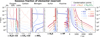 |
Fig. 7 Abundance profiles of gases as a fraction of the total elemental reservoir of oxygen, carbon, nitrogen, sulphur, and fluorine. The abundances are calculated with FastChem Cond (Kitzmann et al. 2024), using SONORA Elf Owl temperature structures (shown in the right panel; Mukherjee et al. 2024) that are representative of Y-, T-, L- and late M-type dwarfs. Oxygen and carbon are carried by multiple gaseous molecules (H2O, CO, and CH4), which are shown as their separate and summed profiles. The condensation points of important cloud species are indicated as arrowheads for reference. |
4.3 Detectable reservoir of elements
Measurements of molecular gases in sub-stellar atmospheres do not always reflect the bulk elemental composition because the chemistry might favour the formation of other, unobserved gases or condensates. Here, we investigate which molecules reliably trace the elemental reservoirs across late M-, L-, T-, and Y-type temperature profiles, obtained from the SONORA Elf Owl modelling suite (Mukherjee et al. 2024). We employed FastChem (Kitzmann et al. 2024) to compute the chemical equilibrium and include the effects of condensation and rainout. The input consists of a proto-solar composition, as tabulated by Bergemann et al. (2026). Combined with the output number densities, we calculated the fraction of oxygen, carbon, nitrogen, sulphur, and fluorine that is carried by selected molecular gases, and this is presented in Fig. 7. As an example, in the hotter (≤ T1) atmospheres NH3 probes ≲−10% of the nitrogen because this element primarily exists in undetectable N2 gas (Lodders & Fegley 2002). This implies that NH3 will underestimate the total nitrogen concentration, as we found from the free-chemistry model in Sect. 3.2. Similarly for higher temperatures, sulphur converts to SH and atomic S gas (Visscher et al. 2006), leading to a decreasing H2S fraction with depth. However, at the Luhman 16AB temperatures H2S is the predominant sulphur carrier, which explains the consistent [S/H] derived for the free-chemistry model and its retrieved value in the equilibrium model, as noted in Sect. 3.2.
The oxygen sequestration outlined in Sect. 3.2 is demonstrated by the gas reduction that is seen at the Mg2SiO4 condensation points (green arrows) in Fig. 7. Above those points, the summed H2O and CO measurements can account for ~80% of the oxygen concentration in the calculated models, but we note that the extent of oxygen-trapping depends on assumptions of the condensation physics such as the availability of magnesium and silicon (Calamari et al. 2024). Below the condensation points, gaseous SiO holds ~6% of the oxygen budget. The Y-dwarf (Teff = 400 K) reveals eventual depletions of nitrogen and oxygen when ammonia and water ices form, respectively (Morley et al. 2014). Fortunately, the carbon reservoir is measured fully by summing the CH4 and CO abundances. For this reason, we recommend the adoption of [C/H] as a proxy for the metallicity when both CO and CH4 can be measured. It should be noted that the FastChem models shown in Fig. 7 do not consider disequilibrium chemistry although that should minimally affect the summed abundances of H2O + CO and CH4 + CO or the general trends observed. While CO2 holds a negligible fraction of carbon and oxygen at the assumed protosolar composition (<0.1%), we observe that its contribution increases up to ~8% for both elements at 100 times the solar metallicity.
Hydrogen-fluoride (HF) has recently been detected in the high-resolution spectra of several M dwarfs (González Picos et al. 2025b), brown dwarfs (González Picos et al. 2024; Mulder et al. 2025; Grasser et al. 2025), and high-mass exoplanets (González Picos et al. 2025c; Zhang et al. 2024). Notably, the molecule appears detectable for a broad range of spectral types, i.e. M0-T0.5. Luhman 16A and B are the first sub-stellar objects where HF is detected at J- and K-band wavelengths (de Regt et al. 2025b; Ishikawa et al. 2025). This observed stability with temperature and pressure can be explained using Fig. 7. For each temperature profile, we find that fluorine primarily exists in the form of gaseous HF. The production of AlF gas temporarily reduces the HF fraction to ~65%, but the subsequent rainout of Al-bearing condensates releases fluorine back to form its hydride. Only the Y-dwarf shows a depletion of HF into gaseous H6F6 at ≲10−2 bar. Observations of the cold ISM also find that HF can account for most of the gas-phase fluorine (Gerin et al. 2016). In view of the stability with cooler temperatures, we predict that HF remains detectable in high-resolution J-band spectra of late T-dwarfs (at ≳1.25 μm). In the K band, however, the strong CH4 absorption (e.g. Cushing et al. 2005) likely masks the HF lines beyond ≳2.3 μm.
Previous studies have suggested that fluorine can bond with lithium to form a considerable amount of LiF, both as a gas Gharib-Nezhad et al. (2021) and a condensate species (Lodders 1999; Lodders & Fegley 2006). The creation of LiF, in addition to other lithium compounds (LiCl, LiOH, and LiH; Gharib-Nezhad et al. 2021), could thus contribute to the observed weakening of the optical Li doublet for T-type dwarfs (Kirkpatrick et al. 2008; Martín et al. 2022). The presented FastChem equilibrium models account for the gas- and condensed phase chemistry of lithium as implemented in Kitzmann et al. (in prep.). Consequently, Fig. 7 shows small depletions of HF (~10%) due to the formation of LiF clouds. Lithium is entirely condensed above these points because it is the rarer element compared to fluorine in the proto-solar composition (A (Li) = 3.39 ± 0.02, A (F) = 4.75 ± 0.09; Bergemann et al. 2026). The expected reduction in the HF mixing ratio is only ~0.03 dex, which is outside of most detection limits, even for the nearest brown dwarfs (see Table C.1). For that reason, it appears that gaseous HF measurements cannot provide meaningful constraints on the depletion of lithium. Since most of the fluorine exists as HF, however, this molecule can still serve as a general tracer of metal enrichment.
5 Conclusions
We analysed high-resolution K-band spectra to infer the chemical properties of the Luhman 16AB atmospheres. The CRIRES+ observations resolve the binary brown dwarfs and can be fitted extremely well using our retrieval framework. The fitted models result in detections of H2O, 12CO, CH4, H2S, NH3, HF, and the 13CO isotopologue. The molecular abundances retrieved using a free-chemistry and disequilibrium modelling approach are consistent with one another. The combined CO and CH4 concentrations reveal an unmistakable chemical disequilibrium in the Luhman 16AB atmospheres, while the stronger CH4 and NH3 absorption of component B can be attributed to less vigorous mixing (Kzz,A ~ 108.7 vs Kzz,B ~ 108.2 cm2 s−1). We reviewed the recent detections of HF in sub-stellar atmospheres using chemical equilibrium models. Most fluorine exists in the form of gaseous HF, and this molecule is stable with temperature and pressure, thereby explaining the detections for M-, L-, and T-type dwarfs in addition to the constant abundances that we infer at different depths of Luhman 16AB.
The abundance constraints allowed us to derive bulk carbon-to-oxygen ratios of  and
and  , in line with the solar composition. The retrieved gaseous C/O ratios are higher since oxygen is partially trapped in the silicateoxide clouds. The 13CO detection reveals isotope ratios of
  and
and  , which are enriched in 13C compared to the Sun. The coincident isotope ratios provide further support for the idea that Luhman 16A and B have the same formation histories. Since evolved stars are predicted to enhance the interstellar 13C over time, and 12C/13C ~ 74 aligns with the present-day ISM, the inferred ratios are compatible with a recent inheritance and therefore corroborate the moderately young age of Luhman 16AB (~500 Myr; Gagné et al. 2023). In line with a recent formation, the elemental abundances of carbon, oxygen, sulphur, and fluorine reveal an overall enrichment of metals compared to the solar composition. The metallicity is measured at [C/H] ~ 0.15, but we caution that this value is degenerate with the assumed surface gravity.
This analysis of Luhman 16AB presents some of the best elemental and isotopic abundance constraints of the ESO SupJup Survey and, broadly, for brown dwarfs. It remains challenging, however, to comprehensively understand the atmospheric chemistries. For instance, future studies could explore the chemical abundances in three (or four) dimensions. At the L-T transition in particular, the coupling between clouds and the temperature profile might result in heterogeneous mixing ratios with altitude, longitude, and latitude (Lee et al. 2024; Teinturier et al. 2026). As the closest known brown dwarfs, Luhman 16A and B are prime targets for such in-depth analyses using both high-resolution and broad-wavelength spectroscopy.
Acknowledgements
We thank the anonymous referee for their constructive feedback. We thank Daniel Kitzmann for sharing the latest input files and his help in including lithium in FastChem. We also thank Jackie Faherty and Johanna Vos for a helpful discussion that motivated this addition. S.d.R. and I.S. acknowledge NWO grant OCENW.M.21.010. Based on observations collected at the European Organisation for Astronomical Research in the Southern Hemisphere under ESO programme(s) 110.23RW.002. This workused the Dutch national e-infrastructure with the support of the SURF Cooperative using grant no. EINF-4556 and EINF-9460. This research has made use of the Astrophysics Data System, funded by NASA under Cooperative Agreement 80NSSC21M00561. Software : Astropy (Astropy Collaboration 2022), corner (Foreman-Mackey 2016), FastChem (Kitzmann et al. 2024), Matplotlib (Hunter 2007), NumPy (Harris et al. 2020), petitRADTRANS (Mollière et al. 2019), PyMultiNest (Feroz et al. 2009; Buchner et al. 2014), SciPy (Virtanen et al. 2020).
References
- Ackerman, A. S., & Marley, M. S. 2001, ApJ, 556, 872 [Google Scholar]
- Al Derzi, A. R., Furtenbacher, T., Tennyson, J., Yurchenko, S. N., & Császár, A. G. 2015, J. Quant. Spec. Radiat. Transf., 161, 117 [NASA ADS] [CrossRef] [Google Scholar]
- Arcos, C., Kanaan, S., Chávez, J., et al. 2018, MNRAS, 474, 5287 [NASA ADS] [CrossRef] [Google Scholar]
- Asplund, M., Amarsi, A. M., & Grevesse, N. 2021, A&A, 653, A141 [NASA ADS] [CrossRef] [EDP Sciences] [Google Scholar]
- Astropy Collaboration (Price-Whelan, A. M., et al.) 2022, ApJ, 935, 167 [NASA ADS] [CrossRef] [Google Scholar]
- Azzam, A. A. A., Tennyson, J., Yurchenko, S. N., & Naumenko, O. V. 2016, MNRAS, 460, 4063 [NASA ADS] [CrossRef] [Google Scholar]
- Barber, R. J., Strange, J. K., Hill, C., et al. 2014, MNRAS, 437, 1828 [CrossRef] [Google Scholar]
- Barrado, D., Mollière, P., Patapis, P., et al. 2023, Nature, 624, 263 [NASA ADS] [CrossRef] [Google Scholar]
- Bate, M. R., Bonnell, I. A., & Bromm, V. 2002, MNRAS, 332, L65 [NASA ADS] [CrossRef] [Google Scholar]
- Bedin, L. R., Dietrich, J., Burgasser, A. J., et al. 2024, Astron. Nachr., 345, e20230158 [NASA ADS] [Google Scholar]
- Bergemann, M., Lodders, K., & Palme, H. 2026, in Encyclopedia of Astrophysics, 2, 387 [Google Scholar]
- Bergin, E. A., Bosman, A., Teague, R., et al. 2024, ApJ, 965, 147 [NASA ADS] [CrossRef] [Google Scholar]
- Biller, B. A., Crossfield, I. J. M., Mancini, L., et al. 2013, ApJ, 778, L10 [Google Scholar]
- Biller, B. A., Vos, J. M., Zhou, Y., et al. 2024, MNRAS, 532, 2207 [NASA ADS] [CrossRef] [Google Scholar]
- Blain, D., Mollière, P., & Nasedkin, E. 2024, The J. Open Source Softw., 9, 7028 [Google Scholar]
- Buchner, J., Georgakakis, A., Nandra, K., et al. 2014, A&A, 564, A125 [NASA ADS] [CrossRef] [EDP Sciences] [Google Scholar]
- Buenzli, E., Marley, M. S., Apai, D., et al. 2015a, ApJ, 812, 163 [Google Scholar]
- Buenzli, E., Saumon, D., Marley, M. S., et al. 2015b, ApJ, 798, 127 [Google Scholar]
- Burgasser, A. J., Sheppard, S. S., & Luhman, K. L. 2013, ApJ, 772, 129 [Google Scholar]
- Burgasser, A. J., Gillon, M., Faherty, J. K., et al. 2014, ApJ, 785, 48 [Google Scholar]
- Burningham, B., Faherty, J. K., Gonzales, E. C., et al. 2021, MNRAS, 506, 1944 [NASA ADS] [CrossRef] [Google Scholar]
- Burrows, A., Sudarsky, D., & Hubeny, I. 2006, ApJ, 640, 1063 [Google Scholar]
- Calamari, E., Faherty, J. K., Visscher, C., et al. 2024, ApJ, 963, 67 [NASA ADS] [CrossRef] [Google Scholar]
- Chabrier, G., Johansen, A., Janson, M., & Rafikov, R. 2014, in Protostars and Planets VI, eds. H. Beuther, R. S. Klessen, C. P. Dullemond, & T. Henning, 619 [Google Scholar]
- Chen, X., Biller, B. A., Vos, J. M., et al. 2024, MNRAS, 533, 3114 [Google Scholar]
- Chen, X., Biller, B. A., Tan, X., et al. 2025, MNRAS, 539, 3758 [Google Scholar]
- Chubb, K. L., Naumenko, O., Keely, S., et al. 2018, J. Quant. Spec. Radiat. Transf., 218, 178 [NASA ADS] [CrossRef] [Google Scholar]
- Coles, P. A., Yurchenko, S. N., & Tennyson, J. 2019, MNRAS, 490, 4638 [CrossRef] [Google Scholar]
- Coxon, J. A., & Hajigeorgiou, P. G. 2015, J. Quant. Spec. Radiat. Transf., 151, 133 [NASA ADS] [CrossRef] [Google Scholar]
- Crossfield, I. J. M., Biller, B., Schlieder, J. E., et al. 2014, Nature, 505, 654 [NASA ADS] [CrossRef] [Google Scholar]
- Crossfield, I. J. M., Lothringer, J. D., Flores, B., et al. 2019, ApJ, 871, L3 [NASA ADS] [CrossRef] [Google Scholar]
- Cushing, M. C., Rayner, J. T., & Vacca, W. D. 2005, ApJ, 623, 1115 [Google Scholar]
- de Regt, S., Gandhi, S., Snellen, I. A. G., et al. 2024, A&A, 688, A116 [NASA ADS] [CrossRef] [EDP Sciences] [Google Scholar]
- de Regt, S., Gandhi, S., Siebenaler, L., & González Picos, D. 2025a, arXiv eprints [arXiv:2510.20870] [Google Scholar]
- de Regt, S., Snellen, I. A. G., Allard, N. F., et al. 2025b, A&A, 696, A225 [NASA ADS] [CrossRef] [EDP Sciences] [Google Scholar]
- Dorn, R. J., Bristow, P., Smoker, J. V., et al. 2023, A&A, 671, A24 [NASA ADS] [CrossRef] [EDP Sciences] [Google Scholar]
- Faherty, J. K., Beletsky, Y., Burgasser, A. J., et al. 2014, ApJ, 790, 90 [NASA ADS] [CrossRef] [Google Scholar]
- Faherty, J. K., Riedel, A. R., Cruz, K. L., et al. 2016, ApJS, 225, 10 [Google Scholar]
- Feroz, F., Hobson, M. P., & Bridges, M. 2009, MNRAS, 398, 1601 [NASA ADS] [CrossRef] [Google Scholar]
- Foreman-Mackey, D. 2016, J. Open Source Softw., 1, 24 [Google Scholar]
- Fuda, N., Apai, D., Nardiello, D., et al. 2024, ApJ, 965, 182 [Google Scholar]
- Gagné, J., Moranta, L., Faherty, J. K., et al. 2023, ApJ, 945, 119 [CrossRef] [Google Scholar]
- Gandhi, S., de Regt, S., Snellen, I., et al. 2023, ApJ, 957, L36 [NASA ADS] [CrossRef] [Google Scholar]
- Geballe, T. R., Saumon, D., Golimowski, D. A., et al. 2009, ApJ, 695, 844 [NASA ADS] [CrossRef] [Google Scholar]
- Gerin, M., Neufeld, D. A., & Goicoechea, J. R. 2016, ARA&A, 54, 181 [Google Scholar]
- Gharib-Nezhad, E., Marley, M. S., Batalha, N. E., et al. 2021, ApJ, 919, 21 [Google Scholar]
- González Picos, D., Snellen, I. A. G., de Regt, S., et al. 2024, A&A, 689, A212 [NASA ADS] [CrossRef] [EDP Sciences] [Google Scholar]
- González Picos, D., de Regt, S., Gandhi, S., Grasser, N., & Snellen, I. A. G. 2025a, A&A, 703, A65 [NASA ADS] [CrossRef] [EDP Sciences] [Google Scholar]
- González Picos, D., Snellen, I., & de Regt, S. 2025b, Nat. Astron., 9, 1692 [Google Scholar]
- González Picos, D., Snellen, I. A. G., de Regt, S., et al. 2025c, A&A, 693, A298 [NASA ADS] [CrossRef] [EDP Sciences] [Google Scholar]
- Grasser, N., Snellen, I. A. G., de Regt, S., et al. 2025, A&A, 698, A252 [NASA ADS] [CrossRef] [EDP Sciences] [Google Scholar]
- Hargreaves, R. J., Gordon, I. E., Huang, X., Toon, G. C., & Rothman, L. S. 2025, J. Quant. Spec. Radiat. Transf., 333, 109324 [Google Scholar]
- Harris, C. R., Millman, K. J., van der Walt, S. J., et al. 2020, Nature, 585, 357 [NASA ADS] [CrossRef] [Google Scholar]
- Harris, G. J., Tennyson, J., Kaminsky, B. M., Pavlenko, Y. V., & Jones, H. R. A. 2006, MNRAS, 367, 400 [Google Scholar]
- Heinze, A. N., Metchev, S., Kurtev, R., & Gillon, M. 2021, ApJ, 920, 108 [Google Scholar]
- Hejazi, N., Lépine, S., & Nordlander, T. 2022, ApJ, 927, 122 [NASA ADS] [CrossRef] [Google Scholar]
- Hoeijmakers, H. J., Seidel, J. V., Pino, L., et al. 2020, A&A, 641, A123 [NASA ADS] [CrossRef] [EDP Sciences] [Google Scholar]
- Hubeny, I., & Burrows, A. 2007, ApJ, 669, 1248 [Google Scholar]
- Hunter, J. D. 2007, Comput. Sci. Eng., 9, 90 [NASA ADS] [CrossRef] [Google Scholar]
- Ishikawa, H. T., Metchev, S., Tannock, M. E., et al. 2025, MNRAS, 539, 1088 [Google Scholar]
- Kellogg, K., Metchev, S., Heinze, A., Gagné, J., & Kurtev, R. 2017, ApJ, 849, 72 [Google Scholar]
- Kirkpatrick, J. D. 2005, ARA&A, 43, 195 [Google Scholar]
- Kirkpatrick, J. D., Cruz, K. L., Barman, T. S., et al. 2008, ApJ, 689, 1295 [NASA ADS] [CrossRef] [Google Scholar]
- Kitzmann, D., Stock, J. W., & Patzer, A. B. C. 2024, MNRAS, 527, 7263 [Google Scholar]
- Kühnle, H., Patapis, P., Mollière, P., et al. 2025, A&A, 695, A224 [NASA ADS] [CrossRef] [EDP Sciences] [Google Scholar]
- Lazorenko, P. F., & Sahlmann, J. 2018, A&A, 618, A111 [NASA ADS] [CrossRef] [EDP Sciences] [Google Scholar]
- Lee, E. K. H., Tan, X., & Tsai, S.-M. 2024, MNRAS, 529, 2686 [NASA ADS] [CrossRef] [Google Scholar]
- Lew, B. W. P., Roellig, T., Batalha, N. E., et al. 2024, AJ, 167, 237 [NASA ADS] [CrossRef] [Google Scholar]
- Li, G., Gordon, I. E., Le Roy, R. J., et al. 2013, J. Quant. Spec. Radiat. Transf., 121, 78 [Google Scholar]
- Li, G., Gordon, I. E., Rothman, L. S., et al. 2015, ApJS, 216, 15 [NASA ADS] [CrossRef] [Google Scholar]
- Lodders, K. 1999, ApJ, 519, 793 [NASA ADS] [CrossRef] [Google Scholar]
- Lodders, K., & Fegley, B. 2002, Icarus, 155, 393 [Google Scholar]
- Lodders, K., & Fegley, B. 2006, Chemistry of Low Mass Substellar Objects, ed. J. W. Mason (Berlin, Heidelberg: Springer Berlin Heidelberg), 1 [Google Scholar]
- Lodieu, N., Zapatero Osorio, M. R., Rebolo, R., et al. 2015, A&A, 581, A73 [NASA ADS] [CrossRef] [EDP Sciences] [Google Scholar]
- Lothringer, J. D., Rustamkulov, Z., Sing, D. K., et al. 2021, ApJ, 914, 12 [CrossRef] [Google Scholar]
- Luhman, K. L. 2013, ApJ, 767, L1 [NASA ADS] [CrossRef] [Google Scholar]
- Lyons, J. R., Gharib-Nezhad, E., & Ayres, T. R. 2018, Nat. Commun., 9, 908 [Google Scholar]
- Madhusudhan, N. 2012, ApJ, 758, 36 [NASA ADS] [CrossRef] [Google Scholar]
- Martín, E. L., Lodieu, N., & del Burgo, C. 2022, MNRAS, 510, 2841 [Google Scholar]
- McCarthy, A. M., Vos, J. M., Muirhead, P. S., et al. 2025, ApJ, 981, L22 [Google Scholar]
- Milam, S. N., Savage, C., Brewster, M. A., Ziurys, L. M., & Wyckoff, S. 2005, ApJ, 634, 1126 [Google Scholar]
- Miles, B. E., Skemer, A. J. I., Morley, C. V., et al. 2020, AJ, 160, 63 [NASA ADS] [CrossRef] [Google Scholar]
- Millar-Blanchaer, M. A., Girard, J. H., Karalidi, T., et al. 2020, ApJ, 894, 42 [NASA ADS] [CrossRef] [Google Scholar]
- Mollière, P., & Snellen, I. A. G. 2019, A&A, 622, A139 [NASA ADS] [CrossRef] [EDP Sciences] [Google Scholar]
- Mollière, P., van Boekel, R., Dullemond, C., Henning, T., & Mordasini, C. 2015, ApJ, 813, 47 [Google Scholar]
- Mollière, P., Wardenier, J. P., van Boekel, R., et al. 2019, A&A, 627, A67 [Google Scholar]
- Mollière, P., Stolker, T., Lacour, S., et al. 2020, A&A, 640, A131 [Google Scholar]
- Mollière, P., Kühnle, H., Matthews, E. C., et al. 2025, A&A, 703, A79 [NASA ADS] [CrossRef] [EDP Sciences] [Google Scholar]
- Morley, C. V., Marley, M. S., Fortney, J. J., et al. 2014, ApJ, 787, 78 [Google Scholar]
- Morley, C. V., Skemer, A. J., Miles, B. E., et al. 2019, ApJ, 882, L29 [NASA ADS] [CrossRef] [Google Scholar]
- Morley, C. V., Mukherjee, S., Marley, M. S., et al. 2024, ApJ, 975, 59 [NASA ADS] [CrossRef] [Google Scholar]
- Moses, J. I., Marley, M. S., Zahnle, K., et al. 2016, ApJ, 829, 66 [Google Scholar]
- Mukherjee, S., Fortney, J. J., Batalha, N. E., et al. 2022, ApJ, 938, 107 [NASA ADS] [CrossRef] [Google Scholar]
- Mukherjee, S., Fortney, J. J., Morley, C. V., et al. 2024, ApJ, 963, 73 [NASA ADS] [CrossRef] [Google Scholar]
- Mulder, W., de Regt, S., Landman, R., et al. 2025, A&A, 694, A164 [NASA ADS] [CrossRef] [EDP Sciences] [Google Scholar]
- Noll, K. S., Geballe, T. R., & Marley, M. S. 1997, ApJ, 489, L87 [NASA ADS] [CrossRef] [Google Scholar]
- Öberg, K. I., & Bergin, E. A. 2021, Phys. Rep., 893, 1 [Google Scholar]
- Öberg, K. I., Murray-Clay, R., & Bergin, E. A. 2011, ApJ, 743, L16 [Google Scholar]
- Parker, L. T., Birkby, J. L., Landman, R., et al. 2024, MNRAS, 531, 2356 [Google Scholar]
- Polyansky, O. L., Kyuberis, A. A., Lodi, L., et al. 2017, MNRAS, 466, 1363 [NASA ADS] [CrossRef] [Google Scholar]
- Polyansky, O. L., Kyuberis, A. A., Zobov, N. F., et al. 2018, MNRAS, 480, 2597 [NASA ADS] [CrossRef] [Google Scholar]
- Radigan, J., Lafrenière, D., Jayawardhana, R., & Artigau, E. 2014, ApJ, 793, 75 [NASA ADS] [CrossRef] [Google Scholar]
- Redfield, S., Endl, M., Cochran, W. D., & Koesterke, L. 2008, ApJ, 673, L87 [Google Scholar]
- Romano, D. 2022, A&A Rev., 30, 7 [Google Scholar]
- Rowland, M. J., Morley, C. V., & Line, M. R. 2023, ApJ, 947, 6 [NASA ADS] [CrossRef] [Google Scholar]
- Rowland, M. J., Morley, C. V., Miles, B. E., et al. 2024, ApJ, 977, L49 [Google Scholar]
- Saumon, D., & Marley, M. S. 2008, ApJ, 689, 1327 [Google Scholar]
- Smette, A., Sana, H., Noll, S., et al. 2015, A&A, 576, A77 [NASA ADS] [CrossRef] [EDP Sciences] [Google Scholar]
- Smith, M. D. 1998, Icarus, 132, 176 [NASA ADS] [CrossRef] [Google Scholar]
- Somogyi, W., Yurchenko, S. N., & Yachmenev, A. 2021, J. Chem. Phys., 155, 214303 [NASA ADS] [CrossRef] [Google Scholar]
- Soubiran, C., Brouillet, N., & Casamiquela, L. 2022, A&A, 663, A4 [NASA ADS] [CrossRef] [EDP Sciences] [Google Scholar]
- Steinmetz, M., Guiglion, G., McMillan, P. J., et al. 2020, AJ, 160, 83 [NASA ADS] [CrossRef] [Google Scholar]
- Takeda, Y. 2023, Res. Astron. Astrophys., 23, 025008 [Google Scholar]
- Teinturier, L., Charnay, B., Spiga, A., & Bézard, B. 2026, Nat. Astron. [arXiv:2510.18090] [Google Scholar]
- Thorngren, D. P., Sing, D. K., & Mukherjee, S. 2025, arXiv e-prints [arXiv:2510.00169] [Google Scholar]
- Tremblin, P., Amundsen, D. S., Chabrier, G., et al. 2016, ApJ, 817, L19 [NASA ADS] [CrossRef] [Google Scholar]
- Turrini, D., Schisano, E., Fonte, S., et al. 2021, ApJ, 909, 40 [Google Scholar]
- Virtanen, P., Gommers, R., Oliphant, T. E., et al. 2020, Nat. Methods, 17, 261 [Google Scholar]
- Visscher, C., Lodders, K., & Fegley, Jr., B. 2006, ApJ, 648, 1181 [NASA ADS] [CrossRef] [Google Scholar]
- Visscher, C., Lodders, K., & Fegley, Jr., B. 2010, ApJ, 716, 1060 [NASA ADS] [CrossRef] [Google Scholar]
- Vos, J. M., Burningham, B., Faherty, J. K., et al. 2023, ApJ, 944, 138 [NASA ADS] [CrossRef] [Google Scholar]
- Wiescher, M., Görres, J., Uberseder, E., Imbriani, G., & Pignatari, M. 2010, Annu. Rev. Nucl. Part. Sci., 60, 381 [Google Scholar]
- Wilson, T. L. 1999, Rep. Progr. Phys., 62, 143 [CrossRef] [Google Scholar]
- Xuan, J. W., Wang, J., Ruffio, J.-B., et al. 2022, ApJ, 937, 54 [NASA ADS] [CrossRef] [Google Scholar]
- Xuan, J. W., Wang, J., Finnerty, L., et al. 2024, ApJ, 962, 10 [NASA ADS] [CrossRef] [Google Scholar]
- Yurchenko, S. N., Owens, A., Kefala, K., & Tennyson, J. 2024, MNRAS, 528, 3719 [CrossRef] [Google Scholar]
- Zahnle, K. J., & Marley, M. S. 2014, ApJ, 797, 41 [CrossRef] [Google Scholar]
- Zhang, Y., Snellen, I. A. G., & Mollière, P. 2021, A&A, 656, A76 [NASA ADS] [CrossRef] [EDP Sciences] [Google Scholar]
- Zhang, Y., Snellen, I. A. G., Brogi, M., & Birkby, J. L. 2022, RNAAS, 6, 194 [NASA ADS] [Google Scholar]
- Zhang, Z., Mollière, P., Hawkins, K., et al. 2023, AJ, 166, 198 [NASA ADS] [CrossRef] [Google Scholar]
- Zhang, Y., González Picos, D., de Regt, S., et al. 2024, AJ, 168, 246 [NASA ADS] [CrossRef] [Google Scholar]
- Zhang, Z., Mollière, P., Fortney, J. J., & Marley, M. S. 2025, AJ, 170, 64 [Google Scholar]
Appendix A Cross-correlation bootstrap validation
As explained in Sect. 3.1, several effects can result in the pseudostochastic CCF structure observed for both brown dwarfs in Fig. 2. Particularly for weak contributors, whose line depths are smaller than some spectral residuals, it is possible that random alignments can result in a 2 to 4σ peak at the expected velocity. To evaluate the detectability of the signal at other velocities, we fitted Gaussian profiles to the H28O and C18O CCFs at vrad = 0 km s−1. As shown in the left panel of Fig. A.1, the fitted peak is subtracted and re-injected at another velocity, where the S /N is evaluated again. Following a bootstrap method (e.g. Redfield et al. 2008; Hoeijmakers et al. 2020), this injection and evaluation is performed between −1000 and +1000 km s−1 in steps of 1 km s−1. The resulting S/N distributions of Luhman 16A and B are presented in Fig. A.1. Since the distributions are not clearly separated from a significance of 0σ, we cannot confidently claim detections of these molecules.
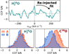 |
Fig. A.1 Bootstrap validation of H218O and C18O cross-correlation signals. Top panel : example of the removal and re-injection of the H218O CCF peak for Luhman 16A. Bottom panels : cross-correlation S/N distributions measured after injections between ±1000 km s−1. |
Appendix B Reduced equilibrium-chemistry model
We created a reduced input for the equilibrium-chemistry code FastChem Cond (Kitzmann et al. 2024) in an effort to shorten computation times to be suitable for usage during a retrieval. Table B.1 shows the included atomic gases, molecular gases, and condensate species. These are chosen based on their prevalence or impact on the gaseous compositions of L- or early T-type brown-dwarf atmospheres. This reduction from 618 gases and 235 condensates in the FastChem extended input down to, respectively, 43 and 16 species accelerates the computation by at least 10 times. Depending on the number of atmospheric layers, temperatures, and CPU clock speed, the reduced input with rainout condensation typically converges in ≲−0.2 s.
Naturally, the reduced model comes at a cost of accuracy compared to the extended FastChem input. Figure B.1 presents the deviations between the reduced (solid) and complete (dashed) reaction networks. The abundance profiles of these molecules minimally differ between the two approaches, especially at ≲−10 bar. We quantified the deviation in log VMRs across all pressures via the root mean square error (RMSE), and present this for each molecule at varying metallicities and C/O ratios in the right panels of Fig. B.1. Apart from the deviation of H2S and HF in the lower atmosphere, the tested compositions yield RMSE <−0.05 dex for the other molecules. We therefore conclude that the reduced equilibrium-chemistry model is sufficiently accurate and can be employed for L-T transition objects with plausible compositions.
Gaseous and condensate species included in our reduced FastChem input, sorted by mass.
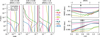 |
Fig. B.1 Accuracy validation of reduced FastChem input compared to the complete, extended equilibrium-chemistry model. Left panels : deviation in VMRs for a solar composition (Asplund et al. 2021), a 10 times solar metallicity, and a C/O = 1.0, assuming a Teff = 1300 K temperature profile (Mukherjee et al. 2024). Right panels : RMSE between the log VMRs of the two inputs at varying metallicities and C/O ratios. |
Appendix C Extended retrieval results
Retrieved parameters and their uncertainties.
Appendix D Best-fitting spectra
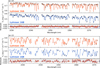 |
Fig. D.2 Continued. |
All Tables
Gaseous and condensate species included in our reduced FastChem input, sorted by mass.
All Figures
|
Fig. 1 CRIRES+ K-band spectra of Luhman 16A and B in orange and blue, respectively. Top panel : seven spectral orders covered in the K2166 wavelength setting. The telluric absorption is shown as transparent lines. Lower panels : zoom-in of the sixth order. The black observed spectra are overlaid with the best-fitting free-chemistry models in orange and blue. The mean scaled uncertainties are displayed to the right of the residuals in the bottom panel. The fits to the other spectral orders can be found in Appendix D. |
| In the text | |
|
Fig. 2 Cross-correlation analysis of minor species in the spectra of Luhman 16A (solid) and B (dashed). The detection significance at v = 0 km s−1 is indicated in the upper-right corner of each panel, with Luhman 16A at the top. The panel rows use different y-axis limits for legibility. |
| In the text | |
|
Fig. 3 Chemical and isotopic abundance ratios retrieved for Luhman 16AB. Both the results from the free-chemistry and disequilibrium retrievals are shown. For context, we show the abundance ratios of the local ISM (Milam et al. 2005; Wilson 1999) and the Sun (Asplund et al. 2021; Lyons et al. 2018). |
| In the text | |
|
Fig. 4 Retrieved correlation between surface gravity and the carbon abundance, relative to hydrogen and the solar value (i.e. [C/H]; Asplund et al. 2021). To a first order, these two parameters follow a linear relation and can be projected onto the expected log gA = 4.96 and log gB = 4.88. |
| In the text | |
|
Fig. 5 Abundances of carbon, oxygen, nitrogen, sulphur, and fluorine as inferred from the detected gaseous molecules (see Sect. 3.1). The values are shown relative to the solar composition and uncertainties reported by Asplund et al. (2021). |
| In the text | |
|
Fig. 6 Comparison of temperature and abundance constraints. Left panel : temperature profiles of Luhman 16A and B, retrieved with the chemical disequilibrium model described in Sect. 2.2.3. Luhman 16A displays a heating of ~100 K near the photosphere, which is indicated by the shaded regions in the left side of the panel. Middle panel : mixing and chemical reaction timescales as functions of pressure. The intersection where vertical mixing becomes more efficient than the CO-CH4 reaction is indicated by a horizontal bar. The higher Kzz for Luhman 16A is visible from its reduced mixing timescale. Right panels : cutouts of the chemical abundance profiles between 0.06 and 30 bar. From top to bottom : chemical disequilibrium and free-chemistry abundances from the K-band analysis of this work, and the CRIRES+ J-band constraints presented in de Regt et al. (2025b). The envelopes and error bars in all panels show the 68% credible region. |
| In the text | |
|
Fig. 7 Abundance profiles of gases as a fraction of the total elemental reservoir of oxygen, carbon, nitrogen, sulphur, and fluorine. The abundances are calculated with FastChem Cond (Kitzmann et al. 2024), using SONORA Elf Owl temperature structures (shown in the right panel; Mukherjee et al. 2024) that are representative of Y-, T-, L- and late M-type dwarfs. Oxygen and carbon are carried by multiple gaseous molecules (H2O, CO, and CH4), which are shown as their separate and summed profiles. The condensation points of important cloud species are indicated as arrowheads for reference. |
| In the text | |
|
Fig. A.1 Bootstrap validation of H218O and C18O cross-correlation signals. Top panel : example of the removal and re-injection of the H218O CCF peak for Luhman 16A. Bottom panels : cross-correlation S/N distributions measured after injections between ±1000 km s−1. |
| In the text | |
|
Fig. B.1 Accuracy validation of reduced FastChem input compared to the complete, extended equilibrium-chemistry model. Left panels : deviation in VMRs for a solar composition (Asplund et al. 2021), a 10 times solar metallicity, and a C/O = 1.0, assuming a Teff = 1300 K temperature profile (Mukherjee et al. 2024). Right panels : RMSE between the log VMRs of the two inputs at varying metallicities and C/O ratios. |
| In the text | |
 |
Fig. D.1 Same as Fig. 1 but showing all spectral orders. |
| In the text | |
|
Fig. D.2 Continued. |
| In the text | |
Current usage metrics show cumulative count of Article Views (full-text article views including HTML views, PDF and ePub downloads, according to the available data) and Abstracts Views on Vision4Press platform.
Data correspond to usage on the plateform after 2015. The current usage metrics is available 48-96 hours after online publication and is updated daily on week days.
Initial download of the metrics may take a while.