| Issue |
A&A
Volume 694, February 2025
|
|
|---|---|---|
| Article Number | A164 | |
| Number of page(s) | 13 | |
| Section | Planets, planetary systems, and small bodies | |
| DOI | https://doi.org/10.1051/0004-6361/202452859 | |
| Published online | 11 February 2025 | |
The ESO SupJup Survey
VI. 12C/13C isotope ratio comparison of three L-type brown dwarfs
1
Leiden Observatory, Leiden University,
Einsteinweg 55,
2333
CC
Leiden,
The Netherlands
2
Department of Astronomy, California Institute of Technology,
Pasadena,
CA
91125,
USA
3
IPAC,
Mail Code 100-22, Caltech, 1200 E. California Boulevard,
Pasadena,
CA
91125,
USA
4
Department of Physics, University of Warwick,
Coventry
CV4 7AL,
UK
5
Centre for Exoplanets and Habitability, University of Warwick,
Gibbet Hill Road,
Coventry
CV4 7AL,
UK
6
School of Natural Sciences, Center for Astronomy, University of Galway,
Galway,
H91 CF50,
Ireland
★ Corresponding author; This email address is being protected from spambots. You need JavaScript enabled to view it.
Received:
4
November
2024
Accepted:
20
January
2025
Abstract
Context. Recent research suggests that the distinct formation processes of exoplanets and brown dwarfs may have an influence on the chemical and isotopic composition of their atmospheres. Variations in the carbon 12C/13C isotope ratio have been observed and tentatively linked to the top-down formation of brown dwarfs and the core accretion pathway of super-Jupiters. The ESO SupJup Survey, conducted with CRIRES+ on the Very Large Telescope, aims to characterise the atmospheres of young brown dwarfs and super-Jupiters, specifically by investigating the 12C/13C ratio as a tracer of their formation pathways.
Aims. We present the atmospheric characterisation of three isolated L-type brown dwarfs (2MASS J08354256-0819237, 2MASS J05012406-0010452, and 2MASS J05002100+0330501) included in the ESO SupJup Survey. We aim to constrain the C/O and 12C/13C ratios, and investigate whether the oxygen 16O/18O isotope ratio can be probed.
Methods. We analysed the CRIRES+ K-band spectra of the three targets using our atmospheric retrieval framework. This framework couples the radiative transfer code petitRADTRANS with the sampling algorithm MultiNest.
Results. We report 12C/13C ratios of 89−11+11 and 117−17+20 for J0835 and J0500 with strong 13CO significance (>6.5σ) and a tentative (3σ) detection of 13CO for J0501, resulting in a carbon isotope ratio of 155−53+56. Only a weak detection of the H218O isotope was found in J0835. The C/O ratios are found to be in the range 0.65 to 0.71 for the three targets, and all exhibit strong detections of HF.
Conclusions. The 12C/13C ratios appear to be higher than that of the interstellar medium.
Key words: planets and satellites: atmospheres
© The Authors 2025
 Open Access article, published by EDP Sciences, under the terms of the Creative Commons Attribution License (https://creativecommons.org/licenses/by/4.0), which permits unrestricted use, distribution, and reproduction in any medium, provided the original work is properly cited.
This article is published in open access under the Subscribe to Open model. This email address is being protected from spambots. You need JavaScript enabled to view it. to support open access publication.
1 Introduction
Spectroscopic observations of exoplanetary atmospheres allow us to trace their chemical compositions and determine their thermal structure and possible cloud properties (Janson et al. 2010; Barman et al. 2011; Currie et al. 2011; Skemer et al. 2012; Oppenheimer et al. 2013). In addition to providing information about their atmospheric conditions, such a characterisation may help in constraining exoplanet formation and evolutionary processes. High-resolution spectroscopy plays an important role in unveiling the intricacies of exoplanet atmospheres, as it unequivocally determines the presence (Brogi et al. 2012; Hoeijmakers et al. 2020) and abundances (Brogi & Line 2019; Line et al. 2021) of molecular and atomic species, as well as atmospheric dynamics (Brogi et al. 2016; Snellen et al. 2014; Schwarz, Henriette et al. 2016).
The chemical composition of planetary atmospheres is believed to be linked to local formation conditions (Mollière et al. 2022). The chemical abundance ratios may deviate from that of the interstellar medium (ISM) and are governed by the material (gas or ice) they accrete from their environment during formation. As a result, various chemical abundance ratios have been suggested as tracers of planet formation. One planet formation tracer that is commonly studied is the carbon-to-oxygen (C/O) ratio (Oberg et al. 2011; Madhusudhan et al. 2010; Madhusudhan 2012). The local C/O ratio in a protoplanetary disk is likely affected by various snow lines (Piso et al. 2015), namely of H2O, CO, and CO2, which determine whether these molecular species are generally present as ices or in the gas phase. This will subsequently influence the chemical buildup of the planets that form. Other chemical abundance ratios that have been suggested as formation and evolution tracers are, for example, the nitrogen-to-oxygen (N/O) or nitrogen-to-carbon ratio (N/C) for hot Jupiters (Cridland et al. 2016) and gas giants (Turrini et al. 2021), as well as the refractory-to-volatile ratio for ultra-hot Jupiters (Lothringer et al. 2021).
Isotope ratios have also been proposed as potential tracers of planetary formation history and evolution (Clayton & Nittler 2004; Mollière et al. 2019; Zhang et al. 2021b). The deuterium-to-hydrogen (D/H) ratio in our Solar System is of importance for our understanding of the origin and evolution of water within our celestial neighbourhood. In contrast to D/H ratios, the carbon isotope ratio is roughly constant (~89) in the Solar System (Woods & Willacy 2009); however, it varies on galactic scales as 13C is produced within stars that enrich the ISM over time. The current local ISM has an average isotopologue ratio of 68 ± 15 (Langer & Penzias 1993; Milam et al. 2005), significantly lower than that of the Solar System. Interestingly, isotope fractionation processes create variations on protoplanetary disk scales (Woods & Willacy 2009), which could be passed on to exoplanet atmospheres. (Zhang et al. 2021a; Mollière et al. 2019; Line et al. 2021; Bergin et al. 2024).
Young brown dwarfs (BDs) closely resemble super-Jupiters (SJs) in terms of atmospheric characteristics, but are significantly more observationally accessible. This makes them highly valuable for spectroscopic studies. Formed with high temperatures and inflated radii, these self-luminous objects subsequently cool and undergo gravitational contraction, meaning that they are particularly amenable to detailed spectroscopic observations at a young age. Recent advancements in atmospheric retrieval techniques enable the quantitative characterisation of both young BDs and SJs, taking advantage of instruments such as the upgraded Cross-dispersed hIgh-Resolution Infrared Spectrograph (CRIRES+; Dorn et al. 2023) and the Keck Planet Imager and Characterizer (KPIC; Delorme et al. 2021; Wang et al. 2021; Xuan et al. 2022), along with space-based facilities such as the James Webb Space Telescope (JWST; Gandhi et al. 2023).
(Isolated) BDs are believed to form similarly to stars, through the collapse of molecular clouds (Bate et al. 2002; Whitworth et al. 2007), while giant planets such as SJs can follow distinct formation pathways that involve solid and gas accretion (Pollack et al. 1996; Helled et al. 2014). Reliable measurements of chemical abundance (C/O) and isotopic (12C/13C) ratios in representative samples of BDs and SJs could provide crucial insights into these formation processes.
This paper is organised as follows. In Sect. 2 we summarise the main characteristics of our sample of BDs taken from literature. Section 3 addresses the CRIRES+ observations of the BD sample and the corresponding data reduction. Section 4 discusses our forward modelling and the atmospheric retrieval framework. In Sect. 5 the main results of the retrievals are reported, and we discuss the implications of our findings in the context of young BDs and recent literature on C/O and isotope ratios. Finally, Sect. 6 summarises our conclusions.
2 Sample selection
In this work we present high-resolution spectra of three isolated L-type BDs: 2MASS J08354256-0819237, 2MASS J05012406-0010452, and 2MASS J05002100+0330501. These objects were selected from the ESO SupJup Survey (programme ID 1110.C4264, PI: Snellen), which aims to compare the atmospheres of sub-stellar companions and isolated BDs (de Regt et al. 2024; González Picos et al. 2024). The complete sample consists of 49 targets, ranging from early M-type stars to cool T-dwarfs (see Fig. 1). Ultimately, we aim to run retrievals for all objects in the sample.
The three BDs selected for this study have similar spectral types (L4.0-5.0) and effective temperatures (Teff = 1700–1800 K), which allows a comparison between atmospheres at comparable conditions. As a result, differences in the atmospheric chemistry between the BDs could possibly inform us of distinct formation scenarios. In addition, the presented constraints for these isolated BDs can serve for comparison with planetary-mass companions in a similar temperature regime (Zhang et al. 2021b; Zhang et al. 2021a). The probed effective temperatures are typical for sub-stellar L-type objects (Teff = 1300–2200 K, Filippazzo et al. 2015) and allow the formation of mineral and metal condensate clouds in their atmospheres (Tsuji et al. 1996; Visscher et al. 2010). We refer to Table 1 for more detailed properties of the studied BDs.
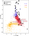 |
Fig. 1 Colour-magnitude diagram of MJ vs J − K showing the observed low- and planetary-mass objects of the ESO SupJup Survey. The companions and their hosts are pictured as black hexagons and diamonds, respectively. All 19 observed isolated BDs are marked as black-outlined circles, and the colour denotes their spectral type. The same colour coding is used for the population of isolated cool dwarfs indicated in the background. These objects, originating from the UltracoolSheet (Best et al. 2024), are shown as a reference. |
2.1 J0835
2MASS J08354256-0819237 (J0835 hereafter) is an isolated L-type BD. Its spectral type, based on photometry, is L5.0 Cruz et al. (2003); Burgasser et al. (2010); Andrei et al. (2011). Previous work used various methods to estimate the effective temperature of J0835, reporting 2200 K (Blake et al. 2010), 1800 ± 100 K (Gagné et al. 2015), 1754 ± 112 K (Filippazzo et al. 2015; Schlawin et al. 2017) and 1374 ± 52 K (Sanghi et al. 2023). Blake et al. (2010) based their Teff on a best-fit synthetic template with log g = 5.0, Gagné et al. (2015) fitted a model using WISE W1 and W2 photometry as well as near-infrared (NIR) spectra in the J, H, and K bands, Filippazzo et al. (2015) used the bolometric luminosity, and Sanghi et al. (2023) combined their own observations and evolutionary model-derived radii to determine semi-empirical effective temperatures.
Gagné et al. (2015) reported no clear signatures of low surface gravity. They determined a surface gravity of log g = 5.0 ± 0.5 using optically anchored NIR spectral average templates. Subsequently, Filippazzo et al. (2015) noted a similar surface gravity of log gJ0835 = 5.19 ± 0.21. In general, low surface gravity BDs are thought to be younger objects with inflated radii, which has been confirmed in previous work (e.g. Kirkpatrick et al. 2008; Liu et al. 2016; Schlawin et al. 2017). Young BDs stand out because of their redder NIR and mid-infrared (MIR) colours and fainter absolute magnitude in the K band when compared to their older spectral counterparts with higher field surface gravities (Gagné et al. 2015; Filippazzo et al. 2015). Liu et al. (2016) describes that J0835 appears to be redder than the bulk of low gravity BDs in the colour-magnitude diagram. They used the gravity-sensitive features (e.g. FeH, Na I, K I, and the H-band continuum shape) in its NIR SpeX prism spectrum (Burgasser et al. 2010) to classify J0835 as on the border between intermediate and field gravity. Their gravity classifications correspond to ages of, respectively, ~30–200 Myr and ~200 Myr. Sanghi et al. (2023) noted a lower surface gravity of log g = 4.32 ± 0.24, which may be related to their significantly different estimate of Teff.
The narrow CO features in the NIRSpec spectra of Blake et al. (2010) are indicative of it being a slow rotator (<20 km s−1). They forward-modelled the extracted spectra and found a rotational velocity of v sin i = 4.18 ± 0.43 km s−1. With those values, Schlawin et al. (2017) provided an estimation of the inclination angle i of 21° (close to pole-on) from photometric variability monitoring, assuming a radius of 1 Jupiter radius.
L dwarfs often exhibit low-level, rotationally modulated photometric variability generally associated with heterogeneous, cloud-covered atmospheres. High-precision ground-based NIR spectrophotometry revealed its spectral variability, likely to be induced by the rapid 3.1 h rotation Koen et al. (2004). In contrast, Schlawin et al. (2017) observed a variability of less than 0.5% per band, with no clear spectral dependence, which is less variability than reported in previous work (Koen et al. 2004; Wilson et al. 2014). They use it to provide an estimation of the inclination angle i of 21° (close to pole-on), assuming a radius of 1 Jupiter radius.
Properties of our L-type BD sample.
2.2 J0501
2MASS J05012406-0010452, hereafter referred to as J0501, is a BD located in the constellation Orion (Reid et al. 2008). Cruz et al. (2009) classifies J0501 as a spectral type L4γ in the optical regime, after which both Liu et al. (2016) and Faherty et al. (2016) classify it as a young field object. Cruz et al. (2009) noted its unusual spectral features, such as notably weak FeH molecular absorption and weak Na I and K I doublets. From this, they concluded the object should have a low surface gravity and is likely a young, low-mass BD. Zapatero Osorio et al. (2014) estimated its effective temperature to be 1720 ± 55 K. Gagné et al. (2015) categorised J0501 in the IR as spectral type L3γ, providing evidence that J0501 is a member of the Columba or Carina moving group (coeval at 20–40 Myr). In this case, the mass is estimated to be, ![Mathematical equation: $\[10.2_{-1.0}^{+0.8}\]$](/articles/aa/full_html/2025/02/aa52859-24/aa52859-24-eq8.png) MJup giving rise to a surface gravity of log g = 4.0 ± 0.5. Vos et al. (2020) measured a rotational velocity of v sin i =
MJup giving rise to a surface gravity of log g = 4.0 ± 0.5. Vos et al. (2020) measured a rotational velocity of v sin i = ![Mathematical equation: $\[9.57_{-0.58}^{+0.67}\]$](/articles/aa/full_html/2025/02/aa52859-24/aa52859-24-eq9.png) km s−1, which in combination with a radius estimate (Filippazzo et al. 2015) results in a maximum rotation period of 15.7 ± 0.2 h.
km s−1, which in combination with a radius estimate (Filippazzo et al. 2015) results in a maximum rotation period of 15.7 ± 0.2 h.
2.3 J0500
2MASS J05002100 +0330501, from hereon referred to as J0500, is a BD at a distance of 13.23 ± 0.05 pc (Gaia Collaboration 2020). Just like J0501, it is also located in the constellation Orion and part of the same moving group. Reid et al. (2008) characterise this BD as a spectral type L4. Filippazzo et al. (2015) estimated an effective temperature of 1793 ± 72 K and a surface gravity of log g = 5.2 ± 0.19 based on its bolometric luminosity. In addition, they derive a mass of 64 ± 14 MJup and a radius of 1.00 ± 0.08 RJup. Burningham et al. (2017) also estimated its effective temperature and surface gravity. They applied a spectral inversion technique in the cloudy L dwarf regime to obtain a temperature estimate of ![Mathematical equation: $\[1796_{-25}^{+23}\]$](/articles/aa/full_html/2025/02/aa52859-24/aa52859-24-eq10.png) K, a surface gravity of, log g =
K, a surface gravity of, log g = ![Mathematical equation: $\[5.21_{-0.08}^{+0.05}\]$](/articles/aa/full_html/2025/02/aa52859-24/aa52859-24-eq11.png) together with H2O, CO, TiO, VO, CaH, CrH, FeH, Na, and K abundances. In comparison to thermochemical equilibrium abundances, they found that the CO and alkali abundances are a factor of ~10 higher and ~2 lower, respectively.
together with H2O, CO, TiO, VO, CaH, CrH, FeH, Na, and K abundances. In comparison to thermochemical equilibrium abundances, they found that the CO and alkali abundances are a factor of ~10 higher and ~2 lower, respectively.
3 Observations and data reduction
3.1 Observations
The observations of J0835, J0501 and J0500, on January 2, February 2 and 28, 2023, respectively, were conducted as part of the SupJup Survey utilising CRIRES+ at the Very Large Telescope (VLT). CRIRES+ (Kaeufl et al. 2004; Dorn et al. 2014, 2023) is an advanced slit spectrograph with adaptive optics capabilities (Paufique et al. 2004), providing high resolution and able to target a broad wavelength range from 0.95 to 5.3 microns with a resolving power of up to R ~ 100 000. Our observations employed the K2166 wavelength setting (1.90–2.48 μm), focusing on regions featuring prominent 12CO and 13CO absorption lines. By utilising the wide slit mode, 0.4″, a spectral resolution of R ~ 64 000, ~56 000, and ~58 000 was obtained for the J0835, J0501, and J0500 observations, respectively (values calculated as described in Appendix A of González Picos et al. 2024). We were not able to use the adaptive optics system as the target BDs are too faint in the R band used for wavefront sensing. Our observation sequence followed an ABBA nodding pattern, of 18, 12, and 4 individual exposures of 300 seconds for J0835, J0501, and J0500, respectively (see Table 2 for a complete overview of the observation parameters).
3.2 Data reduction
The data processing was conducted using the open-source package excalibuhr (Zhang et al. 2024). This involved various corrections including dark-subtraction, flat-fielding, bad-pixel masking and removal of sky emission via AB (or BA) pair subtraction. A and B nodding position frames were mean-combined to produce master frames. After slit curvature and tilt adjustments, the optimal extraction algorithm (Horne 1986) was applied to convert calibrated images into one-dimensional spectra. Telluric standard stars (see Table 2), observed with the same slit- and wavelength settings as the target observations and at similar airmasses, underwent the same reduction procedure.
Atmospheric corrections were performed using Molecfit (Smette et al. 2015). The standard star observations were used to fit the telluric model, which were subsequently scaled to the airmass and precipitable water vapour of the target observation (see González Picos et al. 2024). Detector pixels with telluric transmission of <70% were masked in the observed spectra since they cannot be adequately corrected. The bluest of the seven spectral orders is heavily contaminated with tellurics and therefore not included in our analysis. In addition, the Molecfit model provides a secondary wavelength correction. Finally, the telluriccorrected spectra were flux-calibrated using a simple scaling factor derived from integrated flux measurements in the 2MASS Ks filter-curve and photometry data (Table 2).
Observational parameters for the three L-type BDs.
4 Atmospheric modelling
We adopted a similar atmospheric retrieval framework as used in de Regt et al. (2024). We refer to their work for an elaborate description of the algorithm, likelihood and correlated noise. In this section we summarise the main principles.
4.1 Retrieval framework
The atmospheric retrieval framework is based on the radiative transfer code petitRADTRANS (pRT; Mollière et al. 2019), which computes emission spectra using descriptions of the atmospheric chemistry, cloud structure, surface gravity, and molecular or atomic opacities. pRT was integrated with the nested sampling tool PyMultiNest (Buchner et al. 2014), a Python interface for the MultiNest (Feroz et al. 2019) algorithm. All computations were executed in parallel on the Dutch National Supercomputer Snellius.
The model atmosphere was subdivided into a series of 50 layers covering the atmospheric vertical extent using a pressure range of P = 102−10−5 bar. Each layer was characterised by a temperature and mass fractions of relevant chemical species. The radiative transfer equation was solved for each layer to obtain the flux as a function of wavelength.
Our models accounted for collision-induced absorption (Borysow et al. 1988) from H2-H2 and H2-He (Dalgarno & Williams 1962; Chan & Dalgarno 1965; Gray 2008), as well as Rayleigh scattering of H2 and He. H2O (or ![Mathematical equation: $\[\mathrm{H}_{2}^{16} \mathrm{O}\]$](/articles/aa/full_html/2025/02/aa52859-24/aa52859-24-eq12.png) ), 12CO, 13CO, hydrogen fluoride (HF), Ca and heavy-oxygen water (
), 12CO, 13CO, hydrogen fluoride (HF), Ca and heavy-oxygen water (![Mathematical equation: $\[\mathrm{H}_{2}^{18} \mathrm{O}\]$](/articles/aa/full_html/2025/02/aa52859-24/aa52859-24-eq13.png) ) were included as line opacities. We used ExoMol line lists for the opacities of heavy-oxygen water (
) were included as line opacities. We used ExoMol line lists for the opacities of heavy-oxygen water (![Mathematical equation: $\[\mathrm{H}_{2}^{18} \mathrm{O}\]$](/articles/aa/full_html/2025/02/aa52859-24/aa52859-24-eq14.png) ; Polyansky et al. 2017) and
; Polyansky et al. 2017) and ![Mathematical equation: $\[\mathrm{H}_{2}^{16} \mathrm{O}\]$](/articles/aa/full_html/2025/02/aa52859-24/aa52859-24-eq15.png) (Polyansky et al. 2018). The HITEMP (Rothman et al. 2010) line lists were employed for 12CO, 13CO (Li et al. 2015). Moreover, opacity from HF (Li et al. 2013; Coxon & Hajigeorgiou 2024; Somogyi et al. 2021) was included as a line species following the detection of HF in the atmosphere of two young BDs (González Picos et al. 2024) and in YSES 1b (Zhang et al. 2024). Atomic opacity was included for Ca (Castelli & Kurucz 2003) and several other atoms were evaluated, but not included in the final model. Furthermore, no clouds were included in the atmospheric models (see Sect. 4.3, for more details).
(Polyansky et al. 2018). The HITEMP (Rothman et al. 2010) line lists were employed for 12CO, 13CO (Li et al. 2015). Moreover, opacity from HF (Li et al. 2013; Coxon & Hajigeorgiou 2024; Somogyi et al. 2021) was included as a line species following the detection of HF in the atmosphere of two young BDs (González Picos et al. 2024) and in YSES 1b (Zhang et al. 2024). Atomic opacity was included for Ca (Castelli & Kurucz 2003) and several other atoms were evaluated, but not included in the final model. Furthermore, no clouds were included in the atmospheric models (see Sect. 4.3, for more details).
The pRT model spectra were Doppler-shifted to probe the object’s radial velocity (vrad) and subsequently convolved with a rotational broadening kernel using the fastRotBroad routine (Gray 2008) of PyAstronomy1 (Czesla et al. 2019). The routine applies the projected rotational velocity (v sin i) while taking into account the effects of limb-darkening, fitted with a linear limb-darkening coefficient (εlimb). We implemented instrumental broadening, introduced by the slit spectrograph, by convolving the rotationally broadened spectra with a Gaussian kernel. The width of this kernel corresponds to the R ~ 50.000 spectral resolution of the CRIRES+ instrument. Lastly, the spectra are resampled to the observed wavelength grid for direct comparison with the data.
Generating the significant number of pRT model spectra needed for a statistically supported retrieval is time expensive. The computations of the pRT spectra were sped up by undersampling the high-resolution (λ/Δλ = 106) line-by-line opacities (lbl_opacity_sampling= 3, i.e. R ~ 106/3). The work, done by de Regt et al. (2024) and González Picos et al. (2024), demonstrates that this degree of undersampling is appropriate given the CRIRES+ spectral resolution.
The sampling tool PyMultiNest builds up posterior distributions by sampling the parameter-space of the 18 free parameters and evaluating the likelihood function between the observed and pRT spectra, while obtaining Bayesian evidence (Z) estimates simultaneously. This is an efficient method for exploring and sampling from complex, high-dimensional parameter spaces. A constant sampling efficiency of 5% was used in the importance nested sampling mode. Following Feroz et al. (2019), González Picos et al. (2024), and de Regt et al. (2024), we used 400 live points and an evidence tolerance of 0.5 to sample the posterior distributions. The priors of the retrieved parameters can be found in Table 3.
4.2 Likelihood and correlated noise
We adopted the same likelihood function as used in Landman et al. (2024), González Picos et al. (2024), and de Regt et al. (2024), which is based on the formalism defined by Ruffio et al. (2019). For 18 order-detector pairs (6 spectral orders covered by 3 detectors each), the log-likelihood (ln ℒ) is calculated as
![Mathematical equation: $\[\ln~ \mathcal{L}=-\frac{1}{2}\left(N ~\ln (2 \pi)+~\ln \left(\left|\boldsymbol{\Sigma}_{0}\right|\right)+N ~\ln \left(s^{2}\right)+\frac{1}{s^{2}} \boldsymbol{R}^{T} \boldsymbol{\Sigma}_{0}^{-1} \boldsymbol{R}\right),\]$](/articles/aa/full_html/2025/02/aa52859-24/aa52859-24-eq16.png) (1)
(1)
where N is the number of unmasked pixels (2048 at most), s is the uncertainty scaling factor for the total covariance matrix Σ0 and R = d ϕm represents the residuals between the observed (d) and model (m) spectra for each order-detector pair. The optimal solution for the flux-scaling parameter ![Mathematical equation: $\[\tilde{\phi}\]$](/articles/aa/full_html/2025/02/aa52859-24/aa52859-24-eq98.png) and the optimally scaled residuals
and the optimally scaled residuals ![Mathematical equation: $\[\tilde{s}^{2}\]$](/articles/aa/full_html/2025/02/aa52859-24/aa52859-24-eq99.png) , are found by calculating
, are found by calculating
![Mathematical equation: $\[\tilde{\phi}=\left(\boldsymbol{m}^{T} \Sigma_{0}^{-1} \boldsymbol{m}\right)^{-1} \boldsymbol{m}^{T} \Sigma_{0}^{-1} \boldsymbol{d}, \qquad \text{and} \quad \tilde{s}^{2}=\left.\frac{1}{N} \boldsymbol{R}^{T} \boldsymbol{\Sigma}_{0}^{-1} \boldsymbol{R}\right|_{\phi=\bar{\phi}}.\]$](/articles/aa/full_html/2025/02/aa52859-24/aa52859-24-eq100.png) (2)
(2)
de Regt et al. (2024) highlighted the importance of accounting for correlated noise in CRIRES+ spectra when retrieving model parameter solutions. Using Gaussian processes (GPs), we made sure to model the correlated noise (Kawahara et al. 2022), and address the problem of biases in the retrieved parameters and underestimation of their uncertainties. The covariance of pixels i and j are calculated by adding a diagonal, uncorrelated variance term and an off-diagonal correlated uncertainty term to achieve
![Mathematical equation: $\[\Sigma_{0, i j}=\delta_{i j} \sigma_{i}^{2}+a^{2} \sigma_{\text {eff }, i j}^{2} \exp \left(-\frac{r_{i j}^{2}}{2 \ell^{2}}\right).\]$](/articles/aa/full_html/2025/02/aa52859-24/aa52859-24-eq101.png) (3)
(3)
In Eq. (3), δij is the Kronecker delta function, σi the flux uncertainty of pixel i, σeff,ij the effective uncertainty derived from the data arithmetic mean of the variances of pixels i and j, rij the wavelength separation between pixels, and a and ℓ the GP amplitude and length scale, respectively. The GP amplitude and length scale are retrieved as free parameters.
Retrieved best-fit parameters and their 1σ uncertainty intervals.
4.3 Pressure–temperature profile
In general, BDs are self-luminous objects devoid of significant external irradiation. In the atmosphere, where convection dominates, the atmospheres are expected to have a pres-sure-temperature (P–T) profile in an adiabatic form (Baraffe et al. 2002; Ludwig et al. 2006; Freytag et al. 2010), which implies that both the atmospheric pressure and temperature increase with the atmospheric depth.
The atmospheres were modelled using a similar parameterisation as presented in Zhang et al. (2023). The temperature was parametrised as a function of pressure using values for the temperature gradient ![Mathematical equation: $\[\nabla T_{i} \equiv \frac{\operatorname{dln} T_{i}}{\operatorname{dln}P_{i}}\]$](/articles/aa/full_html/2025/02/aa52859-24/aa52859-24-eq102.png) , where, i corresponds to the number of pressure knots in log-space. In this work, we used five pressure knots where the higher and lower knots are fixed (P1 = 102 and P5 = 10−5). The three intermediate knots were allowed to shift their values. This approach prevented a biased location of the photosphere (see González Picos et al. 2024).
, where, i corresponds to the number of pressure knots in log-space. In this work, we used five pressure knots where the higher and lower knots are fixed (P1 = 102 and P5 = 10−5). The three intermediate knots were allowed to shift their values. This approach prevented a biased location of the photosphere (see González Picos et al. 2024).
The temperature gradients, ∇Tj, of each atmospheric layer were calculated using linear interpolation of the temperatures associated with the pressure knots. Thereafter, the temperatures of each layer were determined using
![Mathematical equation: $\[T_{j}=T_{j-1}\left(\frac{P_{j}}{P_{j-1}}\right)^{\nabla T_{j}}.\]$](/articles/aa/full_html/2025/02/aa52859-24/aa52859-24-eq103.png) (4)
(4)
The central knot (i = 3) was set to be an anchor point for the temperature. As a result, for each model, we retrieved five temperature gradients, three pressure points, and the temperature at the central knot.
We investigated the presence of clouds in the atmospheres of our targets. We made no assumptions regarding cloud composition, and we parameterised the clouds using a ‘grey’ continuum opacity applied at all wavelength. Clouds are likely to have an effect on the strength of the overall continuum and the shape of the temperature profile. No evidence of the presence of clouds was found and therefore clouds were excluded from the final retrieval analyses. This does not mean that these are cloudless objects. They may be present below the K-band photosphere, or equally modelled with a more isothermal P-T profile with similar values for Teff, log g and chemical abundances (Mollière et al. 2020; Zhang et al. 2023). Various retrieval studies of high-resolution K-band spectra resulted in cloud-free solutions as well (e.g. Zhang et al. 2021b; Landman et al. 2024), where Landman et al. (2024) compared models with various and without clouds revealing a consistent C/O abundance ratio. Combining the K-band observations with short-wavelength observations (e.g. Y- or J-band), combining extensive BD photometry measurements with a wider wavelength range, or using the silicate features around 8–10μm (Miles et al. 2023), may further constrain the cloud properties (de Regt et al. 2024).
4.4 Chemical composition
A free-chemistry approach (de Regt et al. 2024) was adopted in which the mixing ratios of line species were treated as independent parameters. This method, also referred to as the free composition (FC) method, includes vertically constant abundances of relevant chemical species while not enforcing any constraints on the relative abundances. The He abundance is held constant at nHe = 0.15 and the H2 abundance is adjusted to obtain a total ntot equal to unity. The constant-with-altitude mixing ratios are expected to be valid for most scenarios for our K-band spectra, as only a limited vertical extent of the BD atmospheres is probed.
The C/O ratios are determined using the chemical abundances of carbon nC and oxygen nO bearing species, according to
![Mathematical equation: $\[\mathrm{C} / \mathrm{O}=\frac{n_{^{12} \mathrm{CO}}+n_{^{13} \mathrm{CO}}}{n_{\mathrm{H}_{2} \mathrm{O}}+{n_{^{12} \mathrm{CO}}+n_{^{13} \mathrm{CO}}}}.\]$](/articles/aa/full_html/2025/02/aa52859-24/aa52859-24-eq104.png) (5)
(5)
The C/O ratio is constant, due to the constant-with-altitude mixing ratios.
The carbon abundance relative to hydrogen is used as a measurement of metallicity:
![Mathematical equation: $\[[\mathrm{C} / \mathrm{H}]=\log _{10}\left(\frac{n_{\mathrm{C}}}{n_{\mathrm{H}}}\right)-\log _{10}\left(\frac{n_{\mathrm{C}}}{n_{\mathrm{H}}}\right)_{\odot},\]$](/articles/aa/full_html/2025/02/aa52859-24/aa52859-24-eq105.png) (6)
(6)
where the solar value is ![Mathematical equation: $\[\log _{10}\left(\frac{n_{\mathrm{C}}}{n_{\mathrm{H}}}\right)_{\odot}=-3.54 \pm 0.04\]$](/articles/aa/full_html/2025/02/aa52859-24/aa52859-24-eq106.png) (Asplund et al. (2021). In a similar manner, the fluorine abundance from HF is calculated through
(Asplund et al. (2021). In a similar manner, the fluorine abundance from HF is calculated through
![Mathematical equation: $\[[\mathrm{F} / \mathrm{H}]=\log _{10}\left(\frac{n_{\mathrm{HF}}}{n_{\mathrm{H}}}\right)-\log _{10}\left(\frac{n_{\mathrm{HF}}}{n_{\mathrm{H}}}\right)_{\odot},\]$](/articles/aa/full_html/2025/02/aa52859-24/aa52859-24-eq107.png) (7)
(7)
where the solar value is ![Mathematical equation: $\[\log _{10}\left(\frac{n_{\mathrm{F}}}{n_{\mathrm{H}}}\right)_{\odot}=-7.6 \pm 0.25\]$](/articles/aa/full_html/2025/02/aa52859-24/aa52859-24-eq108.png) (Asplund et al. (2021).
(Asplund et al. (2021).
We independently retrieved the number fractions of 12CO, 13CO, ![Mathematical equation: $\[\mathrm{H}_{2}^{16} \mathrm{O}\]$](/articles/aa/full_html/2025/02/aa52859-24/aa52859-24-eq109.png) , and
, and ![Mathematical equation: $\[\mathrm{H}_{2}^{18} \mathrm{O}\]$](/articles/aa/full_html/2025/02/aa52859-24/aa52859-24-eq110.png) to determine the carbon and oxygen isotopologue ratios (12C/13C and 16O/18O, respectively) of our BD sample. We want to compare our values of the retrieved carbon and oxygen isotope ratios with those of González Picos et al. (2024). We calculated these ratios using
to determine the carbon and oxygen isotopologue ratios (12C/13C and 16O/18O, respectively) of our BD sample. We want to compare our values of the retrieved carbon and oxygen isotope ratios with those of González Picos et al. (2024). We calculated these ratios using
![Mathematical equation: $\[^{12} \mathrm{C} /^{13} \mathrm{C}=\frac{n_{^{12} \mathrm{CO}}}{n_{^{13} \mathrm{CO}}}; \quad^{16} \mathrm{O} /^{18} \mathrm{O}=\frac{n_{\mathrm{H}_{2}^{16} \mathrm{O}}}{n_{\mathrm{H}_{2}^{18} \mathrm{O}}}.\]$](/articles/aa/full_html/2025/02/aa52859-24/aa52859-24-eq111.png) (8)
(8)
To ensure the reliability of detecting molecular species, we employ a cross-correlation analysis, as detailed in Zhang et al. (2021a). The cross-correlation function (CCF) for each species, X, is computed as follows:
![Mathematical equation: $\[\operatorname{CCF}_{X}(v)=\sum_{i=1}^{N_{\lambda}} \frac{\left(d_{i}-m_{i, \bar{X}}\right)\left(m_{i}-m_{i, \bar{X}}\right)}{\sigma_{i}^{2}},\]$](/articles/aa/full_html/2025/02/aa52859-24/aa52859-24-eq112.png) (9)
(9)
where ![Mathematical equation: $\[m_{i, \bar{X}}\]$](/articles/aa/full_html/2025/02/aa52859-24/aa52859-24-eq113.png) is the atmospheric model without the species X, and mi is the model with all species included in the retrieval.
is the atmospheric model without the species X, and mi is the model with all species included in the retrieval.
5 Results and discussion
This section summarises the main results regarding the chemical composition, thermal profile, surface gravity, and rotational velocity of the three BDs, and provides a comparison between free and equilibrium chemistry (EC) models.
All results were obtained by analysing the atmospheric retrievals run for J0835, J0501 and J0500. Our best-fitting spectral models resulting from the retrieval analysis are shown in the top three panels of Fig. 2. These models implement a free-chemistry atmosphere and account for pixel-to-pixel correlation using GPs (de Regt et al. 2024; González Picos et al. 2024). The detection significances (X) of four species (13CO, ![Mathematical equation: $\[\mathrm{H}_{2}^{18} \mathrm{O}\]$](/articles/aa/full_html/2025/02/aa52859-24/aa52859-24-eq114.png) , HF, and Ca) were determined from a Bayesian model comparison. This included running 15 retrievals, five retrievals for every BD, one model including all X and the main species (12CO,
, HF, and Ca) were determined from a Bayesian model comparison. This included running 15 retrievals, five retrievals for every BD, one model including all X and the main species (12CO, ![Mathematical equation: $\[\mathrm{H}_{2}^{16} \mathrm{O}\]$](/articles/aa/full_html/2025/02/aa52859-24/aa52859-24-eq115.png) ), and four models where one X was excluded. We computed the logarithm of the Bayes factor Bm according to
), and four models where one X was excluded. We computed the logarithm of the Bayes factor Bm according to
![Mathematical equation: $\[\ln \mathrm{B}_{\mathrm{m}}=~\ln~ \mathcal{Z}_{\text {full model }}-~\ln~ \mathcal{Z}_{\mathrm{w} / \mathrm{o} ~X},\]$](/articles/aa/full_html/2025/02/aa52859-24/aa52859-24-eq116.png) (10)
(10)
where ln 𝒵 stands for the log-evidence calculated for every retrieval. Thereafter, this is translated to a detection significance, also referred to as the ‘sigma’ significance, in units of σ (Benneke & Seager 2013). For 13CO, we report moderate to strong detections of 9.6σ, 3.0σ, and 6.8σ for J0835, J0501, and J0500, respectively, see Figure 3. For ![Mathematical equation: $\[\mathrm{H}_{2}^{18} \mathrm{O}\]$](/articles/aa/full_html/2025/02/aa52859-24/aa52859-24-eq117.png) only one weak detection (2.6σ) for J0835 was found. All other BDs did not show any evidence of the presence of
only one weak detection (2.6σ) for J0835 was found. All other BDs did not show any evidence of the presence of ![Mathematical equation: $\[\mathrm{H}_{2}^{18} \mathrm{O}\]$](/articles/aa/full_html/2025/02/aa52859-24/aa52859-24-eq118.png) . This is the same case for Ca, with one weak detection (2.1σ) for J0500. All BDs show a strong detection significance for HF (>4.0σ). An overview of all Bm and sigma significance values is presented in Appendix A.
. This is the same case for Ca, with one weak detection (2.1σ) for J0500. All BDs show a strong detection significance for HF (>4.0σ). An overview of all Bm and sigma significance values is presented in Appendix A.
We calculated the CCF using Eq. (9) between the data and the best-fit model of each individual species for every order-detector pair in the object rest frame. These CCFs are then combined across all orders and detectors and converted to signal-to-noise ratios (S/Ns) [σ] by dividing by the standard deviation of the CCFs away from the peak, excluding the values within −100 < vrad < 100 km s−1. The resultant S/Ns distinctly show the presence of various species in the BD atmospheres (see Appendix C).
The three objects generally show comparable chemical compositions and temperature distributions. However, variations are noted due to differences in their effective temperatures, surface gravities, rotational velocities, and the quality of the observational data. Table 3 provides an overview of the retrieved parameters for all three best-fitting spectral models, with their prior values. All uncertainties indicate 1σ intervals.
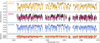 |
Fig. 2 Best-fitting models retrieved for J0835, J0501, and J0500 (top to bottom). The upper three panels show the observational flux in black, and the best-fitting model spectra for the three BDs (J0835, J0501, and J0500). The observed flux is normalised to the mean flux of each order–detector pair after telluric correction. The lower panel shows the residuals between the observed and model spectra. The data and the models are displayed in the rest frame of each object. The shaded region at the top of the image indicates the wavelength coverage of the three detectors for each spectral order (CRIRES+ and K2166 wavelength setting). They slightly differ in the rest-frame of the BDs as presented by the gradient. The sixth order (2321.6-2369.6 nm) is shown because it contains several 12CO and 13CO lines. The data and best-fitting models of the remaining orders can be found in Appendix B. |
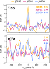 |
Fig. 3 CCFs for 13CO and |
![Mathematical equation: $\[\mathrm{H}_{2}^{18} \mathrm{O}\]$](/articles/aa/full_html/2025/02/aa52859-24/aa52859-24-eq119.png)
5.1 Chemical composition
Our best-fitting spectral models yield the volume mixing ratios (VMRs) of detectable species (see Table 3) in the atmospheres of the three BDs. Constraints are obtained for both H2O and CO for all three targets, leading to a gaseous C and O inventory and subsequent C/O ratio, metallicity, and isotope ratios of the targets. In addition, we present the fluorine abundance for all three BDs.
5.1.1 C/O ratio
The C/O ratio posteriors are shown in Fig. 4, which presents the retrieved values:
![Mathematical equation: $\[\begin{aligned}& \mathrm{C} / \mathrm{O}_{\mathrm{J} 0835}=0.65_{-0.02}^{+0.02} \\& \mathrm{C} / \mathrm{O}_{\mathrm{J} 0501}=0.68_{-0.04}^{+0.04} \\& \mathrm{C} / \mathrm{O}_{\mathrm{J} 0500}=0.71_{-0.01}^{+0.01}.\end{aligned}\]$](/articles/aa/full_html/2025/02/aa52859-24/aa52859-24-eq120.png)
The C/O ratios are comparable among the three BDs, but slightly enhanced compared to the solar C/O ratio (0.59 ± 0.08, Asplund et al. (2021)). This enhancement may be explained by oxygen sequestration, (Line et al. 2021) leading to the condensation of oxygen into silicate-oxide clouds. This scenario was brought up by (de Regt et al. 2024) to explain the increased C/O ratio of ~0.68 of BD DENIS J0255.
In Fig. 4, we compare the retrieved values for the three BDs to the values of other isolated BDs. The C/O ratios retrieved by González Picos et al. (2024) for three young late M-type BDs were within the margins of the solar ratio. In comparison, González Picos et al. (2024) studied M-type objects that have high enough atmospheric temperatures that silicate-oxide clouds do not form, thus explaining their agreement with the solar value. For 2M0355, Zhang et al. (2021b) obtained a C/O ratio using an EC model that accounts for condensation. As such, their C/O ratio, which is in agreement with the solar ratio, represents the bulk elemental abundances.
Using the same EC set-up as de (de Regt et al. 2024), we find bulk C/O ratios of ![Mathematical equation: $\[0.58_{-0.01}^{+0.01}\]$](/articles/aa/full_html/2025/02/aa52859-24/aa52859-24-eq121.png) ,
, ![Mathematical equation: $\[0.60_{-0.05}^{+0.02}\]$](/articles/aa/full_html/2025/02/aa52859-24/aa52859-24-eq122.png) , and
, and ![Mathematical equation: $\[0.60_{-0.01}^{+0.01}\]$](/articles/aa/full_html/2025/02/aa52859-24/aa52859-24-eq123.png) for J0835, J0501, and J0500, respectively. They are in agreement with the solar C/O ratio.
for J0835, J0501, and J0500, respectively. They are in agreement with the solar C/O ratio.
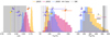 |
Fig. 4 Posterior distributions of the C/O (left), carbon 12C/13C isotope (middle), and oxygen 16O/18O isotope ratio (right) for J0835, J0501, and J0500. The 12C/13C values for the Solar System (terrestrial value) and ISM are 89.3 ± 0.2 (Meija et al. 2016) and 68 ± 16 (Milam et al. 2005), respectively. The C/O value for our Sun is 0.59 ± 0.08 (Asplund et al. 2021). The 16O/18O values for the Solar System and ISM are 557 ± 30 (Wilson 1999) and 525 ± 21 (Lyons et al. 2018). The purple error bars represent the young BDs observed and analysed by González Picos et al. (2024, P1: J1200, P2: TWA28 and P3: J0856), the orange error bar DENIS J0255 (R1) by de Regt et al. (2024), and the yellow 2M0355 (Z1) by Zhang et al. (2022). |
5.1.2 Metallicity
The [C/H] ratio is used as a proxy for metallicity. The derived posterior distributions of [C/H] are shown in the bottom graph of Fig. 5. The [C/H] values are significantly larger than the solar value and other work that used this same proxy (Zhang et al. 2022; González Picos et al. 2024; de Regt et al. 2024). It is unfortunately not straightforward to interpret these values, since metallicities cannot be constrained well with solely K-band high-resolution spectroscopy because of the strong correlation between surface gravity and metallicity in atmospheric retrieval analyses (e.g. González Picos et al. 2024).
5.1.3 Isotope ratios
Constrained 12CO and 13CO abundances were retrieved for all three BDs. From those, the following 12C/13C ratios for J0835, J0501, and J0500 were determined (see Fig. 4):
![Mathematical equation: $\[\begin{aligned}& { }^{12} \mathrm{C} /{ }^{13} \mathrm{C}_{\mathrm{J} 0835}=89_{-11}^{+11} \\& { }^{12} \mathrm{C} /{ }^{13} \mathrm{C}_{\mathrm{J} 0501}=155_{-53}^{+56} \\& { }^{12} \mathrm{C} /{ }^{13} \mathrm{C}_{\mathrm{J} 0500}=117_{-17}^{+20}.\end{aligned}\]$](/articles/aa/full_html/2025/02/aa52859-24/aa52859-24-eq124.png)
The values are similar among the three objects within their 1σ uncertainties. The ratio for J0835 is in agreement with the solar value of 89.3 ± 0.2 (Meija et al. 2016), while the other two objects appear to have slightly larger ratios. All three of them have significantly higher ratios than the present day ISM value 68 ± 16 (Milam et al. 2005). Figure 4 gives an overview of our retrieved ratios in comparison to previous work as part of the SupJup Survey (González Picos et al. 2024; de Regt et al. 2024), and the work on BD 2M0355, the first BD for which the 12C/13C was determined (Zhang et al. 2021b; Zhang et al. 2022).
The ![Mathematical equation: $\[\mathrm{H}_{2}^{18} \mathrm{O}\]$](/articles/aa/full_html/2025/02/aa52859-24/aa52859-24-eq125.png) isotope was included in the retrievals because of the positive detection of
isotope was included in the retrievals because of the positive detection of ![Mathematical equation: $\[\mathrm{H}_{2}^{18} \mathrm{O}\]$](/articles/aa/full_html/2025/02/aa52859-24/aa52859-24-eq126.png) by González Picos et al. (2024) in TWA 28 (16O/18O ~
by González Picos et al. (2024) in TWA 28 (16O/18O ~ ![Mathematical equation: $\[205_{-62}^{+140}\]$](/articles/aa/full_html/2025/02/aa52859-24/aa52859-24-eq127.png) ) and J0856 (16O/18O ~
) and J0856 (16O/18O ~ ![Mathematical equation: $\[141_{-28}^{+42}\]$](/articles/aa/full_html/2025/02/aa52859-24/aa52859-24-eq128.png) ). As mentioned before, only one weak detection was found for J0835. From these retrieved VMRs, we calculated the 16O/18O ratio for J0835:
). As mentioned before, only one weak detection was found for J0835. From these retrieved VMRs, we calculated the 16O/18O ratio for J0835:
![Mathematical equation: $\[{ }^{16} \mathrm{O} /{ }^{18} \mathrm{O}_{\mathrm{J} 0835}=311_{-86}^{+100}.\]$](/articles/aa/full_html/2025/02/aa52859-24/aa52859-24-eq129.png) .
.
Zhang et al. (2021b) and Line et al. (2021) have highlighted the potential of the carbon isotope ratio to serve as an additional diagnostic of planet and BD formation histories. However, evolution on a galactic timescale is also expected to alter the average 12C/13C ratio, since 13C is produced in asymptotic giant branch stars that subsequently enrich the ISM (Iben & Renzini 1983). Therefore, young objects are generally expected to have lower ratios than old objects. Crossfield et al. (2019) find isotopologue ratio measurements for GJ 745 A and B of 12C/13C = 296 ± 45 and 224 ± 26, and 16O/18O = 1220 ± 260 and 1550 ± 360, respectively. Caramazza et al. (2023) suggested, after observing the X-ray emission for GJ 745 A and B, that the extremely low X-ray activity of the binary, their ultra-low metallicity, non-detection of photometric star spot variability, and low chromospheric emission are in line with an older age object. As far as we know, these are the highest carbon and oxygen isotope ratios measured for mature low-mass stars.
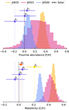 |
Fig. 5 Posterior distributions of the fluorine abundance relative to hydrogen [F/H] (top) and carbon abundance relative to hydrogen [C/H], used as a measure of metallicity (bottom) for J0835, J0501, and J0500. J1200, TWA28, and J0856 are the young BDs observed and analysed by González Picos et al. (2024), DENIS by de Regt et al. (2024), and 2M0355 by Zhang et al. (2022). log10 [F/H]⊙ = −7.6 ± 0.25 (Asplund et al. 2021) and log10 [C/H]⊙ = −3.54 ± 0.04 (Asplund et al. 2021). |
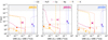 |
Fig. 6 VMRs of line species (12CO, H2O, Ca, Na, Ti, and K) for the three BDs using the FC and EC method. The error bars represent the values retrieved with the FC method. The dashed lines show the Fastchem EC abundances corresponding to the best-fitting P-T profile, C/O ratio, and metallicity for each of the BDs. The EC abundances have a similar line style and colour as those of the associated FC VMR. The black lines indicate the location of the peak of the integrated contribution functions, and the shaded areas indicate the pressures where we expect large uncertainties as we are not sensitive to probe these atmospheric pressures. |
5.1.4 Hydrogen fluoride
The abundances of fluorine with respect to solar were computed from the retrieved VMRs of HF:
![Mathematical equation: $\[\begin{aligned}{[\mathrm{F} / \mathrm{H}]_{\mathrm{J} 0835} } & =0.41_{-0.05}^{+0.05} \\{[\mathrm{F} / \mathrm{H}]_{\mathrm{J} 0501} } & =0.26_{-0.19}^{+0.19} \\{[\mathrm{F} / \mathrm{H}]_{\mathrm{J} 0500} } & =0.07_{-0.06}^{+0.06}.\end{aligned}\]$](/articles/aa/full_html/2025/02/aa52859-24/aa52859-24-eq130.png)
All BDs show a strong HF detection significance: 14.5σ, 4.2σ, and 9.2σ for J0835, J0501, and J0500, respectively.
The computed [F/H] for J0500 is in a 1σ agreement with the solar abundance of ![Mathematical equation: $\[\log _{10}\left(\frac{n_{\mathrm{F}}}{n_{\mathrm{H}}}\right)_{\odot}=-7.6 \pm 0.25\]$](/articles/aa/full_html/2025/02/aa52859-24/aa52859-24-eq131.png) (Asplund et al. 2009), J0501 is in agreement within 2σ, and J0835 shows a higher value for [F/H]. It should be noted that the [F/H] suffers from the same metallicity-surface gravity degeneracy as the [C/H] and thus the absolute fluorine abundance of J0835 is not necessarily super-solar.
(Asplund et al. 2009), J0501 is in agreement within 2σ, and J0835 shows a higher value for [F/H]. It should be noted that the [F/H] suffers from the same metallicity-surface gravity degeneracy as the [C/H] and thus the absolute fluorine abundance of J0835 is not necessarily super-solar.
For our K-band observations, we are sensitive to the HF 10 vibrational transitions, as it has prominent absorption lines in the 2.3–2.5 μm region (Wilzewski et al. 2016). Recent work in the SupJup Survey, operating in the K band, has revealed the presence of HF in several sub-stellar objects (González Picos et al. 2024; de Regt et al., in prep.; Zhang et al. 2024). Figure 5 gives an overview of all values obtained so far.
5.2 Free chemistry versus equilibrium chemistry
As elaborated in Sect. 4.4, the FC method (e.g. de Regt et al. 2024; González Picos et al. 2024) was applied. This method assumes a constant-with-altitude mixing ratio for every species in the model atmospheres. Despite the FC method providing a good approximation for our spectra, it is insightful to compare our retrieved abundances against those predicted by EC. The EC method assumed element abundances as retrieved from the pRT models (see Fig. 6).
Using FastChem (Stock et al. 2018, 2022; Kitzmann et al. 2024) we compared our retrieved mixing ratios against EC predictions. The VMRs (see Fig. 6) are normalised relative to the VMR of 12CO, which corrects for any potential systematic offsets due to the metallicity-surface gravity degeneracy (González Picos et al. 2024; de Regt et al. 2024). The H2O abundance retrieved with the FC method deviates slightly from the EC predictions, which could indicate the presence of quenching and/or disequilibrium chemistry.
Besides the line species presented in Table 3 various pRT models including the atomic species Na, Ti and K were tested against the spectra. The Na and K, or alkali lines, have been found to be a very good probe for differences in surface gravity for late-type objects (Gorlova et al. 2003; Schlieder et al. 2012; Allers & Liu 2013; Martin et al. 2017; Manjavacas et al. 2020). For young BDs, alkali lines have been observed to be weaker than for field BDs (Steele & Jameson 1995; Gorlova et al. 2003; Allers et al. 2007; Allers & Liu 2013; Bonnefoy et al. 2014).
The atomic opacities from Na, K (Allard et al. 2019), and Ti (Castelli & Kurucz 2003) were included in our FC retrievals, but not detected. The retrieved abundances using the FC models are displayed by the error bars in Fig. 6. The dashed lines represent those for the EC models. Indeed, the derived VMR upper limits for Na, Ti, and K are in line with those expected from the EC models.
The H2O, Na and K EC abundances of J0835 and J0500 are skewed for smaller pressures. For lower temperatures, CH4 becomes the dominating carbon species, yielding a drop-off for the CO abundances. The increase in the relative H2O abundances is expected since the models are normalised towards CO. We retrieved a lower temperature in the upper atmosphere of J0835 than J0500, which explains the drop-off location for J0835 to be at a higher pressure. For J0501, the temperature does not get low enough to see this CO-CH4 switch. Even though we retrieve these abundances, the presence of a similar shift is unlikely due to the vertical mixing in the atmospheres (Zahnle & Marley 2014).
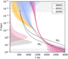 |
Fig. 7 Best-fit P–T profiles (solid lines) for BDs J0835, J0501, and J0500. The associated shaded regions indicate the 1σ, 2σ, and 3σ regions. The integrated contribution functions are indicated on the left vertical axis. Two self-consistent Sonora elf owl P-T profiles, SE1 (Teff = 1800 K, log g = 5.5) and SE2 (Teff = 1700 K, log g = 4.5) are overplotted with dashed black lines. |
5.3 Thermal profile
The best-fitting P-T profiles (the solid line and the shaded areas indicate the 1σ, 2σ, and 3σ uncertainties in Fig. 7) of the BDs J0835 and J0500 are similar, while the profile of J0501 is warmer by ~100 K at similar pressures. Since the retrieved surface gravity of J0501 is lower than that of the others by an order of magnitude, the photospheric region, as indicated by the integrated contribution function (shaded area on the left in Fig. 7), is found to be located at lower pressures (order of ~10). This is in line with the mass and radii estimates for the three targets by Filippazzo et al. (2015), where J0501 is found to be of significantly lower mass and larger radius. As expected, the confidence envelopes of the P-T profile show larger uncertainties outside the photosphere, at the higher and lower altitudes. These regions are not probed by the K-band spectrum.
The self-consistent Sonora elf owl models (SE1 and SE2 in Fig. 7) were calculated using Teff = 1800 K and log g = 5.5, and Teff = 1700 K and log g = 4.5, both assuming a solar metallicity and C/O ratio. Just as found for YSES 1b (Zhang et al. 2024), the retrieved P-T profiles are more isothermal than the self-consistent models. This may indicate the absence of continuum opacity, for example clouds, since a spectrum of a cloudless atmosphere combined with an isothermal temperature gradient is equivalent to a spectrum of a cloudy atmosphere.
To a first order, the retrieved thermal profiles for all three objects seem to agree well with the literature values for the effective temperature of each object (see Table 1). A direct comparison of our profiles to the literature values is unfavorable, due to the disparate methods used to derive the literature values.
5.4 Surface gravity
The retrieved values for the surface gravity, log g, are in line with the expectations for young, low-surface gravity objects (Baraffe et al. 2002; Allers et al. 2007; Bonnefoy et al. 2014). While the surface gravity values for J0835 and J0500 are similar, J0501 shows a significantly lower value. This explains the shift of the emission contribution towards lower pressures. Unfortunately, the limited spectral range of the K band makes these types of observations less sensitive to log g. The surface gravity, metallicity, and effective temperature govern the atmospheric gaseous optical depth of an object. Since the atmospheric scale height is inversely proportional to the surface gravity, the latter influences the pressure range of the photosphere. Therefore, it plays a significant role in shaping the observed spectra as it affects line shapes, temperature profiles, and the overall continuum (Marley & Robinson 2015; Mukherjee et al. 2024). González Picos et al. (2024) show that the posterior distributions of surface gravities and metallicities exhibit a high degree of degeneracy in the K band, as we also notice for our targets, hampering an accurate constraint.
5.5 Rotational velocity
J0835 has a rotational velocity of
![Mathematical equation: $\[v ~\sin~ i_\text{J0835}=15.42_{-0.12}^{+0.14} \mathrm{~km} \mathrm{~s}^{-1}.\]$](/articles/aa/full_html/2025/02/aa52859-24/aa52859-24-eq132.png)
It is the fastest rotator of our small sample, as is also apparent from the broadened spectral features in Fig. 2. Blake et al. (2010) reported a similar value for the projected rotational velocity of v sin iJ0835 = 14.18 ± 0.43 km s−1. For J0500 we retrieve a value of
![Mathematical equation: $\[v ~\sin~ i_{\mathrm{J} 0500}=5.05_{-0.16}^{+0.21} \mathrm{~km} \mathrm{~s}^{-1},\]$](/articles/aa/full_html/2025/02/aa52859-24/aa52859-24-eq133.png)
while Blake et al. (2010) finds v sin iJ0500 = 9.65 ± 0.36 km s−1. A possible explanation for this difference could be that the lower spectral resolution of Blake et al. (2010, R~35 000) hinders the measurement of low projected rotational velocities.
J0501 has a retrieved projected rotational velocity of
![Mathematical equation: $\[v ~\sin~ i_{\mathrm{J} 0501}=6.90_{-0.24}^{+0.25} \mathrm{~km} \mathrm{~s}^{-1},\]$](/articles/aa/full_html/2025/02/aa52859-24/aa52859-24-eq134.png)
which is also lower than the velocity found by Vos et al. (2020), ![Mathematical equation: $\[9.57_{-0.58}^{+0.67}\]$](/articles/aa/full_html/2025/02/aa52859-24/aa52859-24-eq135.png) km s−1, which was based on Gemini Near-InfraRed Spectrograph (GNIRS; Elias et al. 2006b,a) high-resolution observations with R~18 000. Again, the higher resolution of our CRIRES+ observations likely aids in resolving such a low rotational velocity.
km s−1, which was based on Gemini Near-InfraRed Spectrograph (GNIRS; Elias et al. 2006b,a) high-resolution observations with R~18 000. Again, the higher resolution of our CRIRES+ observations likely aids in resolving such a low rotational velocity.
The projected rotational velocities are consistent with the expected slow rotation of young, bloated BDs. However, their intrinsic rotation velocities also depend on viewing angle. Similar to González Picos et al. (2024), there is a tentative relation between our GP parameters and the v sin i. Slower rotators exhibit smaller GP length-scales, ℓ, and larger amplitudes, a, compared to fast rotators. This is as expected from the fact that for fast rotators, differences between model and observations will be smeared out over more spectral pixels, resulting in lower GP amplitudes and larger length-scales.
6 Conclusions and future work
We analysed high-resolution CRIRES+ spectra for three young BDs, providing insights into their atmospheric composition. Their C/O ratios are somewhat higher than that of the Sun, which could be the result of oxygen sequestration. Their metallicities are also higher by a factor of a few compared to the Sun. However, uncertainties may be underestimated due to the known correlation with surface gravity, to which these K-band observations are not very sensitive.
Performing precise measurements of isotope ratios is a challenge. However, we were able to constrain the isotopic composition of the BDs. The 12C/13C ratios for J0835, J0501, and J0500 are ![Mathematical equation: $\[93_{-10}^{+10}\]$](/articles/aa/full_html/2025/02/aa52859-24/aa52859-24-eq136.png) (9.1σ),
(9.1σ), ![Mathematical equation: $\[155_{-53}^{+56}\]$](/articles/aa/full_html/2025/02/aa52859-24/aa52859-24-eq137.png) (3.0σ), and
(3.0σ), and ![Mathematical equation: $\[117_{-17}^{+20}\]$](/articles/aa/full_html/2025/02/aa52859-24/aa52859-24-eq138.png) (6.8σ), respectively. All values suggest a slightly depleted 13CO concentration compared to that of the local ISM.
(6.8σ), respectively. All values suggest a slightly depleted 13CO concentration compared to that of the local ISM.
The remaining observational data of the SupJup Survey are being analysed, including tens of other BDs and SJs, to constrain their C/O, 12C/13C, and 16O/18O ratios.
Data availability
Appendix A and Appendix B, including graphs and tables, are published in the Zenodo repository: http://doi.org/10.5281/zenodo.14713641.
Acknowledgements
W.M. acknowledges funding from NWO grant from the second round of the Planetary and Exoplanetary Science Programme (PEPSciII). S.d.R. and I.S. acknowledge funding from NWO grant OCENW.M.21.010. We thank the SURF Cooperative (www.surf.nl) for the support in using the National Supercomputer Snellius using grant no. EINF-4556 and EINF-9460. This research has made use of the following software: Astropy (Astropy Collaboration 2022), corner (Foreman-Mackey 2016), Matplotlib (Hunter 2007), MultiNest (Feroz et al. 2019), NumPy (Harris et al. 2020), petitRADTRANS (Mollière et al. 2019), picaso (Mukherjee et al. 2023), PyAstronomy (Czesla et al. 2019), and PyMultiNest (Buchner et al. 2014).
Appendix A Posterior distributions of atmospheric retrieval BDs
Supplementary graphs and tables are stored in the Zenodo repository: https://zenodo.org/records/14713641
Appendix B Best-fitting spectra
Supplementary graphs are stored in the Zenodo repository: https://zenodo.org/records/14713641
Appendix C Cross-correlation analysis of 12CO, 13CO, ![Mathematical equation: $\[\mathrm{H}_{2}^{16} \mathrm{O}\]$](/articles/aa/full_html/2025/02/aa52859-24/aa52859-24-eq139.png) ,
, ![Mathematical equation: $\[\mathrm{H}_{2}^{18} \mathrm{O}\]$](/articles/aa/full_html/2025/02/aa52859-24/aa52859-24-eq140.png) , HF, and Ca abundances
, HF, and Ca abundances
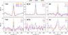 |
Fig. C.1 CCFs for 12CO, 13CO, |
![Mathematical equation: $\[\mathrm{H}_{2}^{16} \mathrm{O}\]$](/articles/aa/full_html/2025/02/aa52859-24/aa52859-24-eq141.png)
![Mathematical equation: $\[\mathrm{H}_{2}^{18} \mathrm{O}\]$](/articles/aa/full_html/2025/02/aa52859-24/aa52859-24-eq142.png)
References
- Allard, N. F., Spiegelman, F., Leininger, T., & Molliere, P. 2019, A&A, 628, A120 [NASA ADS] [CrossRef] [EDP Sciences] [Google Scholar]
- Allers, K. N., & Liu, M. C. 2013, ApJ, 772, 79 [NASA ADS] [CrossRef] [Google Scholar]
- Allers, K. N., Jaffe, D. T., Luhman, K. L., et al. 2007, ApJ, 657, 511 [Google Scholar]
- Andrei, A. H., Smart, R. L., Penna, J. L., et al. 2011, AJ, 141, 54 [Google Scholar]
- Asplund, M., Grevesse, N., Sauval, A. J., & Scott, P. 2009, A&A Rev., 47, 481 [Google Scholar]
- Asplund, M., Amarsi, A. M., & Grevesse, N. 2021, A&A, 653, A141 [NASA ADS] [CrossRef] [EDP Sciences] [Google Scholar]
- Astropy Collaboration (Price-Whelan, A. M., et al.) 2022, ApJ, 935, 167 [NASA ADS] [CrossRef] [Google Scholar]
- Baraffe, I., Chabrier, G., Allard, F., & Hauschildt, P. H. 2002, A&A, 382, 563 [CrossRef] [EDP Sciences] [Google Scholar]
- Barman, T. S., Macintosh, B., Konopacky, Q. M., & Marois, C. 2011, ApJ, 733, 65 [Google Scholar]
- Bate, M. R., Bonnell, I. A., & Bromm, V. 2002, MNRAS, 332, L65 [NASA ADS] [CrossRef] [Google Scholar]
- Benneke, B., & Seager, S. 2013, ApJ, 778, 153 [Google Scholar]
- Bergin, E. A., Bosman, A., Teague, R., et al. 2024, ApJ, 965, 147 [NASA ADS] [CrossRef] [Google Scholar]
- Best, W. M. J., Dupuy, T. J., Liu, M. C., et al. 2024, https://doi.org/10.5281/zenodo.13993077 [Google Scholar]
- Blake, C. H., Charbonneau, D., & White, R. J. 2010, ApJ, 723, 684 [Google Scholar]
- Bonnefoy, M., Chauvin, G., Lagrange, A. M., et al. 2014, A&A, 562, A127 [NASA ADS] [CrossRef] [EDP Sciences] [Google Scholar]
- Borysow, J., Frommhold, L., & Birnbaum, G. 1988, ApJ, 326, 509 [NASA ADS] [CrossRef] [Google Scholar]
- Brogi, M., & Line, M. R. 2019, AJ, 157, 114 [Google Scholar]
- Brogi, M., Snellen, I. A. G., de Kok, R. J., et al. 2012, Nature, 486, 502 [Google Scholar]
- Brogi, M., de Kok, R. J., Albrecht, S., et al. 2016, ApJ, 817, 106 [Google Scholar]
- Buchner, J., Georgakakis, A., Nandra, K., et al. 2014, A&A, 564, A125 [NASA ADS] [CrossRef] [EDP Sciences] [Google Scholar]
- Burgasser, A. J., Cruz, K. L., Cushing, M., et al. 2010, ApJ, 710, 1142 [Google Scholar]
- Burningham, B., Marley, M. S., Line, M. R., et al. 2017, MNRAS, 470, 1177 [NASA ADS] [CrossRef] [Google Scholar]
- Caramazza, M., Stelzer, B., Magaudda, E., et al. 2023, A&A, 676, A14 [NASA ADS] [CrossRef] [EDP Sciences] [Google Scholar]
- Castelli, F., & Kurucz, R. L. 2003, in Modelling of Stellar Atmospheres (Cambridge: Cambrigde University Press), 210 [Google Scholar]
- Chan, Y. M., & Dalgarno, A. 1965, Proc. Phys. Soc., 85, 227 [NASA ADS] [CrossRef] [Google Scholar]
- Clayton, D. D., & Nittler, L. R. 2004, A&A Rev., 42, 39 [Google Scholar]
- Coxon, J. A., & Hajigeorgiou, P. G. 2024, J. Phys. B: At. Mol. Opt. Phys., 57, 133 [Google Scholar]
- Cridland, A. J., Pudritz, R. E., & Alessi, M. 2016, MNRAS, 461, 3274 [Google Scholar]
- Crossfield, I. J. M., Lothringer, J. D., Flores, B., et al. 2019, ApJ, 871, L3 [NASA ADS] [CrossRef] [Google Scholar]
- Cruz, K. L., Reid, I. N., Liebert, J., Kirkpatrick, J. D., & Lowrance, P. J. 2003, AJ, 126, 2421 [Google Scholar]
- Cruz, K. L., Kirkpatrick, J. D., & Burgasser, A. J. 2009, AJ, 137, 3345 [NASA ADS] [CrossRef] [Google Scholar]
- Currie, T., Burrows, A., Itoh, Y., et al. 2011, ApJ, 729, 128 [Google Scholar]
- Cutri, R. M., Skrutskie, M. F., van Dyk, S., et al. 2003, VizieR Online Data Catalog: II/246 [Google Scholar]
- Czesla, S., Schröter, S., Schneider, C. P., et al. 2019, Astrophysics Source Code Library [record ascl:1906.010] [Google Scholar]
- Dalgarno, A., & Williams, D. A. 1962, ApJ, 136, 690 [NASA ADS] [CrossRef] [Google Scholar]
- Delorme, J.-R., Jovanovic, N., Echeverri, D., et al. 2021, J. Astron. Telesc. Instrum. Syst., 7, 035006 [NASA ADS] [CrossRef] [Google Scholar]
- de Regt, S., Gandhi, S., Snellen, I. A. G. F., et al. 2024, A&A, 688, A116 [NASA ADS] [CrossRef] [EDP Sciences] [Google Scholar]
- Dorn, R. J., Anglada-Escude, G., Baade, D., et al. 2014, The Messenger, 156, 7 [NASA ADS] [Google Scholar]
- Dorn, R. J., Bristow, P., Smoker, J. V., et al. 2023, A&A, 671, A24 [NASA ADS] [CrossRef] [EDP Sciences] [Google Scholar]
- Elias, J. H., Joyce, R. R., Liang, M., et al. 2006a, Proc. SPIE, 6269, 62694C [CrossRef] [Google Scholar]
- Elias, J. H., Rodgers, B., Joyce, R. R., et al. 2006b, Proc. SPIE, 6269, 626914 [CrossRef] [Google Scholar]
- Faherty, J. K., Riedel, A. R., Cruz, K. L., et al. 2016, ApJS, 225, 10 [Google Scholar]
- Feroz, F., Hobson, M. P., Cameron, E., & Pettitt, A. N. 2019, OJAp, 2, 10 [Google Scholar]
- Filippazzo, J. C., Rice, E. L., Faherty, J., et al. 2015, ApJ, 810, 158 [Google Scholar]
- Foreman-Mackey, D. 2016, J. Open Source Softw., 1, 24 [Google Scholar]
- Freytag, B., Allard, F., Ludwig, H.-G., Homeier, D., & Steffen, M. 2010, A&A, 513, A19 [NASA ADS] [CrossRef] [EDP Sciences] [Google Scholar]
- Gagné, J., Faherty, J. K., Cruz, K. L., et al. 2015, ApJS, 219, 33 [CrossRef] [Google Scholar]
- Gaia Collaboration 2020, VizieR On-line Data Catalog: I/350 [Google Scholar]
- Gandhi, S., de Regt, S., Snellen, I. A. G., et al. 2023, ApJ, 957, L36 [NASA ADS] [CrossRef] [Google Scholar]
- González Picos, D., Snellen, I. A. G., de Regt, S., et al. 2024, A&A, 689, A212 [NASA ADS] [CrossRef] [EDP Sciences] [Google Scholar]
- Gorlova, N. I., Meyer, M. R., Rieke, G. H., & Liebert, J. 2003, ApJ, 593, 1074 [NASA ADS] [CrossRef] [Google Scholar]
- Gray, D. F. 2008, The Observation and Analysis of Stellar Photospheres (Cambridge: Cambridge University Press) [Google Scholar]
- Harris, C. R., Millman, K. J., van der Walt, S. J., et al. 2020, Nature, 585, 357 [NASA ADS] [CrossRef] [Google Scholar]
- Helled, R., Bodenheimer, P., Podolak, M., et al. 2014, Giant Planet Formation, Evolution, and Internal Structure (Tucson: University of Arizona Press) [Google Scholar]
- Hoeijmakers, H. J., Seidel, J. V., Pino, L., et al. 2020, A&A, 641, A123 [NASA ADS] [CrossRef] [EDP Sciences] [Google Scholar]
- Horne, K. 1986, PASP, 98, 609 [Google Scholar]
- Hunter, J. D. 2007, CiSE, 9, 90 [Google Scholar]
- Iben, I., J., & Renzini, A. 1983, ARA&A, 21, 271 [NASA ADS] [CrossRef] [Google Scholar]
- Janson, M., Bergfors, C., Goto, M., Brandner, W., & Lafrenière, D. 2010, ApJ, 710, L35 [NASA ADS] [CrossRef] [Google Scholar]
- Kaeufl, H.-U., Ballester, P., Biereichel, P., et al. 2004, Proc. SPIE, Vol. 5492, 1218 [NASA ADS] [CrossRef] [Google Scholar]
- Kawahara, H., Kawashima, Y., Masuda, K., et al. 2022, ApJS, 258, 31 [NASA ADS] [CrossRef] [Google Scholar]
- Kirkpatrick, J. D., Cruz, K. L., Barman, T. S., et al. 2008, ApJ, 689, 1295 [NASA ADS] [CrossRef] [Google Scholar]
- Kitzmann, D., Stock, J. W., & Patzer, A. B. C. 2024, MNRAS, 527, 7263 [Google Scholar]
- Koen, C., Matsunaga, N., & Menzies, J. 2004, MNRAS, 354, 466 [NASA ADS] [CrossRef] [Google Scholar]
- Landman, R., Stolker, T., Snellen, I. A. G., et al. 2024, A&A, 682, A48 [NASA ADS] [CrossRef] [EDP Sciences] [Google Scholar]
- Langer, W. D., & Penzias, A. A. 1993, ApJ, 408, 539 [NASA ADS] [CrossRef] [Google Scholar]
- Li, G., Gordon, I. E., Le Roy, R. J., et al. 2013, J. Quant. Spectrosc. Radiat. Transfer, 121, 78 [NASA ADS] [CrossRef] [Google Scholar]
- Li, G., Gordon, I. E., Rothman, L. S., et al. 2015, ApJS, 216, 15 [NASA ADS] [CrossRef] [Google Scholar]
- Line, M. R., Brogi, M., Bean, J. L., et al. 2021, Nature, 598, 580 [NASA ADS] [CrossRef] [Google Scholar]
- Liu, M. C., Dupuy, T. J., & Allers, K. N. 2016, ApJ, 833, 96 [NASA ADS] [CrossRef] [Google Scholar]
- Lothringer, J. D., Rustamkulov, Z., Sing, D. K., et al. 2021, ApJ, 914, 12 [CrossRef] [Google Scholar]
- Ludwig, H. G., Allard, F., & Hauschildt, P. H. 2006, A&A, 459, 599 [NASA ADS] [CrossRef] [EDP Sciences] [Google Scholar]
- Lyons, J., Gharib-Nezhad, E., & Ayres, T. 2018, Nat. Commun., 9, 908 [CrossRef] [Google Scholar]
- Madhusudhan, N. 2012, ApJ, 758, 36 [NASA ADS] [CrossRef] [Google Scholar]
- Madhusudhan, N., Harrington, J., Stevenson, K. B., et al. 2010, Nature, 469, 64 [Google Scholar]
- Manjavacas, E., Lodieu, N., Béjar, V. J. S., et al. 2020, MNRAS, 491, 5925 [NASA ADS] [CrossRef] [Google Scholar]
- Marley, M. S., & Robinson, T. D. 2015, ARA&A, 53, 279 [Google Scholar]
- Martin, E. C., Mace, G. N., McLean, I. S., et al. 2017, ApJ, 838, 73 [NASA ADS] [CrossRef] [Google Scholar]
- Meija, J., Coplen, T. B., Berglund, M., et al. 2016, PAC, 88, 265 [Google Scholar]
- Milam, S. N., Savage, C., Brewster, M. A., Ziurys, L. M., & Wyckoff, S. 2005, ApJ, 634, 1126 [Google Scholar]
- Miles, B. E., Biller, B. A., Patapis, P., et al. 2023, ApJ, 946, L6 [NASA ADS] [CrossRef] [Google Scholar]
- Mollière, P., Wardenier, J. P., van Boekel, R., et al. 2019, A&A, 627, A67 [Google Scholar]
- Mollière, P., Stolker, T., Lacour, S., et al. 2020, A&A, 640, A131 [Google Scholar]
- Mollière, P., Molyarova, T., Bitsch, B., et al. 2022, ApJ, 934, 74 [CrossRef] [Google Scholar]
- Mukherjee, S., Batalha, N. E., Fortney, J. J., & Marley, M. S. 2023, ApJ, 942, 71 [NASA ADS] [CrossRef] [Google Scholar]
- Mukherjee, S., Fortney, J., Morley, C., et al. 2024, ApJ, 963, 73 [NASA ADS] [CrossRef] [Google Scholar]
- Oberg, K. I., Murray-Clay, R., & Bergin, E. A. 2011, ApJ, 743, L16 [NASA ADS] [CrossRef] [Google Scholar]
- Oppenheimer, B. R., Baranec, C., Beichman, C., et al. 2013, ApJ, 768, 24 [NASA ADS] [CrossRef] [Google Scholar]
- Paufique, J., Biereichel, P., Donaldson, R., et al. 2004, Proc. SPIE, 5490, 216 [CrossRef] [Google Scholar]
- Piso, A.-M. A., Öberg, K. I., Birnstiel, T., & Murray-Clay, R. A. 2015, ApJ, 815, 109 [Google Scholar]
- Pollack, J. B., Hubickyj, O., Bodenheimer, P., et al. 1996, Icarus, 124, 62 [NASA ADS] [CrossRef] [Google Scholar]
- Polyansky, O. L., Kyuberis, A. A., Lodi, L., et al. 2017, VizieR Online Data Catalog: J/MNRAS/466/1363 [NASA ADS] [Google Scholar]
- Polyansky, O. L., Kyuberis, A. A., Zobov, N. F., et al. 2018, MNRAS, 480, 2597 [NASA ADS] [CrossRef] [Google Scholar]
- Reid, I. N., Cruz, K. L., Kirkpatrick, J. D., et al. 2008, AJ, 136, 1290 [Google Scholar]
- Rothman, L. S., Gordon, I. E., Barber, R. J., et al. 2010, J. Quant. Spectrosc. Radiat. Transfer, 111, 2139 [NASA ADS] [CrossRef] [Google Scholar]
- Ruffio, J.-B., Macintosh, B., Konopacky, Q. M., et al. 2019, AJ, 158, 200 [Google Scholar]
- Sanghi, A., Liu, M. C., Best, W. M. J., et al. 2023, ApJ, 959, 63 [NASA ADS] [CrossRef] [Google Scholar]
- Schlawin, E., Burgasser, A. J., Karalidi, T., Gizis, J. E., & Teske, J. 2017, ApJ, 849, 163 [NASA ADS] [CrossRef] [Google Scholar]
- Schlieder, J. E., Lépine, S., Rice, E., et al. 2012, AJ, 143, 114 [NASA ADS] [CrossRef] [Google Scholar]
- Schwarz, H., Ginski, C., de Kok, Remco J., et al. 2016, A&A, 593, A74 [NASA ADS] [CrossRef] [EDP Sciences] [Google Scholar]
- Skemer, A. J., Hinz, P. M., Esposito, S., et al. 2012, ApJ, 753, 14 [Google Scholar]
- Smette, A., Sana, H., Noll, S., et al. 2015, A&A, 576, A77 [NASA ADS] [CrossRef] [EDP Sciences] [Google Scholar]
- Snellen, I. A. G., Brandl, B. R., de Kok, R. J., et al. 2014, Nature, 509, 63 [Google Scholar]
- Somogyi, W., Yurchenko, S. N., & Yachmenev, A. 2021, J. Chem. Phys., 155, 214303 [NASA ADS] [CrossRef] [Google Scholar]
- Steele, I. A., & Jameson, R. F. 1995, MNRAS, 272, 630 [NASA ADS] [Google Scholar]
- Stock, J. W., Kitzmann, D., Patzer, A. B. C., & Sedlmayr, E. 2018, MNRAS, 479, 865 [NASA ADS] [Google Scholar]
- Stock, J. W., Kitzmann, D., & Patzer, A. B. C. 2022, MNRAS, 517, 4070 [NASA ADS] [CrossRef] [Google Scholar]
- Tsuji, T., Ohnaka, K., Aoki, W., & Nakajima, T. 1996, A&A, 308, L29 [NASA ADS] [Google Scholar]
- Turrini, D., Schisano, E., Fonte, S., et al. 2021, ApJ, 909, 40 [Google Scholar]
- Visscher, C., Lodders, K., & Fegley, Bruce, J. 2010, ApJ, 716, 1060 [NASA ADS] [CrossRef] [Google Scholar]
- Vos, J. M., Biller, B. A., Allers, K. N., et al. 2020, AJ, 160, 38 [NASA ADS] [CrossRef] [Google Scholar]
- Wang, J. J., Ruffio, J.-B., Morris, E., et al. 2021, AJ, 162, 148 [NASA ADS] [CrossRef] [Google Scholar]
- Whitworth, A., Bate, M. R., Nordlund, Å., Reipurth, B., & Zinnecker, H. 2007, in Protostars and Planets V, eds. B. Reipurth, D. Jewitt, & K. Keil (Tucson: University of Arizona Press), 459 [Google Scholar]
- Wilson, T. L. 1999, Rep. Prog. Phys., 62, 143 [Google Scholar]
- Wilson, P. A., Rajan, A., & Patience, J. 2014, A&A, 566, A111 [NASA ADS] [CrossRef] [EDP Sciences] [Google Scholar]
- Wilzewski, J. S., Gordon, I. E., Kochanov, R. V., Hill, C., & Rothman, L. S. 2016, J. Quant. Spectrosc. Radiat. Transfer, 168, 193 [NASA ADS] [CrossRef] [Google Scholar]
- Woods, P. M., & Willacy, K. 2009, ApJ, 693, 1360 [Google Scholar]
- Xuan, J. W., Wang, J., Ruffio, J.-B., et al. 2022, ApJ, 937, 54 [NASA ADS] [CrossRef] [Google Scholar]
- Zahnle, K. J., & Marley, M. S. 2014, ApJ, 797, 41 [CrossRef] [Google Scholar]
- Zapatero Osorio, M. R., Béjar, V. J. S., Miles-Páez, P. A., et al. 2014, A&A, 568, A6 [NASA ADS] [CrossRef] [EDP Sciences] [Google Scholar]
- Zhang, Y., Snellen, I. A. G., Bohn, A. J., et al. 2021a, Nature, 595, 370 [NASA ADS] [CrossRef] [Google Scholar]
- Zhang, Y., Snellen, I. A. G., & Mollière, P. 2021b, A&A, 656, A76 [NASA ADS] [CrossRef] [EDP Sciences] [Google Scholar]
- Zhang, Y., Snellen, I. A. G., Brogi, M., & Birkby, J. L. 2022, RNAAS, 6, 194 [NASA ADS] [Google Scholar]
- Zhang, Z., Mollière, P., Hawkins, K., et al. 2023, AJ, 166, 198 [NASA ADS] [CrossRef] [Google Scholar]
- Zhang, Y., González Picos, D., de Regt, S., et al. 2024, AJ, 168, 246 [NASA ADS] [CrossRef] [Google Scholar]
All Tables
All Figures
|
Fig. 1 Colour-magnitude diagram of MJ vs J − K showing the observed low- and planetary-mass objects of the ESO SupJup Survey. The companions and their hosts are pictured as black hexagons and diamonds, respectively. All 19 observed isolated BDs are marked as black-outlined circles, and the colour denotes their spectral type. The same colour coding is used for the population of isolated cool dwarfs indicated in the background. These objects, originating from the UltracoolSheet (Best et al. 2024), are shown as a reference. |
| In the text | |
|
Fig. 2 Best-fitting models retrieved for J0835, J0501, and J0500 (top to bottom). The upper three panels show the observational flux in black, and the best-fitting model spectra for the three BDs (J0835, J0501, and J0500). The observed flux is normalised to the mean flux of each order–detector pair after telluric correction. The lower panel shows the residuals between the observed and model spectra. The data and the models are displayed in the rest frame of each object. The shaded region at the top of the image indicates the wavelength coverage of the three detectors for each spectral order (CRIRES+ and K2166 wavelength setting). They slightly differ in the rest-frame of the BDs as presented by the gradient. The sixth order (2321.6-2369.6 nm) is shown because it contains several 12CO and 13CO lines. The data and best-fitting models of the remaining orders can be found in Appendix B. |
| In the text | |
|
Fig. 3 CCFs for 13CO and |
| In the text | |
|
Fig. 4 Posterior distributions of the C/O (left), carbon 12C/13C isotope (middle), and oxygen 16O/18O isotope ratio (right) for J0835, J0501, and J0500. The 12C/13C values for the Solar System (terrestrial value) and ISM are 89.3 ± 0.2 (Meija et al. 2016) and 68 ± 16 (Milam et al. 2005), respectively. The C/O value for our Sun is 0.59 ± 0.08 (Asplund et al. 2021). The 16O/18O values for the Solar System and ISM are 557 ± 30 (Wilson 1999) and 525 ± 21 (Lyons et al. 2018). The purple error bars represent the young BDs observed and analysed by González Picos et al. (2024, P1: J1200, P2: TWA28 and P3: J0856), the orange error bar DENIS J0255 (R1) by de Regt et al. (2024), and the yellow 2M0355 (Z1) by Zhang et al. (2022). |
| In the text | |
|
Fig. 5 Posterior distributions of the fluorine abundance relative to hydrogen [F/H] (top) and carbon abundance relative to hydrogen [C/H], used as a measure of metallicity (bottom) for J0835, J0501, and J0500. J1200, TWA28, and J0856 are the young BDs observed and analysed by González Picos et al. (2024), DENIS by de Regt et al. (2024), and 2M0355 by Zhang et al. (2022). log10 [F/H]⊙ = −7.6 ± 0.25 (Asplund et al. 2021) and log10 [C/H]⊙ = −3.54 ± 0.04 (Asplund et al. 2021). |
| In the text | |
|
Fig. 6 VMRs of line species (12CO, H2O, Ca, Na, Ti, and K) for the three BDs using the FC and EC method. The error bars represent the values retrieved with the FC method. The dashed lines show the Fastchem EC abundances corresponding to the best-fitting P-T profile, C/O ratio, and metallicity for each of the BDs. The EC abundances have a similar line style and colour as those of the associated FC VMR. The black lines indicate the location of the peak of the integrated contribution functions, and the shaded areas indicate the pressures where we expect large uncertainties as we are not sensitive to probe these atmospheric pressures. |
| In the text | |
|
Fig. 7 Best-fit P–T profiles (solid lines) for BDs J0835, J0501, and J0500. The associated shaded regions indicate the 1σ, 2σ, and 3σ regions. The integrated contribution functions are indicated on the left vertical axis. Two self-consistent Sonora elf owl P-T profiles, SE1 (Teff = 1800 K, log g = 5.5) and SE2 (Teff = 1700 K, log g = 4.5) are overplotted with dashed black lines. |
| In the text | |
|
Fig. C.1 CCFs for 12CO, 13CO, |
| In the text | |
Current usage metrics show cumulative count of Article Views (full-text article views including HTML views, PDF and ePub downloads, according to the available data) and Abstracts Views on Vision4Press platform.
Data correspond to usage on the plateform after 2015. The current usage metrics is available 48-96 hours after online publication and is updated daily on week days.
Initial download of the metrics may take a while.