| Issue |
A&A
Volume 696, April 2025
|
|
|---|---|---|
| Article Number | A225 | |
| Number of page(s) | 16 | |
| Section | Planets, planetary systems, and small bodies | |
| DOI | https://doi.org/10.1051/0004-6361/202453190 | |
| Published online | 25 April 2025 | |
The ESO SupJup Survey
VII. Clouds and line asymmetries in CRIRES+ J-band spectra of the Luhman 16 binary
1
Leiden Observatory, Leiden University,
PO Box 9513,
2300
RA
Leiden,
The Netherlands
2
LIRA, Observatoire de Paris, Université PSL, Sorbonne Université, Sorbonne Paris Cité, CNRS,
61 Avenue de l’Observatoire,
75014
Paris,
France
3
Institut d’Astrophysique de Paris, UMR7095, CNRS, Université Paris VI,
98bis Boulevard Arago,
75014
Paris,
France
4
Department of Physics, University of Warwick,
Coventry
CV4 7AL,
UK
5
Centre for Exoplanets and Habitability, University of Warwick,
Gibbet Hill Road,
Coventry
CV4 7AL,
UK
6
Max-Planck-Institut für Astronomie,
Königstuhl 17,
69117
Heidelberg,
Germany
7
School of Physics, Trinity College Dublin, University of Dublin,
Dublin 2,
Ireland
8
Department of Astronomy, California Institute of Technology,
Pasadena,
CA
91125,
USA
★ Corresponding author; This email address is being protected from spambots. You need JavaScript enabled to view it.
Received:
27
November
2024
Accepted:
22
March
2025
Abstract
Context. Brown dwarfs at the L–T transition likely experience an inhomogeneous clearing of the clouds in their atmospheres. The resulting surface of thin and thick cloudy patches has been put forward to explain the observed variability, J-band brightening, and re-emergence of FeH absorption.
Aims. We studied the closest binary brown dwarfs, Luhman 16A and B, in an effort to constrain their chemical and cloud compositions. As this binary consists of an L7.5 and a T0.5 component, we gain insight into the atmospheric properties at the L–T transition.
Methods. As part of the ESO SupJup Survey, we observed Luhman 16AB at high spectral resolution in the J band (1.1–1.4 μm) using CRIRES+. To analyse the spectra, we employed an atmospheric retrieval framework, coupling the radiative transfer code petitRADTRANS with the MultiNest sampling algorithm.
Results. For both objects, we report detections of H2O, K, Na, FeH, and, for the first time in the J band, hydrogen fluoride (HF). The K doublet at 1250 nm shows asymmetric absorption in the blue line wings, which are reproduced via pressure- and temperature-dependent shifts in the line cores. We find evidence of clouds in both spectra and place constraints on an FeH depletion in the Luhman 16A photosphere. The inferred over-abundance of FeH for Luhman 16B is in contradiction with its predicted rainout into iron clouds. A two-column model, which emulates the patchy surface expected at the L–T transition, is weakly preferred (~1.8σ) for component B but disfavoured for A (~5.5σ).
Conclusions. The results suggest a uniform surface on Luhman 16A, which is in good agreement with the reduced variability observed for this L-type component. While the presented evidence is not sufficient to allow us to draw conclusions about any inhomogeneity on Luhman 16B, future observations covering a broader wavelength range could help us test the cloud-clearing hypothesis.
Key words: techniques: spectroscopic / planets and satellites: atmospheres / brown dwarfs
© The Authors 2025
 Open Access article, published by EDP Sciences, under the terms of the Creative Commons Attribution License (https://creativecommons.org/licenses/by/4.0), which permits unrestricted use, distribution, and reproduction in any medium, provided the original work is properly cited.
This article is published in open access under the Subscribe to Open model. This email address is being protected from spambots. You need JavaScript enabled to view it. to support open access publication.
1 Introduction
As brown dwarfs cool to effective temperatures below ~1300 K, their spectro-photometric appearance evolves at the transition between L and T spectral types (Kirkpatrick 2005). The dissipation of clouds in the photospheres of the cooler T-type objects can explain the observed bluewards shift in colour (Burrows et al. 2006; Saumon & Marley 2008). In addition, brown dwarfs at the L–T transition are often variable, which indicates disruptions of the cloudy surface (Radigan et al. 2014; Liu et al. 2024). Furthermore, the re-emergence of FeH absorption observed in early- to mid-T type spectra (Nakajima et al. 2004; Cushing et al. 2005) suggests that cloudless or transparent patches are formed in their photospheres. These clearer regions are thought to expose deeper, hotter layers where FeH has not yet condensed into an iron cloud deck (Burgasser et al. 2002; Lodders & Fegley 2006).
The opacity cross-sections of molecular gases, such as H2O and CH4, generally decrease towards shorter wavelengths (e.g. Morley et al. 2014; Gandhi et al. 2020). Consequently, observations in the J band (1.1–1.4 μm) can probe condensate clouds that reside deep in the atmosphere (~10 bar; Ackerman & Marley 2001; Marley et al. 2002). This increased sensitivity and the cloud-clearing expected for early- to mid-T dwarfs can explain why these spectral types exhibit a brightening of the J-band magnitudes (Burgasser et al. 2002; Marley et al. 2010; Dupuy & Liu 2012). Similarly, the high J-band variability at the L–T transition follows from the expected cloud inhomogeneities (Artigau et al. 2009; Radigan et al. 2012; McCarthy et al. 2024). Furthermore, the high pressures probed can significantly broaden spectral lines, particularly for the alkali metals Na and K (e.g. Schweitzer et al. 1996; Allard et al. 2007), which have strong absorption lines in the J band. The alkali line widths can therefore serve as useful indicators of the surface gravity (McLean et al. 2007; Allers & Liu 2013).
WISE J104915.57-531906.1, or Luhman 16, is the nearest known brown dwarf binary, at a distance of ~2 pc (Luhman 2013; Bedin et al. 2024). The primary and secondary components coincide with the L–T transition, with an L7.5 and a T0.5±1.0 classification, respectively (Burgasser et al. 2013). Bedin et al. (2024) determined dynamical masses of MA = 35.4 ± 0.2 and MB = 29.4 ± 0.2 MJup, consistent with the detection of lithium reported by Faherty et al. (2014) and Lodieu et al. (2015). These low masses and the discovery of its membership to the Oceanus moving group indicate an age of ~500 Myr (Garcia et al. 2017; Gagné et al. 2023). Despite being fainter in the K band, Luhman 16B has a higher J-band flux than the primary component (Burgasser et al. 2013). Since the brown dwarfs have similar effective temperatures (Teff ~ 1200–1300 K; Faherty et al. 2014; Lodieu et al. 2015), this flux reversal hints at a lower cloud opacity for Luhman 16B (Burgasser et al. 2013). In keeping with the cloud-clearing hypothesis, both components are variable, but a stronger variability has been established for Luhman 16B (e.g. Biller et al. 2013, 2024; Buenzli et al. 2015; Fuda et al. 2024). Additionally, Doppler imaging analyses by Crossfield et al. (2014) and Chen et al. (2024) uncovered prominent surface inhomogeneities on Luhman 16B.
In this work we present an atmospheric retrieval analysis of Luhman 16AB using high-resolution J-band spectra. Section 2 outlines the reduction of our observations and our modelling framework. In Sect. 3 we describe the retrieved results, and a discussion is provided in Sect. 4. Section 5 summarises the main conclusions drawn from our retrieval analysis.
2 Methods
2.1 Observations and reduction
The Luhman 16 binary was observed with the CRyogenic high-resolution InfraRed Echelle Spectrograph (CRIRES+; Dorn et al. 2023) on January 1, 2023, as part of the ESO SupJup Survey (programme ID 110.23RW; see de Regt et al. 2024). Only a single nodding cycle was performed in the J1226 wavelength setting, resulting in 4 exposures of 300 s each. The 0.4″ slit was used to obtain signal-to-noises (at ~1285 nm) of 90 and 110 for Luhman 16A and B, respectively. We refer to (de Regt et al., in prep.) for a detailed analysis of our CRIRES+ K-band observations of Luhman 16. Following de Regt et al. (2024), the spectra were reduced with excalibuhr1 (Zhang et al. 2024). Subsequent to the dark-subtraction, flat-fielding and sky-subtraction, we extracted the spectra of the binary components separately using 12-pixel wide apertures. At the time of observation, the components had a projected separation of ~0.81″ (Bedin et al. 2024). Combined with the optical seeing of ~0.9″ and the absence of adaptive-optics assistance (limited by the R-band magnitude), this resulted in a degree of blending between the spectral traces as demonstrated in Fig. A.1. To mitigate this, we applied a correction for the contamination in the extraction apertures by fitting and integrating the spatial profiles, as is outlined in Appendix A.
The standard star HD 93563 was observed after Luhman 16 using the same observing setup. Its extracted spectrum provides a high-quality measurement of telluric absorption lines and the instrumental throughput. Similar to González Picos et al. (2024), we applied molecfit (Smette et al. 2015) to the standard spectrum and used the resulting model to correct the telluric absorption lines in the Luhman 16AB spectra. As the deepest tellurics are poorly fit, we masked out all pixels with a transmissivity below 𝒯 < 70%. While fitting the tellurics, molecfit estimates the continuum using first-degree polynomial fits. We recovered the instrumental throughput by dividing this continuum by the blackbody spectrum associated with the standard star (Teff = 15 000 K; Arcos et al. 2018). We subsequently corrected for the wavelength-dependent throughput in the Luhman 16 spectra. Molecfit also provides an estimated resolution of R = λ/Δλ ~ 65 000 (~4.6 km s−1) and an optimised wavelength solution, which we adopted for the target spectra.
For plotting purposes, we performed a flux-calibration by scaling the Luhman 16 spectra to match the broadband photometry (JA = 11.53 ± 0.04 and JB = 11.22 ± 0.04 mag; Burgasser et al. 2013). The reduced J-band spectra are shown in Fig. 1 in orange and blue for Luhman 16A and B, respectively. In the J1226 setting, the traces of the reddest spectral order are projected (partially) outside of the detectors, and thus we omitted the last two detectors from our analysis, leaving 8 · 3 + 1 = 25 usable order-detector pairs. Furthermore, J1226 observations contain a ghost in the bluest detector, which we masked out using the wavelength ranges reported in the CRIRES+manual2 and an additional 0.1 nm spacing on both sides. The spectra in Fig. 1 exhibit notable features, such as the potassium doublets at ~1175 nm and ~1250 nm. The comparable spectral features in the zoomed-in panels underline the similar spectral types across the binary, while a difference in line-broadening reveals distinct (projected) rotational velocities.
2.2 Retrieval framework
To infer the atmospheric properties of the Luhman 16 binary, we used a retrieval framework where the radiative transfer code petitRADTRANS (pRT; version 3.1; Mollière et al. 2019, 2020; Alei et al. 2022) is coupled to the PyMultiNest nested sampling code (Feroz et al. 2009; Buchner et al. 2014). The retrievals utilise 1000 live points at a constant sampling efficiency of 5%. The retrieved parameters and their priors are listed in Table B.1, some of which are discussed below in more detail.
2.2.1 Likelihood and covariance
Following Ruffio et al. (2019), we defined the likelihood as
![Mathematical equation: $\[\ln \mathcal{L}=\sum_i \ln \mathcal{L}_i\]$](/articles/aa/full_html/2025/04/aa53190-24/aa53190-24-eq1.png) (1)
(1)
![Mathematical equation: $\[\ln \mathcal{L}_i=-\frac{1}{2}\left(N_i \ln \left(2 \pi s_i^2\right)+\ln \left(\left|\boldsymbol{\Sigma}_{0, i}\right|\right)+\frac{1}{s_i^2} \boldsymbol{r}_i^T \boldsymbol{\Sigma}_{0, i}^{-1} \boldsymbol{r}_i\right),\]$](/articles/aa/full_html/2025/04/aa53190-24/aa53190-24-eq2.png) (2)
(2)
where we sum over the 25 order-detector pairs i with Ni valid pixels (2048 at most). For each chip, Σ0,i is the un-scaled covariance matrix and ri denotes the residuals between the data di and model mi, calculated as
![Mathematical equation: $\[\boldsymbol{r}_i=\boldsymbol{d}_i-\phi_i \boldsymbol{m}_i.\]$](/articles/aa/full_html/2025/04/aa53190-24/aa53190-24-eq3.png) (3)
(3)
The optimal flux- and covariance-scaling parameters, ![Mathematical equation: $\[\tilde{\phi}_{i}\]$](/articles/aa/full_html/2025/04/aa53190-24/aa53190-24-eq4.png) and
and ![Mathematical equation: $\[\tilde{s}_{i}^{2}\]$](/articles/aa/full_html/2025/04/aa53190-24/aa53190-24-eq5.png) , are calculated at each likelihood evaluation via
, are calculated at each likelihood evaluation via
![Mathematical equation: $\[\tilde{\phi}_i=\left(\boldsymbol{m}_i^T \boldsymbol{\Sigma}_{0, i}^{-1} \boldsymbol{m}_i\right)^{-1} \boldsymbol{m}_i^T \boldsymbol{\Sigma}_{0, i}^{-1} \boldsymbol{d}_i,\]$](/articles/aa/full_html/2025/04/aa53190-24/aa53190-24-eq6.png) (4)
(4)
![Mathematical equation: $\[\tilde{s_i^2}=\frac{1}{N_i}\left(\boldsymbol{d}_i-\tilde{\phi}_i \boldsymbol{m}_i\right)^T \boldsymbol{\Sigma}_{0, i}^{-1}\left(\boldsymbol{d}_i-\tilde{\phi}_i \boldsymbol{m}_i\right).\]$](/articles/aa/full_html/2025/04/aa53190-24/aa53190-24-eq7.png) (5)
(5)
Following de Regt et al. (2024), we employed Gaussian processes (GPs) to model correlated noise between neighbouring pixels. We added a radial basis function to the covariance matrix as
![Mathematical equation: $\[\boldsymbol{\Sigma}_{0, i}=\boldsymbol{\sigma}_i^2 \boldsymbol{I}+a^2 \sigma_{\mathrm{eff}, \mathrm{i}}^2 \exp \left(-\frac{\left(\boldsymbol{\lambda}_i^T-\boldsymbol{\lambda}_i\right)^2}{2 \ell^2}\right),\]$](/articles/aa/full_html/2025/04/aa53190-24/aa53190-24-eq8.png) (6)
(6)
![Mathematical equation: $\[\sigma_{\mathrm{eff}, \mathrm{i}}=\operatorname{median}\left(\boldsymbol{\sigma}_i\right),\]$](/articles/aa/full_html/2025/04/aa53190-24/aa53190-24-eq9.png) (7)
(7)
where σi is the flux-uncertainty vector, and ![Mathematical equation: $\[\boldsymbol{\lambda}_{i}^{T}-\boldsymbol{\lambda}_{i}\]$](/articles/aa/full_html/2025/04/aa53190-24/aa53190-24-eq10.png) results in a distance matrix between all pairs of pixels (in nm). The GP amplitude a and length-scale ℓ, which modulates the correlation distance, are retrieved as free parameters.
results in a distance matrix between all pairs of pixels (in nm). The GP amplitude a and length-scale ℓ, which modulates the correlation distance, are retrieved as free parameters.
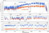 |
Fig. 1 CRIRES+ J-band spectra of the Luhman 16 binary. Top panel: nine spectral orders covered in the J1226 wavelength setting. The two reddest order-detector pairs are omitted, as explained in Sect. 2.1. Lower panels: zoomed-in view showing the similar absorption features of the two brown dwarfs. |
2.2.2 Surface gravity
The orbit of Luhman 16AB has been extensively studied (e.g. Bedin et al. 2017; Garcia et al. 2017; Lazorenko & Sahlmann 2018; Bedin et al. 2024), resulting in well-constrained dynamical masses for both components. By imposing this information as prior constraints, we can break the degeneracy that retrieval studies frequently find between the surface gravity and metallicity (e.g. Zhang et al. 2021, 2023; de Regt et al. 2024; González Picos et al. 2024). The surface gravity is related to the brown dwarf mass, M, and radius, R, via
![Mathematical equation: $\[g=\frac{G M}{R^2},\]$](/articles/aa/full_html/2025/04/aa53190-24/aa53190-24-eq11.png) (8)
(8)
with G the gravitational constant. We adopted masses of MA = 35.4 ± 0.2 and MB = 29.4 ± 0.2 MJup (Bedin et al. 2024) and a radius of R = 1 ± 0.1 RJup (Biller et al. 2024). In combination, this results in Gaussian priors of log gA = 4.96 ± 0.09 and log gB = 4.88 ± 0.09 on the surface gravity.
2.2.3 Pressure-temperature profile
Akin to Zhang et al. (2023), we modelled the thermal profile by parameterising the temperature gradient ![Mathematical equation: $\[\nabla_{i}=\frac{d ~\ln~ T_{i}}{d ~\ln~ P_{i}}\]$](/articles/aa/full_html/2025/04/aa53190-24/aa53190-24-eq12.png) at five points in log-pressure space. The outer knots were set to the limits of the modelled atmospheric layers (P1 = 103 and P5= 10−5 bar), while the three intermediate knots were allowed to shift to avoid biasing the photosphere towards certain pressures (González Picos et al. 2025). The temperature gradients ∇j at each of the 50 atmospheric layers in our pRT model are obtained through linear interpolation from the values at the knots ∇i. Subsequently, the temperature at each of the layers j is calculated via
at five points in log-pressure space. The outer knots were set to the limits of the modelled atmospheric layers (P1 = 103 and P5= 10−5 bar), while the three intermediate knots were allowed to shift to avoid biasing the photosphere towards certain pressures (González Picos et al. 2025). The temperature gradients ∇j at each of the 50 atmospheric layers in our pRT model are obtained through linear interpolation from the values at the knots ∇i. Subsequently, the temperature at each of the layers j is calculated via
![Mathematical equation: $\[T_j=T_{j-1} \cdot\left(\frac{P_j}{P_{j-1}}\right)^{\nabla_j}.\]$](/articles/aa/full_html/2025/04/aa53190-24/aa53190-24-eq13.png) (9)
(9)
This parameterisation requires an anchor point for the temperature, which we determined at the central knot (i = 3). As such, we retrieved nine parameters to describe the thermal profile: five gradients ∇i=1,2,3,4,5, three pressure points Pi=2,3,4, and one temperature Ti=3. This gradient-based parameterisation is flexible but also allows for the incorporation of radiative-convective equilibrium through the chosen prior constraints, thereby avoiding the excessively steep gradients or inversions that can arise when directly retrieving the temperature (e.g. Line et al. 2015; Mollière et al. 2020; de Regt et al. 2024).
2.2.4 Clouds
The pressures and temperatures probed with our J-band spectra cover the condensation curves of several cloud species (e.g. Fe, Mg2SiO4, and MgSiO3; Visscher et al. 2010). Hence, we modelled the total opacity of a grey cloud as
![Mathematical equation: $\[\kappa_{\mathrm{cl}}(P)= \begin{cases}\kappa_{\mathrm{cl}, 0} \cdot\left(\frac{P}{P_{\mathrm{cl}, 0}}\right)^{f_{\mathrm{sed}}} & P<P_{\mathrm{cl}, 0}, \\ 0 & P \geq P_{\mathrm{cl}, 0}.\end{cases}\]$](/articles/aa/full_html/2025/04/aa53190-24/aa53190-24-eq14.png) (10)
(10)
Here, κcl,0 is the opacity at the cloud base, set by Pcl,0, and fsed governs the opacity decay above this base (Mollière et al. 2020). This simple parameterisation limits the number of free parameters and avoids assumptions about the chemical or morphological composition of cloud particles. Although defined as opacity rather than optical depth, this cloud parameterisation is comparable to the slab clouds used in the retrieval frameworks of Burningham et al. (2017) and Vos et al. (2023). We left out any wavelength-dependence as well as additional cloud layers due to the narrow wavelength extent of the J band (~0.2 μm). Test retrievals where κcl(P) was divided into a scattering and absorption component did not yield substantially different results from including the cloud only as absorption. The single-scattering albedo used in these tests, ω, also remained unconstrained. For that reason, we included κcl(P) only as an absorption opacity in this work.
2.2.5 Chemistry
We modelled the chemical abundances using a free-chemistry approach and retrieved a volume-mixing ratio (VMR) for each of the included chemical species: H2O, FeH, HF, and the alkalis Na and K. The abundance was held constant vertically, except for FeH, which is expected to condense into iron cloud particles around the probed pressures (e.g. Visscher et al. 2010). Instead, we mimicked the rapidly decreasing FeH abundance via
![Mathematical equation: $\[\operatorname{VMR}(\mathrm{FeH})(P)= \begin{cases}\operatorname{VMR}(\mathrm{FeH})_0\left(\frac{P}{P_{\mathrm{FeH}, 0}}\right)^{\alpha_{\mathrm{FeH}}} & P<P_{\mathrm{FeH}, 0}, \\ \operatorname{VMR}(\mathrm{FeH})_0 & P \geq P_{\mathrm{FeH}, 0},\end{cases}\]$](/articles/aa/full_html/2025/04/aa53190-24/aa53190-24-eq15.png) (11)
(11)
where VMR(FeH)0 is the FeH abundance of the lower atmosphere, PFeH,0 is the pressure above which the abundance falls of with a power law, determined by αFeH. Sodium (Na) and potassium (K) should also form clouds (Na2S(s,l), KCl(s,l), and KAlSi3O8(s); Kitzmann et al. 2024), but at higher altitudes so we decided to not adopt the same rainout treatment to minimise the number of free parameters. The abundance of He is set to VMR(He) = 0.15 and that of H2 is adjusted to ensure a total mixing ratio equal to unity. Other species (e.g. CrH, TiO, VO, CH4, NH3, and Fe) were included in test retrievals but did not yield reasonable constraints on the abundances and we therefore omitted them from the presented analysis.
2.3 Opacity cross-sections
Our pRT model accounts for several sources of opacity, including collision-induced absorption from H2-H2 and H2-He pairs as well as Rayleigh scattering from H2 and He, the most abundant chemical species in a substellar atmosphere. For the molecular opacities of H2O (Polyansky et al. 2018), FeH (Dulick et al. 2003; Bernath 2020), and HF (Li et al. 2013; Coxon & Hajigeorgiou 2015; Somogyi et al. 2021), we used tables that are pre-computed on a grid of pressures and temperatures3. The perturbations brought on by collisions with H2 and He are most apparent for the strong Na and K lines. As such, we employed a more detailed treatment for the alkali opacity cross-sections.
2.3.1 Parameterised widths and shifts for the K 4p – 5s doublet
In addition to broadening the line profiles, collisions with H2 and He perturb the energy potential of the radiator thus resulting in wavelength-shifts of the line centres. The impact theories of pressure broadening (Baranger 1958; Kolb & Griem 1958) are based on the assumption of sudden collisions between the radiator and perturbing atoms, and are valid when frequency displacements and gas densities are sufficiently small. In impact broadening, the duration of the collision is assumed to be small compared to the interval between collisions, and the results describe the line within a few line widths of the centre.
We used the unified line shape theory of Allard et al. (1999), which incorporates more accurate potentials than van der Waals approximations, to determine the line parameters of the cores of the 1250 nm K doublet, perturbed by H2 and He. These lines are formed from the 4p2P3/2 − 5s (ν0 = 7983.7 cm−1) and 4p2P1/2 − 5s (ν0 = 8041.4 cm−1) transitions. For K–He, the molecular-structure calculations performed by Pascale (1983) are used for the adiabatic potential of the 5 s state and we used a combination of ab initio potentials of Santra & Kirby (2005) and Nakayama & Yamashita (2001) for the 4 p state (see Allard et al. 2024). Molecular data for the 4 p and 5 s states of K–H2 are described in Allard et al. (2016). An average over velocity was done numerically by performing the calculation for different velocities and then thermally averaging with 24-point Gauss-Laguerre integration. This impact approximation can be used to determine the line core for H2 or He densities below np = 1019 cm−3.
The determined line widths and shifts are presented in Fig. 2 as crosses and circles for a range of temperatures, for both lines, and for H2 and He perturbers. The line width, γW, is measured by half the full width at half the maximum intensity, what is customarily termed the HWHM. The solid and dashed lines in Fig. 2 show the power-law fits, defined as
![Mathematical equation: $\[\gamma_W\left[\mathrm{cm}^{-1}\right]=\sum_{p \in\left\{\mathrm{H}_2, \mathrm{He}\right\}} A_{W, p} T^{b_{W, p}}\left(\frac{n_p}{10^{20} \mathrm{~cm}^{-3}}\right),\]$](/articles/aa/full_html/2025/04/aa53190-24/aa53190-24-eq16.png) (12)
(12)
![Mathematical equation: $\[d\left[\mathrm{cm}^{-1}\right]=\sum_{p \in\left\{\mathrm{H}_2, \mathrm{He}\right\}} A_{d, p} T^{b_{d, p}}\left(\frac{n_p}{10^{20} \mathrm{~cm}^{-3}}\right).\]$](/articles/aa/full_html/2025/04/aa53190-24/aa53190-24-eq17.png) (13)
(13)
Here, d is the wavenumber-shift to be added to the line centre ν0, and np is the number density of the perturber (Allard et al. 2023). The widths and shifts are thus linearly dependent on H2/He densities, and a power law in temperature described by the AW/d and bW/d coefficients. The perturber-specific coefficients for both transitions are given in Table 1. Utilising these parameters results in blueshifted line profiles with increasing pressures, as is demonstrated for the 4p2P3/2 − 5s line in Fig. 3.
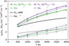 |
Fig. 2 Variation with temperature of the broadening (γW/np, solid) and shift (d/np, dashed) rates of the 4p2P3/2 − 5s (green) and 4p2P1/2 − 5s (purple) lines, perturbed by H2 and He. The van der Waals (vdW) broadening, computed with Eq. (16), is shown in black for comparison. |
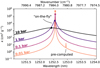 |
Fig. 3 Opacity cross-sections for potassium (K) at T = 1500 K. The weak line at 1252.95 nm is interpolated from a pre-computed opacity table. The doublet line at 1252.55 nm (4p2P3/2 − 5s) is computed ‘on-the-fly’, meaning that the line strength and line width are calculated exactly for each PT point in the modelled atmosphere. This line also receives a PT-dependent shift, resulting in a blueshift at high pressures. |
2.3.2 ’On-the-fly’ line profiles
During the retrieval, pRT interpolates the pre-computed molecular cross-section of H2O, FeH, and HF onto the pressures and temperatures of the model atmospheres. This conventional interpolation method bypasses calculating thousands of line profiles at each of the atmospheric layers, thereby drastically reducing the computation time. However, we find that the nominal pressure-spacing of 1 dex is too sparse to properly fit the strongly pressure-broadened Na and K doublets (see Sect. 4.2). Since there are few strong alkali lines in the J-band wavelength range, it is computationally feasible to use a more exact method to obtain their opacities.
We acquired energy, oscillator-strength, and broadening information from the Kurucz4 and National Institute of Standards and Technology (NIST) databases5 for neutral Na and K (Kurucz 2018). During the retrieval, we interpolated the opacity from weak lines (with oscillator strengths log g f < −0.5) from a pre-computed table. Stronger lines were calculated ‘on-the-fly’ at the temperature and pressure of each atmospheric layer, resulting in accurate thermal- and pressure-broadening prescriptions. We implemented these opacities using the additional_absorption_opacities_function functionality in pRT. Following Sharp & Burrows (2007) and Gandhi et al. (2020), we defined the Gaussian and Lorentzian half-widths as
![Mathematical equation: $\[\gamma_G\left[\mathrm{cm}^{-1}\right]=\frac{v_0}{c} \sqrt{\frac{2 k_B T}{m_X}},\]$](/articles/aa/full_html/2025/04/aa53190-24/aa53190-24-eq18.png) (14)
(14)
![Mathematical equation: $\[\gamma_L\left[\mathrm{cm}^{-1}\right]=\gamma_N+\sum_{p \in\left\{\mathrm{H}_2, \mathrm{He}\right\}} \gamma_{W, p},\]$](/articles/aa/full_html/2025/04/aa53190-24/aa53190-24-eq19.png) (15)
(15)
where ν0 is the transition energy, mX the atomic mass of Na or K (in g), and γN the natural broadening, which is negligible at the high pressures of the Luhman 16 photospheres. For all but the K 4p − 5s lines, we calculated the half-width per perturber following Eq. (23) in Sharp & Burrows (2007):
![Mathematical equation: $\[\gamma_{W, p}\left[\mathrm{cm}^{-1}\right]=\frac{\gamma_{\mathrm{vdW}}^{\mathrm{Kurucz}}}{4 \pi c}\left(\frac{\mu_{\mathrm{H}, X}}{\mu_{p, X}} \frac{T}{10~000 \mathrm{~K}}\right)^{3 / 10}\left(\frac{\alpha_p}{\alpha_{\mathrm{H}}}\right)^{2 / 5} \cdot n_p,\]$](/articles/aa/full_html/2025/04/aa53190-24/aa53190-24-eq20.png) (16)
(16)
where ![Mathematical equation: $\[\gamma_{\mathrm{vdW}}^{\mathrm{Kurucz}}\]$](/articles/aa/full_html/2025/04/aa53190-24/aa53190-24-eq21.png) is the van der Waals coefficient provided in the Kurucz line list, μa,b = mamb/(ma + mb) is the reduced mass (in g), and αa is the polarisability of species a (in cm3). The black (H2) and grey (He) lines in Fig. 2 show the broadening rates calculated with Eq. (16) for the K 4p − 5s transitions. The Kurucz line list reports the same
is the van der Waals coefficient provided in the Kurucz line list, μa,b = mamb/(ma + mb) is the reduced mass (in g), and αa is the polarisability of species a (in cm3). The black (H2) and grey (He) lines in Fig. 2 show the broadening rates calculated with Eq. (16) for the K 4p − 5s transitions. The Kurucz line list reports the same ![Mathematical equation: $\[\gamma_{\mathrm{vdW}}^{\mathrm{Kurucz}}=10^{-7.46} \mathrm{~s}^{-1} \mathrm{~cm}^{3}\]$](/articles/aa/full_html/2025/04/aa53190-24/aa53190-24-eq22.png) for both lines. Figure 2 reveals that the van der Waals approximation would underpredict the pressure broadening compared to the method outlined in Sect. 2.3.1.
for both lines. Figure 2 reveals that the van der Waals approximation would underpredict the pressure broadening compared to the method outlined in Sect. 2.3.1.
3 Results
Our fiducial model provides a good fit to the Luhman 16 binary spectra, as presented for one spectral order in Fig. 4. The full wavelength coverage is found in Appendix C. The residuals mostly fall within the expected uncertainties (shown as error bars), which are inflated during the fitting by a factor of ![Mathematical equation: $\[\tilde{s}^{2} \sim 1.2-1.5\]$](/articles/aa/full_html/2025/04/aa53190-24/aa53190-24-eq23.png) to obtain a reduced χ2 equal to unity (see e.g. Ruffio et al. 2019; Gibson et al. 2020). We suspect that the minor model deficiencies (e.g. ~1192–1196, 1211, 1281, 1292, 1319–1324, and 1334 nm) arise due to missing absorbers or inaccuracies in the utilised line lists. Including other molecular or atomic species (e.g. CrH, TiO, VO, CH4, NH3, and Fe), however, did not improve the fit or produce reasonable constraints on the abundances.
to obtain a reduced χ2 equal to unity (see e.g. Ruffio et al. 2019; Gibson et al. 2020). We suspect that the minor model deficiencies (e.g. ~1192–1196, 1211, 1281, 1292, 1319–1324, and 1334 nm) arise due to missing absorbers or inaccuracies in the utilised line lists. Including other molecular or atomic species (e.g. CrH, TiO, VO, CH4, NH3, and Fe), however, did not improve the fit or produce reasonable constraints on the abundances.
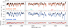 |
Fig. 4 Best-fitting models to the J-band spectra of Luhman 16. The observations are shown in black, while the fiducial models are shown in orange and blue for Luhman 16A and B, respectively. The mean scaled uncertainties, defined as diag ( |
![Mathematical equation: $\[\tilde{s}_{i} \sqrt{\Sigma_{0, i}}\right\]$](/articles/aa/full_html/2025/04/aa53190-24/aa53190-24-eq24.png)
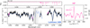 |
Fig. 5 Detection analysis of HF in the Luhman 16B spectrum. The left panels show the spectral contribution of HF by comparing the complete model (solid blue line) to a model without HF (dashed pink line). The residuals show the difference between these two models. The right panel presents the CCF described in Sect. 3.1. |
3.1 Detection of chemical species
From a visual inspection, we identified lines from H2O, K and Na in the spectra of both brown dwarfs. As noted by Faherty et al. (2014) and Lodieu et al. (2015), the Na doublet at ~1140 nm is weak and contaminated by (telluric) H2O absorption, but is definitely present in our CRIRES+spectra (see Fig. 1). The 1250 nm K doublet of Luhman 16B shows stronger absorption compared to the primary, in line with previous studies covering the J band (Burgasser et al. 2013; Faherty et al. 2014; Lodieu et al. 2015). Contrary to Faherty et al. (2014) and Lodieu et al. (2015), we do not detect CH4 with the up-to-date ExoMol line list (Yurchenko et al. 2024). This discrepancy might result from a fluctuation in the disequilibrium chemistry, where CH4 would play a role (e.g. Zahnle & Marley 2014; Lee et al. 2024), but a comparison with the X-SHOOTER data of Lodieu et al. (2015) revealed no major spectral differences.
We detect hydrogen-fluoride (HF) and iron-hydride (FeH) in the atmospheres of Luhman 16. The left panels in Figs. 5 and 6 show examples of the contributed absorption from HF and FeH, respectively. The inclusion of either molecule results in a closer match to the observed spectrum of Luhman 16B. To assess the detection significance further, we carried out a cross-correlation analysis between the residuals of a model without species X (mi,w/o X) and a template that only includes lines from the tested species (mi,only X). The total cross-correlation function (CCF), at a velocity v, is then summed over each chip i via
![Mathematical equation: $\[\operatorname{CCF}(\nu)=\sum_i \frac{1}{\tilde{s}_i^2}\left(\boldsymbol{d}_i-\tilde{\phi} \boldsymbol{m}_{i, \mathrm{w} / \mathrm{o} X}\right)^T \boldsymbol{\Sigma}_{0, i}^{-1} ~\boldsymbol{m}_{i, \text { only } X}(\nu).\]$](/articles/aa/full_html/2025/04/aa53190-24/aa53190-24-eq25.png) (17)
(17)
The right panels of Figs. 5 and 6 display this CCF, normalised to a signal-to-noise function using samples outside of the peak (|v| > 300 km s−1). For Luhman 16B, the cross-correlation yields peak detection significances of 6.7 and 8.5σ for HF and FeH, respectively. The detection significances for Luhman 16A are 5.1 and 10.7σ, respectively, for HF and FeH (see Appendix D). The FeH absorption in the J-band spectra of Luhman 16AB was identified previously by Faherty et al. (2014). To our knowledge, HF has not been detected in the J-band spectrum of any substellar object. However, recent studies have identified its spectral signature in the K band (González Picos et al. 2024; Zhang et al. 2024; Mulder et al. 2025) and we provide a discussion in the analysis of the Luhman 16 K-band spectra (de Regt et al., in prep.).
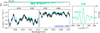 |
Fig. 6 Same as Fig. 5 but for FeH. The model spectrum without FeH is shown as the dashed turquoise line. |
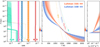 |
Fig. 7 Retrieved vertical profiles of Luhman 16A (solid) and Luhman 16B (dashed). Left panel: chemical abundances and the 68, 95, and 99.7% confidence envelopes of each species for both brown dwarfs. The dotted lines show the chemical-equilibrium abundances computed with FastChem (Kitzmann et al. 2024). With the exception of FeH, the modelled abundances are constant with altitude and thus do not show the drop-offs exhibited by the equilibrium profiles. Middle panel: inferred temperature profiles and the condensation curves (dotted) of four cloud species (Visscher et al. 2006, 2010). Right panel: grey-cloud opacities retrieved as a function of altitude. The orange and blue shading in the panel gaps indicate the Luhman 16AB photospheres as obtained with the integrated emission contribution functions. |
3.2 Chemical abundances
The left panel of Fig. 7 shows the retrieved abundance profiles of Luhman 16A and B as solid and dashed lines, respectively. The two brown dwarfs display remarkably similar abundances, which agree to within ~3σ for all species except FeH. The dotted lines in the left panel of Fig. 7 indicate the expected chemical-equilibrium abundances, computed using the FastChem code (Kitzmann et al. 2024). As input, we accounted for rainout condensation and assumed a solar composition (i.e. [Fe/H] = 0, C/O = 0.59; Asplund et al. 2021). For the most part, the equilibrium abundances of H2O and HF are constant with altitude and in accordance with our retrieved abundances. The equilibrium profiles of Na and K show a drop-off in the gaseous abundance beyond ~0.3 bar as a result of rainout into sodium- and potassium-bearing condensate species. Our retrieved photospheres are located between ~0.6 and 11 bar, as indicated in the panel gaps, and therefore probe largely constant abundances below this drop-off. We find super-solar alkali abundances where the inferred Na abundance appears elevated by ~0.5 dex, despite the weak absorption seen in Fig. 1.
3.3 Clouds and condensation
The middle panel of Fig. 7 presents the retrieved temperature profiles of Luhman 16A and B as solid orange and dashed blue lines, respectively. In addition, the dotted condensation curves demonstrate the conditions under which the corresponding clouds should form, assuming a solar composition (Visscher et al. 2006, 2010). The right panel of Fig. 7 reveals the grey-cloud opacities retrieved for both brown dwarfs. It is interesting to note that the temperature and cloud profiles differ between Luhman 16A and B, whereas the chemical abundances of HF, K, Na, and H2O are in good agreement. This possibly indicates a warming effect by more vertically extended clouds on Luhman 16A (e.g. Morley et al. 2024). The cloud base pressures (![Mathematical equation: $\[P_{\mathrm{cl}, 0, \mathrm{A}}=13.3_{-1.2}^{+1.3}, P_{\mathrm{cl}, 0, \mathrm{B}}=18.3_{-1.1}^{+1.4} ~\mathrm{bar}\]$](/articles/aa/full_html/2025/04/aa53190-24/aa53190-24-eq26.png) ) coincide with the intersection between the silicate-oxide (MgSiO3 and Mg2SiO4) condensation curves and the retrieved pressure-temperature (PT) profiles. These silicate clouds in the Luhman 16AB atmospheres seemingly weaken the J-band spectral features, particularly those formed at high pressures.
) coincide with the intersection between the silicate-oxide (MgSiO3 and Mg2SiO4) condensation curves and the retrieved pressure-temperature (PT) profiles. These silicate clouds in the Luhman 16AB atmospheres seemingly weaken the J-band spectral features, particularly those formed at high pressures.
The condensation curve of iron (Visscher et al. 2010) intersects with the Luhman 16AB temperature profiles below the photospheric regions. Iron-bearing species are thus expected to rain out at higher altitudes, thereby decreasing their gaseous abundances. This abundance decrease is also apparent from the equilibrium profile of FeH (dotted turquoise line) in the left panel of Fig. 7. The FeH abundance of Luhman 16A (solid turquoise line) shows a constraint on a depletion near ~5 bar, although it does not perfectly follow the equilibrium prediction. Conversely, we retrieve FeH at a constant abundance for Luhman 16B (dashed turquoise line). The drop-off pressure for this secondary component is constrained to be above the photospheric altitudes, which leaves the modelled spectrum unaltered. In both brown dwarfs, we find evidence of a higher, non-equilibrium abundance of FeH within the photosphere.
3.4 Two-column model
If regions of thinner clouds have formed within the Luhman 16AB photospheres, this could expose deeper, hotter layers of their atmospheres (Faherty et al. 2014). Our measured elevated FeH abundances might correspond with such clearer patches, similar to the reasoning given for the FeH re-emergence in early T-type brown dwarfs (Burgasser et al. 2002). We tested this hypothesis by introducing a two-column model akin to Buenzli et al. (2015) and Vos et al. (2023). The two columns share most parameters (e.g. PT profile, chemistry, and log g), but have distinct FeH abundances and cloud opacities. The total flux is obtained by summing the separate fluxes, Fi, while accounting for 𝒞ℱ, the surface coverage fraction,
![Mathematical equation: $\[F_{\text {tot }}=\mathcal{CF} \cdot F_1+(1-\mathcal{CF}) \cdot F_2.\]$](/articles/aa/full_html/2025/04/aa53190-24/aa53190-24-eq27.png) (18)
(18)
Thus, an equivalent to the one-column solution can be achieved by setting 𝒞ℱ = 1 (or 0) and retrieving the same parameters for column 1 (or column 2). The additional FeH-abundance, cloud-opacity and coverage parameters increase the number of retrieval parameters from 25 to 32 in the two-column model.
Modelling the Luhman 16A atmosphere as a combination of two columns results in constraints on opaque clouds in both patches (see Table B.1). The smaller patch covers ~6% of the surface and hosts a cloud deck below that of the larger patch (![Mathematical equation: $\[P_{\mathrm{cl}, 0}=35.9_{-6.6}^{+8.8}\]$](/articles/aa/full_html/2025/04/aa53190-24/aa53190-24-eq28.png) and
and ![Mathematical equation: $\[9.8_{-0.9}^{+1.1} ~\mathrm{bar}\]$](/articles/aa/full_html/2025/04/aa53190-24/aa53190-24-eq29.png) ). In addition, the minor column finds a constant-with-altitude abundance for FeH (
). In addition, the minor column finds a constant-with-altitude abundance for FeH (![Mathematical equation: $\[-7.95_{-0.08}^{+0.11}\]$](/articles/aa/full_html/2025/04/aa53190-24/aa53190-24-eq30.png) ), in contrast to the other, FeH-depleted column. Despite these constraints, a Bayesian evidence comparison reveals that the two-column retrieval is not favoured over the single column (ln B = −13.3; ~5.5σ) due to the increased model complexity.
), in contrast to the other, FeH-depleted column. Despite these constraints, a Bayesian evidence comparison reveals that the two-column retrieval is not favoured over the single column (ln B = −13.3; ~5.5σ) due to the increased model complexity.
For Luhman 16B, the Bayesian evidence shows a marginal preference for a two-column solution compared to a single column (ln B = 0.67; ~1.8σ). However, the constrained parameters are not substantially different from the one-column retrieval. The cloud deck of the one-column solution is replicated by a dominant column that accounts for ~98% of the flux (see Table B.1). The distinct surface gravities constrained in both retrievals hinders a direct comparison of the abundances due to a log g-metallicity degeneracy (Zhang et al. 2021, 2023; de Regt et al. 2024; González Picos et al. 2024). Nevertheless, the dominant column seemingly adopts the equivalent FeH abundance (![Mathematical equation: $\[-9.26_{-0.08}^{+0.07}\]$](/articles/aa/full_html/2025/04/aa53190-24/aa53190-24-eq31.png) ) of the one-column retrieval (
) of the one-column retrieval (![Mathematical equation: $\[-8.90_{-0.06}^{+0.05}\]$](/articles/aa/full_html/2025/04/aa53190-24/aa53190-24-eq32.png) ). The minor patch, which covers only ~2% of the modelled surface, hosts no significant cloud opacity and therefore results in a deeper photosphere. At these higher pressures, the retrieval constrains an elevated FeH abundance (
). The minor patch, which covers only ~2% of the modelled surface, hosts no significant cloud opacity and therefore results in a deeper photosphere. At these higher pressures, the retrieval constrains an elevated FeH abundance (![Mathematical equation: $\[-7.97_{-0.09}^{+0.10}\]$](/articles/aa/full_html/2025/04/aa53190-24/aa53190-24-eq33.png) ).
).
4 Discussion
4.1 Surface (in)homogeneity
The Luhman 16A spectrum is best described with a single-column model, which points towards a relatively homogeneous surface. This conclusion aligns well with the reduced variability observed for the primary (~2%; Biller et al. 2024) as well as the weak features inferred in Doppler imaging analyses (Crossfield et al. 2014; Chen et al. 2024). Given its L7.5 spectral type, it is perhaps not surprising that the cloud dissipation expected at the L–T transition has not commenced (Burgasser et al. 2002; Marley et al. 2010). On the other hand, the marginally preferred two-column model for Luhman 16B (~1.8σ) constitutes a more ambiguous result. We caution that the constrained coverage fraction, clouds, and FeH abundances are likely biased due to assumptions made to reduce the number of free parameters in the two-column retrieval. For instance, we adopted the same temperature profile for both columns, despite the heating that should result from the radiative feedback of an opaque cloud (Tan & Showman 2019, 2021a,b). In turn, the altered thermal profile will affect the atmospheric chemistry (Lee et al. 2023, 2024), which challenges our choice of shared abundances between the two columns. Introducing more parameters to describe separate columns of emission, however, will likely lead to issues of convergence or over-fitting instead of resolving the mentioned ambiguity. Rather, observations over a broader wavelength-range could help probe the vertical extent of FeH (e.g. in the Y, J, and H bands; Faherty et al. 2014) and the presence of clouds at different altitudes (Vos et al. 2023).
4.2 Alkali line asymmetry
The potassium doublet near 1250 nm shows an asymmetry in both lines, for both brown dwarfs. Figure 8 presents an analysis of the potassium absorption lines for Luhman 16B. The red model demonstrates the unsatisfactory fit obtained when only considering van der Waals broadening and ignoring line-shifts. It is evident from the right panel of Fig. 8 that the model profiles, centred on the dotted lines, cannot fit the excess absorption in the blue wing of the lines. The retrieval attempts to alter the photospheric pressures via the surface gravity, temperature profile and cloud deck, resulting in a worsened fit to the bluer J-band doublet (left panel) as well. The model in green utilises pre-computed opacities, calculated on the default 1 dex pressure-spacing of petitRADTRANS (Mollière et al. 2019). These opacity cross-sections employ the width- and shift-parameterisation of Sect. 2.3.1, but not necessarily at the atmospheric conditions encountered in the Luhman 16 photospheres. This modelling approach results in a better fit to the line wings, but cannot reproduce the line cores adequately. In addition, we find that the model deviates for the other strong alkali lines (left panel) as a result of the interpolation.
The ‘on-the-fly’ opacity calculation outlined in Sect. 2.3.2 results in the best-fitting model, shown in blue in Fig. 8. The residuals of the 1175 nm K doublet are minimised, but even this involved opacity treatment fails to completely reproduce the 1250 nm profiles. Several factors could contribute to this deviation. First, the line profiles will become non-Lorentzian for perturber densities ≳1019 cm−3, akin to the optical resonance lines (Allard et al. 2016, 2024). Our deepest photospheric layers achieve H2 densities of nH2 ~ 3 × 1019 cm−3, thus challenging the validity of the utilised approach. Furthermore, the assumed H2/He abundance ratio affects the total broadening and shift applied to both lines. In the future, using high-resolution spectra with sufficient signal-to-noise ratios, one could attempt to infer the H2 and He abundances from the detected line-shifts and – widths. However, since degenerate solutions will likely arise, this is beyond the scope of this study. Additionally, the vertically constant abundance employed for potassium could overestimate the opacity at altitudes where rainout occurs. However, this implies that the current model line core is too deep, contrary to what is seen in Fig. 8.
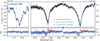 |
Fig. 8 Potassium absorption lines of Luhman 16B modelled with different approaches. Left panel: strong 4p2P3/2 − 3d2D3/2 and 4p2P3/2 − 3d2D5/2 transitions at the blue end of the J band. Right panel: 4p − 5s doublet showing asymmetries compared to the expected transition wavelengths, indicated with dotted lines. |
5 Conclusions
We performed an atmospheric analysis of the nearest brown dwarfs, Luhman 16AB, using high-resolution J-band spectra taken with CRIRES+. The brightness of the two targets provides an unprecedented level of detail for substellar objects. Our petitRADTRANS retrieval models can account for almost all the spectral features present in the J band. Minor deficiencies likely arise from missing absorbers or inaccuracies in the current line lists. These high-quality, high-resolution spectra can form a testbed when updated line lists become available.
For both brown dwarfs, we detect absorption from H2O, K, Na, HF, and FeH. For the first time, this work presents an HF detection in the J-band spectrum of a substellar atmosphere. The retrieval constrains Na (and K) at super-equilibrium abundances despite the weak doublet absorption at ~1140 nm (Faherty et al. 2014; Lodieu et al. 2015). We find evidence of opaque clouds in the Luhman 16AB photospheres, which are likely made up of silicate-oxide condensates given the constrained cloud deck pressure. The Luhman 16A spectrum is best fit with a homogeneous surface model that includes an FeH depletion, in line with its reduced variability and L7.5 spectral type (Burgasser et al. 2013; Buenzli et al. 2015; Biller et al. 2024). We constrain over-abundant FeH in the photosphere of Luhman 16B, which is at odds with the expected condensation into iron clouds. Modelling the Luhman 16B surface as a combination of cloudy and clear patches, however, leads to ambiguous results as this two-column solution is only favoured at ~1.8σ compared to a homogeneous surface. Observations spanning a wider wavelength range, with JWST for instance, can aid in resolving the altitude-dependent abundance of FeH as well as the vertical extent of cloud decks.
We detect asymmetric absorption in the 1250 nm potassium doublet lines (4p − 5s) of Luhman 16AB. Employing the unified line shape theory of Allard et al. (1999), we parameterised the PT-dependent widths and shifts of the Lorentzian profiles. The blueshifted absorption excess can mostly be reproduced via this careful modelling approach, but the degeneracy with metallicity hinders surface-gravity measurements from our high-resolution spectra alone. Future high-resolution observations of asymmetric atomic lines could help us understand the perturber physics in the substellar and low-mass regime.
The ESO SupJup Survey observations were mostly taken in the K band, where the C/O ratio and carbon isotopes can be measured. In that context, the presented analysis provides access to elements that lack absorption features in the K band for these temperatures, such as Na, K, and Fe. The higher pressures probed in the J band also permit the investigation of cloud structures. Thus, high-resolution J-band spectra offer valuable insights into the atmospheric properties of Luhman 16AB in particular, and brown dwarfs in general.
Acknowledgements
We thank the anonymous referee for their constructive comments. S.d.R. and I.S. acknowledge funding from NWO grant OCENW.M.21.010. Based on observations collected at the European Organisation for Astronomical Research in the Southern Hemisphere under ESO programme(s) 110.23RW.002. This work used the Dutch national e-infrastructure with the support of the SURF Cooperative using grant no. EINF-4556 and EINF-9460. This research has made use of the Astrophysics Data System, funded by NASA under Cooperative Agreement 80NSSC21M00561. Software: Astropy (Astropy Collaboration 2022), corner (Foreman-Mackey 2016), FastChem (Kitzmann et al. 2024), Matplotlib (Hunter 2007), NumPy (Harris et al. 2020), petitRADTRANS (Mollière et al. 2019), PyAstronomy (Czesla et al. 2019), PyMultiNest (Feroz et al. 2009; Buchner et al. 2014), SciPy (Virtanen et al. 2020).
Appendix A Contamination correction
Figure A.1 demonstrates the spectral contamination between components A and B for a single chip. The left panel displays the two-dimensional spectrum where the slit tilt and slit curvature are rectified in the excalibuhr-reduction. The upper and lower traces are the emission of Luhman 16B and A, respectively. The spatial profile, median-combined over all wavelength channels in the chip, is shown in black in the right panel of Fig. A.1. While the peak emissions can be distinguished at a separation of ~0.81” (as predicted by Bedin et al. 2024), there exists ~6–11% contamination within the respective 12-pixel wide extraction apertures.
To correct the contamination, we fitted two Moffat functions6 to the observed spatial profile. These fitted profiles, ΦA and ΦB, are shown in orange and blue, respectively, in the right panel of Fig. A.1. The profiles are subsequently integrated over the extraction apertures to assess the relative contributions. The measured flux in aperture A is then the weighted sum of the uncontaminated total fluxes of components A and B. That is,
![Mathematical equation: $\[F_{\text {in aper.} \mathrm{A}}=\left(\frac{\int_{\text {aper.} \mathrm{A}} \Phi_{\mathrm{A}}}{\int \Phi_{\mathrm{A}}}\right) \cdot F_{\text {tot}, \mathrm{A}}+\left(\frac{\int_{\text {aper.} \mathrm{A}} \Phi_{\mathrm{B}}}{\int \Phi_{\mathrm{B}}}\right) \cdot F_{\text {tot,} \mathrm{B}},\]$](/articles/aa/full_html/2025/04/aa53190-24/aa53190-24-eq34.png) (A.1)
(A.1)
where the integrals over aperture A are normalised by integrals over the complete profiles. Similarly, the measured flux in aperture B is expressed as
![Mathematical equation: $\[F_{\text {in aper.} ~\mathrm{B}}=\left(\frac{\int_{\text {aper.} \mathrm{B}} \Phi_{\mathrm{A}}}{\int \Phi_{\mathrm{A}}}\right) \cdot F_{\text {tot}, \mathrm{A}}+\left(\frac{\int_{\text {aper.} \mathrm{B}} \Phi_{\mathrm{B}}}{\int \Phi_{\mathrm{B}}}\right) \cdot F_{\text {tot}, \mathrm{B}}.\]$](/articles/aa/full_html/2025/04/aa53190-24/aa53190-24-eq35.png) (A.2)
(A.2)
Through substitution, we obtain definitions for the blending-corrected fluxes of Luhman 16A and B,
![Mathematical equation: $\[F_{\mathrm{A}}=F_{\text {in aper. } \mathrm{A}}-\left(\frac{\int_{\text {aper. } \mathrm{A}} \Phi_{\mathrm{B}}}{\int_{\text {aper. } \mathrm{B}} \Phi_{\mathrm{B}}}\right) \cdot F_{\text {in aper. } \mathrm{B}},\]$](/articles/aa/full_html/2025/04/aa53190-24/aa53190-24-eq36.png) (A.3)
(A.3)
![Mathematical equation: $\[F_{\mathrm{B}}=F_{\text {in aper. } \mathrm{B}}-\left(\frac{\int_{\text {aper. } \mathrm{B}} \Phi_{\mathrm{A}}}{\int_{\text {aper. } \mathrm{A}} \Phi_{\mathrm{A}}}\right) \cdot F_{\text {in aper. A}}.\]$](/articles/aa/full_html/2025/04/aa53190-24/aa53190-24-eq37.png) (A.4)
(A.4)
We note that FA ≠ Ftot,A (and FB ≠ Ftot,B) because a scaling factor is omitted. The absolute scale of FA (and FB), however, is not important because the spectrum is flux-calibrated after the outlined contamination correction (see Sect. 2.1). The seeing-limited point-spread function becomes narrower at longer wavelengths, and we therefore performed the correction separately for each chip.
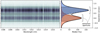 |
Fig. A.1 Assessment of the spectral blending in the 23rd chip (centred at ~1312 nm). Left panel: Two-dimensional spectrum, showing emission from Luhman 16B and A at the top and bottom, respectively. The vertical lines show the strong absorption from tellurics. Right panel: Median spatial profile (black) along with fitted Moffat functions, ΦA (orange) and ΦB (blue). The flux within the 12-pixel-wide extraction apertures includes contamination from the unwanted binary component. |
Appendix B Retrieved parameters
Retrieved parameters and their uncertainties.
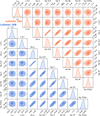 |
Fig. B.1 Posterior distributions of a selection of parameters for the Luhman 16AB one-column retrievals. For both objects, we find a strong correlation between the surface gravity, log g, and the abundances. However, the retrieved surface gravities do not deviate from the imposed Gaussian priors, which implies that the constrained abundances are accurate. The radial velocity, vrad, shows no correlation and could therefore help constrain the Luhman 16AB orbits further. |
Appendix C Best-fitting spectra
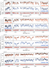 |
Fig. C.1 Same as Fig. 4 but showing all spectral orders. The missing spectral order is shown in Fig. 4. |
Appendix D HF and FeH detection on Luhman 16A
References
- Ackerman, A. S., & Marley, M. S. 2001, ApJ, 556, 872 [Google Scholar]
- Alei, E., Konrad, B. S., Angerhausen, D., et al. 2022, A&A, 665, A106 [NASA ADS] [CrossRef] [EDP Sciences] [Google Scholar]
- Allard, N. F., Royer, A., Kielkopf, J. F., & Feautrier, N. 1999, Phys. Rev. A, 60, 1021 [Google Scholar]
- Allard, N. F., Kielkopf, J. F., & Allard, F. 2007, Eur. Phys. J. D, 44, 507 [NASA ADS] [CrossRef] [Google Scholar]
- Allard, N. F., Spiegelman, F., & Kielkopf, J. F. 2016, A&A, 589, A21 [NASA ADS] [CrossRef] [EDP Sciences] [Google Scholar]
- Allard, N. F., Myneni, K., Blakely, J. N., & Guillon, G. 2023, A&A, 674, A171 [NASA ADS] [CrossRef] [EDP Sciences] [Google Scholar]
- Allard, N. F., Kielkopf, J. F., Myneni, K., & Blakely, J. N. 2024, A&A, 683, A188 [NASA ADS] [CrossRef] [EDP Sciences] [Google Scholar]
- Allers, K. N., & Liu, M. C. 2013, ApJ, 772, 79 [NASA ADS] [CrossRef] [Google Scholar]
- Arcos, C., Kanaan, S., Chávez, J., et al. 2018, MNRAS, 474, 5287 [NASA ADS] [CrossRef] [Google Scholar]
- Artigau, E., Bouchard, S., Doyon, R., & Lafrenière, D. 2009, ApJ, 701, 1534 [NASA ADS] [CrossRef] [Google Scholar]
- Asplund, M., Amarsi, A. M., & Grevesse, N. 2021, A&A, 653, A141 [NASA ADS] [CrossRef] [EDP Sciences] [Google Scholar]
- Astropy Collaboration (Price-Whelan, A. M., et al.) 2022, ApJ, 935, 167 [NASA ADS] [CrossRef] [Google Scholar]
- Baranger, M. 1958, Phys. Rev., 111, 481 [NASA ADS] [CrossRef] [Google Scholar]
- Bedin, L. R., Pourbaix, D., Apai, D., et al. 2017, MNRAS, 470, 1140 [NASA ADS] [CrossRef] [Google Scholar]
- Bedin, L. R., Dietrich, J., Burgasser, A. J., et al. 2024, Astron. Nachr., 345, e20230158 [NASA ADS] [Google Scholar]
- Bernath, P. F. 2020, J. Quant. Spec. Radiat. Transf., 240, 106687 [NASA ADS] [CrossRef] [Google Scholar]
- Biller, B. A., Crossfield, I. J. M., Mancini, L., et al. 2013, ApJ, 778, L10 [Google Scholar]
- Biller, B. A., Vos, J. M., Zhou, Y., et al. 2024, MNRAS, 532, 2207 [NASA ADS] [CrossRef] [Google Scholar]
- Buchner, J., Georgakakis, A., Nandra, K., et al. 2014, A&A, 564, A125 [NASA ADS] [CrossRef] [EDP Sciences] [Google Scholar]
- Buenzli, E., Saumon, D., Marley, M. S., et al. 2015, ApJ, 798, 127 [Google Scholar]
- Burgasser, A. J., Marley, M. S., Ackerman, A. S., et al. 2002, ApJ, 571, L151 [NASA ADS] [CrossRef] [Google Scholar]
- Burgasser, A. J., Sheppard, S. S., & Luhman, K. L. 2013, ApJ, 772, 129 [Google Scholar]
- Burningham, B., Marley, M. S., Line, M. R., et al. 2017, MNRAS, 470, 1177 [NASA ADS] [CrossRef] [Google Scholar]
- Burrows, A., Sudarsky, D., & Hubeny, I. 2006, ApJ, 640, 1063 [Google Scholar]
- Chen, X., Biller, B. A., Vos, J. M., et al. 2024, MNRAS, 533, 3114 [Google Scholar]
- Coxon, J. A., & Hajigeorgiou, P. G. 2015, J. Quant. Spec. Radiat. Transf., 151, 133 [NASA ADS] [CrossRef] [Google Scholar]
- Crossfield, I. J. M., Biller, B., Schlieder, J. E., et al. 2014, Nature, 505, 654 [NASA ADS] [CrossRef] [Google Scholar]
- Cushing, M. C., Rayner, J. T., & Vacca, W. D. 2005, ApJ, 623, 1115 [Google Scholar]
- Czesla, S., Schröter, S., Schneider, C. P., et al. 2019, PyA: Python astronomy-related packages, Astrophysics Source Code Library [record ascl:1906.010] [Google Scholar]
- de Regt, S., Gandhi, S., Snellen, I. A. G., et al. 2024, A&A, 688, A116 [NASA ADS] [CrossRef] [EDP Sciences] [Google Scholar]
- Dorn, R. J., Bristow, P., Smoker, J. V., et al. 2023, A&A, 671, A24 [NASA ADS] [CrossRef] [EDP Sciences] [Google Scholar]
- Dulick, M., Bauschlicher, C. W., J., Burrows, A., et al. 2003, ApJ, 594, 651 [NASA ADS] [CrossRef] [Google Scholar]
- Dupuy, T. J., & Liu, M. C. 2012, ApJS, 201, 19 [NASA ADS] [CrossRef] [Google Scholar]
- Faherty, J. K., Beletsky, Y., Burgasser, A. J., et al. 2014, ApJ, 790, 90 [NASA ADS] [CrossRef] [Google Scholar]
- Feroz, F., Hobson, M. P., & Bridges, M. 2009, MNRAS, 398, 1601 [NASA ADS] [CrossRef] [Google Scholar]
- Foreman-Mackey, D. 2016, J. Open Source Softw., 1, 24 [Google Scholar]
- Fuda, N., Apai, D., Nardiello, D., et al. 2024, ApJ, 965, 182 [Google Scholar]
- Gagné, J., Moranta, L., Faherty, J. K., et al. 2023, ApJ, 945, 119 [CrossRef] [Google Scholar]
- Gandhi, S., Brogi, M., Yurchenko, S. N., et al. 2020, MNRAS, 495, 224 [NASA ADS] [CrossRef] [Google Scholar]
- Garcia, E. V., Ammons, S. M., Salama, M., et al. 2017, ApJ, 846, 97 [NASA ADS] [CrossRef] [Google Scholar]
- Gibson, N. P., Merritt, S., Nugroho, S. K., et al. 2020, MNRAS, 493, 2215 [Google Scholar]
- González Picos, D., Snellen, I. A. G., de Regt, S., et al. 2024, A&A, 689, A212 [NASA ADS] [CrossRef] [EDP Sciences] [Google Scholar]
- González Picos, D., Snellen, I. A. G., de Regt, S., et al. 2025, A&A, 693, A298 [NASA ADS] [CrossRef] [EDP Sciences] [Google Scholar]
- Harris, C. R., Millman, K. J., van der Walt, S. J., et al. 2020, Nature, 585, 357 [NASA ADS] [CrossRef] [Google Scholar]
- Hunter, J. D. 2007, Comput. Sci. Eng., 9, 90 [NASA ADS] [CrossRef] [Google Scholar]
- Kirkpatrick, J. D. 2005, ARA&A, 43, 195 [NASA ADS] [CrossRef] [Google Scholar]
- Kitzmann, D., Stock, J. W., & Patzer, A. B. C. 2024, MNRAS, 527, 7263 [Google Scholar]
- Kolb, A. C., & Griem, H. 1958, Phys. Rev., 111, 514 [NASA ADS] [CrossRef] [Google Scholar]
- Kurucz, R. L. 2018, in, Workshop on Astrophysical Opacities, Astronomical Society of the Pacific Conference Series, 515, 47 [Google Scholar]
- Lazorenko, P. F., & Sahlmann, J. 2018, A&A, 618, A111 [NASA ADS] [CrossRef] [EDP Sciences] [Google Scholar]
- Lee, E. K. H., Tan, X., & Tsai, S.-M. 2023, MNRAS, 523, 4477 [NASA ADS] [CrossRef] [Google Scholar]
- Lee, E. K. H., Tan, X., & Tsai, S.-M. 2024, MNRAS, 529, 2686 [NASA ADS] [CrossRef] [Google Scholar]
- Li, G., Gordon, I. E., Le Roy, R. J., et al. 2013, J. Quant. Spec. Radiat. Transf., 121, 78 [Google Scholar]
- Line, M. R., Teske, J., Burningham, B., Fortney, J. J., & Marley, M. S. 2015, ApJ, 807, 183 [NASA ADS] [CrossRef] [Google Scholar]
- Liu, P., Biller, B. A., Vos, J. M., et al. 2024, MNRAS, 527, 6624 [Google Scholar]
- Lodders, K., & Fegley, B. 2006, Chemistry of Low Mass Substellar Objects, ed. J. W. Mason (Berlin, Heidelberg: Springer), 1 [Google Scholar]
- Lodieu, N., Zapatero Osorio, M. R., Rebolo, R., et al. 2015, A&A, 581, A73 [NASA ADS] [CrossRef] [EDP Sciences] [Google Scholar]
- Luhman, K. L. 2013, ApJ, 767, L1 [NASA ADS] [CrossRef] [Google Scholar]
- Marley, M. S., Seager, S., Saumon, D., et al. 2002, ApJ, 568, 335 [NASA ADS] [CrossRef] [Google Scholar]
- Marley, M. S., Saumon, D., & Goldblatt, C. 2010, ApJ, 723, L117 [NASA ADS] [CrossRef] [Google Scholar]
- McCarthy, A. M., Muirhead, P. S., Tamburo, P., et al. 2024, ApJ, 965, 83 [NASA ADS] [CrossRef] [Google Scholar]
- McLean, I. S., Prato, L., McGovern, M. R., et al. 2007, ApJ, 658, 1217 [Google Scholar]
- Mollière, P., Wardenier, J. P., van Boekel, R., et al. 2019, A&A, 627, A67 [Google Scholar]
- Mollière, P., Stolker, T., Lacour, S., et al. 2020, A&A, 640, A131 [Google Scholar]
- Morley, C. V., Marley, M. S., Fortney, J. J., et al. 2014, ApJ, 787, 78 [Google Scholar]
- Morley, C. V., Mukherjee, S., Marley, M. S., et al. 2024, ApJ, 975, 59 [NASA ADS] [CrossRef] [Google Scholar]
- Mulder, W., de Regt, S., Landman, R., et al. 2025, A&A, 694, A164 [NASA ADS] [CrossRef] [EDP Sciences] [Google Scholar]
- Nakajima, T., Tsuji, T., & Yanagisawa, K. 2004, ApJ, 607, 499 [Google Scholar]
- Nakayama, A., & Yamashita, K. 2001, J. Chem. Phys., 114, 780 [NASA ADS] [CrossRef] [Google Scholar]
- Pascale, J. 1983, Phys. Rev. A, 28, 632 [NASA ADS] [CrossRef] [Google Scholar]
- Polyansky, O. L., Kyuberis, A. A., Zobov, N. F., et al. 2018, MNRAS, 480, 2597 [NASA ADS] [CrossRef] [Google Scholar]
- Radigan, J., Jayawardhana, R., Lafrenière, D., et al. 2012, ApJ, 750, 105 [NASA ADS] [CrossRef] [Google Scholar]
- Radigan, J., Lafrenière, D., Jayawardhana, R., & Artigau, E. 2014, ApJ, 793, 75 [NASA ADS] [CrossRef] [Google Scholar]
- Ruffio, J.-B., Macintosh, B., Konopacky, Q. M., et al. 2019, AJ, 158, 200 [Google Scholar]
- Santra, R., & Kirby, K. 2005, J. Chem. Phys., 123, 214309 [NASA ADS] [CrossRef] [Google Scholar]
- Saumon, D., & Marley, M. S. 2008, ApJ, 689, 1327 [Google Scholar]
- Schweitzer, A., Hauschildt, P. H., Allard, F., & Basri, G. 1996, MNRAS, 283, 821 [NASA ADS] [CrossRef] [Google Scholar]
- Sharp, C. M., & Burrows, A. 2007, ApJS, 168, 140 [NASA ADS] [CrossRef] [Google Scholar]
- Smette, A., Sana, H., Noll, S., et al. 2015, A&A, 576, A77 [NASA ADS] [CrossRef] [EDP Sciences] [Google Scholar]
- Somogyi, W., Yurchenko, S. N., & Yachmenev, A. 2021, J. Chem. Phys., 155, 214303 [NASA ADS] [CrossRef] [Google Scholar]
- Tan, X., & Showman, A. P. 2019, ApJ, 874, 111 [NASA ADS] [CrossRef] [Google Scholar]
- Tan, X., & Showman, A. P. 2021a, MNRAS, 502, 678 [NASA ADS] [CrossRef] [Google Scholar]
- Tan, X., & Showman, A. P. 2021b, MNRAS, 502, 2198 [NASA ADS] [CrossRef] [Google Scholar]
- Virtanen, P., Gommers, R., Oliphant, T. E., et al. 2020, Nat. Methods, 17, 261 [Google Scholar]
- Visscher, C., Lodders, K., & Fegley, Bruce, J. 2006, ApJ, 648, 1181 [NASA ADS] [CrossRef] [Google Scholar]
- Visscher, C., Lodders, K., & Fegley, Bruce, J. 2010, ApJ, 716, 1060 [NASA ADS] [CrossRef] [Google Scholar]
- Vos, J. M., Burningham, B., Faherty, J. K., et al. 2023, ApJ, 944, 138 [NASA ADS] [CrossRef] [Google Scholar]
- Yurchenko, S. N., Owens, A., Kefala, K., & Tennyson, J. 2024, MNRAS, 528, 3719 [CrossRef] [Google Scholar]
- Zahnle, K. J., & Marley, M. S. 2014, ApJ, 797, 41 [CrossRef] [Google Scholar]
- Zhang, Z., Liu, M. C., Marley, M. S., Line, M. R., & Best, W. M. J. 2021, ApJ, 921, 95 [NASA ADS] [CrossRef] [Google Scholar]
- Zhang, Z., Mollière, P., Hawkins, K., et al. 2023, AJ, 166, 198 [NASA ADS] [CrossRef] [Google Scholar]
- Zhang, Y., González Picos, D., de Regt, S., et al. 2024, AJ, 168, 246 [NASA ADS] [CrossRef] [Google Scholar]
Using line lists obtained from the ExoMol database: https://www.exomol.com/
All Tables
All Figures
|
Fig. 1 CRIRES+ J-band spectra of the Luhman 16 binary. Top panel: nine spectral orders covered in the J1226 wavelength setting. The two reddest order-detector pairs are omitted, as explained in Sect. 2.1. Lower panels: zoomed-in view showing the similar absorption features of the two brown dwarfs. |
| In the text | |
|
Fig. 2 Variation with temperature of the broadening (γW/np, solid) and shift (d/np, dashed) rates of the 4p2P3/2 − 5s (green) and 4p2P1/2 − 5s (purple) lines, perturbed by H2 and He. The van der Waals (vdW) broadening, computed with Eq. (16), is shown in black for comparison. |
| In the text | |
|
Fig. 3 Opacity cross-sections for potassium (K) at T = 1500 K. The weak line at 1252.95 nm is interpolated from a pre-computed opacity table. The doublet line at 1252.55 nm (4p2P3/2 − 5s) is computed ‘on-the-fly’, meaning that the line strength and line width are calculated exactly for each PT point in the modelled atmosphere. This line also receives a PT-dependent shift, resulting in a blueshift at high pressures. |
| In the text | |
|
Fig. 4 Best-fitting models to the J-band spectra of Luhman 16. The observations are shown in black, while the fiducial models are shown in orange and blue for Luhman 16A and B, respectively. The mean scaled uncertainties, defined as diag ( |
| In the text | |
|
Fig. 5 Detection analysis of HF in the Luhman 16B spectrum. The left panels show the spectral contribution of HF by comparing the complete model (solid blue line) to a model without HF (dashed pink line). The residuals show the difference between these two models. The right panel presents the CCF described in Sect. 3.1. |
| In the text | |
|
Fig. 6 Same as Fig. 5 but for FeH. The model spectrum without FeH is shown as the dashed turquoise line. |
| In the text | |
|
Fig. 7 Retrieved vertical profiles of Luhman 16A (solid) and Luhman 16B (dashed). Left panel: chemical abundances and the 68, 95, and 99.7% confidence envelopes of each species for both brown dwarfs. The dotted lines show the chemical-equilibrium abundances computed with FastChem (Kitzmann et al. 2024). With the exception of FeH, the modelled abundances are constant with altitude and thus do not show the drop-offs exhibited by the equilibrium profiles. Middle panel: inferred temperature profiles and the condensation curves (dotted) of four cloud species (Visscher et al. 2006, 2010). Right panel: grey-cloud opacities retrieved as a function of altitude. The orange and blue shading in the panel gaps indicate the Luhman 16AB photospheres as obtained with the integrated emission contribution functions. |
| In the text | |
|
Fig. 8 Potassium absorption lines of Luhman 16B modelled with different approaches. Left panel: strong 4p2P3/2 − 3d2D3/2 and 4p2P3/2 − 3d2D5/2 transitions at the blue end of the J band. Right panel: 4p − 5s doublet showing asymmetries compared to the expected transition wavelengths, indicated with dotted lines. |
| In the text | |
|
Fig. A.1 Assessment of the spectral blending in the 23rd chip (centred at ~1312 nm). Left panel: Two-dimensional spectrum, showing emission from Luhman 16B and A at the top and bottom, respectively. The vertical lines show the strong absorption from tellurics. Right panel: Median spatial profile (black) along with fitted Moffat functions, ΦA (orange) and ΦB (blue). The flux within the 12-pixel-wide extraction apertures includes contamination from the unwanted binary component. |
| In the text | |
|
Fig. B.1 Posterior distributions of a selection of parameters for the Luhman 16AB one-column retrievals. For both objects, we find a strong correlation between the surface gravity, log g, and the abundances. However, the retrieved surface gravities do not deviate from the imposed Gaussian priors, which implies that the constrained abundances are accurate. The radial velocity, vrad, shows no correlation and could therefore help constrain the Luhman 16AB orbits further. |
| In the text | |
|
Fig. C.1 Same as Fig. 4 but showing all spectral orders. The missing spectral order is shown in Fig. 4. |
| In the text | |
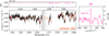 |
Fig. D.1 Same as Fig. 5 but for Luhman 16A. |
| In the text | |
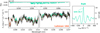 |
Fig. D.2 Same as Fig. 6 but for Luhman 16A. |
| In the text | |
Current usage metrics show cumulative count of Article Views (full-text article views including HTML views, PDF and ePub downloads, according to the available data) and Abstracts Views on Vision4Press platform.
Data correspond to usage on the plateform after 2015. The current usage metrics is available 48-96 hours after online publication and is updated daily on week days.
Initial download of the metrics may take a while.