| Issue |
A&A
Volume 656, December 2021
|
|
|---|---|---|
| Article Number | A97 | |
| Number of page(s) | 11 | |
| Section | Planets and planetary systems | |
| DOI | https://doi.org/10.1051/0004-6361/202141412 | |
| Published online | 08 December 2021 | |
The influence of gravity on granular impacts
I. A DEM code performance comparison
1
Institut Supérieur de l’Aéronautique et de l’Espace,
Av. Edouard Belin,
31400
Toulouse cedex 4,
France
e-mail: cecily.sunday@isae-supaero.fr
2
Université Côte d’Azur, Observatoire de la Côte d’Azur, CNRS, Laboratoire Lagrange, Bd de l’Observatoire,
CS 34229,
06304
Nice cedex 4,
France
3
Centre National d’Études Spatiales,
Av. Edouard Belin,
31400
Toulouse cedex 4,
France
Received:
28
May
2021
Accepted:
22
September
2021
Context. Impacts on small-body surfaces can occur naturally during cratering events or even strategically during carefully planned impact experiments, sampling maneuvers, and landing attempts. A proper interpretation of impact dynamics allows for a better understanding of the physical properties and the dynamical process of their regolith-covered surfaces and their general evolution.
Aims. This work aims to first validate low-velocity, low-gravity impact simulations against experimental results, and then to discuss the observed collision behaviors in terms of a popular phenomenological collision model and a commonly referenced scaling relationship.
Methods. We performed simulations using the soft-sphere discrete element method and two different codes, Chrono and pkdgrav. The simulations consist of a 10-cm-diameter spherical projectile impacting a bed of approximately 1-cm-diameter glass beads at collision velocities up to 1 m s−1. The impact simulations and experiments were conducted under terrestrial and low-gravity conditions, and the experimental results were used to calibrate the simulation parameters.
Results. Both Chrono and pkdgrav succeed in replicating the terrestrial gravity impact experiments with high and comparable computational performance, allowing us to simulate impacts in other gravity conditions with confidence. Low-gravity impact simulations with Chrono show that the penetration depth and collision duration both increase when the gravity level decreases. However, the presented collision model and scaling relationship fail to describe the projectile’s behavior over the full range of impact cases.
Conclusions. The impact simulations reveal that the penetration depth is a more reliable metric than the peak acceleration for assessing collision behavior in a coarse-grained material. This observation is important to consider when analyzing lander-regolith interactions using the accelerometer data from small-body missions. The objective of future work will be to determine the correct form and applicability of the cited collision models for different impact velocity and gravity regimes.
Key words: minor planets, asteroids: general / planets and satellites: surfaces / methods: numerical / methods: miscellaneous
© C. Sunday et al. 2021
 Open Access article, published by EDP Sciences, under the terms of the Creative Commons Attribution License (https://creativecommons.org/licenses/by/4.0), which permits unrestricted use, distribution, and reproduction in any medium, provided the original work is properly cited.
1 Introduction
After decades of study, scientists still struggle to describe the complex process that occurs when an object is dropped onto a bed of granular material. Impact dynamics have been investigated extensively using laboratory experiments in order to explain how collision behavior scales with factors such as the projectile size, impact velocity, and target surface material (Omidvar et al. 2014; Katsuragi 2016). A particular variable of interest, though one that is much more difficult to study, is gravity. Understanding the role that gravity plays in granular collisions is essential to optimize our gain from future planetary exploration missions. For example, accurate collision models can help us design systems to land and operate on asteroid surfaces, as well as improve our ability to deduce a body’s surface material properties from the size and shape of its craters. The response of planetary surfaces to impacts is also highly important for understanding the bodies’ geophysical evolution, and for providing accurate estimates of surface ages (Marchi et al. 2015).
Experimentally, slow impacts have been studied for low-gravity conditions using drop-tower setups (Goldman & Umbanhowar 2008; Altshuler et al. 2014; Murdoch et al. 2017, 2021; Brisset et al. 2020), parabolic flights (Brisset et al. 2018), space-shuttle missions (Colwell & Taylor 1999; Colwell 2003), and fluidized granular beds (Costantino et al. 2011; Brzinski et al. 2013). The physical limitations of these setups, however, coupled with their high cost and complexity, have made it difficult to construct a large database with established collision information. Thanks to increasing computational resources and the development of robust algorithms in the last decades, numerical modeling has emerged as a useful tool to help extend these low-gravity test campaigns. Numerical modeling has also been used to investigate other types of phenomena on small bodies, such as grain segregation, seismic shaking, and high-speed impacts (Tancredi et al. 2012; Matsumura et al. 2014; Sánchez & Scheeres 2021).
In this study, we use the soft-sphere discrete element method (SSDEM) to numerically model slow impacts on granular materials under Earth and low-gravity conditions. Our ultimate objective is to build upon the low-gravity impact analysis that was recently presented by Murdoch et al. (2021). The goals of this specific work are (1) to validate and calibrate the numerical simulations and (2) to compare one set of low-gravity simulations against the experimental results reported in Murdoch et al. (2021). Simulations with a larger range of target materials, impact velocities and gravity levels will be presented in a future study.
We begin by performing impact experiments into glass beads under terrestrial gravity. Then, we reproduce the experiments using two different SSDEM codes, and lastly, we use one of the codes to conduct impact simulations for a gravity level of 0.1 m s-2. The primary reason for using two SSDEM codes is to see if differences in the codes’ implementation or parallelization methods lead to noticeable differences in their results or computational performances. The comparison exercise also allows us to identify the appropriate simulation parameters for both codes and to validate both codes against the experimental data so that either can be used for future impact studies.
The remainder of this paper is organized as follows. In Sect. 2, we present the experimental and simulation setups, and we describe the two SSDEM codes, Chrono and pkdgrav, in more detail. In Sect. 3, we compare the outputs of the simulations against each other and against the experimental results. We identify the simulation parameters that generate the best match between the numerical and experimental results, and we compare the computational performances of the two codes. In Sect. 4, we conduct low-gravity impact simulations with Chrono, and we discuss the results in terms of an existing phenomenological collision model (Katsuragi & Durian 2007; Murdoch et al. 2021) and an established impact scaling relationship (Uehara et al. 2003; Ambroso et al. 2005). Finally, we summarize our findings and plans for future work in Sect. 5.
2 Method
2.1 Experimental setup
Impact experiments were conducted by dropping a 10 cm diameter, 1 kg spherical projectile from rest into a cylindrical container filled with 1 ± 0.3 cm glass beads. The container measures 31.5 cm in diameter at its base and 35 cm in diameter at its top rim. It was filled to a nominal height of 17 cm, and the beads were mixed and flattened before each trial to ensure repeatability. This preparation method results in a material bulk density of approximately 1.5 g cm−3. The initial drop height of the projectile was adjusted between 1 and 5 cm above the surface of the beads in order to generate impact velocities ranging from 0.4 to 1 m s−1. Finally, an accelerometer was mounted inside of the projectile in order to measure the projectile’s acceleration profile throughout each collision. For more information on the experimental setup, see Murdoch et al. (2021).
2.2 Numerical simulations
The impact experiments described in Sect. 2.1 were replicated numerically using two different SSDEM codes: Chrono and pkdgrav. The codes are presented in more detail in Sects. 2.2.1 and 2.2.2, but the shared setup procedure is outlined below.
In the simulations, the container is modeled using a 31.5 cm diameter cylindrical wall with a disk at the bottom, and it is filled with grains to a nominal height of 10 cm. The grains are 1 ± 0.05 cm in diameter and have a measured density of 2.48 g cm−3. In Chrono (Tasora et al. 2016), the impactor is modeled as a solid sphere while in pkdgrav (Richardson et al. 2000), it is modeled as a shell wall (Richardson et al. 2011). At the beginning of each simulation, the particles are mixed inside of the container and are permitted to settle until the average (root-mean squared, or RMS) speed of the grains falls below 1 × 10⁻³ cm s−1 and the maximum speed of any individual grain in the system falls below 0.1 cm s−1. Next, the surface is flattened by removing any particles above a specified fill height (e.g., 10 cm in the nominal case). Then, the projectile is dropped from a predefined height above the surface, and lastly, the simulation terminates when the projectile’s speed falls below 0.1 cm s−1. Figure 1 presents snapshots from the beginning and end of an example simulation.
Table 1 summarizes the baseline parameters for the Chrono and pkdgrav simulations. Though Chrono and pkdgrav both use the soft-sphere discrete element method, the two codes implement different contact force models, rolling friction models, twisting friction models and integrators. The normal and tangential contact forces in Chrono are determined using the nonlinear Hertz model, and the relevant equations and relationships can be found in Appendix A of Sunday et al. (2020). The normal and tangential contact forces in pkdgrav are calculated using the linear Hooke model, and the relevant equations and relationships can be found in Sects. 2.1–2.3 of Schwartz et al. (2012). The rolling and twisting friction models that are implemented in the Chrono code are described in Sect. 3.4 of Sunday et al. (2020), and the friction models that are used in pkdgrav are described in Sect. 2.2 of Zhang et al. (2017).
Since Chrono and pkdgrav use different force and resistance models, the codes require different input parameters. In some cases, the names of the input parameters appear to be the same, but the values are different because they are related to the specific models in each code. For example, pkdgrav uses an input value called the shape parameter to account for the contributionof a particle’s shape to the bulk friction of a material. The inter-particle friction is controlled by adjusting both the shape parameters and the friction coefficients. The friction models in Chrono do not include a shape parameter, so the user-specified values for the friction coefficients are notably different than those used by pkdgrav.
Another important difference between the codes is how they determine the stiffness and damping coefficients for the particle-particle and particle-wall contacts. Both codes include the option to directly specify the normal and tangential stiffness coefficients, but they also have built-in functions that can derive the values from other input parameters. In this study, we opted to use the built-in functions because these methods are frequently adopted by code users to determine the optimal coefficients for the contacts. In pkdgrav, the stiffness and damping coefficients are calculated using the normal and tangential coefficients of restitution, among other parameters (see Sects. 2.1–2.3 in Schwartz et al. 2012). In Chrono, the coefficients are determined from input valueslike the Young’s modulus, the Poisson’s ratio, and the normal coefficient of restitution (see Appendix A in Sunday et al. 2020). This is why Table 1 includes values like the Young’s modulus for Chrono, but not for pkdgrav, and the tangential coefficient of restitution for pkdgrav but not for Chrono. Sects. 2.2.1 and 2.2.2 provide general overviews of Chrono and pkdgrav and comment on the differences between the two codes in more detail. Then, Sect. 2.2.3 describes the specific parameters that were varied in order to compare the codes and conducttargeted studies.
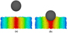 |
Fig. 1 Depiction of an example Chrono simulation when (a) the projectile is released from a height of 5 cm above the bed’s surface and (b) the projectile is considered to be at rest in the material. The container is 31.5 cm in diameter and is filled to a height of 12 cm. The projectile is 10 cm in diameter and 1 kg in mass. The spherical beads are 1 ± 0.05 cm in diameter and are colored by their radial position from the center of the container at the beginning of the simulation. |
Baseline SSDEM parameters for the Chrono and pkdgrav impact simulations.
2.2.1 Simulations with Chrono
Chrono is an open-source code that can be used to simulate rigid body interactions, soft body interactions, and even interactions between solids and fluids (Tasora et al. 2016). Among other capabilities, it includes modules for performing Finite Element Analysis (FEA) and for developing sensors for autonomous vehicle systems (Elmquist et al. 2021). This study makes use of the Chrono::Multicore module (in Chrono 5.0.0 and older, Chrono::Multicore is named Chrono::Parallel). Chrono::Multicore allows users to simulate granular systems with SSDEM (known as SMC, or the SMooth Contact model in Chrono) using shared-memory parallel computing with OpenMP. Contacts between particles are identified and evaluated according to a two-phase collision detection algorithm (Mazhar et al. 2013), and the system is advanced with a first-order Euler implicit linearized integrator.
The SSDEM code in Chrono::Multicore was recently modified to include rolling and twisting friction and to include additional force and cohesion models (Sunday et al. 2020). The rolling and twisting friction models are velocity dependent and were implemented to match the models found in early versions of pkdgrav (Schwartz et al. 2012). The modified Chono::Multicore code (available in Chrono 5.0.0 and newer) was validated though a series of simple two-body collision tests, piling simulations, and rotating drum tests (Sunday et al. 2020).
Table 1 summarizes the parameters that were used for the Chrono simulations in this study. Following the work of Schwartz et al. (2014), the normal coefficient of restitution (COR) for the walls is set to 0.5 while the normal COR for the grains is set to 0.9. Experiments have shown that rocky materials have a COR of 0.8–0.9 for impact velocities ranging from 1 to 2 m s−1 (Imre et al. 2008; Durda et al. 2011). Tancredi et al. (2012) observe COR values in this range by simulating collisions between two spheres using the Hertz contact model and a particle material with a higher Young’s modulus and Poisson’s ratio than used here (E = 1 × 10¹⁰ Pa and ν = 0.3). Schwartz et al. (2014) find that simulations with higher COR values provide a good match for low-speed impact experiments into glass beads, so a normal COR value of 0.9 was used for this study. With the exception of the coefficient of restitution and the grain density, the remaining glass bead material properties were selected based on the work of Sunday et al. (2020). The method for determining the simulation time step is discussed in Sect. 3.2.
2.2.2 Simulations with pkdgrav
Pkdgrav is an N-body gravity tree-code (Richardson et al. 2000, 2009, 2011; Stadel 2001) that models interactions between grains according to the SSDEM implementation by Schwartz et al. (2012). The code was later improved by Zhang et al. (2017) with a new rotational resistance model for twisting and rolling friction, by Zhang et al. (2018) with a cohesion force model for characterizing van der Waals cohesive forces between interstitial fine grains, and by Maurel et al. (2018) with the introduction of “reactive walls”, namely inertial walls that can react to the forces exerted by the grains (in contrast to traditional walls in pkdgrav whose motion is predefined and is not affected by contacts with grains).
Advantages of pkdgrav include full support for parallel computation (supporting both shared-memory parallel computing with Pthreads and distributed-memory parallel computing with MPI), the use of hierarchical tree methods to rapidly compute long-range inter-particle forces (e.g., gravity) and to locate nearest neighbors for computing short-range contact forces and potential colliders, and options for particle bonding to make irregular rigid aggregates. Pkdgrav uses a second-order leapfrog integrator: in each step, particle positions and velocities are alternately “drifted” and “kicked” (see Richardson et al. 2009, for details). Collision searches are performed during the drift step by examining the trajectories of neighbors for each particle to ensure no collisions are missed. A hierarchical tree data structure is used to detect collisions between particles at each time step and generate particle neighbor lists in  time, where N is the number of particles in the simulation (Richardson et al. 2011). The code has been validated through comparisons with experiments and other numerical codes for diverse applications, such as hopper discharges (Schwartz et al. 2012), low-speed impacts (Schwartz et al. 2014; Ballouz 2017; Thuillet et al. 2020), sandpiles and avalanches (Yu et al. 2014), angle-of-repose experiments (Maurel et al. 2018), and triaxial compression tests (Zhang et al. 2018).
In pkdgrav, contacts between grains are ruled by several physical parameters, such as the three friction coefficients (i.e., sliding μs, rolling μr, and twisting μt), the shape parameter β, and the normal and tangential coefficients of restitution en and et. The shape parameter β represents the angularity of grains and plays a role in the rolling and twisting friction, as well as in the angle of repose of the material. These parameters are more thoroughly described in Schwartz et al. (2012), Zhang et al. (2017, 2018), and Maurel et al. (2018).
Table 1 lists the parameters for the pkdgrav simulations that were performed in this study. The normal COR value for the grains was set to 0.9 for the reasons discussed in Sect. 2.2.1, and the tangential COR value for the grains was set to 1.0 based on experimental measurements by Yu et al. (2014). The same tangential COR value was applied by Ballouz (2017) to model glass beads in another study and is used here for both the grains and walls. For details on how the simulation time step is calculated, refer to Schwartz et al. (2012).
2.2.3 Investigated parameters
To obtain a comprehensive understanding of the effect of different simulation parameters, we conduct five groups of investigations. The fill height of the container is varied to find the minimum bed height for which the boundary conditions no longer influence collision behavior (Sect. 3.1). In Chrono, the time step is varied to confirm that the appropriate step value was selected for the study (Sect. 3.2). In order to find the simulation parameters that generate a best match between numerical and experimental results, the coefficients of rolling and twisting friction are varied in Chrono, and the coefficient of rolling friction and the shape parameter are varied in pkdgrav (Sect. 3.3). The results from the friction analysis are then used to compare the computation performance of the two codes (Sect. 3.4). Finally, Chrono is used to compare impact behavior for two different gravity levels, and the observations are discussed alongside findings from Murdoch et al. (2021) and Ambroso et al. (2005) (Sect. 4).
2.3 Data analysis
Collision behavior is often characterized using three values: the peak acceleration of the projectile, the maximum penetration depth of the projectile, and the total duration of the collision. During the experimental trials, the projectile’s acceleration was logged at a sampling frequency of 1.4 kHz using an accelerometer mounted to the inside of the projectile. The projectile’s velocity and position profiles were then obtained by integrating the acceleration data. The beginning of the collision is identified as the moment when the projectile is no longer in free-fall, and the end of the collision is defined as the moment when the projectile’s acceleration falls below a threshold value of 0.1g. For more information on the accelerometer specifications or the processing of the experimental data, please refer to Murdoch et al. (2021).
Chrono and pkdgrav report the acceleration, the velocity, and the position of the projectile as direct simulation outputs. The data from the Chrono and pkdgrav simulations were sampled at a frequency of 10 kHz and 100 kHz respectively, which is much higher than the sampling frequency of the experimental data. To make the data sets more comparable, the experimental and simulation data was filtered using a second order Butterworth filter with a cut-off frequency of 500 Hz. The cut-off frequency was chosen to beslightly lower than the Nyquist frequency of the lowest sampling rate (i.e., the sampling rate of the experimental data). The collision durations for the Chrono and pkdgrav simulations were then found using the same method as described above for the experimental data.
Figure 2 shows the acceleration, the velocity, and the position profiles for a typical experiment (shown in black), a Chrono simulation (shown in blue), and a pkdgrav simulation (shown in red). In this example, the projectile impacts the bed at approximately 1 m s−1. Annotations are used to indicate the collision velocity vc, the peak acceleration apeak, the penetration depth zstop, and the collision duration tstop. To check forconsistency between the simulation data and the method for processing the experimental data, we also determine the projectile’s velocity and position by integrating the acceleration data from the Chrono simulation. The results of the alternative processing method, shown in green, match the raw simulation data and the processed experimental data well.
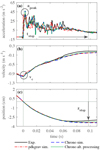 |
Fig. 2 Acceleration, velocity, and position profiles for an example experiment (black), a Chrono simulation (blue), and a pkdgrav simulation (red). The green line shows the Chrono simulation data when processed using the same method as the experimental data. The projectile’s approximate collision velocity vc, peak acceleration apeak, penetration depth zstop, and collision duration tstop are indicated by the black text and arrows. |
3 Results
3.1 Container fill height
An experimental study by Nelson et al. (2008) concludes that a finite container size will not influence collision behavior as long as impact velocities are low, the container diameter is at least three projectile diameters in width, and the container fill height is approximately one projectile diameter in depth. Containers with undersized radii have been shown to generate artificially low penetration depths (Nelson et al. 2008; Seguin et al. 2008; Goldman & Umbanhowar 2008). In contrast, containers with shallow fill heights seem to have little influence on penetration depth, as long as the projectile does not rebound off of the bottom of the container (Nelson et al. 2008; Seguin et al. 2008).
In this work, the container diameter is considered fixed and is equal to 3.15 times the diameter of the projectile. In order to find the fill height where the collision behavior becomes constant and where the behavior is independent of the bed depth, we conducted experiments and simulations with fill heights ranging from 2 to 14 cm. Figure 3 shows the measured penetration depth for 1 m s−1 collisions as a function of the container fill height for a series of experiments (shown in black), Chrono simulations (shown in blue), and pkdgrav simulations (shown in red). The error bars on the data points for the experiments and the Chrono simulations represent the standard deviation of at least three test repetitions, while the shaded region on the plot indicates fill height where rebounds were observed. The parameters that were used for the simulations are the same as those listed in Table 1, with the exception of the shape parameter in pkdgrav which was set to 0.1. In both the experiments and the simulations, the projectile rebounds off of the bottom of the container when the fill height is less than or equal to 4 cm. The projectile’s penetration depth appears to be more or less constant when the fill height is greater than or equal to 6 cm. Based on these findings, and the work by Nelson et al. (2008), all remaining simulations were executed with a conservative fill height of 10 cm.
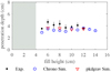 |
Fig. 3 Final penetration depth for impacts at 1 m s−1 for differentcontainer fill heights. The error bars for the experiments and the Chrono simulations are based on the standard deviation of at least three test repetitions, and the gray shaded region indicates the fill heights where the projectile rebounded after hitting the bottom surface of the container. |
3.2 Time step
The time step for SSDEM simulations should be selected such that the step size is much smaller than the duration of any given collision in the system. The typical duration of a collision τ is calculated according Hertzian contact theory for the Chrono simulations and Hookean contact theory for the pkdgrav simulations. In Hertzian contact theory, parameters like the particle density, the particle radius, the Poisson’s ratio and the Young’s modulus influence the collision duration. In Hookean theory, the collision duration depends on the mass, the stiffness, and the damping properties of the material. The full expressions for τ based on Hertzian and Hookean theory can be found in Tancredi et al. (2012) and Schwartz et al. (2012) respectively.
It is common to select a time step Δt that is 10 to 50 times smaller than τ. However, the integrator type and the specific implementations of rolling and twisting friction in Chrono can lead to numerical instability when the system is in a quasi-static state and the time step is either too large or excessively small. To verify that the proper time step was selected for this study, we varied the time step in Chrono between 10 μs (approximately 1/10 τ) and 0.5 μs (approximately 1/300 τ). Figure 4 shows the projectile’s collision behavior for the different time steps. There is no observable difference in the penetration depth or the collision duration for the selected range of values, but there is a slight increase in the peak acceleration for the smallest time step and the highest collision velocities. A potential explanation for this difference is given in Sect. 5. Based on the results shown in Fig. 4, a conservative but reasonable time step value of 1 μs was selectedfor the remaining Chrono simulations.
3.3 Friction
Most of the material properties for the simulated glass beads were selected to either match the characteristics of the actual beads or to match values from previous numerical studies (see Sects. 2.2.1 and 2.2.2). Here, we adjust the frictional properties of the beads to find the values that generate a reasonable fit between the experimental and numerical results.
In Chrono, the coefficient of rolling friction μr was varied between 0 and 0.25 while the coefficient of twisting friction μt was set to zero. Then, μt was varied between 0 and 0.1 while μr was set to 0.09. Figure 5 shows how the projectile’s collision behavior changes for select values of μr when μt = 0. Several different rolling friction coefficients succeed in reproducing the experimental results because μr has a diminishing effect on collision behavior as μr increases. The same phenomenon was observed in Sunday et al. (2020) during angle of repose simulations. Figure 6 illustrates the relationship between penetration depth and μr more clearly. The data points in Fig. 6 correspond to impact simulations where vc = 1.02 ± 0.03 m s−1 and μt = 0. As μr increases from 0 to about 0.13, the penetration depth decreases. As μr increases from 0.13 to 0.25, the penetration depth remains more or less the same. The simulation results from Chrono best match the experimental results when μr ≥ 0.09.
Unlike the coefficient of rolling friction, varying the coefficient of twisting friction μt does not have an observable effect on the sphere’s collision behavior, at least for impact simulations where μt = 0–0.1 and μr = 0.09. A nonzero baseline value of μt = 0.01 was selected for the remaining Chrono simulations in order to allow for a performance comparison with the pkdgrav simulations, which also use a nonzero μt value.
The relationship between a material’s angles of repose and the friction parameters in pkdgrav has been characterized by previous studies. Different combinations of pkdgrav parameters can generate the same angle of repose, so to decrease the degrees of unknowns, the coefficients of sliding and twisting friction were set to 1.0 and 1.3 respectively. These values have been extensively calibrated with triaxial compression experiments by Zhang et al. (2018) and were previously used by Maurel et al. (2018) and Thuillet et al. (2018). Here, simulations were conducted using these values and different combinations of the shape parameter β and the coefficient of rolling friction μr. β was varied between 0.0025 and 0.3 and μr was varied between 0.5 and 2.0. The angles of repose measurements that correspond to these parameter combinations are shown in Table 2.
Figure 7 shows the projectile’s collision behavior for a subset of the parameter combinations in pkdgrav. When comparing Figs. 5 and 7, it appears as though the results for the Chrono simulations have a higher scatter than the results for the pkdgrav simulations. The difference is possibly related to a slight variation in the test setup between the two codes. In Chrono, three tests were repeated for seven different impact velocities. At the start of each test, the sphere’s radial and vertical position was randomly varied within two grain diameters to add variability to the initial impact configuration. By contrast, one pkdgrav simulation was conducted for 11 different collision velocities. The starting height of the projectile was varied between each test, but not its radial position. Regardless of the scatter, the results for the two codes show similar trends. As in the Chrono simulations, increasing the coefficient of rolling friction in pkdgrav results in a decrease of the penetration depth and the collision duration. Increasing the shape parameter, which is like increasing the angularity of the particles, also causes in a decrease of the penetration depth and the collision duration. The simulation results from pkdgrav best match the experimental results when μr = 0.5 and β = 0.1 and when μr = 1.05 and β = 0.05. These parameter combinations correspond to angles of repose of 23.2 and 22.1 degrees respectively, which are comparable to the typical repose angle for glass beads (see Table 2). Thoughnot shown in Fig. 7, the simulations also match the experiments when μr = 1.05 and β = 0.075. This combination of parameters corresponds to an angle of repose of 23.5 degrees and gives almost identical results as when μr = 0.5 and β = 0.1.
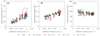 |
Fig. 4 Peak acceleration, penetration depth, and collision duration for simulations in Chrono with different time steps Δt. The penetration depth and collision duration remain constant within the selected range of time steps. |
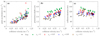 |
Fig. 5 Peak acceleration, penetration depth, and collision duration for simulations in Chrono with different coefficients of rolling friction μr. The coefficient of twisting friction μt = 0. The simulation results match the experimental data best when μr ≥ 0.09. |
Angle of repose measurements in pkdgrav for different combinations of μr and β when μs = 1.0 and μt = 1.3.
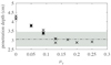 |
Fig. 6 Penetration depth by coefficient of rolling friction μr for simulations in Chrono where the collision velocity vc = 1.02 ± 0.03 m s−1 and the coefficient of twisting friction μt = 0. The dashed line shows the average penetration depth for the impact experiments in the same collision velocity range, and the shaded region gives the standard deviation from the mean. |
3.4 Code performance
The calibration tests described in Sect. 3.3 provide an opportunity to compare the overall performances of Chrono and pkdgrav. As previously discussed, the two codes implement different force and resistance models, and thus require different input parameters to accurately model the glass bead material. Despite their implementation and parameter differences, both codes successfully reproduce the collision behaviors observed in the experiments. In this section, we focus on the computational aspects of the two codes.
Chrono::Multicore is parallelized using the OpenMP application program interface (API) for shared-memory multiprocessing. We ran the Chrono simulations on an Intel® Xeon® Gold 6140 processor using 36 threads. Benchmark testing with this specific system has shown that the code’s performance is optimal when the simulations are executed on 24 threads, but that there islittle variation in the performance when the simulations are executed on 24–36 threads. The benchmark testing was performed for systems containing a few thousand to several hundred thousand particles, and the above two trends were found to be independent of the number of particles in the system.
When the container is filled to a height of 10 cm, the Chrono simulations contain 7940 particles. On average, the simulations require 2.5 μs per simulation step per particle to complete when executed on 36 threads. This means that a 0.5 s simulation with a 1 μs time step will finish in approximately 2.75 h. Closer profiling of the code reveals that over 60% of the total computation time is spent detecting and characterizing collisions (i.e., identifying which particles are in contact and extracting precise contact information like location and degree of overlap). About 35% of the computation time is spent calculating and resolving contact forces, and the remaining 5% of the time is spent updating the state information for each body (i.e., the particle position, velocity, and rotation vectors). The simulation run-time can be improved slightly, but not drastically, by tuning the input parameters associated with the collision detection algorithms (Mazhar et al. 2013). These algorithms are also more suited for dynamicsystems than for quasi-static systems, so simulations with large particle flow (e.g., the mixing of a material) will execute faster than simulations where the majority of the particles remain untouched in a particle bed.
In Chrono, the computation time increases linearly with the number of particles in the system. Figure 8 shows the total execution time for a 0.25 s benchmark test with a 10 μs time step and a system size ranging from about seven thousand to ten million particles. The benchmark test resembles the initial setup phase of the impact simulations (i.e., the mixing and settling of the material in the container). The trend implies that an impact simulation with one million particles will take 2.5 μs per step per particle to complete, just like the smaller system that was used for this study. However, a 0.5 s simulation with one millions particles and a 1 μs time step will take approximately 14.7 days to execute. Therefore, Using the Chrono::Multicore code to simulate very large granular systems is only feasible if the run-time of the simulation is short or if the simulation time step is relatively large.
pkdgrav supports both shared-memory parallel computing with Pthreads and distributed-memory parallel computing with MPI. In this study, we ran the pkdgrav simulations using the MPI implementation on dual Intel® Xeon® IvyBridge E5-2670v2 processors running at 2.50 GHz with FDR infiniband interconnects between nodes (each node contains 2 sockets with 10 cores per socket, that is, 20 cores in total; each socket is announced at 200 GFlops). This option allows us to test the effect of numbers of cores that are distributed on different nodes of the cluster.
For a direct comparison, we used the same fill height of 10 cm for the pkdgrav performance test, which contains 7987 particles. On average, the simulations require 3.6 μs per simulation step per particle to complete when the simulations are executed on 2 cores on one node, and this value decreases to 2.9 μs with 4 cores, to 2.5 μs with 8 cores, and converges to 2.3 μs with 16–20 cores. A 0.5 s impact simulation in pkdgrav with a 0.5 μs time step takes approximately 5.1 h to complete when executed on 20 cores on one node.
When the simulations are executed on two nodes, the performance decreases with the number of cores, that is, the computation time per step per particle increases to 2.8 μs with 25 cores, to 3.3 μs with 30 cores, and to 4.4 μs with 40 cores. This indicates that the time consumption on domain decomposition and communications between nodes dominate the parallel performance. For example, when running with 20 cores on one node, 10% of the computation time is spent decomposing the particle domain, and this ratio increases to 20% when running with 40 cores on two nodes. Nevertheless, the MPI module of pkdgrav can take advantage of the available nodes on the entire cluster and allow for modeling large-scale particle systems (e.g., in our previous study of modeling a granular system containing 1.6 million monodisperse particles, the computation time per step per particle is ~ 0.4 μs when running the code on 320 cores on 16 nodes; Zhang et al. 2021). A good rule of thumb based on past and current tests is to allocate ~ 1000 particles on each core to achieve the optimal performance. Due to the code’s ability to execute a simulation across multiple nodes, pkdgrav is much more suited for studying extremely large granular systems than Chrono::Multicore.
4 Discussion
Murdoch et al. (2021) conducted low-velocity impact experiments under terrestrial gravity and reduced-gravity levels for different projectile shapes and surface materials. The low-gravity tests were performed using an Atwood machine drop-tower (Sunday et al. 2016), with impact velocities ranging between 0.01 and 0.4 m s−1 and gravity levels ranging from 0.4 to 1.4 m s−2. The authors discuss their results in terms of the phenomenological impact model given by
 (1)
(1)
which was first proposed by Poncelet and was later investigated in depth by Katsuragi & Durian (2007), Tsimring & Volfson (2005), and others.
In Eq. (1), F is the total force acting on the projectile, m is the projectile mass, v is the projectile velocity, f(z) is the quasi-static resistance force, and h(z) is the inertial or the hydrodynamic drag force. If f(z) = f0 and h(z) = m∕d1, then exact solutions for the peak acceleration, the penetration depth, and the collision duration can be derived from Eq. (1) (refer to Murdoch et al. 2021, for details). The f0 and d1 terms are assumed to be constant and are determined by fitting the experimental data to Eq. (2), that is, the expression for the peak acceleration,
 (2)
(2)
Per Murdoch et al. (2021), the fit parameters f0 and d1 can be used to predict the final penetration depth of the projectile,
![\begin{equation*}z_{\mathrm{stop}}\,{=}\,\frac{d_{1}}{2}\ln \left[1+\frac{mv_{c}^{2}}{d_{1}(f_{0}-mg)} \right], \end{equation*}](/articles/aa/full_html/2021/12/aa41412-21/aa41412-21-eq4.png) (3)
(3)
and the total duration of the collision,
![\begin{equation*}t_{\mathrm{stop}}\,{=}\, \mathrm{atan} \left[v_{\textrm{c}} \sqrt{\frac{m}{d_1 (f_0 - mg)}}\ \right] \left[\frac{1}{d_1} \left(\frac{f_0}{m} -g \right)\ \right]^{-1/2}. \end{equation*}](/articles/aa/full_html/2021/12/aa41412-21/aa41412-21-eq5.png) (4)
(4)
With the help of numerical modeling, we can extend the range of test cases explored in Murdoch et al. (2021), where experimental results are presented for impacts into 1.5 mm glass beads with impact velocities ranging from 0.01 to 0.2 m s−1 and a minimum gravity level of 1.15–1.21 m s−2. Here, we use Chrono to simulate impacts into 10 mm glass beads with impact velocities ranging from 0.01 to 1.2 m s−1 and a gravity level of 0.1 m s−2. To avoid rebound, the container fill height for the low-gravity simulations was increased to 21 cm. Figure 9 shows the peak acceleration, the penetration depth, and the collision duration for both the terrestrial gravity tests and the low-gravity simulations. The lines on Fig. 9 a represent the model fit according to Eq. (2). The values of f0 and 1∕d1 that were determined from the fits shown in Fig. 9 a are listed in Table 3. The lines on Figs. 9 b and 9 c represent the predictions for the penetration depth and the collision duration based on the f0 and 1∕d1 fit values and Eqs. (3) and (4).
For all collision velocities, the penetration depth and the collision duration increase with decreased gravity. For the higher collision velocities, the collision duration is constant. These trends are consistent with observations from Murdoch et al. (2021). The model and the fit method from Murdoch et al. (2021) under-predicts the penetration depth for both the 1g and the low-gravity cases as well as the collision duration for the 1g case. At the same time, the model over-predicts the collision duration for the low-gravity case. Murdoch et al. (2021) did not observe such pronounced differences between the model predictions and the experimental data for the 1.5 mm glass bead experiments, but the authors did observe a distinct under-prediction for terrestrial gravity experiments with 5 mm glass beads. Theyindicate that the shortcoming of the method might be related to the coarse size of the simulated grains.
The conclusions from Murdoch et al. (2021) are in agreement with the popular notion that low-velocity impacts transition through tworegimes, a quasi-static regime and an inertial regime. They suggest that the regime transition occurs at the transition velocity vt given by
 (5)
(5)
Equation (5) can be derived from Eq. (1) by identifying the velocity where the quasi-static friction and the inertial drag forces are equal (Murdoch et al. 2021). The authors then go on to show that the transition velocity decreases as gravity decreases. Based on Eq. (5) and the fit parameters in Table 3, the simulations have a transition velocity of approximately 0.7 m s−1 for impacts under terrestrial gravity and a transition velocity of approximately 0.07 m s−1 for impacts in low-gravity, supporting the hypothesis from Murdoch et al. (2021). Table 3 provides the calculated transition velocities vt for all of the numerical and experimental results discussed in this section. In general, collisions that are dominated by inertial drag forces, that is, collisions where vc > vt, result in higher penetration depths than collisions that are dominated by quasi-static friction forces. Since the transition between the quasi-static and the inertial regime is continuous however, there is not a directly observable difference in the peak acceleration, the penetration depth, or collision duration measurements right at the transition velocity vt. The precise influence that the regime change has on factors like penetration depth and mobilized material will be discussed as part of future work.
Setting the Poncelet model (i.e., Eq. (1)) aside, penetration depth has also been shown to scale by the empirical relationship
 (6)
(6)
where D is the diameter of the projectile, ρp is the density of the projectile, ρg is the bulk density of the granular material, tan-1μ is the angle of repose of thegranular material, and H is the projectile’s drop height plus its final penetration depth (Uehara et al. 2003; Ambroso et al. 2005). This relationship was developed using the results from Earth-gravity impact experiments.
The specific form of this scaling relationship has been challenged by a number of experimental studies (de Bruyn & Walsh 2004; Tsimring & Volfson 2005; Goldman & Umbanhowar 2008; Brisset et al. 2020), but in general, the penetration depth zstop is proportional to Hα. The α value is most commonly expressed as a 1/3 power, but Tsimring & Volfson (2005) found that α = 2∕5, Seguin et al. (2009) reported that α = 0.31, and de Bruyn & Walsh (2004) found that α varies with the material packing fraction, where the value decreases from about 0.60 to 0.35 as the packing fraction increases from about 0.55 to 0.62.
Figures 10a and b show the relationship between the penetration depth zstop and the total height H for the 10 mm glass bead experiments and simulations. The α values for the Hα scaling law discussed above were determined by performing a linear regression with the data on a log-log scale. The blue lines in Fig. 10a show the resulting fits for the Chrono simulations, while the α values for all of the data sets are provided in Table 3. For comparison, Fig. 10b shows thedata with respect to the theoretical penetration depth that is calculated using the Poncelet model. The blue lines in Fig. 10b were generated using Eq. (3) and the f0 and d1 fit parameters for the Chrono simulations that are listed in Table 3.
Interestingly, in Fig. 10a, we observe a distinct difference in α for the terrestrial gravity and low-gravity test cases. The α value for the terrestrial gravity simulations is close to the 2/5 power scaling reported by Tsimring & Volfson (2005). The value for the low-gravity simulations tends toward a 2/5 scaling at low H values, but actuallyapproaches the 1/3 power scaling reported by Uehara et al. (2003) and Ambroso et al. (2005) for higher H values. The intercept for the two gravity levels is also different, which suggests that the constant in the empirical scaling relation (i.e., Eq. (6)) should also vary with gravity. The difference in the scaling values might simply be a consequenceof the relatively small number of data points in the study. An alternative possibility is that the scaling is dependent on the regime that dominates the collision behavior. According to the transition velocities shown in Table 3, the majority of the tests under terrestrial gravity are dominated by the quasi-static regime while the majority of the tests in low-gravity simulations are dominated by the inertial regime. Figure 10b supports this hypothesis. If the penetration depth follows the Poncelet model, then the height relationship is not linear on a log–log scale. We can also see that the curves for the different gravity levels are similar, but that they run more or less parallel to one another. This phenomenon will be investigated further as part of future work.
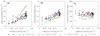 |
Fig. 7 Peak acceleration, penetration depth, and collision duration for simulations in pkdgrav with different coefficients of rolling friction μr and shape parameters β. The coefficient of static friction μs = 1.0 and the coefficient of twisting friction μt = 1.3. The simulation results match the experimental data best when μr = 0.5 and β = 0.1 and when μr = 1.05 and β = 0.05. |
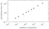 |
Fig. 8 Execution time by number of particles for a 0.25 s benchmark test in Chrono with a 10 μs time step. The test resembles the setup phase of the impact simulations (i.e., the mixing and initial settling of the material). With the exception of the time step, the simulation parameters match the values provided in Table 1. |
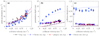 |
Fig. 9 Peak acceleration, penetration depth, and collision duration for the experiments, the Chrono simulation, and the pkdgrav simulations with a gravity of 9.81 m s−2 and the Chrono simulations with a gravity of 0.1 m s−2. The lines represent the model fits and model predictions that were determined according to Murdoch et al. (2021). |
Fit parameters for the 10 mm glass bead impact experiments and simulations from this work and the 1.5 mm glass bead experiments from Murdoch et al. (2021).
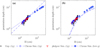 |
Fig. 10 Penetration depth zstop by total height H for the 10 mm glass bead experiments and simulations. H is the drop height plus the penetration depth. The blue lines in plot (a) represent the data fits to zstop ~ Hα for the Chrono simulations. The α values for all of the data sets are listed in Table 3. The blue lines in plot (b) represent the penetration depth relationship for the Chrono simulations based on Eq. (3) (i.e., the Poncelet model) and the fit parameters provided in Table 3. |
5 Conclusions
Understanding the role that gravity plays in granular collisions is essential for future planetary exploration involving surface interactions,for understanding the physical properties and geophysical evolution of small bodies, and for providing accurate estimates of their surface ages. We simulated low-velocity impacts on granular materials using SSDEM and two different codes, Chrono and pkdgrav. After calibrating the simulation friction parameters, the simulation results correspond well with the measurements from experimental trials. By varying the fill height of the material inside of the container, we find that a projectile’s collision behavior is independent of the fill height as long as the projectile does not rebound off of the bottom of the container. When the simulation time step is varied in Chrono, the projectile’s collision behavior remains unchanged within the selected range of time step values. Even though Chrono and pkdgrav implement different force models, friction models, and integrators, both codes successfully replicate the impact experiments when they use the appropriate simulation parameters. The computational performance of Chrono and pkdgrav is also comparable, despite differences in their contact-detection algorithms and their parallelization methods. At the same time, pkdgrav is better suited for large simulations (i.e., systems containing more than a few hundred thousand particles).
In every test set, we observe a much larger scatter in the projectile’s peak acceleration measurement than its penetration depth measurement. This scatter is likely related to the discrete nature of the surface material and the large size of the grains. The peak acceleration is sensitive to the specific arrangement of the surface beads underneath the falling projectile, while the penetration depth is not. The peak acceleration is also dependent on the capabilities of the sensor and the filtering method that is used to process the data. The penetration depth might be difficult to interpret for nonhomogeneous or slopped terrains, but for relatively flat surfaces, it provides a more repeatable measurement than the peak acceleration. This suggests that for certain applications, the penetration depth should be the primary term that is used to characterize collision behavior, not the peak acceleration. The reliability of the different collision parameters will be investigated in more detail in future work.
Impact simulations for terrestrial (g = 9.81 m s−2) and low (g = 0.1 m s−2) gravity levels show that the penetration depth and the collision duration both increase when the gravity level decreases. Murdoch et al. (2021) made the same observation, but for a higher gravity level and a smaller range of impact velocities. The generalized Poncelet model given by Eq. (1) fails to accurately describe the projectile’s collision behavior when the model fit parameters are determined using the peak acceleration measurement. The commonly referenced zstop ∝ H1∕3 scaling law also fails to describe the penetration depth for the full set of experimental and numerical results. It is possible that these commonly used collision models are applicable only for specific ranges of impact velocities. As part of future work, the suitability of these models will be investigated in much more detail. Simulations will be conducted using either Chrono or pkdgrav for a wider range of impact velocities and gravity levels, and the behavior predictions based on the Poncelet model will be revised to account for alternative assumptions, such as a depth-dependent quasi-static friction term (Tsimring & Volfson 2005; Brzinski et al. 2013) or the inclusion of a viscous drag term (de Bruyn & Walsh 2004). The goal of future work will be to scale the projectile’s collision behavior based on gravity and to identify the forms of the Poncelet model that best describe different impact regimes.
Acknowledgements
C.S. is funded jointly funded by the Centre National d’Études Spatiales (CNES) and the Institut Supérieur de l’Aéronautique et de l’Espace (ISAE) under a PhD research grant, and F.T. was supported through a PhD fellowship from the University of Nice-Sophia. All authors acknowledge support from CNES, and F.T and P.M. acknowledge funding from Academies of Excellence: Complex systems and Space, environment, risk, and resilience, part of the IDEX JEDI of the Université Côte d’Azur. P.M. and Y.Z. acknowledge funding from the European Union’s Horizon 2020 research and innovation program under grant agreement No. 870377 (project NEO-MAPP). Y.Z. acknowledges funding from the Doeblin Federation and the “Individual grants for young researchers” program, part of the IDEX JEDI of the Université Côte d’Azur. Simulations with Chrono were performed using HPC resources from CALMIP under grant allocation 2019-P19030 and simulations with pkdgrav were performed at Mésocentre SIGAMM hosted at the Observatoire de la Côte d’Azur.
References
- Altshuler, E., Torres, H., González-Pita, A., et al. 2014, Geophys. Res. Lett., 41, 3032 [NASA ADS] [CrossRef] [Google Scholar]
- Ambroso, M., Santore, C., Abate, A., & Durian, D. J. 2005, Phys. Rev. E, 71, 051305 [NASA ADS] [CrossRef] [Google Scholar]
- Ballouz, R.-L. 2017, PhD thesis, University of Maryland, College Park, USA [Google Scholar]
- Brisset, J., Colwell, J., Dove, A., et al. 2018, Progr. Earth Planet. Sci., 5, 1 [NASA ADS] [CrossRef] [Google Scholar]
- Brisset, J., Cox, C., Anderson, S., et al. 2020, A&A, 642, A198 [NASA ADS] [CrossRef] [EDP Sciences] [Google Scholar]
- Brzinski, III, T. A., Mayor, P., & Durian, D. J. 2013, Phys. Rev. Lett., 111, 168002 [CrossRef] [Google Scholar]
- Colwell, J. E. 2003, Icarus, 164, 188 [Google Scholar]
- Colwell, J. E., & Taylor, M. 1999, Icarus, 138, 241 [NASA ADS] [CrossRef] [Google Scholar]
- Costantino, D., Bartell, J., Scheidler, K., & Schiffer, P. 2011, Phys. Rev. E, 83, 011305 [NASA ADS] [CrossRef] [Google Scholar]
- de Bruyn, J. R., & Walsh, A. M. 2004, Can. J. Phys., 82, 439 [NASA ADS] [CrossRef] [Google Scholar]
- Durda, D. D., Movshovitz, N., Richardson, D. C., et al. 2011, Icarus, 211, 849 [CrossRef] [Google Scholar]
- Elmquist, A., Serban, R., & Negrut, D. 2021, J. Autonomous Veh. Syst., 1, 021001 [Google Scholar]
- Goldman, D. I., & Umbanhowar, P. 2008, Phys. Rev. E, 77, 021308 [NASA ADS] [CrossRef] [Google Scholar]
- Imre, B., Räbsamen, S., & Springman, S. M. 2008, Comput. Geosci., 34, 339 [NASA ADS] [CrossRef] [Google Scholar]
- Katsuragi, H. 2016, Physics of Soft Impact and Cratering, 1st edn., Lecture Notes in Physics 910 (Springer Japan) [CrossRef] [Google Scholar]
- Katsuragi, H., & Durian, D. J. 2007, Nat. Phys., 3, 420 [Google Scholar]
- Marchi, S., Chapman, C. R., Barnouin, O. S., Richardson, J. E., & Vincent, J.-B. 2015, Asteroids IV, 725 [Google Scholar]
- Matsumura, S., Richardson, D. C., Michel, P., Schwartz, S. R., & Ballouz, R.-L. 2014, MNRAS, 443, 3368 [NASA ADS] [CrossRef] [Google Scholar]
- Maurel, C., Michel, P., Biele, J., Ballouz, R.-L., & Thuillet, F. 2018, Adv. Space Res., 62, 2099 [Google Scholar]
- Mazhar, H., Heyn, T., Pazouki, A., et al. 2013, Mech. Sci., 4, 49 [NASA ADS] [CrossRef] [Google Scholar]
- Murdoch, N., Avila Martinez, I., Sunday, C., et al. 2017, MNRAS, 468, 1259 [NASA ADS] [Google Scholar]
- Murdoch, N., Drilleau, M., Sunday, C., et al. 2021, MNRAS, 503, 3460 [NASA ADS] [CrossRef] [Google Scholar]
- Nelson, E., Katsuragi, H., Mayor, P., & Durian, D. J. 2008, Phys. Rev. Lett., 101, 068001 [NASA ADS] [CrossRef] [Google Scholar]
- Omidvar, M., Iskander, M., & Bless, S. 2014, Int. J. Impact Eng., 66, 60 [Google Scholar]
- Richardson, D. C., Quinn, T., Stadel, J., & Lake, G. 2000, Icarus, 143, 45 [Google Scholar]
- Richardson, D. C., Michel, P., Walsh, K. J., & Flynn, K. W. 2009, Planet. Space Sci., 57, 183 [Google Scholar]
- Richardson, D. C., Walsh, K. J., Murdoch, N., & Michel, P. 2011, Icarus, 212, 427 [Google Scholar]
- Sánchez, P., & Scheeres, D. J. 2021, in EPJ Web of Conferences, 249, (EDP Sciences), 13001 [CrossRef] [EDP Sciences] [Google Scholar]
- Schwartz, S. R., Richardson, D. C., & Michel, P. 2012, Granular Matter, 14, 363 [Google Scholar]
- Schwartz, S. R., Michel, P., Richardson, D. C., & Yano, H. 2014, Planet. Space Sci., 103, 174 [Google Scholar]
- Seguin, A., Bertho, Y., & Gondret, P. 2008, Phys. Rev. E, 78, 010301 [NASA ADS] [CrossRef] [Google Scholar]
- Seguin, A., Bertho, Y., Gondret, P., & Crassous, J. 2009, Europhys. Lett., 88, 44002 [NASA ADS] [CrossRef] [Google Scholar]
- Stadel, J. 2001, PhD thesis, University of Washington, USA [Google Scholar]
- Sunday, C., Murdoch, N., Cherrier, O., et al. 2016, Rev. Sci. Instrum., 87, 084504 [NASA ADS] [CrossRef] [Google Scholar]
- Sunday, C., Murdoch, N., Tardivel, S., Schwartz, S. R., & Michel, P. 2020, MNRAS, 498, 1062 [NASA ADS] [CrossRef] [Google Scholar]
- Tancredi, G., Maciel, A., Heredia, L., Richeri, P., & Nesmachnow, S. 2012, MNRAS, 420, 3368 [NASA ADS] [CrossRef] [Google Scholar]
- Tasora, A., Serban, R., Mazhar, H., et al. 2016, in High Performance Computing in Science and Engineering (Springer International Publishing), 19 [Google Scholar]
- Thuillet, F., Michel, P., Maurel, C., et al. 2018, A&A, 615, A41 [NASA ADS] [CrossRef] [EDP Sciences] [Google Scholar]
- Thuillet, F., Michel, P., Tachibana, S., Ballouz, R.-L., & Schwartz, S. R. 2020, MNRAS, 491, 153 [NASA ADS] [CrossRef] [Google Scholar]
- Tsimring, L. S., & Volfson, D. 2005, in Powders and Grains [Google Scholar]
- Uehara, J., Ambroso, M., Ojha, R., & Durian, D. J. 2003, Phys. Rev. Lett., 90, 194 301 [Google Scholar]
- Yu, Y., Richardson, D. C., Michel, P., Schwartz, S. R., & Ballouz, R.-L. 2014, Icarus, 242, 82 [Google Scholar]
- Zhang, Y., Richardson, D. C., Barnouin, O. S., et al. 2017, Icarus, 294, 98 [Google Scholar]
- Zhang, Y., Richardson, D. C., Barnouin, O. S., et al. 2018, ApJ, 857, 15 [Google Scholar]
- Zhang, Y., Jutzi, M., Michel, P., Raducan, S. D., & Arakawa, M. 2021, in Lunar and Planetary Science Conference, 1974 [Google Scholar]
All Tables
Angle of repose measurements in pkdgrav for different combinations of μr and β when μs = 1.0 and μt = 1.3.
Fit parameters for the 10 mm glass bead impact experiments and simulations from this work and the 1.5 mm glass bead experiments from Murdoch et al. (2021).
All Figures
|
Fig. 1 Depiction of an example Chrono simulation when (a) the projectile is released from a height of 5 cm above the bed’s surface and (b) the projectile is considered to be at rest in the material. The container is 31.5 cm in diameter and is filled to a height of 12 cm. The projectile is 10 cm in diameter and 1 kg in mass. The spherical beads are 1 ± 0.05 cm in diameter and are colored by their radial position from the center of the container at the beginning of the simulation. |
| In the text | |
|
Fig. 2 Acceleration, velocity, and position profiles for an example experiment (black), a Chrono simulation (blue), and a pkdgrav simulation (red). The green line shows the Chrono simulation data when processed using the same method as the experimental data. The projectile’s approximate collision velocity vc, peak acceleration apeak, penetration depth zstop, and collision duration tstop are indicated by the black text and arrows. |
| In the text | |
|
Fig. 3 Final penetration depth for impacts at 1 m s−1 for differentcontainer fill heights. The error bars for the experiments and the Chrono simulations are based on the standard deviation of at least three test repetitions, and the gray shaded region indicates the fill heights where the projectile rebounded after hitting the bottom surface of the container. |
| In the text | |
|
Fig. 4 Peak acceleration, penetration depth, and collision duration for simulations in Chrono with different time steps Δt. The penetration depth and collision duration remain constant within the selected range of time steps. |
| In the text | |
|
Fig. 5 Peak acceleration, penetration depth, and collision duration for simulations in Chrono with different coefficients of rolling friction μr. The coefficient of twisting friction μt = 0. The simulation results match the experimental data best when μr ≥ 0.09. |
| In the text | |
|
Fig. 6 Penetration depth by coefficient of rolling friction μr for simulations in Chrono where the collision velocity vc = 1.02 ± 0.03 m s−1 and the coefficient of twisting friction μt = 0. The dashed line shows the average penetration depth for the impact experiments in the same collision velocity range, and the shaded region gives the standard deviation from the mean. |
| In the text | |
|
Fig. 7 Peak acceleration, penetration depth, and collision duration for simulations in pkdgrav with different coefficients of rolling friction μr and shape parameters β. The coefficient of static friction μs = 1.0 and the coefficient of twisting friction μt = 1.3. The simulation results match the experimental data best when μr = 0.5 and β = 0.1 and when μr = 1.05 and β = 0.05. |
| In the text | |
|
Fig. 8 Execution time by number of particles for a 0.25 s benchmark test in Chrono with a 10 μs time step. The test resembles the setup phase of the impact simulations (i.e., the mixing and initial settling of the material). With the exception of the time step, the simulation parameters match the values provided in Table 1. |
| In the text | |
|
Fig. 9 Peak acceleration, penetration depth, and collision duration for the experiments, the Chrono simulation, and the pkdgrav simulations with a gravity of 9.81 m s−2 and the Chrono simulations with a gravity of 0.1 m s−2. The lines represent the model fits and model predictions that were determined according to Murdoch et al. (2021). |
| In the text | |
|
Fig. 10 Penetration depth zstop by total height H for the 10 mm glass bead experiments and simulations. H is the drop height plus the penetration depth. The blue lines in plot (a) represent the data fits to zstop ~ Hα for the Chrono simulations. The α values for all of the data sets are listed in Table 3. The blue lines in plot (b) represent the penetration depth relationship for the Chrono simulations based on Eq. (3) (i.e., the Poncelet model) and the fit parameters provided in Table 3. |
| In the text | |
Current usage metrics show cumulative count of Article Views (full-text article views including HTML views, PDF and ePub downloads, according to the available data) and Abstracts Views on Vision4Press platform.
Data correspond to usage on the plateform after 2015. The current usage metrics is available 48-96 hours after online publication and is updated daily on week days.
Initial download of the metrics may take a while.