| Issue |
A&A
Volume 656, December 2021
|
|
|---|---|---|
| Article Number | A74 | |
| Number of page(s) | 25 | |
| Section | Planets and planetary systems | |
| DOI | https://doi.org/10.1051/0004-6361/202140761 | |
| Published online | 06 December 2021 | |
The New Generation Planetary Population Synthesis (NGPPS) VI. Introducing KOBE: Kepler Observes Bern Exoplanets
Theoretical perspectives on the architecture of planetary systems: Peas in a pod★
1
Institute of Physics, University of Bern,
Gesellschaftsstrasse 6,
3012
Bern,
Switzerland
e-mail: This email address is being protected from spambots. You need JavaScript enabled to view it.
2
Geneva Observatory, University of Geneva,
Chemin Pegasi 51b,
1290
Versoix,
Switzerland
3
Lunar and Planetary Laboratory, University of Arizona, 1629 E. University Blvd.,
Tucson,
AZ
85721,
USA
Received:
9
March
2021
Accepted:
20
August
2021
Abstract
Context. Observations of exoplanets indicate the existence of several correlations in the architecture of planetary systems. Exoplanets within a system tend to be of similar size and mass, evenly spaced, and are often ordered in size and mass. Small planets are frequently packed in tight configurations, while large planets often have wider orbital spacing. Together, these correlations are called the peas in a pod trends in the architecture of planetary systems.
Aims. In this paper these trends are investigated in theoretically simulated planetary systems and compared with observations. Whether these correlations emerge from astrophysical processes or the detection biases of the transit method is examined.
Methods. Synthetic planetary system were simulated using the Generation III Bern Model. KOBE, a new computer code, simulates the geometrical limitations of the transit method and applies the detection biases and completeness of the Kepler survey. This allows simulated planetary systems to be compared with observations.
Results. The architecture of synthetic planetary systems, observed via KOBE, show the peas in a pod trends in good agreement with observations. These correlations are also present in the theoretical underlying population, from the Bern Model, indicating that these trends are probably of astrophysical origin.
Conclusions. The physical processes involved in planet formation are responsible for the emergence of evenly spaced planets with similar sizes and masses. The size–mass similarity trends are primordial and originate from the oligarchic growth of protoplanetary embryos and the uniform growth of planets at early times. Later stages in planet formation allows planets within a system to grow at different rates, thereby decreasing these correlations. The spacing and packing correlations are absent at early times and arise from dynamical interactions.
Key words: planets and satellites: detection / planets and satellites: formation / planets and satellites: dynamical evolution and stability
KOBE is available at: https://github.com/exomishra/kobe
© ESO 2021
1 Introduction
Since Mayor & Queloz (1995) discovered 51 Pegasi b, the first planet found to orbit another main-sequence star, technological advancements have engendered the possibility to address the question of how common Earth-like worlds are in the habitable zone of Sun-like stars. Addressing this question, the NASA space telescope, the Kepler mission, measured the brightness of 198 709 stars for ~3.5 years with a fixed field-of-view pointing towards the Milky Way Galactic plane (near the Cygnus-Lyra constellation) (Borucki 2016; Twicken et al. 2016). As a planet passes in front of a star, it can result in a measurable and periodic reduction in the flux coming from this star. Utilizing this method, called the transit method, Kepler discovered and characterized thousands of exoplanets (Borucki & Summers 1984; Borucki et al. 2010, 2011; Thompson et al. 2018). With over 4000 planetary candidates around over 3000 stars1, observations have revealed a staggering diversity in the nature of exoplanets (Armstrong et al. 2020; Hoeijmakers et al. 2018; Winn et al. 2018; Kreidberg et al. 2014; Sing et al. 2016; Santerne et al. 2019; Espinoza et al. 2020; Demory et al. 2016; Evans et al. 2016; Udry & Santos 2007). The rich diversity observed in exoplanets, fortuitously, also extends to the architecture of multi-planetary systems (Lissauer et al. 2011; Fabrycky et al. 2014; Winn & Fabrycky 2015).
The arrangement of multiple planets and the collective distribution of their physical properties around host star(s) characterizes the architecture of a planetary system. This implies that the architecture of any planetary system is an outcome of all the physical processes that lead the system to its present state. The architecture of a planetary system may reflect several simultaneous processes: (a) the specific formation pathways of individual planets, (b) secular and/or chaotic dynamical interactions, (c) configurations that are stable over billions of years, (d) initial conditions coming from the star and the protoplanetary disks, (e) the astrophysical environment surrounding the star-forming region. Specifically, the extent to which planet formation is stochastic remains unknown. Explaining the wide diversity observed in the system architecture remains an open problem (Winn & Fabrycky 2015). It is possible that planet formation is dominated by the same physical processes, but the large diversity in initial conditions leads to a wide variety of exoplanets and system architectures (Benz et al. 2014; Mordasini 2018).
Amidst the observed diversity in the architecture of exoplanetary systems several trends have emerged (Ciardi et al. 2013). One such trend is called ‘peas in a pod’, which is the subject of this paper. Empirical trends in the system architecture serve two key purposes. Firstly, these trends provide hints about underlying physical processes. Thus, these trends posit additional constraints on theory. Secondly, as the understanding of exoplanetary astrophysics matures, reproduction of these trends in numerical calculations becomes a crucial testing ground amongst competing models. Perhaps several of the observed correlations in planetary system architecture are unifiable, facilitating simpler physical explanations to emerge.
The California-Kepler Survey (CKS) improved the characteristics of 1305 planet-hosting stars found by Kepler (Petigura et al. 2017) leading to an improvement in the characteristics of 2,025 planets transiting these stars (Johnson et al. 2017). Analysing 355 multi-planetary systems from the CKS dataset (CKS-Multis or CKSM), hosting 909 planets, Weiss et al. (2018, hereafter W18) reported several correlations in the properties of adjacent planets akin to peas in a pod. They find that adjacent planets in a system tend to be similar in size, Router∕Rinner ≈ 12. This trend was already suggested by Lissauer et al. (2011) based on the first four months of Kepler’s observations. In addition, W18 report that ~65% of adjacent pairs in their dataset are size-ordered, the outer planet being larger than the inner planet. This trend was also hinted at by Ciardi et al. (2013). For planetary systems with three or more planets, W18 find that the orbital spacing (Pouter∕Pinner) of the first pair of planets is similar to the orbital spacing of the next pair of planets. They also report a correlation in the packing of planets within a system: smaller planets often have smaller orbital spacing, while larger planets tend to have larger orbital spacing.
Using transit timing variations, Hadden & Lithwick (2017) inferred the masses and eccentricity of 145 planets hosted in 55 Kepler planetary systems. Studying this dataset, Millholland et al. (2017) show that planets within a system tend to have similar masses and are often ordered in mass, the outer planet being more massive than the inner planet. Additionally, Wang (2017) also reports similarity in mass in 29 systems detected by the radial-velocity method.
Pertaining to these trends, two kinds of studies have emerged. While some studies have explored theoretical aspects to better explain the observations (e.g. Mulders et al. 2020), other authors question the evidence for peas in a pod in their analysis (Zhu 2020; Murchikova & Tremaine 2020). For size-ordering, Kipping (2018) investigated whether traces of initial conditions of planet formation are removed by dynamical evolution. A tally score T = Σpairsti is defined that tracks whether the radius of an outer adjacent planet is more (ti = + 1) or less (ti = −1) than its inner neighbour. The number of different ways for a planetary system to obtain the same tally score T, is interpreted as the entropy of the system3. He finds that Kepler systems have lower entropy than expected from randomly constructed systems, implying that the initial conditions for Kepler systems and their formation pathways could be potentially inferred. Adams (2019) finds that energy optimization in planetary pairs, assuming fixed total angular momentum and total mass for a given orbital spacing, leads to planets in circular orbits with no mutual inclination and nearly equal masses. However, when the total mass in the planetary pair exceeds a threshold (~40 M⊕ for a ~ 0.1 AU), energy optimization can cause one planet to gain most of the mass (Adams et al. 2020). Xu et al. (2018) suggest that ejection of small planets, caused by dynamical interactions, provides a possible explanation for the observed correlations. MacDonald et al. (2020) find that in situ formation of 1–4 R⊕ planets, while varying the amount of solids present in the inner region of the protoplanetary disk, can lead to systems with similarly sized planets with correlated orbital spacings. Chevance et al. (2021) examine the effect of stellar clustering on these architecture trends and find that the peas in a pod correlations are persistent in systems irrespective of the influence from stellar neighbours.
Although highly successful in discovering exoplanets, the transit method suffers from inherent geometric limitations (only planets whose orbits are, serendipitously, edge-on can transit) and detection biases (large planets close to a small quiet star are strongly favoured). This strongly limits our knowledge of the underlying ‘ground-truth’ distribution of exoplanets (Borucki & Summers 1984; Barnes 2007; Kipping & Sandford 2016)4. It is therefore unclear whether the peas in a pod trend is arising from an incomplete knowledge convolved with the limitations of the transit method or if this trend reflects an actual property of nature.
In W18 (and other similar studies) the origins of the peas in a pod trend was investigated using null hypothesis bootstrap tests. The basic idea behind these tests is that if detection biases of the transit method are responsible for the observed trends, then these correlations should also be present in a mock exoplanetary population that does not possess these trends, inherently through a null hypothesis, but suffers from the same detection biases. For example, the null hypothesis used for testing the size-similarity trend was that the size of a planet is random and independent of the size of its neighbour (W18, Weiss & Petigura 2020). W18 performed 1000 bootstrap trials in which the detection biases of Kepler was applied to mock populations satisfying the null hypothesis stated above. They found that none of their bootstrap trials lead to a population that showed the size-similarity correlation. Since the detection biases convolved with the null hypothesis did not result in size similarity, they concluded that this trend is not due to detection biases and must be of astrophysical origin.
Zhu (2020) extensively challenged the method used by W18 for constructing the mock exoplanetary population. For the observed CKSM planets, he argues that since the radius distribution depends on the stellar noise (see Fig. 2 (left) in Zhu 2020), resampling the observed radius distribution to construct a mock population (as done in W18) is not sufficient. Instead, he proposes that mock populations should be created by resampling the transit signal-to-noise ratio (S/N, defined in Eq. (C.10))5. In doing so, he finds that his mock populations convolved with the detection biases of the transit method show size-similarity correlation. He interprets that the size-similarity correlation is explained by detection biases. However, Weiss & Petigura (2020) show that the mock population created by Zhu do not satisfy the null-hypothesis (see Figs. 2 and 3 of Weiss & Petigura 2020) and are therefore unsuitable for bootstrap testing. Murchikova & Tremaine (2020) argue that the W18 bootstrap procedure as well as an improved ‘balanced bootstrap’ procedure does not reveal the correct statistics for the CKSM sample. They find that a scenario in which the planet sizes depend on system properties and planet locations can give rise to the size-similarity correlation. They suggest that size similarity in exoplanetary neighbours can arise even when a planet’s size is not influenced by its neighbour. However, using a parametrized model of planetary systems, He et al. (2019) find that clusters of similarly sized and spaced planets provide a better fit to Kepler observations.
Now we describe how in this paper theory meets observations. Planet formation begins in protoplanetary disks around young pre-main-sequence stars. The physical environment in and around these disks sets the initial condition for planet formation. The theory of planet formation and evolution describes the physical processes that link these initial conditions to the resultant planets. In Sect. 2, the planet formation model used in this work, the Generation III Bern Model, is described. Next, in order to compare theory with observations at the population level, theoretical planetary populations are required6. In Sect. 3, the New Generation Planetary Population Synthesis (NGPPS) used in this work is presented.
Since nature’s underlying exoplanetary population is only partially accessible via the transit method, observations cannot be compared directly with the output of population synthesis. To facilitate this comparison, the detection biases of an observational survey mustbe placed on the synthetic populations. In this work, the detection biases of the Kepler survey are applied on the output of NGPPS by simulating the relevant parts of the Kepler pipeline and Kepler’s Robovetter (Twicken et al. 2016, 2018; Thompson et al. 2018). Section 4 introduces a new computer code, Kepler Observes Bern Exoplanets (KOBE), which mimics the Kepler transit survey for synthetic planetary systems. KOBE computes populations of synthetic planets which survive the transit detection bias, like Kepler’s planetary candidates. The theory can now be compared with Kepler’s findings, as is done in this and forthcoming papers.
KOBE multi-planetary systems (KMPS) are introduced and compared with the observations in Sect. 5. In Sect. 6, the peas in a pod trends are formally stated and the architecture of synthetic systems is examined. In Sect. 7 the role of adding detection biases is elucidated. Theoretical scenarios that lead to the peas in a pod trends are discussed in Sect. 8. Section 9 concludes this paper by summarizing the main results and discussing possible explorations in future works. Appendix A explains the correlation between the average size of planets and their mutual separation.
The aim of this paper is threefold: investigating the peas in a pod trends in the architecture of theoretical planetary systems and compare them with observations, understanding the role of geometrical limitations and detection biases on the observed trends, and exploring the physical mechanisms that could explain the peas in a pod correlations. We find that the peas in a pod trends are present in the theoretically simulated planets (from the Bern Model) and in the planets that are theoretically observed (via KOBE). The strength of the architecture trends found in CKSM observations (W18) and KMPS are similar. While the limitations and detection biases of the transit method influence the observed architecture, they do not explain the trends. Our work suggests that if nature’s ‘true’ exoplanetary population shows the peas in a pod trends, then observation biases from a transit survey can lead to the architecture trends found by W18. In this manner our work adds support to the hypothesis of an astrophysical origin for the peas in a pod trends.
2 Generation III Bern Model
The Bern Model is a global model of planet formation and evolution based on the core-accretion paradigm (see Pollack et al. 1996; Alibert et al. 2004, 2005)7,8. From its initial inception in Alibert et al. (2005), the model has undergone several updates (Mordasini et al. 2008, 2009, 2012c,b,a, 2015, 2017; Alibert et al. 2011, 2013; Fortier et al. 2013; Marboeuf et al. 2014; Thiabaud et al. 2014; Dittkrist et al. 2014). The generation III Bern Model used in this work is presented in detail in Emsenhuber et al. (2021a,b, hereafter Paper I and Paper II, respectively) (for reviews, see Benz et al. 2014; Mordasini 2018). For completeness, a summary of the major physical processes included in the model is given below. Figure 1 shows a schematic diagram of the key physical processes included in the model.
2.1 Before planet formation begins
The gravitational collapse of cold diffuse molecular clouds leads to the formation of (multiple) stars and circumstellar disks. Conservation of angular momentum implies that gravitationally bound material will flatten into a protoplanetary disk. Dust and gas from the cloud falls onto the protostar and its disk for about 105 yr (Nakamoto & Nakagawa 1994; Baillié et al. 2019). The surrounding envelope is cleared by this time, either due to star–disk accretion or dispersion via jets and outflows, and the thermal emission from this system resembles that of a classical T Tauri Star (Tychoniec et al. 2018). Although debated, dust grains (10−6 m) grow quickly by sticky collisions or gravitational instabilities into kilometre-sized planetesimals (Youdin 2008; Johansen et al. 2007; Williams & Cieza 2011). Planetesimals, interacting gravitationally as a swarm, undergo rapid runaway growth wherein larger planetesimals grow faster than smaller ones (Kokubo & Ida 1998). When runaway growth is no longer possible, either due to significant velocity disruptions or lack of material to accrete, oligarchic growth begins. The resulting lunar mass bodies, called protoplanetary embryos, emerge rapidly ~ 104 yr (Kokubo & Ida 2002). This stage marks the starting point for the Bern Model, and is sketched in panel c of Fig. 1.
The model studies the subsequent growth of protoplanetary embryos that are embedded in a disk of planetesimals and gas. Multiple physical processes, interactions, and phenomena simultaneously occur in this star-disk-embryo system, resulting in many kinds of planets and system architectures. The implementation of stellar and protoplanetary disk evolution is presented in Appendix B.1.
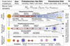 |
Fig. 1 Bern Model: schematic diagram (not drawn to scale) illustrating the breadth of physical processes incorporated in the Generation III Bern Model of Planet Formation and Evolution. Panels a and b show the fixed and varying initial conditions, respectively. The physical processes relevant to the protoplanetary disk are indicated in panel c. It represents a snapshot of the starting point of the model: several protoplanetary embryos are embedded in a disk of gas and planetesimals. The processes that govern planet formation and evolution are displayed in panel d. In panel e, additional physics incorporated in the model is shown. The arrows indicate the evolution of a fixed mass star. Most of the depicted physical processes occur simultaneously and not all processes are shown. See text for summary and Paper I for details. |
2.2 Planet formation
In core-accretion models, planet formation occurs in two major steps. Initially all embryos grow by accreting planetesimals at a rate of ~ 10−5 M⊕ yr−1, while the rate of gas accretion is very low (Alibert et al. 2005; Pollack et al. 1996). Eventually, the protoplanetary gas becomes gravitationally bound to these growing planetary cores. If the mass of a core crosses a certain critical mass threshold (~ 10 M⊕) while the nebular gas is still present, it can undergo runaway gas accretion and becomes a giant planet (over a few million years). In contrast, planetary cores failing to cross the mass threshold do not undergo runaway gas accretion. Accreting solids from their feeding zones, these cores undergo collisions with other cores and result in a diverse range of planets (over ≈10–100 Myr) (see panel d of Fig. 1). The implementation of solid and gaseous accretion is described in Appendix B.2.
2.3 Additional physics
The Bern Model considers several additional physical mechanisms (see panel e of Fig. 1).
Orbital Migration
Gravitational interactions between the planet and the disk lead to the orbital migration of planets and the damping of eccentricity and inclination. The exchange of angular momentum via torques usually results in an inward migration of planets. Low-mass planets undergo type I migration, which is implemented following the approach of Coleman & Nelson (2014) and Paardekooper et al. (2011). Massive planets can open a gap in the gas disk and undergo type II migration, which is implemented following Dittkrist et al. (2014). In type II migration some planets can migrate outwards. Planets inside the gap, if detached, continue to accrete until the disk disappears (Kley & Dirksen 2006).
N-body interactions
Gravitational interactions between the star and multiple planets are included through the N-body code mercury (Chambers 1999). This formation stage tracks the dynamical evolution of planetary orbits, resonances, and collisional growth of planets (Alibert et al. 2013). Orbital migration and damping are coherently included in the N-body. The N-body computations are performed for 20 million years from the start of the model.
After N-body
The model calculates the internal structure of all planets for 10 billion years, after which calculations are stopped. This stage includes effects like atmospheric escape (Jin et al. 2014), bloating (Sarkis et al. 2021), and tidal migration.
2.4 What is meant by the radius of a planet?
In the Bern Model, all planets have a spherically symmetric structure composed of several layers of accreted material. These layer are the iron core, silicate (perovskite MgSiO3) mantle, and water ice (if accreted) for the planetary core, and a H–He gaseous envelope (if accreted). For planets without any gaseous envelope the radius is obtained by solving the core internal structure (see Paper I). In this study, core radius and radius are used interchangeably for such planets.
Planets with gaseous envelopes, however, do not offer a well-defined surface. The radius of such planets depends on the wavelength at which transits are measured (Heng 2019). To facilitate comparison with transit observations, in this work the concept of transit radius is used. Transit radius is the radial distance from the centre of a planet, where the optical depth for a visible ray of light grazing the planet’s terminator (chord optical depth) is 2∕3 (Burrows et al. 2007; Guillot 2010). In this study transit radius and radius are used interchangeably for such planets.
3 New generation planetary population synthesis
Population synthesis provides a way to compare theory with observations of exoplanets and their architecture at the population level (Ida & Lin 2004; Mordasini et al. 2009). The framework of population synthesis rests on one key assumption: the rich diversity in nature’s exoplanetary population emerges due to a variety of possible initial conditions and N-body interactions (Benz et al. 2014; Mordasini 2018). Thus, multiple runs of a global model (while varying the initial conditions for disk and star, and including N-body interactions) can produce theoretical exoplanetary populations possessing some of the observed diversity. Panels a and b of Fig. 1 show the fixed and varying initial conditions.
The New Generation Planetary Population Synthesis (NGPPS) consists of synthetic planetary systems computed from the generation III Bern Model (see Paper II). The Bern Model simulates planet formation and evolution by following the simultaneous growth of multiple planetary embryos embedded in a protoplanetary disk. However, since the number of embryos in a disk is unknown, it is treated as a free parameter. In this work three nominal models are studied with 20, 50, and 100 embryos. Each model is used to simulate 1 000 planetary systems, wherein different initial conditions are assigned to each system in a Monte Carlo manner9. The following Monte Carlo variables are used (for details see Paper II):
Initial mass: Protoplanetary gas disk, Mg
The initial distribution of gas disk mass, Mg, follows the mass distribution of Class I disks reported by Tychoniec et al. (2018). The values range from 0.004 M⊙ to 0.16 M⊙. This governs the initial spatial distribution and surface density profile of the disk via Eq. (B.3).
Disk lifetime: photo-evaporation rate, Ṁwind
Varying Ṁwind allows the model to have disks with different lifetimes. Disk lifetimes closely follow the observed disk lifetimes (see details in Paper II).
Stellar metallicity: dust-to-gas ratio, fD/G
The initial mass of the solids in the disk is a fraction of the initial mass of the gas disk Mg (dust-to-gas ratio, fD/G). Varying thisratio allows the model to capture the observed variation in stellar metallicities. This assumes the relation
![Mathematical equation: \begin{equation*}10^{[\text{Fe/H}]}\,{=}\,\frac{f_{\textrm{D/G}}}{f_{\textrm{D/G},\odot}} \ \text{, } f_{\textrm{D/G},\odot}\,{=}\,0.0149 \text{ \citep{Lodders2003}.} \end{equation*}](/articles/aa/full_html/2021/12/aa40761-21/aa40761-21-eq1.png) (1)
(1)
The distribution of metallicities is in the range −0.6 to 0.5 and follows that of Santos et al. (2005). Additionally, it is assumed that all of the dust in the solid disk is converted to planetesimals10.
Inner edge of disk, rin
Regions of the disk that are close to the star interact with the stellar magnetic field resulting in stellar accretion, ejection, outflows, among other phenomena. The inner edge of the disk is taken at the co-rotation distance from the star, which is the distance where the Keplerian orbital period matches the rotation period of the star. The stellar rotation periods are sampled from observations (Venuti et al. 2017). The distribution has a mean value of 4.7 days (corresponding to 0.055 au), while the lower end is truncated at 0.77 days.
Initial location of planetary embryo, aembryo
Planetary embryos are initialized with a mass of 10−2 M⊕. The initial location of embryos follows a distribution that has a uniform probability in the logarithm of distance between rin and 40 au. It is ensured that all embryos are at least 10 RH apart from each other, resulting from their runaway growth (Kokubo & Ida 1998, 2002).
The characteristics of all NGPPS planetary systems are strongly distorted by failed embryos due to their tremendous numbers. As a working definition, planetary embryos that fail to grow more than ten times from their initial masses are considered failed embryos. To simplify the discussion that follows, failed embryos are removed from the underlying population by removing objects with mass below 0.1 M⊕11. In addition, for simplicity, only the results of the 100-embryo population are presented (except in Sect. 8.2 where the 20- and 50-embryo populations are also discussed).
Synthesizing thousands of planetary systems using the Bern Model, from a human perspective of current standards, is a theoreticallycomplicated and numerically expensive endeavour; however, it is only a simplified approximation of our current understanding for how nature forms planets and planetary systems. The simplifications, choices, and assumptions made in the model may have a strong impact on the outcome of this study. Some of the major caveats are mentioned here, and the details can be found in Paper I (for the model) and Paper II (for the population synthesis). The model assumes planets form via core accretion and ignores other formation pathways like disk instability. The protoplanetary disk and the internal structure of planets are solved via 1D models which may not capture the nuances of 3D effects. The model assumes that the time required for forming protoplanetary embryos is negligible compared to the evolution timescale of the gaseous disk, and that all embryos undergo the oligarchic growth regime. The dust-to-gas ratio of the disk is assumed to be the same as that of the star, and all the dust in the disk is assumed to aggregate into planetesimals (rocky or icy) of fixedsize and fixed densities. The N-body interactions are tracked for only 20 Myr which may not be enough to capture dynamical effects, collisions, or instabilities beyond 2 au. Merger collisions and stripping of planetary envelopes during giant impacts are treated in a simplified manner. Since the geological evolution of planets is ignored, no secondary Earth-like atmosphere is possible in the current model. Despite these and many other assumptions, the model is remarkably successful in capturing a variety of physics (see Fig. 1) and produces diverse planets and planetary systems which bear impressive resemblance to those found in nature.
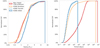 |
Fig. 2 Effect of KOBE: Normalized cumulative distributions for radius (left) and period (right) for the 100 embryo population. The solid red curve represents the underlying population as calculated by the Bern Model. The orange curve is the output of KOBE-Shadows. KOBE-Transits’s pTCE catalogue is shown in light-blue, and the catalogue of planetary candidates, as vetted by KOBE-Vetter is shown in blue. |
4 Kepler Observes Bern Exoplanets (KOBE)
Kepler Observes Bern Exoplanets (KOBE) is a new computer code that simulates transit surveys of exoplanets12. Suppose a population of synthetic planets (as in the Bern Model NGPPS) is hypothetically observed by Kepler’s transit survey. The aim of KOBE in this scenario is to identify those synthetic planets that would have been detected by the Kepler pipeline.
Calculations in KOBE are organized in three sequential modules. KOBE-Shadows, the first module, is tasked with finding transiting planets from a synthetic population of planets. This module produces the KOBE-Shadows catalogue, which consists of systems with at least one transiting planet. All of the planets in this catalogue will transit, but not all of them willbe detected. The next module, KOBE-Transits, computes transit related parameters for transiting planets. Planets that produce a detectable signal are detected. Planets that transit at least two times and have S∕N ≥ 7.1 constitute the KOBE-periodic threshold crossing event (pTCE) catalogue13. The last module, KOBE-Vetter, applies the completeness and reliability of the Kepler pipeline by emulating Kepler’s Robovetter (Twicken et al. 2016, 2018; Thompson et al. 2018). Transiting planets that are identified as planetary candidates by KOBE-Vetter make up the KOBE catalogue. The synthetic population in this catalogue is comparable to the exoplanet population discovered by Kepler. Later sections of this paper, analyse the architecture of planetary systems in the KOBE catalogue and compare it to observations. In a forthcoming paper the KOBE catalogue will be compared with other findings of Kepler.
These three modules encapsulate the three different kinds of biases and limitations of a transit survey. KOBE-Shadows accounts for the geometrical limitation of the transit method. A planet can only transit when its orbit is aligned with respect to an observer. KOBE-Transits applies the detection biases coming from physical limitations; large planets in tight orbits around a quiet star are strongly favoured. Finally, KOBE-Vetter imprints the completeness and reliability of a transit survey. In Appendix C the three modules are described in detail.
To understand KOBE’s effect, Fig. 2 presents the 100-embryo underlying population (in red) as it goes through each stage of calculation in KOBE. The shadow catalogue is dominated by planets that have high transit probability (Eq. (C.6)), which is decided mostly by the star-planet distance and to a minor extent by the planet’s size. Therefore, the shadow catalogue closely follows the underlying population in radius, but not in period. The excess of planets in the shadow catalogue around 3 R⊕ comes from a cluster of planets in the underlying population with high transit probability due to their low periods, P < 10 days. As shown in the period distribution,planets with P < 10 days make up 70% of the shadow catalogue, while they account for only 10% of the underlying population.
The pTCE catalogue strongly favours large planets at shorter orbital distances. Therefore, in the radius distribution the tail of small planets in the pTCE catalogue is shifted to right. About 30% of the planets in the shadow catalogue have Rplanet < 1 R⊕, whereas only 10% of the pTCE planets have Rplanet < 1 R⊕. Requiring a minimum of two transits implies that the maximum period of a planet in the pTCE catalogue will be Pmax = (3.5 × 365.25)∕2 ≈ 640 d. This explains the sharp drop at 640 days in the period distribution of the pTCE catalogue. The KOBE-Vetter catalogue closely resembles the pTCE catalogue. Differences arise when the completeness, as emulated by KOBE-Vetter, is considerably low. As seen in Fig. C.2, this occurs for planets with large radii or large periods.
5 KMPS: KOBE multi-planetary systems
In W18 selection cuts were placed to obtain a ‘high-purity’ population of planetary systems, the CKS-Multis (CKSM). The KOBE catalogue described in the last section undergoes similar cuts. Planets with a high impact parameter, b > 0.9, are removed. Planets with multi-transit S∕N < 10 are also removed (defined in Eq. (C.10)). Finally, planetary systems with only one remaining planet are removed. This creates a catalogue of KOBE’s multi-planetary systems (KMPS), which have the same characteristics as the CKSM catalogue coming from observations. Figures 3 and 4 present a comparison of the theoretically observed planetary population (KMPS in blue) with observations (CKSM in green) of exoplanets. Overall, the two catalogues have remarkable similarities and understandable differences. The underlying population (Bern Model in grey) is also shown.
The scatter plot in Fig. 3 shows the radius of a planet as a function of its orbital period. It shows that the KMPS and CKSM planetary populations cover similar parameter space. A comparison with the grey points gives an impression of the planets that are missed by the transit method or removed by the selection cuts. In terms of period, the KMPS catalogue is bound by a vertical dashed line. This line marks the maximum period of a planet that can be found by KOBE. This comes from the requirement of at least two transits (ntra is fixed as tkepler∕P). There are two planets in the CKSM catalogue that have periods larger than KOBE’s maximum detectable period, Kepler objects of interest (KOIs) K00435.02 and K00490.02. For a given period, the dotted line approximates the minimum size of a planet that will produce a transit S/N of 10 around a 1 R⊙ star. There are some CKSM planets below this dotted line. These planets are orbiting a star of R⋆ <1 R⊙.
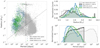 |
Fig. 3 Comparison of planetary populations. Theoretical (blue) represents planets in KOBE multi-planetary systems (KMPS) and observations (green) are the CKS multi-planetary systems (CKSM). Left: Scatter plot with planetary radius on the y-axis and period on the x-axis. The dashed line shows the maximum period of a planet that can be found by KOBE. The dotted line shows the minimum radius of a planet around a 1 R⊙ star for producing a transit S/N of 10. The underlying theoretical population is shown in grey. Right: Comparison of radius (top)and period (bottom) distributions. The radius valley can be clearly seen in the planets found by KOBE and the California-Kepler survey. |
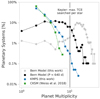 |
Fig. 4 Distribution of planetary multiplicity: Bern Model in grey, Bern Model detectable planets (P < 640 days) in black, KMPS in blue, and observed CKSM in green. The solid black line indicates the maximum number of TCE searches for a star performed by the Kepler pipeline. |
5.1 Radius and period distributions
For radius (Fig. 3) the KMPS and CKSM populations are quite similar. The KMPS radius distribution shows the cumulative effects of both KOBE and the selection cuts placed on the underlying population. This distribution shows a bimodal nature with the two modes being around 1.4–1.7 R⊕ and 2–3 R⊕. The observed CKSM radius distribution also shows this feature. This is the well-known radius gap seen around 2 R⊕ (Fulton et al. 2017; Venturini et al. 2020). The CKSM population has more planets with sizes between 3 and 4 R⊕ than the KMPS population. This can be attributed to a dearth of 3–4 R⊕ planets withP < 100 days in the underlying population. This is also reflected in the sharp drop seen in the period distribution of KMPS planets with P ≈ 100 days. The radius distribution of the underlying populations, however, does not show a radius gap. This is because the underlying population is dominated by small planets at a large distance from the host-star. It is the cumulative effect of applying transit probability (via KOBE-Shadows) and the detection biases of the transit method (via KOBE-Transits and KOBE-Vetter) that removes these small and distant planets. This allows the radius valley in the theoretical population to be clearly seen.
The period distributions of the KMPS and the CKSM populations have similar slopes after their respective peaks. This is a reflection of the role played by transit probability (which decreases as P−3∕2). In the KMPS population the period distribution peaks at about 3 d, while the CKSM distribution peaks around 5 days.
5.2 Multiplicity distribution
The geometrical limitations of the transit method severely impacts the observed multiplicity of planets in a system. Multiplicity, for an observer, results from the overlap of transit shadow band of multiple planets at the observer’s location (see Fig. C.1). Low mutual inclination between multiple planets leads to a large overlap in the transit shadow bands. This results in a higher probability that observers will find multiple transiting planets. The mutual inclination of planets is governed, in part, by the dynamical history of the system. Figure 4 shows the multiplicity distribution. The theoretical KMPS population shows a noteworthy similarity with the observed CKSM population. The vertical solid black line indicates the maximum number of TCEs per star that was searched by the Kepler pipeline (Twicken et al. 2016). The multiplicity distributions of the KMPS and CKSM populations show large differences with the underlying synthetic populations. This is directly attributed to the geometrical limitations inherent in the transit method.
About 60% of the systems in the CKSM catalogue have only two planets. The percentage of systems with higher multiplicity drops sharply, with less than 1% of CKSM systems having six or seven planets. The KMPS catalogue closely follows the CKSM catalogue in the multiplicity distribution. KMPS systems with two planets are less frequent than CKSM systems (about 50%). However, for three or more planets the KMPS catalogue has more systems than the CKSM catalogue. This may arise due to the low mutual inclination between the planets formed in the Bern Model (Mulders et al. 2019).
6 Peas in a pod
The so-called peas in a pod trends in the architecture of planetary systems refers to correlations observed in the properties of adjacent exoplanets. The following statements define the peas in a pod trends in the architecture of multi-planetary systems:
Size: planets within a system tend to be either similar or ordered in size. Here, similarity implies that for two adjacent planets Router∕Rinner ≈ 1. Two adjacent planets are said to be ordered in size when the outer planet is larger than the inner planet, Router∕Rinner > 1;
Mass: planets within a system tend to be either similar or ordered in mass. Here, similarity and ordering are defined using a planet’s mass;
Spacing: for systems with three or more planets the spacing between a pair of adjacent planets is similar to the spacing between the next pair of adjacent planets. This is quantified by the ratio of period ratios for adjacent pairs of planets, (Pj+2∕Pj+1)∕(Pj+1∕Pj) ≈ 1. The index j identifies different planets, where j = 1 is the innermost planet;
Packing: small planets are found to be closely packed together, while large planets tend to have large orbital spacing. This is quantified by comparing the average radii of adjacent planets (Rinner + Router)∕2, with their period ratio Pouter∕Pinner.
These statements take the results from W18 and Millholland et al. (2017) into account. These trends were examined in W18 by measuring the strength of correlations using the Pearson R correlation test. Since the aim of this paper is to examine the architecture trends, the same correlation test is used throughout this paper to compare the correlation between synthetic planetary systems and observations14. We note that correlation coefficients can only measure the strength of correlation in one dataset and that they cannot measure the similarity between two underlying datasets (see Bashi & Zucker 2021 for an inter catalogue similarity metric). In addition, since correlation coefficients require large datasets, they cannot be used to measure architecture trends for a single system.
Figure 5 presents a comparison of the correlation coefficient found in the observed exoplanetary systems (CKSM) and the observable synthetic population (KMPS). There is a remarkable agreement in the correlations of size and packing. Although present in KMPS, the spacing correlations are not as strong as those found in CKSM. As transit observations do not yield planetary masses, the correlation coefficient for mass is not available for the CKSM systems. Each panel in Fig. 5 is discussed below with additional details.
 |
Fig. 5 Peas in a pod. Comparison of the correlations present in the theoretically observed KMPS catalogue (theory) and the CKSM catalogue (observations). Also shown are the correlations present in the underlying Bern Model population (grey). |
6.1 Peas in a pod: radius
Following W18, before testing for correlations in size (and also in mass), all adjacent pairs of planets in the KMPS population are required to undergo a swapping test. If both planets in a pair produce transit S∕N ≥ 10 (see Eq. (C.10)) when their orbital positions are swapped, then this pair is included for testing correlations. Figure 6 shows the radius of an outer planet as a function of the inner planet’s radius, for the underlying (left) and the KMPS (right) populations.The middle panel shows the same for planets from the underlying population that could have been detected by KOBE (P <640 days).
For the KMPS population there is a strong (Pearson R = 0.64) and significant correlation present in the size of adjacent planets15. The size correlation between adjacent planets is also seen through the Spearman R test (Spearman R = 0.69). This impliesthat adjacent planets in the KMPS catalogue have sizes that are similar to their neighbours. The plot also shows that for 65% of adjacent pairs the outer planet is also the largest planet. This frequency of ordered adjacent pairs in KMPS is exactly the same as seen in CKSM (W18) and similar to the findings of Ciardi et al. (2013). This implies that the outer planet in an adjacent pair of planets is often the larger planet in the KMPS catalogue.
It is interesting to compare the size correlations present in the KMPS populations, with the size correlations present in the underlying populations. The underlying population (Fig. 6 (left)) shows strong (Pearson R = 0.66, Spearman R = 0.64) and significant (p-value ≪ 10−10) correlation in size of adjacent planets. This is an important result, and it strongly suggests that size correlation between adjacent pairs of planets is already present in the underlying population. However, only 48% of the pairs in the underlying population are ordered.
Keeping only detectable planets (with P < 640 days) shows the size-correlation present in the underlying population of detectable planets. Compared to the entire underlying population, this population shows a stronger size similarity and size ordering. Removing non-detectable planets tends to remove many small planets that occur frequently in the outer parts of a system. However, adjacent pairs where the outer planet is smaller are removed more often than the adjacent pairs where the outer planet is larger. This shows that the inner region of many planetary systems is populated by size-ordered pairs. This also explains the increase in size correlation seen in this population, which arises from a decrease in adjacent pairs where the outer planet is smaller.
The role of detection biases becomes clear when the KMPS population is compared with the population of detectable planets. Since, small planets are harder to detect via the transit method, many planets with Rplanet < 1 R⊕ are not found by KOBE. This effectively decreases the size-similarity correlation. However, as the KMPS population is a subset of the population of detectable planets, it inherits the frequency of size-ordered pairs.
Overall, the theoretically observed KMPS catalogue shows similarity and ordering in the size of adjacent planets. These trends are in excellent agreement with observations. The theoretical underlying population of detectable planets also shows these correlations. While the size similarity and size ordering are affected by the detection biases, these correlations do not originate from detection biases of the transit method. This suggests that the correlations seen in observations may have an astrophysical origin.
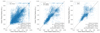 |
Fig. 6 Peas in a pod: size. The sizes of adjacent planets are shown for the underlying population (left), for the underlying population of detectable planets (P < 640 days) (middle), and for theoretical observed planets (right). |
6.2 Peas in a pod: mass
Figure 7 shows the masses of the inner and outer planets in an adjacent pair. For the KMPS population a swapping test as described in Sect. 6.1 was implemented. There is a strong and significant correlation present between the masses of adjacent pairs of KMPS planets. These correlations are also confirmed by the Spearman correlation test. This impliesthat adjacent planets in the KMPS populations have similar masses. Figure 7 also shows that about 55% of KMPS adjacent pairs lie above the y = x line (i.e. they are ordered in mass). This means that there are more planetary pairs where the outer planet is also the more massive planet.
Whether this trend is also present in the underlying population is an interesting question. Figure 7 (left and middle) shows that the underlying population have an even stronger and significant mass similarity correlation.In the underlying population, the outer regions of a system are heavily dominated by small planets with Mplanet < 1 M⊕. When the population of detectable planets is considered, these small planets are noticeably missing (Fig. 7 (middle)). In addition, mass-ordered adjacent pairs are more common in the inner region of many planetary systems. Thus, as noted in thelast section, considering only detectable planets has two important consequences: increase in mass similarity correlation and increase in frequency of mass-ordered planetary pairs. This suggests that detectable planets in the Bern Model tend to have masses similar to their adjacent neighbour or that the outer planet in an adjacent pair is often the more massive planet.
Overall, adjacent planets in the KMPS catalogue show mass similarity and ordering. Since mass similarity and ordering are already present in the underlying population of detectable planets, these correlations do not emerge from the detection biases of the transit method. This implies that the peas in a pod mass similarity and mass ordering trend is probably astrophysical in origin. However, detection biases seem to diminish the strength of these correlations (see Sect. 7).
The patterns seen in the mass trend are strikingly similar to the size trends discussed above. This suggests that the two trends may not be independent of each other. This is understandable since the size of a planet strongly depends on its mass. Planetary mass is evaluated directly from formation physics, whereas the planetary radius has to be evaluated from additional considerations.
Figure 8 shows a mass-radius diagram of all planets in the KMPS 100 embryo population. Planets with a large envelope mass fraction are composed mainly of H–He gases that they accreted during their formation. On the other hand, planets with a low envelope mass fraction are mostly dominated by their cores and have a small H–He gas envelope. The plot shows that Jupiter-sized planets have high envelope mass fractions, while planets with sizes < 4 R⊕ are mostly core-dominated. The high value of the Spearman correlation coefficient (R = 0.81) indicates that the radius as a function of planetary mass is a highly monotonic function16. This implies that for the KMPS planets an increase in planetary mass is very likely to result in an increase in the planetary radius as well.
These factors suggest that the trends of planetary masses are probably more fundamental in the system architecture. The trend seen in the size of adjacent planets is likely to be a derivative trend from the mass correlation.
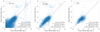 |
Fig. 7 Peas in a pod: mass. The masses of adjacent planets are shown for the underlying population (left), for the underlying population of detectable planets (P < 640 days) (middle), and for theoretical observed planets (right). |
6.3 Peas in a pod: spacing
To investigate the correlation in spacing between adjacent pairs of planets (for systems with three or more planets) the ratio of periods are used. Figure 9 shows the period ratio for an outer pair of adjacent planets Pj+2 ∕Pj+1 as a function of the period ratio of an adjacent inner pair of planets Pj+1 ∕Pj. Following W18, the period ratios are limited to 417.
The correlation tests reveals that there is a positive correlation for spacing in the KMPS catalogue (R = 0.25). The observed CKSM catalogue showed even stronger spacing correlation with R = 0.46 (W18). The underlying population shows a much stronger (R = 0.55) and significant correlation. This implies that for the theoretically observed and underlying population, the period ratio of one pair of planets is correlated with the period ratio of the next pair of planets. However, this trend is notably diminished when the underlying population is analysed by KOBE (discussed further in Sect. 7.2).
The plots in Fig. 9 shows that many pairs of planets are found in orbital mean motion commensurability. The dashed horizontal lines are shown to guide the eye for some of the important commensurabilities. The number in brackets is the percentage of outer planetary pairs that have a period ratio within 1% of the indicated commensurability. For example, in the KMPS 100-embryo population, about 14% of outer planetary pairs are in the 3∕2 orbital commensurability, and 11% and 10% of planetary pairs are close to the 4∕3 and 2∕1 commensurability, respectively. With a period ratio of 1∕1 there are also some cases of co-orbital commensurabilities (Leleu et al. 2019).
The spacing correlation increases sharply as the number of embryos increases in the underlying populations (not shown). The introductionof more embryos in a system has several consequences. Most importantly, it increases the dynamical interactions between growing embryos and planets causing more merger collisions and ejection of planets. In addition to creating new planetary neighbours, these scenarios also lead to a dynamical clearing of space. For example, if three consecutive planets in a system have periods 1, 10, and 100 days, respectively, then all adjacent pairs have a period ratio of 10. The ejection of the middle planet creates new adjacent pairs with a period ratio of 100. If multiple planets, within a system, are clearing space through dynamical interactions, then this provides a mechanism for adjacent planets with correlated spacing to emerge. In Sect. 8.2, the effects of dynamical interactions are analysed further.
Figure 9 also shows that the frequency of spacing ordered adjacent planetary pairs (i.e. where the period ratio of the outer pair is larger than the inner pair) is always less than 50%. This suggests that it is more common to have larger spacing between the inner pair of planets for any three consecutive planets. This frequency decreases with increasing the number of protoplanetary embryos (not shown). This also suggests that increasing dynamical interactions plays a role in allowing adjacent planetary pairs with larger spacings to emerge.
The frequency of ordered adjacent pairs falls sharply for the population of detectable planets. This indicates that for three consecutive planets an inner pair that has a larger spacing than an outer adjacent pair is much more common in the inner region of a system. This could, potentially, be a result of limited N-body calculation time. In NGPPS the N-body calculations are done until 20 Myr. This means for a planet located at 1 au or 365 days that the N-body tracks its evolution for 20 M orbits. For planets that are further out their orbital evolution is tracked for lesser number of orbits, which could thereby influence the results.
In the context of spacing between adjacent planets, another possibility to explore is the role played by the initial location of embryos (described in Sect. 3). A simple calculation allows us to derive the expected value of initial period ratio of embryos by converting uniform log spacing in semi-major axis aembryo to periods:
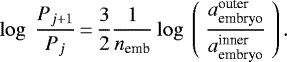 (2)
(2)
Here, nemb is the total number of embryos initially placed in a simulation and the factor 3∕2 comes from the application of Kepler’s third law, and  is the maximum distance from the star at which an embryo can be placed. For the inner edge the mean value of rin = 0.055 au can be used. This provides an approximate value of the average initial period ratio of embryos. The value of this is 1.6, 1.2, and 1.1 for the populations with 20, 50, and 100 embryos respectively. This implies that all planetary embryos start with period ratios close to 1. While the initial period ratios of embryos is close to unity, the location of an embryo is assigned randomly (see Sect. 3). This would result in the absence of the spacing correlation at early times (see Fig. 12). It is clear from the plot that there is little trace of these initial values at 4 Gyr.
Overall, all theoretical populations show a positive spacing correlation in agreement with observations. The spacing between one pair of planets is similar to the spacing between the next pair of planets. The large correlations present in the underlying population suggest that this trend is probably astrophysical in origin. Geometrical limitations and detection biases have a noticeable influence on the spacing correlation (see Sect. 7). For synthetic populations,the period ratio of an inner pair of planets is often larger than the period ratio of the next outer pair.
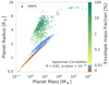 |
Fig. 8 Mass–radius relationship. Planetary radii are plotted as a function of planetary masses for the planets in the KMPS 100-embryo population. For planets with non-zero H–He envelopes, the colour denotes their envelope mass fraction,
|

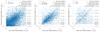 |
Fig. 9 Peas in a pod: spacing. The plots shows the period ratio of the outer pair of planets as a function of the period ratio of the inner pair for the underlying population (left), for the underlying population of detectable planets (middle), and for the KMPS systems (right). The dashed horizontal lines mark some of the important commensurabilities. The number inside the parenthesis is the percentage of outer planetary pairs that have a period ratio within 1% of the indicated commensurability. |
6.4 Peas in a pod: packing
Weiss et al. (2018) have found that smaller planets tend to have small spacing while larger planets are likely to have large spacing. There is a correlation between the average size of an adjacent planetary pair with their period ratio. The Pearson correlation coefficient for the packing trend in the CKSM catalogue is R = 0.26.
It is suggested in Sect. 6.2 that the correlations seen in sizes probably arise from underlying correlations present in planetary masses. The correlations in planetary masses are probably more fundamental than those of planetary radii. A further test of this idea could be if the packing correlations were to also exist in planetary masses. This has not been reported in the literature before. Figure 10 shows the average size (top) and average mass (bottom) of adjacent pairs of planets as a function of their period ratios Pj+1∕Pj.
For the KMPS population the Pearson correlation coefficient for the packing trend (with average sizes) is R = 0.23, which is in good agreement with observations. The plot shows that for planetary pairs of average size 1 R⊕, the spacing is generally lower than pairs of average size 2 R⊕. The correlation stems from the lack of planetary pairs with small average sizes and large spacing between them. Figure 10 (top left) shows that this correlation is even stronger in the underlying population. Here the correlation coefficient is R = 0.45. The plot shows that while there is a cluster of points with low period ratios (Pj+1∕Pj < 2) extending from average sizes 0.5 to 5 R⊕, the correlation seems to emerge from the lack of small planetary pairs with large spacing. For example, there is only one pair of adjacent planets in the underlying population with average size between 1–2 R⊕ and period ratio between 128 and 512. For the same period ratio bin, there are two pairs of planets with average sizes between 2–4 R⊕, while there are eight pairs of planets with average sizes between 4 and 8 R⊕.
Figure 10 (bottom) shows that the average mass of planetary pairs is indeed correlated with their spacing. The correlation of period ratios is stronger with average mass than with average size. The correlation coefficient is R = 0.26 for the KMPS population and increases to R = 0.57 for the underlying population. These plots show features that are similar in quality to the plots with average sizes. For all populations there are no planetary pairs with average mass >1000 M⊕ and spacing Pj+1∕Pj < 3∕2. This can be explained by invoking stability arguments. Deck et al. (2013) studied long-term stability of planetary systems and provided stability criteria. The Hill stability criteria (Eq. (59) from their paper), relating masses and locations of two planets, is plotted in Fig. 10. A pair of planets are Hill stable if they are on the right side of the black curve.
To further understand the packing trend, the location of the inner planet (in an adjacent pair) is shown in colour for the underlying population. The coloured plot shows several interesting features. This trend is mostly driven by planetary pairs where the inner planet is located close to the host star (P ≲ 10 days). For these pairs of planets the spacing seems to increase with their average size and mass.
As mentioned in Sect. 6.3, dynamical interactions can lead to merger collisions and ejection of planets. This results in dynamical clearing of space between planets. Large planets may undergo several collisions leading to the ejection or accretion of several planets. This may allow them to have wider orbital spacing. On the contrary, small planets may not have undergone several collisions, thereby remaining in compact configurations. This could explain how small planets tend to have smaller orbital spacing and large planets have wider orbital spacing. Due to limited N-body integration time, the inner region (<1 au/365 days) of a planetary system experiences many more dynamical interactions than the outer region. This explains the small contribution towards the packing trend from planets that are in the outer region (green points). This scenario is discussed further in Sect. 8.2.
Overall, the findings of this section indicate that the average mass (and therefore the average size) of a planetary pair is correlated with their spacing. Planets with smaller masses are packed closely together, while massive planets seem to have larger orbital spacing between them. As these correlations are also present in the underlying population, it hints towards an astrophysical origin of this trend. In W18 this trend was further examined through the mutual separation (Δ) of adjacent planet in units of mutual Hill radius. Their findings can be explained by detection biases, and is discussed in Appendix A.
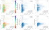 |
Fig. 10 Peas in a pod: packing. The average sizes (top) and average masses (bottom) of adjacent planets are shown as a function of their orbital period ratios Pj+1 ∕Pj for the underlying population (left), underlying population of detectable planets (middle), and KMPS planets (right). For the underlying population, the position of the inner planet in each pair is in a different colour, showing that the trend is due to those planetary pairs where the inner planet is close to the host star. The black curveshows the Hill stability criterion from Deck et al. (2013). Adjacent planetary pairs on the right side of this curve are Hill stable. Points on the left side are Hill unstable and will probably be removed with longer N-body calculations. |
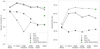 |
Fig. 11 Influence of the geometrical limitations of the transit method (KOBE-Shadows), the transit detection biases (KOBE-Transits), and the completeness of the Kepler survey (KOBE-Vetter) on the peas in a pod trend. The plot shows how the correlation coefficients (left) and the frequency of ordered pairs (right) varies in the underlying Bern Model population, the underlying population of detectable planets (P < 640 days), and the theoretically observed KMPS population (for the size–mass trends in the KMPS catalogue adjacent planetary pairs have undergone a swapping test, as mentioned in Sect. 6.1). Observations from the CKSM exoplanetary catalogue are shown in green. |
7 Role of detection biases in peas in a pod trend
Population synthesis based on planet formation models provides a natural playground for testing the role of detection biases of the transit method in the peas in a pod trends. The Bern Model consists of theoretical description for many physical phenomena that are active during planet formation. Supplying them with randomized initial conditions and N-body calculations, the NGPPS provides a theoretical version of nature’s underlying population. The KMPS catalogue, from KOBE, stands on the same footing as observations (CKSM). This work thus allows both the theoretically observed exoplanetary populations (from KOBE) and the theoretical underlying populations (from NGPPS) to be investigated for the peas in a pod trend.
To understand how the geometrical limitations and the detection biases of the transit method affect the peas in a pod trends, the correlation test was performed after each stage of calculations in KOBE. Figure 11 (left) shows the Pearson correlation coefficient for the similarity trends in size, mass, spacing, and packing. Figure 11 (right) shows the percentage of ordered pairs for size, mass, and spacing18. Observations from CKSM are in green.
The similarity and the differences of these trends can be understood via the following statement. The chances of detecting a transiting exoplanet depend strongly on its location (star–planet distance and orbital period) and weakly on its size (radius). Specifically, the size dependence is from Rplanet∕R⋆ (see Eq. (C.6)), which varies from 10−3 for sub-Earth-size planets to 10−1 for Jupiter-size planets around a Sun-like star. This suggests that the effect of geometrical limitations and detection biases will be much more severe on orbital periods than on planetary sizes. This is easily seen from the plots in Figs. 2 and 11.
7.1 Peas in a pod: mass and size
One strikingfeature in Fig. 11 is that the size trend closely follows the mass trend. The small variations between the two trends probably arise from the scatter seen in the mass-radius diagram (see Fig. 8). The underlying population shows strong mass (and thereby size) similarity and ordering correlations. This strongly indicates that the peas in a pod mass (and thereby size) trend arises from planet formation.
The geometrical limitations and detection biases of the transit method tend to decrease the strength of the similarity correlations. The vetting procedure, in KOBE-Vetter, seems to have little effect on the mass (size) similarity correlations. Although the completeness of Kepler’s Robovetter drops sharply with radius (see Fig. C.2), the frequency of large planets in the KOBE-Vetter catalogue is also low: about 70% of planets have Rplanet ≤ 3 R⊕. Finally. the size correlations seen in the KMPS catalogue match the observations very closely.
However, KOBE has little influence on the mass–size ordering trend. For the underlying population of detectable planets, the frequency of mass–size ordered pairs is close to 60%. This means that there is a higher chance for an outer planet in a pair to be heavier and/or larger. The frequency of size-ordered pairs in KMPS matches CKSM observations very closely.
Since the size-similarity and ordering trend in the KMPS populations very closely matches the observations, one could extrapolate this to learn about the nature of the underlying exoplanetary population. These results suggest that the size–mass similarity and ordering correlations found in observations are probably astrophysical and are not severely affected by detection biases.
7.2 Peas in a pod: spacing and packing
The underlying populations shows strong spacing (for systems with three or more planets, period ratios limited to 4) and packing trends. Both of these trends involve period ratios of adjacent planets, already hinting that these trends will be strongly influence by KOBE. One way in which KOBE influences the spacing and packing trends is due to missing planets.
KOBE-Shadows finds transiting planets that have a fortuitous alignment with an observer. Transiting planets found by KOBE-Shadows are not necessarily consecutive. In several cases many intermediate planets are missed, resulting in a strong affect on period ratios. However, the effect of missing planets may be more adverse on the packing trend than on the spacing trend. Consider a hypothetical system with five planets at periods of 1, 10, 100, 1000, and 10 000 days. The period ratio for all four adjacent pairs is 10, and the ratio of period ratios for any three consecutive planets is 1. If the planets with periods of 10 and 1000 days do not transit for an observer, then the period ratios of the two transiting adjacent pairs jumps to 100. However, for the three transiting planets the ratio of their period ratios is still 1. If the two transiting adjacent planets have small average sizes, then the jump in the period ratio will weaken the packing correlation. This example demonstrates the adverse effect of missing planets on the packing trend19. This explains the diminishing of the spacing trend and the absence of packing correlation from the 100-embryo population in the KOBE-Shadows catalogue.
KOBE-Transits requires that all transiting planets have at least two transits, which implies that only planets with P < 640 days can be included.This means that only the inner region of a planetary system is now considered. This helps in removing pairs with abnormally high period ratios caused by missing planets. This may explain how the packing trend is restored in the catalogue from KOBE-Transits. The spacing trend is reduced further by KOBE-Transits and KOBE-Vetter. These modules provide imprints of the physical detection biases and completeness profile of the Kepler pipeline.
The role of adding biases on the spacing ordering trend can be seen in Fig. 11 (right). For the underlying population the frequency of ordered pairs is less than 50% (for three consecutive planets there are more inner pairs with larger spacing than their next outer pair). There seems to be little influence of KOBE, and thereby detection biases, on the frequency of ordered pairs.
Overall, the underlying populations show strong spacing and packing trends. Geometrical limitations and detection biases of the transit method are responsible for reducing the strength of these correlations.
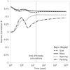 |
Fig. 12 Evolution of the peas in a pod trends. The vertical solid line represents the end of N-body calculations. |
8 Discussion: theoretical scenarios
The results of Sect. 6 indicate that the peas in a pod trend is present in the synthetic planetary systems from the Bern Model.This section is dedicated to the discussion of some theoretical scenarios that offer partial explanations for these trends.
8.1 The evolution of peas in a pod
One way to understand how the peas in a pod trends emerge is by investigating when the trends emerge. To this end, the correlation tests for all trends were performed for all underlying populations at all time steps. Figure 12 shows the evolution of the correlation coefficients for the underlying 100-embryo population. Since most of the variations happen during the N-body calculations, this suggests that dynamical interactions during the formation stage play a key role in shaping these trends.
The plot shows that the underlying population shows a very strong correlation for the size and mass trends, already at the beginning of the calculations. This suggests that the peas in a pod mass (and thereby size) similarity trends are present at very early times. This high correlation can be attributed to two factors: oligarchic growth of protoplanetary embryos and uniform accretion of solids by protoplanets at early times (see Sect. 2.2). The Bern Model starts with lunar mass embryos that are separated by at least 10 RH. Runaway growth of planetesimals leads to protoplanets, which eventually grow oligarchically. The oligarchic growth stage results in mass ratios approachingunity (Kokubo & Ida 1998). In this way the seeds for the peas in a pod mass trend (and therefore also the size trend) are already planted20. In the Bern Model, protoplanetary embryos accrete solids from the planetesimal disk at a rate given by Eq. (B.6). This core accretion rate prominently depends on the location and mass of the embryo as well as the surface density of the disk,  . Since these factors (surface density of solid disk and location and mass of embryos) do not undergo any drastic changes at early times, the accretion of solids by neighbouring protoplanets is uniform. Thus, uniformly growing oligarchic embryos may explain the high mass–size correlation seen at t = 105 yr in Fig. 12.
Between 105 and 106 yr the correlation coefficient for mass (and thereby size) drops. This could be attributed to the differences in the rate of solid accretion by cores of different types of planets. The cores of giant planets have to reach a critical mass (Mcore ≈ 10–20 M⊕) before the gas disk dissipates (Pollack et al. 1996; Alibert et al. 2005). On the other hand, planetary cores which will fail to reach this critical mass (for runaway gas accretion), are known to have longer formation times (Paper I). When adjacent planetary cores in a system grow at different rates, the correlation between their masses and sizes may decrease. The size correlation seems to trace the mass correlation (with some scatter). That the size trend follows the mass trend is not surprising, since planetary sizes are calculated from their masses (via internal structure calculations).
Between 106 and 2 × 10⁷ yr the correlation coefficient for mass decreases slightly. Most giant planets have acquired their final masses in the first few million years. Other planets, however, continue to grow by solid accretion, gas accretion (before the gas disk dissipates), and merger collisions. This implies that adjacent neighbours may be growing at different rates depending on their local environment. Different growth rates imply that the mass correlation will decrease. The local environment around planets growing in the same disk does not suffer any drastic changes. This may explain why the mass correlation also does not show any drastic changes. Additionally, the dissipation of the gas disk has a strong effect on planetary radii since planets contract rapidly after disk dispersal. This may contribute to the decreasing size correlation in this time period.
The spacing and packing trends start with almost no correlation and undergo interesting variations before ending with their final value. Initially, adjacent planets have uncorrelated small period ratios and small sizes. This may explain the absence of these trends at early times. Some physical processes that affect the location of a planet are orbital migration, resonance capture, and ejection or collision of planets. When a planet is lost (via ejection or collision), it clears up space allowing new adjacent pairs to emerge with wider orbital spacing. This dynamical sculpting may explain how planets within a system evolve towards similar spacing. Large planets may undergo several collisions that lead to the ejection of several planets allowing them to have wider spacings. This offers a possible explanation for the emergence of the packing trend. After a few million years most systems have lost their gas disks, which leads to rapid contraction of planetary radii. This is responsible for the sharp drop in the packing trend (in the range t = 106–2 × 10⁷ yr). As planets continue to grow via merger collisions, the packing trend re-emerges slowly.
The spacing and packing trends are seen to have several common behaviours. They are both absent at early times, arise from dynamical interactions, and are strongly influenced by the detection biases. It is a possibility that these two trends are not independent of each other. In fact there is a simple scenario that could unify them. The peas in a pod spacing trend could be a reflection of the mass similarity and the packing trends. Since adjacent planets are more likely to have similar masses, and the orbital spacing between planetary bodies is related to their masses (heavy planets have wider orbital spacing, while small planets tend to have smaller orbital spacing), the spacing trend can emerge. Planets with large or small masses have neighbours with similar masses, and this leads them to also have period ratios that are similar. Further tests are required to confirm this scenario.
Overall, this section presents two important findings. First, the similarity in mass–size trends are already present at early times. These are, perhaps, due to oligarchic growth of protoplanetary embryos and uniform growth of these protoplanets at early times. Uniformly growing neighbouring planets will continue to show size–mass similarity. Different growth rates amongst adjacent planets during the formation stage tends to decrease the mass–size trends. Second, the spacing and packing trends are absent at early times. Dynamical interactions (especially merger collisions) tend to increase spacing and packing correlations.
8.2 Role of dynamical interactions
Dynamical interactions can often lead to the ejection of planets and merger collisions. This would lead to a decrease in the number of planets in a system. Systems that have had more dynamical interactions will have lost more planets than systems with less dynamical interactions. Since the number of embryos (nemb) that a theoretical system begins with is fixed for each synthetic population, the percentage of lost planets can be used as a diagnostic for its dynamical history. With nmul as the multiplicity of systems at 4 Gyrs, the percentage of planets lost by a system is
![Mathematical equation: \begin{equation*} \mathrm{Lost~planets~[\%]}\,{=}\,\frac{n_{\textrm{emb}} - n_{\textrm{mul}}}{n_{\textrm{emb}}}\,{\times}\,100. \end{equation*}](/articles/aa/full_html/2021/12/aa40761-21/aa40761-21-eq5.png) (3)
(3)
Figure 13 (left) shows the distribution of lost planets in the underlying NGPPS populations. This plot shows that the distribution shifts to the right, as the number of embryos increases from 20 to 50, and from 50 to 100. This demonstrates that adding more embryos in a system tends to increases their dynamical interactions, which in turn forces these systems to lose more planets. This verifies that lost planets can be used as a proxy for the dynamical interactions experienced by a system.
Now the planetary systems are divided into five sub-populations depending on the percentage of planets they lose: [0,20), [20–40), [40–60), [60–80), and [80–100]. The ratio of giant planets to the total number of planets in each system is calculated21. This ratio is then averaged over each sub-population and is shown in Fig. 13 (left). There is a clear increase in the ratio of giant planets in a system with increasing dynamical interactions. This shows that systems with more giant planets have more cumulative dynamical interactions.
For each peas in a pod trend (size, mass, spacing, and packing), the correlation coefficient is measured across each sub-population. This is shown in Fig. 13 (right). As the percentage of lost planets increases, the spacing and packing correlations also increase (for the 50- and 100-embryo populations). This strongly suggests that increasing dynamical interactions results in strengthening of the spacing and the packing trends. This adds support to the finding of the last section that dynamical interactions amongst growing planets leads to the spacing and packing trend. For the 20-embryo population the result of the Pearson correlation test becomes unreliable due to low multiplicities. Going from left to right, the size-mass correlations show little variations at first. However, the size–mass correlations drop sharply in the last two bins. This drop may arise from the presence of giant planets in these sub-populations, indicating an anti-correlation between mass similarity and presence of giant planets.
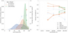 |
Fig. 13 Role of dynamical interactions on the peas in a pod trends. Left: distribution of lost planets [%] by systems in the 20-, 50-, and 100-embryo NGPPS populations. The fraction of planets lost by a system can be used as a proxy for the cumulative dynamical interactions experienced by a system. The dashed lines show the ratio of giant planets per system averaged over bins. Right: correlation coefficient for the peas in a pod trends for each bin. The error bars correspond to the standard error of the correlation coefficient (Zar 2014). Increasing dynamical interactions results in the strengthening of the spacing and packing trend. |
9 Summary, conclusions, and future work
In this paper, the peas in a pod trends in the architecture of planetary systems was studied. Using the Bern Model, thousands of synthetic planetary systems were simulated. To compare this population of theoretical systems with observations, a new computer code, KOBE, was developed and was introduced in this paper.
KOBE closely simulates the geometrical limitations of the transit method and the detection biases of the Kepler transit survey. KOBE-Shadows finds transiting planets via their transit shadow bands, thereby imprinting the transit probability and including the geometrical limitations of the transit method. By selecting only high S/N transiting planets, as calculated by KOBE-Transits, the detection biases of the Kepler mission are simulated. Finally, KOBE-Vetter rejects some of the planets as false positives, emulating the completeness and reliability of the Kepler Robovetter. Transiting planets that are dispositioned as planetary candidates make up the KOBE catalogue.
Additional selection cuts are placed on the KOBE catalogue to generate the KOBE multi-planetary systems population (KMPS). This population is compared with the multi-planetary systems catalogue of the California-Kepler Survey (CKSM from W18). The KMPS and CKSM planetary populations showed similar radius and period distributions. The peas in a pod trend was investigated for several populations. The main conclusions of this paper are:
- 1.
The peasin a pod size and mass similarity trends are present in the theoretically observed (KMPS) and the theoretical underlying (Bern Model) populations. This means that adjacent planets within a synthetic system tend to have similar sizes and masses. The strength of the size trend in the KMPS population is in good agreement with observations. Detection biases tend to diminish the strength of these correlations.
- 2.
The peas in a pod size and mass ordering trends are present in the theoretically observed (KMPS) population. The frequency of size-ordered pairs is in good agreement with observations. This trend is also present in the theoretical underlying population of detectable planets (planets with periods of less than 640 days). Thus, in the inner region of a synthetic system there is a higher chance for an outer planet in an adjacent pair to be larger and/or more massive. Detection biases of the transit method have little influence on this trend.
- 3.
The presence of the size and mass similarity and ordering trends in both the theoretical underlying (Bern Model) and the theoretically observed (by KOBE) populations implies that this trend, also seen in observations, may have an astrophysical origin.
- 4.
The peas in a pod mass–size trends are present at very early times. The primordial origin of these trends is probably due to oligarchic growth of protoplanetary embryos and the uniform growth of planets at early times. Later stages of planet formation, including dynamical N-body effects, allows planets within a system to grow at different rates. This tends to decrease the strength of these trends.
- 5.
In the peas in a pod spacing similarity trend, for three consecutive planets in a system the period ratio of the inner pair tends to be similar to the period ratio of the outer pair. This correlation is present in the theoretically observed (KMPS)and the theoretical underlying (Bern Model) populations.
- 6.
The strength of this trend is higher in the underlying population. Detection biases are responsible for reducing the strength of these correlations. This suggests that the spacing trend, as reported by W18, probably has an astrophysical origin.
- 7.
This trend is absent at early times and likely arises from the dynamical interactions taking place during planet formation stage. Merger collisions and ejection of planets are some of the ways through which planets become evenly spaced. Additionally, this trend increases when the number of embryos in a population is increased, further suggesting that dynamical interactions increase this trend.
- 8.
Observations suggest that large planets tend to have wider orbital spacing, while small planets are often packed in compact configurations. This packing trend is also present in theoretically observed (KMPS) and the theoretical underlying (Bern Model) catalogues. The strength of this trend is in good agreement with observations.
- 9.
Detection biases and missing intermediate planets have a strong influence on this trend. These effects tend to diminish these correlations. However, this trend is likely to have an astrophysical origin since it is also present in the underlying population.
- 10.
This trend is not present at early times and probably arises from N-body dynamical interactions. Large planets undergo several merger collisions, thereby clearing more space around them.
- 11.
The peas in a pod size trends are probably derivative of the peas in a pod mass trends. The existence of mass trends is probably an astrophysical phenomenon. It has also been suggested that the mass similarity and packing trend may combine to give rise to the spacing trend.
The results of this paper imply that physical processes involved in planet formation gives rise to adjacent planets that have similar masses (and therefore sizes), and that are evenly spaced. Large planets tend to have wider orbital spacing, while smaller planets tend to be packed in compact configurations. Detection biases of the transit method diminish the size–mass similarity trends and influence the spacing and packing trend. We suggest that the peas in a pod similarity and ordering trends seen in observations may have an astrophysical origin.
One of the shortcoming of this and other studies on the peas in a pod trends is the use of correlation coefficients in measuring architecture trends. Although useful in making population-level studies, the reliable calculation of correlation coefficients requires large datasets which hinder the study of these trends at the system level. One line of future work could be the development of system level architecture metrics (Alibert 2019; Mishra et al. 2019; Gilbert & Fabrycky 2020). These metrics could allow the architecture of an individual system, the Solar System for example, to be studied. This could allow the disentanglement of the role played by specific initial conditions from the effects of planet formation processes in engendering these trends. Furthermore, system level studies are required to establish the unification of peas in a pod trends, as mentioned previously.
In addition, the present study can be improved by studying different stellar types. To facilitate comparison with W18, several aspects of KOBE were restricted in this paper. For example, the calculation of transit S/N in KOBE assumes that all planets are in circular obits, the sampling of CDPP used fixed value of ttrial = 6h. Future versions of KOBE will include the effect of eccentricity on transit S/N, and will use ttrial values based on calculated transit durations. Additionally, KOBE can be further improved by including stellar limb darkening.
Acknowledgements
The authors thanks the anonymous referee for their comments and suggestions. This work has been carried out within the framework of the NCCR PlanetS supported by the Swiss National Science Foundation. The authors acknowledgesupport from the Swiss National Science Foundation under grant BSSGI0_155816 “PlanetsInTime”. A.E. acknowledges the support from the University of Arizona. Calculations were performed on the Horus cluster at the University of Bern. Data: the synthetic planetary populations (NGPPS) used in this work are available online at http://dace.unige.ch under section “Formation & evolution”. This research has made use of the NASA Exoplanet Archive, which is operated by the California Institute of Technology, under contract with the National Aeronautics and Space Administration under the Exoplanet Exploration Program: https://exoplanetarchive.ipac.caltech.edu (DOI: 10.26133/NEA6). The CKS dataset is available at https://california-planet-search.github.io/cks-website/. Software: KOBE (this paper), Python (Van Rossum & Drake 2009), NumPy (Oliphant 2006), SciPy (Virtanen et al. 2020), Seaborn (Waskom & the seaborn development team 2020), Pandas (pandas development team 2020), Matplotlib (Hunter 2007).
Appendix A Detection biases explain the negative correlation between mutual separation and average sizes and masses
In their effort to study the connection between planetary sizes and their orbital spacing, W18 explored the mutual separation (in units of mutual Hill radii) between planets. The mutual sep- aration between two adjacent planets is defined using their mutual Hill radius  . The mutual Hill radius of two adjacent planets (with masses mj and mj+1) can be thought of as the Hill sphere radius of a single planet located between the two adjacent planets and whose mass is the sum of the two planets. This gives
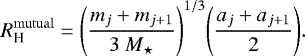 (A.1)
(A.1)
Here, M⋆ is the stellar mass, while aj and aj+1 are the star–planet distances. The mutual separation Δ between two planets is the ratio of their orbital separation to their mutual Hill radius. It measures the dynamical spacing between two planets in units of their mutual Hill radius:
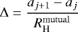 (A.2)
(A.2)
Weiss et al. (2018) find that there is a significant negative correlation between mutual separation and the average size of adjacent planets in the CKSM catalogue (R = −0.2). They state that the mutual Hill radius incorporates the mass of the planet, and thus the computation of mutual Hill radius separation should ideally remove the contribution of planet size. They add that this correlation is driven by an absence of points in the lower left corner of the plot, which means that the absence of very small planets at close dynamical spacings is not due to detection bias.
Here, we show that the dependence of mutual Hill radius on average size is affected by the relationship between mutual Hill radii and mass (through eq. A.1). In addition, since transit surveys detect planets only in the inner region of a planetary system (close to the host star), adjacent planetary pairs with small dynamical spacing will be missing from observations.
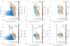 |
Fig. A.1 Dependence of mutual separation of adjacent planets on their average sizes (top) and average masses (bottom). Observed exoplanetary populations (CKSM by W18) show a negative correlation between average sizes and mutual separation of adjacent planets, which is well reproduced here (top left). However, this negative correlation arises from the dependence of mutual Hill radii on the
1∕3 power of planetary masses. This is shown by the dashed line in the plots on the right. The vertical line marks the Hill stability criterion from Chambers et al. (1996). Points on the right side of this line are Hill stable ( |

In Fig. A.1 (top right) the average radius of two adjacent planets (in KMPS) is plotted as a function of their mutual Hill separation. The period ratio of the adjacent planets is shown in colour. In good agreement with W18, there is a significant negative correlation, which is confirmed by a Pearson correlation test (R = −0.1). The bottom plots show the average mass of adjacent planets as a function of their mutual Hill radii. We note that the scatter of points in the top panel closely resembles the scatter of points in the bottom panel. In these plots, adjacent planets of constant period ratios lie on straight lines (i.e. points of the same colour). In the plot with average sizes, adjacent planets of constant period ratios tend to be on straight lines, but show considerable scatter for average sizes > 3 R⊕. This scattercan be traced to the intrinsic scatter in the radius of planets with size > 3 R⊕ in the mass-radius diagram in Fig. 8. The slope of the average mass versus the mutual Hill plot comes from the  power on the mass term in eq. A.1. It gives average masses a slope of − 3 on the log. average mass versus log. mutual Hill plane. To visualize this, the y ∝ x−3 dependence is plotted as a dashed line in Fig. A.1 (right). The slope of this line closely matches the underlying points. This indicates that the incorporation of planet mass in the calculation of mutual Hill radius may influence the relationship between planet sizes and mutual Hill radii.
To test whether this correlation arises from limitations of the transit method, the same correlation test was also done for the theoretical underlying population. Figure A.1 shows the average radius versus mutual Hill separation. The lower left corner of the plot, which was empty for the KMPS population, is filled for the underlying population, but remains empty for the underlying population of detectable planets. This shows that the inner regions of planetary systems do not have planetary pairs with small mutual separation. Since transit surveys can only detect planets in the inner region, this explains why observations will find a negative correlation (which is due to the absence of points in the lower left corner). This suggests that the negative correlation seen in CKSM is probably also due to detection biases and limitations of the transit method. This behaviour is similar to the correlations between average masses and mutual separation.
The question arises regarding why the theoretically observed population (KMPS) or the underlying population of detectable planets shows no adjacent pairs with small size and mass and low mutual separation? This is understandable due to limitations and detection biases of the transit method.
The Hill sphere radius of a planet defines the region around a planet in which the gravitation field of the planet dominates. As the star–planet distance increases, the influence of the star diminishes and RH of a planet increases. This can be seen through eq. B.5. This is also true for the mutual Hill radii,  . As two adjacent planets move further out, their mutual Hill radii increases. The inverse dependence of Δ on
  implies that as the mutual Hill separation between adjacent planets increases, their mutual separation decreases. Thus, adjacent planets in the outer regions of a planetary system will have a large mutual Hill radius and consequently a small dynamical separation. This explains the absence of points in the lower left corner for the plot showing underlying population of detectable planets. Since detection biases of the transit method disfavour the discovery of small planets further out from their host star, it also explains why planets with small average sizes and masses are missing from the lower left corner in the KMPS plots. This provides a plausible explanation for the negative correlation, reported in observations by W18, between mutual separation and average sizes.
Appendix B The Bern Model: Additional details
Additional details of the Bern Model are presented here. First, we describe the physical processes occurring before planets are born. These processes involve the host star and the protoplanetary disk. Then we describe the processes which model planet formation, i.e. the accretion of solids and gases.
B.1 Before planet formation begins
B.1.1 Stellar Evolution
The model includes the evolution of a fixed mass star (M⋆ = 1 M⊙) by incorporating the stellar evolution tracks from Baraffe et al. (2015). The evolving stellar properties influence the behaviour of the disk and the growing planets in multiple ways. For example, stellar irradiation and temperature (L⋆, T⋆) affects the thermodynamical aspects of the disks and the planets. Stellar radius R⋆ strongly affects the transit signal generated by a transiting planet and also allows the tracking of collisions between any object and the star.
B.1.2 Protoplanetary disk: Gaseous phase
The gas disk plays a crucial role in the growth of planets and shaping the planetary system architectures. Accretion of this nebular gas may lead to gaseous envelopes around many planets. Additionally, the gas disk interacts with planetesimals, embryos, and protoplanets through effects such as gas drag, migration, and eccentricity damping.
The model follows the evolution of an axisymmetric geometrically thin gas disk in a time-independent gravitational potential. Gas is accreted by the star and growing planets, and is lost via photoevaporation. Meanwhile, the outer regions of the disk are pushed away to conserve angular momentum until the disk is completely dissipated. The disk evolution is computed in the region from rin up to rmax = 1000 au. Here, r is the radial distance from the star and rin is a Monte Carlo variable for the model (discussed in Sect. 3). The vertically integrated and azimuthally averaged surface density of gas, Σg, evolves as
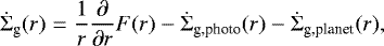 (B.1)
(B.1)
where F is radial flux of gases from viscous angular momentum transport (Lüst 1952; Lynden-Bell & Pringle 1974) 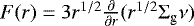 . Effective turbulent viscosity, ν, is parametrized by a dimensionless parameter α as ν= αcsh (following Shakura & Sunyaev 1973)22. Here, cs is the isothermal speed of sound (which depends on temperature and mean molecular mass of gas) and h is the local disk pressure scale height (~ half of disk thickness). Following observations (Manara et al. 2019; Flaherty et al. 2020), in this work α =2 × 10⁻³.
The extreme UV and far-UV radiation from the host star and neighbouring stars, respectively, heat the disk such that thermal motion can overcome gravitational potential resulting in the dispersal of the disk (Clarke et al. 2001; Matsuyama et al. 2003). Following Mordasini et al. (2012b), internal and external photoevaporation losses are included in  . These mechanisms control the disk lifetime via the mass loss rate, Ṁwind, which is a Monte Carlo variable for the model and is discussed in Sect. 3. The disk also loses some amount of gas to planetary accretion, which is represented by
  23.
23.
The model begins with an initial surface density profile for the gas disk given by (Veras & Armitage 2004)
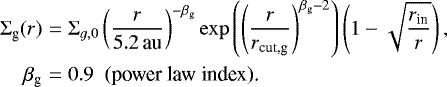 (B.2)
(B.2)
Here, Σg,0 (normalization constant) and rcut,g (characteristic radius) are governed by a Monte Carlo variable, Mg, the initial gas disk mass through the relations (see Paper II):
![Mathematical equation: \begin{eqnarray*}M_{\textrm{g}} &=& \Sigma_{g,0} \left[ \left(\frac{2 \pi}{2 - \beta_{\textrm{g}}}\right) \left(\frac{1}{{5.2}\,\textrm{au}}\right)^{-\beta_{\textrm{g}}} \left(\frac{1}{r_{\textrm{cut,g}}}\right)^{2-\beta_{\textrm{g}}} \right], \nonumber\\ M_{\textrm{g}} &=& {2\times10^{-3}}{{M_{\odot}}} \left(\frac{r_{\textrm{cut,g}}}{{10}\,\textrm{au}} \right)^{1.6}. \end{eqnarray*}](/articles/aa/full_html/2021/12/aa40761-21/aa40761-21-eq17.png) (B.3)
(B.3)
The flaring disk gains thermal energy from the host star, viscous dissipation and a background thermal radiation (at 10 K). For thermal equilibrium the disk cools down by radiating away this energy from its surface (Alibert et al. 2005; Fortier et al. 2013). Assuming the disk is in hydrostatic equilibrium, the local energy produced due to viscosity is removed through radiative flux, which has to diffuse towards the disk surface24. Considering radiative transfer through optically thick and thin regions allows the evaluation of the mid-plane disk temperature (following Nakamoto & Nakagawa 1994; Hueso & Guillot 2005). The disk temperature impacts planetary interiors and their growth rates.
B.1.3 Protoplanetary disk: Planetesimals
Planetary embryos initially grow by accreting planetesimals from the solid disk to become planetary cores. The planetesimal disk is modelled as a fluid with surface density Σs (Fortier et al. 2013). This disk evolves via planetary accretion, aerodynamic interaction with nebular gas, and viscous stirring from planets or planetesimals. The interactions excite planetesimal eccentricity and inclination, possibly resulting in ejection of some solids, which influences the rate at which they are accreted by embryos. For simplicity, two kinds of planetesimals are assumed: rocky (refractory materials) with ρplan = 3.2 g cm−3 and icy (volatile rich) with ρplan = 1.0 g cm−3 of equal and fixed size of 300 m. The initial surface density profile is (see Paper II for details)
![Mathematical equation: \begin{eqnarray*} \Sigma_{\textrm{s}}(r) &=& \sigmas0 \left[ f_{\text{s}}(r) \left(\frac{r}{{5.2}\,\textrm{au}}\right)^{-\beta_{\textrm{s}}} \exp{\left(-\left(\frac{r}{r_{\textrm{cut,s}}}\right)^{\beta_{\textrm{s}}-2}\right)} \right], \nonumber\\ \beta_{\textrm{s}} &=& 1.5 \ \ \text{(power law index)} \nonumber\\ r_{\textrm{cut,s}} &=& \frac{r_{\textrm{cut,g}}}{2}. \end{eqnarray*}](/articles/aa/full_html/2021/12/aa40761-21/aa40761-21-eq18.png) (B.4)
(B.4)
Here, Σs,0 allows the mass of solid disk to be fixed as Ms = Mg fD/G. The dust-to-gas ratio, fD/G, is a Monte Carlo variable (see Sect. 3). The rock-to-ice ratio, fs (r), is the ratio of condensed solid to total solids (following Thiabaud et al. 2014).
B.2 Planet formation
B.2.1 Accretion of solids
Protoplanetary embryos accrete planetesimals from their feed- ing zone, which is defined as an annulus on each side of the embryos’ orbit. The width of the feeding zone is given in terms of the Hill radius RH:
 (B.5)
(B.5)
Competition for solids occurs when the feeding zone of multiple planets overlap (Alibert et al. 2013). The overlapping feeding zone, with surface density  , is separatedinto individual regions for each planet (see Paper I). The accretion rate (Ṁcore) of planetesimals of spherical radius Rplan by an embryo of core mass Mcore depends on the probability of a protoplanet–planetesimal collision pcoll, angular velocity Ω (which is
  ),
),  , and RH :
 (B.6)
(B.6)
The collision rates, in turn, depend on the dynamical evolution of the solid disk. Planetesimals experience aerodynamic drag forces from the gas, and interact gravitationally with the protoplanets and amongst themselves. These interactions influence the relative velocity, vrel, between the two colliding bodies. Additionally, when planets become massive (≳ 1 M⊕) their gas envelope affects the dynamics of penetrating solids. This results in an enhancement of the planetesimal capture radius, rcapture.
B.2.2 Accretion of gases
The accretion of gas by a planet depends on the local thermodynamical state of the protoplanetary disk and, interestingly, on the planetary interior as well. The internal structure of the planet is obtained by demanding conservation of mass, hydrodynamic equilibrium, and that energy diffusion be either radiative or convective. The demand for energy conservation is implemented through an iterative scheme that searches for a solution that is consistent with the boundary conditions (see Paper I; Mordasini et al. (2012c)).
Initially, the gaseous envelope around all planets transitions smoothly into the nebular gas, the so-called attached phase (see panel (d) in Fig. 1). In the attached phase gas from the nebular disk flows into the planet to compensate for planetary contraction. Planets contract as they cool down by radiating away the energy gained through accretion. The surface pressure and temperature of the planet are balanced with those of disk mid-plane When a planet reaches a critical threshold mass, large radiative losses cannot be balanced by accretional energy, and further contraction of the envelope ensues. This results in even more gas accretion, further increasing the accretional energy, and runaway accretion of gas is inevitable. Consequentially, planets gain a massive envelope and very rapidly become giant planets.
For planetary cores massive enough to undergo runaway gas accretion, the rate of gas accretion may exceed the ability of the disk to supply gas (the maximum gas accretion rate). Then the envelope detaches from the gas disk and the planet continues to accrete in this detached phase. In the detached phase gas accretion does not depend on the planetary internal structure but on the protoplanetary gas disk. The planet’s radius contracts very rapidly to ~ RJ as it adjusts to the new boundary conditions.
The last phase of planetary evolution, which is common to all planets, is the isolated phase, which occurs after the gas disk has dissipated. Gas accretion comes to a halt and planets will now contract as they cool down.
Appendix C KOBE: Additional details
C.1 KOBE-Shadows
Whether a planet can transit for a given observer is determined by KOBE-Shadows. For this the transit shadow band (TSB) is determined by examining transit geometry, as shown in Fig. C.1 (left). A planet orbiting a star will intercept some of the starlight, casting its shadow on a celestial sphere centred on this star. As the planet moves in its orbit the planet’s shadow traces a shadow band on the celestial sphere. The area on the celestial sphere which falls inside a planet’s shadow constitutes the TSB.
All observers inside a planet’s TSB can potentially detect this planet via its transit. This planet will not appear to be transiting to any observer who is outside the planet’s TSB. KOBE-Shadows utilizes this distinction between transiting and non-transiting planets to detect the former.
To compare with Kepler, simulating ~ 200 000 stars in NGPPS is computationally expensive. KOBE-Shadows offers a convenient solution. Using transits, a single observer may never find all the planets in a planetary system. This could occur ei- ther when the TSBs from all the planets never overlap or when the location of an observer is outside the TSB of some planets. These are the basic geometrical limitations of the transit method. When the same system is observed by another observer located elsewhere, they may find different transiting planets than those found by the first observer. This means that two observers can view two different subsets of the same planetary system. By analysing the transit geometry of a planetary system for several observers, KOBE-Shadows generates multiple subsets of transiting systems (one from each observer). Subsequent modules in KOBE treat these subsystems, KOBE systems, as independent planetary systems. This allows KOBE to emulate observations of 200 000 stars from 1000 NGPPS systems. Additional steps are taken in other modules to ensure that these system are treated independently25. KOBE systems with at least one transiting planet form the KOBE-Shadows catalogue, which is analysed in subsequent modules.
To compute the TSB for multiple planets in a system, KOBE-Shadows requires three things: First, the stellar and the planetary radii,  . These are provided by the Bern Model and they evolve with time. Second, the orbital elements
  . The six orbital elements are semi-major axis a, eccentricity e, inclination i, longitude of ascending node Ω, argu- ment of periapse ω, and true anomaly
  . The first two elements describe the 2D shape of an elliptical orbit. The next three orbital elements define the relative orientation of an orbit in 3D space. The last element gives the position of a planet on its or- bit with respect to the periastron26. The Bern Model provides all of these elements for all planets. However, an orbit’s inclination as calculated in the model is with reference to the original protoplanetary disk, as opposed to any observer’s reference sky-plane. These values are calculated only during the N-body stage. A planet’s period P is calculated as
  . Finally, third, the location of an observer, Oi(θ, ϕ). The location of an observer is specified in a standard coordinate system (X, Y, Z). The origin is at the star (see Fig. C.1, left). The X-axis is along a reference line and (X, Y) define a reference plane (Z is perpendicular to this plane). An observer’s location is specified in polar co-ordinates by an azimuth angle θ ∈ [0, 2π] and a polar angle ϕ ∈ [0, π]. The subscript i is used to distinguish between multiple observers, and two observers are not allowed to be at the same location. The Bern Model does not provide the location of any special observer. It is assumed that the location of observers does not evolve with time.
The calculation procedure implemented in KOBE-Shadows is as follows:
- 1.
The number of observers, nobs, is fixed by the number of stars observed by a survey, n⋆,survey, and the number of synthetic systems (at time t) in a population, nsystem(t). The relation is
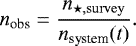 (C.1)
(C.1)Fixing n⋆,survey to 200 000 for Kepler, a population with nsystem(t) = 1000, would require 200 observers. Although all three populations simulate 1 000 systems, nsystem(t) may diminish with time. For the nominal populations, at 4 Gyr, NG74 has 998, NG75 has 999, and NG76 has 1 000 systems.
- 2.
The locations of the observers are distributed uniformly and homogeneously around the celestial sphere in the (X, Y, Z) coordinate system. This is done by generating two different random numbers u1, u2 ∈ [0, 1) and using inverse transform sampling to obtain polar coordinates:
 (C.2)
(C.2)This initial location of observers remains fixed for one NGPPS system. Spherical coordinates are converted to Cartesian giving v(X,Y,Z), the unit-normedvectorial location of an observer.
- 3.
To alignthe transit geometry, the Bern Model gives the position of a planet and its orbit in a different coordinate system, (x, y, z) with origin at the star. Here, x is along the periastron, (x, y) are in the orbital plane, and z points along the angular momentum vector of the planet. To proceed, the two coordinate systems must be aligned. This is done by rotating the initial location of all observers (given in X, Y, Z coordinates) with respect to each planet’s orbit (given in x, y, z coordinates) via three rotations (for details see Murray & Correia (2010))27:
 (C.3)
(C.3)Here,
 , and
, and  are the inverses of the standard SO(3) rotation matrices.
  aligns the line of nodes with the X-axis.
  aligns the reference plane with the orbital plane.
  rotates the reference plane such that the X-axis points along the periastron point of the orbit. The new location of the observer is given by the vector
  and in polar coordinates
  . In Fig. C.1 (left) an example of such rotation is shown.
Now the location of observers and the planetary orbits is known in the same coordinate system. This step ensures that the relative orientation between different planets is maintained, and information coming from all orbital elements is used.
- 4.
Next, we estimate the angular width of the TSB. The semi-cone angle ψ, subtended by the planet’s shadow as it blocks starlight at the azimuthal location of observer
 is given by (Winn 2010)
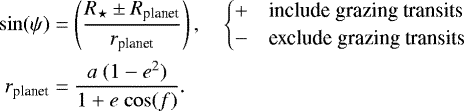 (C.4)
(C.4)Here, rplanet is the star–planet distance when the planet’s true anomaly is
 28. Finally, it is checked whether the observer
  is inside the TSB through the following condition:
![Mathematical equation: \begin{equation*} \begin{split} \alpha \in \left[\frac{\pi}{2} - \psi, \frac{\pi}{2} + \psi \right] &\rightarrow \text{Inside TSB}, \\ \text{otherwise} &\rightarrow \text{Outside TSB}. \end{split} \end{equation*}](/articles/aa/full_html/2021/12/aa40761-21/aa40761-21-eq42.png) (C.5)
(C.5)This information is now stored for a planet at the original location of the observer Oi (θ, ϕ).
- 5.
Repeat from step 4 for all nobs observers.
- 6.
Repeat from step 3 for all planets in a system.
- 7.
Repeat from step 2 for all systems in a population.
Figure C.1 (right) displays the result from KOBE-Shadows for a system with 24 planets in NG76. This calculation, done us- ing 106 observers and considering only full transits, takes about 1s.
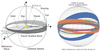 |
Fig. C.1 Thegeometry of transiting planets as implemented in KOBE. Left: Transit geometry for a single star–planet system. The dashed red arrow represents the initial location of an observer Oi(θ, ϕ), and the solidred arrow gives the rotated location of same observer Oi(f, α) (see text for details). Right: Example of transit shadow bands for a 24-planet system (star and planets are not shown). KOBE-Shadows calculates whether an observer is present inside the fulltransit shadow band of any planet in this system. The innermost planet has Ptra =12% and is detectable by observers marked in blue. The second (Ptra = 6%) and the third innermost planet (Ptra = 2%) are detectable by observers (in orange and green, respectively). The probability to potentially detect any four planets simultaneously via transit for this system is ~ 8%, which is halved for simultaneously detecting any nine planets. |
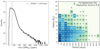 |
Fig. C.2 Inputs required by KOBE to simulate the Kepler transit survey. Left: Distribution of stellar noise, rms CDPP6 h, as seen by Kepler for FGK solar-type stars. Each individual KOBE system is assigned a CDPP value from this distribution. Right: Two-dimensional histogram depicting completeness of Kepler’s Robovetter, as calculated by KOBE-Vetter. To emulatehigh reliability, a disposition score cut-off is placed. Labels on each bin indicate the completeness (in %) for that bin. This calculation is based on the injected transit signals (Coughlin 2017). Completeness is not calculated for bins with less than ten injected signals (not labelled). These bins are assigned a completeness of 0%. |
These calculations undergo two major consistency checks. Firstly, the area under a planet’s TSB over the area of the celestial sphere gives the transit probability for this planet. Here, the number of observers found inside a TSB over nobs gives a numerical proxy for the same. The analytical expression for transit probability, Ptra, of a planet can be easily derived (Barnes 2007):
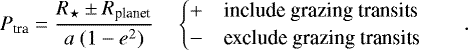 (C.6)
(C.6)
The numerical and analytical values of Ptra, with varying nobs from 105 to 108, are found to be in good agreement. In addition, the transit probability for multiple planets is available for free via the numerical recipe described above. Finding the same through analytical approaches is a difficult problem.
Secondly, the impact parameter of a transiting planet for all observers inside the TSB should be less than 1 + (Rplanet∕R⋆). The impact parameter, b, is the sky-projected star–planet distance expressed in units of stellar radii, and is given by
 (C.7)
(C.7)
The impact parameter for an observer  , is calculated by identifying i = α. This condition is satisfied by all observers that are inside the TSB, for all planets, for all systems, in all three populations.
The above procedure produces the KOBE-Shadows catalogue, which consists of KOBE systems containing at least one transiting planet. Although all of the planets in this catalogue will transit, not all of them will be detected. KOBE-Transits takes care of this problem.
C.2 KOBE-Transits
KOBE-Transits examines the transit signal for all transiting planets found by KOBE-Shadows. To be detected a transiting planet has to produce a signal that is strong enough to be de- tected by observers. To check this, KOBE-Transits calculates the transit S/N. An estimate of the noise as seen by an observer is required for this.
In KOBE-Transits noise for a KOBE System is sampled from the distribution of rms combined differential photometric precision (CDPP). Produced by the Kepler pipeline (DR25) for individual target stars, CDPP is an empirical measure of the stellar photometric noise (Christiansen et al. 2012)29. Three cuts are placed on this distribution to ensure that FGK solar-type stars are sampled. These are on mass M⋆ ∈ [0.7, 1.3]M⊙, on radius R⋆ ≤ 5 R⊙, and on stellar temperatureT⋆ ∈ [3880, 7200] K (Pecaut & Mamajek 2013).
The amount of stellar flux blocked by a planet is proportional to its area. The transit signal generated by a single transit is  . The single transit S/N is
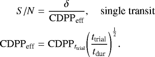 (C.8)
(C.8)
Here, CDPPeff is the effective stellar noise seen by an observer during a transit of duration tdur.  is the rms CDPP calculated by the Kepler pipeline for different trials of transit durations (varying from 1.5 h to 15 h). Following W18, here ttrial = 6 h. Figure C.2 (left) shows the distribution of rms CDPP6 h after placing the above cuts. To enhance the independent treatment of KOBE systems, a noise value is drawn randomly from the rms CDPP6 h distribution for every star in the KOBE-Shadows catalogue.
The transit duration for a planet is estimated by the time taken by a planet to cross the stellar disk. Following W18, circular orbits and b = 0 are assumed. This gives
 (C.9)
(C.9)
When a planet’s transit is observed ntra times, the multi-transit S/N improves by a factor of  . For a planet with period P and transit survey of duration tsurvey, the average number of transits can be estimated as ntra = tsurvey∕P. Then the multi-transit S/N generated by a transiting planet for tsurvey = tkepler = 3.5 yr is
![Mathematical equation: \begin{equation*}S/N = \underbrace{\bigg(\frac{R_{\textrm{planet}}}{R_{\star}}\bigg)^2}_{= \delta} \ \underbrace{\bigg(\frac{R_{\star}}{a}\bigg)^{\frac{1}{2}}}_{= P_{\textrm{tra}}} \ \bigg[ \bigg(\frac{t_{\textrm{kepler}}}{\pi \ t_{\textrm{trial}}}\bigg)^{\frac{1}{2}} \ \frac{1}{\mathrm{CDPP}_{t_{\textrm{trial}}}}\bigg]. \end{equation*}](/articles/aa/full_html/2021/12/aa40761-21/aa40761-21-eq51.png) (C.10)
(C.10)
This equation shows that the transit S∕N is given by the transit signal generated by a planet, multiplied by a factor  , scaled with instrument- and survey-related constants. Thus, a large planet closely orbiting a small quiet star will produce a high S∕N. These are some of the detection biases of the transit method.
In KOBE-Transits transiting planets that have S∕N ≥ 7.1 and ntra ≥ 2 constitute the KOBE-periodic threshold crossing event (pTCE) catalogue. For the Kepler pipeline, the threshold for detection of a TCE was multiple event statistic (MES, analogous to multi-transit S/N) ≥ 7.1σ, and ntra ≥ 3 (Twicken et al. 2016, 2018; Christiansen et al. 2012; Thompson et al. 2018). Following W18, the minimum ntra is fixed to 2.
C.3 KOBE-Vetter
In Thompson et al. (2018), the DR25 TCE are further reviewed by an automatic program, the Robovetter. The Robovetter examines several metrics, and identifies consistent TCEs as Kepler objects of interest (KOIs). Through further analysis, the Robovetter eventually vets KOIs as either planet candidates or false positives. However, not all candidates are true exoplanets and some false positives may have been genuine signals.
The catalogue produced by the Robovetter was characterized for completeness and reliability. Completeness measures the fraction of true planets that are absent in the catalogue, and reliability measures the fraction of planetary candidates that are truly exoplanets (Coughlin 2017). These measurements are done by injecting simulated transit signals in the Robovetter. The Robovetter completeness is given by the fraction of injected transit signals that are characterized as planetary candidates. The confidence of vetting a TCE as a planetary candidate is expressed with a disposition score (ranging from 0 to 1, a higher value implying higher confidence that a TCE is a candidate). Selecting only high scoring candidates produces a catalogue that has less completeness, but is highly reliable.30
KOBE-Vetter calculates the Robovetter completeness (for disposition score ≥ 0.9) using the results of these injection tests (Coughlin 2017)31. Completeness is calculated as a function of planetary radius (bin size 2 R⊕) and period (bin size 50 d). Figure C.2 (right) shows a 2D histogram of completeness (including reliability). These values are applied to the pTCE catalogue in a straightforward manner. If a 2D bin has completeness of C%, then for all planets in the pTCE catalogue that fall in this bin C% are randomly vetted as candidates and make the planetary candidates catalogue. The rest are rejected as false positives. For example, if there are 100 planets with Rplanet ∈ [0, 2)R⊕ and P ∈ [300, 350) d in the pTCE catalogue, then 33 planets will be randomly marked as candidates and the remaining 66 planets are vetted as false positives.
References
- Adams, F. C. 2019, MNRAS, 488, 1446 [NASA ADS] [CrossRef] [Google Scholar]
- Adams, F. C., Batygin, K., Bloch, A. M., & Laughlin, G. 2020, MNRAS, 493, 5520 [NASA ADS] [CrossRef] [Google Scholar]
- Alibert, Y. 2019, A&A, 624, A45 [NASA ADS] [CrossRef] [EDP Sciences] [Google Scholar]
- Alibert, Y., Mordasini, C., & Benz, W. 2004, A&A, 417, L25 [NASA ADS] [CrossRef] [EDP Sciences] [Google Scholar]
- Alibert, Y., Mordasini, C., Benz, W., & Winisdoerffer, C. 2005, A&A, 434, 343 [NASA ADS] [CrossRef] [EDP Sciences] [Google Scholar]
- Alibert, Y., Mordasini, C., & Benz, W. 2011, A&A, 526, A63 [NASA ADS] [CrossRef] [EDP Sciences] [Google Scholar]
- Alibert, Y., Carron, F., Fortier, A., et al. 2013, A&A, 558, A109 [NASA ADS] [CrossRef] [EDP Sciences] [Google Scholar]
- Armstrong, D. J., Lopez, T. A., Adibekyan, V., et al. 2020, Nature, 583, 39 [Google Scholar]
- Baillié, K., Marques, J., & Piau, L. 2019, A&A, 624, A93 [NASA ADS] [CrossRef] [EDP Sciences] [Google Scholar]
- Baraffe, I., Homeier, D., Allard, F., & Chabrier, G. 2015, A&A, 577, A42 [NASA ADS] [CrossRef] [EDP Sciences] [Google Scholar]
- Barnes, J. 2007, PASP, 119, 986 [NASA ADS] [CrossRef] [Google Scholar]
- Bashi, D., & Zucker, S. 2021, A&A, 651, A61 [NASA ADS] [CrossRef] [EDP Sciences] [Google Scholar]
- Benz, W., Ida, S., Alibert, Y., Lin, D., & Mordasini, C. 2014, in Protostars and Planets VI, eds. H. Beuther, R. Klessen, C. Dullemond, & T. Henning (Tucson: University of Arizona), 691 [Google Scholar]
- Borucki, W. J. 2016, Rep. Progr. Phys., 79, 036901 [Google Scholar]
- Borucki, W. J., & Summers, A. L. 1984, Icarus, 58, 121 [CrossRef] [Google Scholar]
- Borucki, W. J., Koch, D., Basri, G., et al. 2010, Science, 327, 977 [Google Scholar]
- Borucki, W. J., Koch, D. G., Basri, G., et al. 2011, ApJ, 736, 19 [Google Scholar]
- Brügger, N., Alibert, Y., Ataiee, S., & Benz, W. 2018, A&A, 619, A174 [Google Scholar]
- Brügger, N., Burn, R., Coleman, G. A. L., Alibert, Y., & Benz, W. 2020, A&A, 640, A21 [NASA ADS] [CrossRef] [EDP Sciences] [Google Scholar]
- Bryson, S., Coughlin, J., Batalha, N. M., et al. 2020, AJ, 159, 279 [NASA ADS] [CrossRef] [Google Scholar]
- Burrows, A., Hubeny, I., Budaj, J., & Hubbard, W. B. 2007, ApJ, 661, 502 [NASA ADS] [CrossRef] [Google Scholar]
- Chambers, J. E. 1999, MNRAS, 304, 793 [Google Scholar]
- Chambers, J., Wetherill, G., & Boss, A. 1996, Icarus, 119, 261 [NASA ADS] [CrossRef] [Google Scholar]
- Chevance, M., Kruijssen, J. M. D., & Longmore, S. N. 2021, ApJ, 910, L19 [NASA ADS] [CrossRef] [Google Scholar]
- Christiansen, J. L., Jenkins, J. M., Barclay, T. S., et al. 2012, PASP, 124, 1279 [NASA ADS] [CrossRef] [Google Scholar]
- Ciardi, D. R., Fabrycky, D. C., Ford, E. B., et al. 2013, ApJ, 763, 41 [CrossRef] [Google Scholar]
- Clarke, C. J., Gendrin, A., & Sotomayor, M. 2001, MNRAS, 328, 485 [NASA ADS] [CrossRef] [Google Scholar]
- Coleman, G. A., & Nelson, R. P. 2014, MNRAS, 445, 479 [NASA ADS] [CrossRef] [Google Scholar]
- Coughlin, J. L. 2017, KSCI-19 114-001, 1 [Google Scholar]
- Deck, K. M., Payne, M., & Holman, M. J. 2013, ApJ, 774, 129 [Google Scholar]
- Demory, B. O., Gillon, M., De Wit, J., et al. 2016, Nature, 532, 207 [NASA ADS] [CrossRef] [Google Scholar]
- Dittkrist, K. M., Mordasini, C., Klahr, H., Alibert, Y., & Henning, T. 2014, A&A, 567, A121 [NASA ADS] [CrossRef] [EDP Sciences] [Google Scholar]
- Emsenhuber, A., Mordasini, C., Burn, R., et al. 2021a, A&A, 656, A69 (Paper I) [NASA ADS] [CrossRef] [EDP Sciences] [Google Scholar]
- Emsenhuber, A., Mordasini, C., Burn, R., et al. 2021b, A&A, 656, A70 (Paper II) [NASA ADS] [CrossRef] [EDP Sciences] [Google Scholar]
- Espinoza, N., Brahm, R., Henning, T., et al. 2020, MNRAS, 491, 2982 [NASA ADS] [Google Scholar]
- Evans, T. M., Sing, D. K., Wakeford, H. R., et al. 2016, ApJ, 822, L4 [NASA ADS] [CrossRef] [Google Scholar]
- Fabrycky, D. C., Lissauer, J. J., Ragozzine, D., et al. 2014, ApJ, 790, 146 [Google Scholar]
- Flaherty, K., Hughes, A. M., Simon, J. B., et al. 2020, ApJ, 895, 109 [NASA ADS] [CrossRef] [Google Scholar]
- Fortier, A., Alibert, Y., Carron, F., Benz, W., & Dittkrist, K.-M. 2013, A&A, 549, A44 [NASA ADS] [CrossRef] [EDP Sciences] [Google Scholar]
- Fulton, B. J., Petigura, E. A., Howard, A. W., et al. 2017, AJ, 154, 109 [Google Scholar]
- Gilbert, G. J., & Fabrycky, D. C. 2020, AJ, 159, 281 [Google Scholar]
- Guillot, T. 2010, A&A, 520, A27 [NASA ADS] [CrossRef] [EDP Sciences] [Google Scholar]
- Hadden, S., & Lithwick, Y. 2017, AJ, 154, 5 [Google Scholar]
- He, M. Y., Ford, E. B., & Ragozzine, D. 2019, MNRAS, 490, 4575 [CrossRef] [Google Scholar]
- Heng, K. 2019, MNRAS, 490, 3378 [NASA ADS] [CrossRef] [Google Scholar]
- Hoeijmakers, H. J., Ehrenreich, D., Heng, K., et al. 2018, Nature, 560, 453 [CrossRef] [Google Scholar]
- Hsu, D. C., Ford, E. B., Ragozzine, D., & Morehead, R. C. 2018, AJ, 155, 205 [NASA ADS] [CrossRef] [Google Scholar]
- Hueso, R., & Guillot, T. 2005, A&A, 442, 703 [NASA ADS] [CrossRef] [EDP Sciences] [Google Scholar]
- Hunter, J. D. 2007, Comput. Sci. Eng., 9, 90 [NASA ADS] [CrossRef] [Google Scholar]
- Ida, S., & Lin, D. N. C. 2004, ApJ, 616, 567 [NASA ADS] [CrossRef] [Google Scholar]
- Jin, S., Mordasini, C., Parmentier, V., et al. 2014, ApJ, 795, 65 [Google Scholar]
- Johansen, A., Oishi, J. S., Low, M. M. M., et al. 2007, Nature, 448, 1022 [NASA ADS] [CrossRef] [Google Scholar]
- Johnson, J. A., Petigura, E. A., Fulton, B. J., et al. 2017, AJ, 154, 108 [Google Scholar]
- King, A. 2009, A&A, 500, 53 [NASA ADS] [CrossRef] [EDP Sciences] [Google Scholar]
- Kipping, D. 2018, MNRAS, 473, 784 [NASA ADS] [CrossRef] [Google Scholar]
- Kipping, D. M., & Sandford, E. 2016, MNRAS, 463, 1323 [NASA ADS] [CrossRef] [Google Scholar]
- Kley, W., & Dirksen, G. 2006, A&A, 447, 369 [NASA ADS] [CrossRef] [EDP Sciences] [Google Scholar]
- Kokubo, E., & Ida, S. 1998, Icarus, 131, 171 [Google Scholar]
- Kokubo, E., & Ida, S. 2002, ApJ, 581, 666 [Google Scholar]
- Kreidberg, L., Bean, J. L., Désert, J. M., et al. 2014, Nature, 505, 69 [NASA ADS] [CrossRef] [Google Scholar]
- Leleu, A., Coleman, G. A. L., & Ataiee, S. 2019, A&A, 631, A6 [NASA ADS] [CrossRef] [EDP Sciences] [Google Scholar]
- Lissauer, J. J., Ragozzine, D., Fabrycky, D. C., et al. 2011, ApJS, 197, 8 [Google Scholar]
- Lodders, K. 2003, ApJ, 591, 1220 [Google Scholar]
- Lüst, R. 1952, Z. Naturforsch. Teil A, 7, 87 [CrossRef] [Google Scholar]
- Lynden-Bell, D., & Pringle, J. E. 1974, MNRAS, 168, 603 [Google Scholar]
- MacDonald, M. G., Dawson, R. I., Morrison, S. J., Lee, E. J., & Khandelwal, A. 2020, ApJ, 891, 20 [NASA ADS] [CrossRef] [Google Scholar]
- Manara, C. F., Mordasini, C., Testi, L., et al. 2019, A&A, 631, L2 [NASA ADS] [CrossRef] [EDP Sciences] [Google Scholar]
- Marboeuf, U., Thiabaud, A., Alibert, Y., Cabral, N., & Benz, W. 2014, A&A, 570, A35 [Google Scholar]
- Matsuyama, I., Johnstone, D., & Murray, N. 2003, ApJ, 585, L143 [NASA ADS] [CrossRef] [Google Scholar]
- Mayor, M., & Queloz, D. 1995, Nature, 378, 355 [Google Scholar]
- Mayor, M., Marmier, M., Lovis, C., et al. 2011, ArXiv e-prints [arXiv:1109.2497] [Google Scholar]
- Millholland, S., Wang, S., & Laughlin, G. 2017, ApJ, 849, L33 [NASA ADS] [CrossRef] [Google Scholar]
- Mishra, L., Alibert, Y., & Udry, S. 2019, in EPSC-DPS Joint Meeting 2019, 2019, EPSC–DPS2019–1616 [Google Scholar]
- Mordasini, C. 2018, Planetary Population Synthesis, eds. H. J. Deeg, & J. A. Belmonte, 143 [Google Scholar]
- Mordasini, C., Alibert, Y., Benz, W., Klahr, H., & Henning, T. 2008, PhD thesis [Google Scholar]
- Mordasini, C., Alibert, Y., Benz, W., & Naef, D. 2009, A&A, 501, 1161 [NASA ADS] [CrossRef] [EDP Sciences] [Google Scholar]
- Mordasini, C., Alibert, Y., Benz, W., Klahr, H., & Henning, T. 2012a, A&A, 541, A97 [NASA ADS] [CrossRef] [EDP Sciences] [Google Scholar]
- Mordasini, C., Alibert, Y., Georgy, C., et al. 2012b, A&A, 547, A112 [NASA ADS] [CrossRef] [EDP Sciences] [Google Scholar]
- Mordasini, C., Alibert, Y., Klahr, H., & Henning, T. 2012c, A&A, 547, A111 [NASA ADS] [CrossRef] [EDP Sciences] [Google Scholar]
- Mordasini, C., Mollière, P., Dittkrist, K.-M., Jin, S., & Alibert, Y. 2015, Int. J. Astrobiol., 14, 201 [NASA ADS] [CrossRef] [Google Scholar]
- Mordasini, C., Marleau, G. D., & Mollière, P. 2017, A&A, 608, A72 [NASA ADS] [CrossRef] [EDP Sciences] [Google Scholar]
- Mulders, G. D., Pascucci, I., Apai, D., & Ciesla, F. J. 2018, AJ, 156, 24 [Google Scholar]
- Mulders, G. D., Mordasini, C., Pascucci, I., et al. 2019, ApJ, 887, 157 [NASA ADS] [CrossRef] [Google Scholar]
- Mulders, G. D., O’brien, D. P., Ciesla, F. J., Apai, D., & Pascucci, I. 2020, ApJ, 897, 72 [NASA ADS] [CrossRef] [Google Scholar]
- Murchikova, L., & Tremaine, S. 2020, AJ, 160, 160 [NASA ADS] [CrossRef] [Google Scholar]
- Murray, C. D., & Correia, A. C. M. 2010, Keplerian Orbits and Dynamics of Exoplanets, ed. S. Seager, 15 [Google Scholar]
- Nakamoto, T.,& Nakagawa, Y. 1994, ApJ, 421, 640 [NASA ADS] [CrossRef] [Google Scholar]
- Oliphant, T. E. 2006, A guide to NumPy, 1 (Trelgol Publishing USA) [Google Scholar]
- Paardekooper,S. J., Baruteau, C., & Kley, W. 2011, MNRAS, 410, 293 [NASA ADS] [CrossRef] [Google Scholar]
- pandas development team, T. 2020, pandas-dev/pandas: Pandas [Google Scholar]
- Pecaut, M. J.,& Mamajek, E. E. 2013, ApJS, 208, 9 [Google Scholar]
- Petigura, E. A., Howard, A. W., Marcy, G. W., et al. 2017, AJ, 154, 107 [NASA ADS] [CrossRef] [Google Scholar]
- Pollack, J. B., Hubickyj, O., Bodenheimer, P., et al. 1996, Icarus, 124, 62 [NASA ADS] [CrossRef] [Google Scholar]
- Rauer, H., Catala, C., Aerts, C., et al. 2014, Exp. Astron., 38, 249 [Google Scholar]
- Ricker, G. R., Winn, J. N., Vanderspek, R., et al. 2014, J. Astron. Telescopes, Instrum. Syst., 1, 014003 [NASA ADS] [CrossRef] [Google Scholar]
- Sandford, E., Kipping, D., & Collins, M. 2019, MNRAS, 489, 3162 [Google Scholar]
- Santerne, A., Malavolta, L., Kosiarek, M. R., et al. 2019, ArXiv e-prints [arXiv:1911.07355] [Google Scholar]
- Santos, N. C., Israelian, G., Mayor, M., et al. 2005, A&A, 437, 1127 [NASA ADS] [CrossRef] [EDP Sciences] [Google Scholar]
- Sarkis, P., Mordasini, C., Henning, T., Marleau, G. D., & Mollière, P. 2021, A&A, 645, A79 [NASA ADS] [CrossRef] [EDP Sciences] [Google Scholar]
- Schneider, J., Dedieu, C., Le Sidaner, P., Savalle, R., & Zolotukhin, I. 2011, A&A, 532, A79 [NASA ADS] [CrossRef] [EDP Sciences] [Google Scholar]
- Shakura, N. I., & Sunyaev, R. A. 1973, A&A, 24, 337 [NASA ADS] [Google Scholar]
- Sing, D. K., Fortney, J. J., Nikolov, N., et al. 2016, Nature, 529, 59 [Google Scholar]
- Thiabaud, A., Marboeuf, U., Alibert, Y., et al. 2014, A&A, 562, A27 [NASA ADS] [CrossRef] [EDP Sciences] [Google Scholar]
- Thompson, S. E., Coughlin, J. L., Hoffman, K., et al. 2018, ApJS, 235, 38 [NASA ADS] [CrossRef] [Google Scholar]
- Twicken, J. D., Jenkins, J. M., Seader, S. E., et al. 2016, AJ, 152, 158 [NASA ADS] [CrossRef] [Google Scholar]
- Twicken, J. D., Catanzarite, J. H., Clarke, B. D., et al. 2018, PASP, 130, 064502 [Google Scholar]
- Tychoniec, Ł., Tobin, J. J., Karska, A., et al. 2018, ApJS, 238, 19 [Google Scholar]
- Udry, S., & Santos, N. C. 2007, ARA&A, 45, 397 [NASA ADS] [CrossRef] [Google Scholar]
- Van Rossum, G., & Drake, F. L. 2009, Python 3 Reference Manual (Scotts Valley, CA: CreateSpace) [Google Scholar]
- Venturini, J., Guilera, O. M., Haldemann, J., Ronco, M. P., & Mordasini, C. 2020, A&A, 643, L1 [NASA ADS] [CrossRef] [EDP Sciences] [Google Scholar]
- Venuti, L., Bouvier, J., Cody, A. M., et al. 2017, A&A, 599, A23 [NASA ADS] [CrossRef] [EDP Sciences] [Google Scholar]
- Veras, D., & Armitage, P. J. 2004, MNRAS, 347, 613 [Google Scholar]
- Virtanen, P., Gommers, R., Oliphant, T. E., et al. 2020, Nat. Methods, 17, 261 [Google Scholar]
- Wang, S. 2017, Res. Notes Am. Astron. Soc., 1, 26 [Google Scholar]
- Waskom, M. & the seaborn development team 2020, mwaskom/seaborn [Google Scholar]
- Weiss, L. M., & Petigura, E. A. 2020, ApJ, 893, L1 [Google Scholar]
- Weiss, L. M., Marcy, G. W., Petigura, E. A., et al. 2018, AJ, 155, 48 [Google Scholar]
- Williams, J. P., & Cieza, L. A. 2011, ARA&A, 49, 67 [Google Scholar]
- Winn, J. N. 2010, ArXiv e-prints [arXiv:1001.2010] [Google Scholar]
- Winn, J. N., & Fabrycky, D. C. 2015, ARA&A, 53, 409 [Google Scholar]
- Winn, J. N., Sanchis-Ojeda, R., & Rappaport, S. 2018, New Astron. Rev., 83, 37 [CrossRef] [Google Scholar]
- Xu, W., Lai, D., & Morbidelli, A. 2018, MNRAS, 481, 1538 [Google Scholar]
- Youdin, A. 2008, in EAS Publications Series, ed. T. Montmerle, D. Ehrenreich, & A. M. Lagrange (EAS Publications Series) [Google Scholar]
- Zar, J. H. 2014, Biostatistical Analysis, 5th edn. (Essex: Pearson), 761 [Google Scholar]
- Zhu, W. 2020, AJ, 159, 188 [NASA ADS] [CrossRef] [Google Scholar]
Based on a September 2020 query of the Extrasolar Planets Encyclopaedia (Schneider et al. 2011).
Lowercase r is used for radial distance of an object (e.g. distance from the star), while capital R is used to denote the radius of the object itself.
Alternative definitions of entropy are also explored by incorporating a memory-like term to include size ordering from one adjacent pair of planets to the next adjacent pair of planets.
For example, Sandford et al. (2019) estimate that around ≃2400 more exoplanets reside in 1537 planet hosting FGK stars observed by Kepler.
Zhu (2020) point out that resampling transit S/N is a ‘shortcut’ for a ‘more appropriate way’. This appropriate way includes an intrinsic planetary distribution with a full-forward model of the transit detection bias. In this paper the Bern Model provides an intrinsic, albeit synthetic, population of exoplanets, and KOBE models the Kepler transit survey.
A set of hundreds or thousands of individual planetary systems are referred to here as a population.
Readers who are well versed with the Bern Model and its updates may skip to Sect. 4 where KOBE is introduced. Other readers may use this introductory section as a starting point for key concepts and relevant literature for planet formation in general, and the Bern Model in particular.
A global model, which comprises of theoretical models for individual physical processes linked together coherently, calculates the final planetary system based on a set of initial conditions.
The number of simulated systems (1000) is chosen to be of the same order of magnitude as observed exoplanetary systems: 355 in CKSM (W18), 822 in HARPS-GTO (Mayor et al. 2011), and ~3000 overall (Schneider et al. 2011).
In an alternative approach, some of the solid disk mass could be partitioned into pebbles. For a comparison of planet formation via pebble accretion and planetesimal accretion, see Brügger et al. (2018, 2020).
Due to their small size, these objects are virtually undetectable via the transit method and do not affect the results of this paper.
The current version of KOBE is designed to simulate NASA’s Kepler space telescope. However, KOBE is not limited to the Kepler survey and can be easily tweaked to simulate other transit surveys like TESS and PLATO (Ricker et al. 2014; Rauer et al. 2014).
Following W18, the minimum number of transits is fixed at two.
In addition to the Pearson R correlation test, the Spearman R correlation test was also performed for all correlations. The Spearman R tests for correlations (specifically monotonicity) in the rank of members of two datasets instead of their actual value.
Following W18, the size correlation coefficient Pearson R is calculated on the log of radius. Since the Spearman R is calculated on the rank of the members in a dataset, taking a log produces no difference in the coefficient’s value.
The Spearman correlation coefficient is unity (R = 1) for a strictly monotonic function.
See Zhu (2020) and Weiss & Petigura (2020) for a discussion and justification of this choice.
An ordered pair is one in which the outer planet (from the star) has the larger value for a given quantity (e.g. radius, mass).
Each stage of KOBE’s calculation introduces some randomness (location of observers or vetting planetary candidates). Even if all planets in a system were in the same orbital planet, the randomness inherent in KOBE’s calculation or the variation in their sizes could lead to random missing planets.
Oligarchic embryos offer only a partial explanation of the early mass–size similarity. In other words, oligarchic embryos do not explain why adjacent planets have similar masses on Myr timescales. To check this, a 50-embryo population was simulated where the embryos had initial masses between 0.0001M⊕ and 0.01M⊕. We find that this synthetic population shows similar (but slightly weaker) mass similarity correlations as the population with fixed initial embryo mass (at early and late times). In addition, the final mass of a planet seems to have little dependence on the initial embryo mass. If fixed initial embryo mass could explain mass similarity on Myr timescales, then we would have seen weak or no mass similarity correlation in the population where embryo masses were varied, which does not seem to be the case here. This indicates that additional physics involved in planet formation is essential for obtaining a detailed understanding of the peas in a pod mass similarity trend.
Following Paper II, giant planets are defined as planets with Mplanet >= 300 M⊕.
α measures efficiency of transport due to turbulence. Since random isotropic motions do not have length scales larger than the local disk scale height, α is usually < 1 (King 2009).
In the first ~105 years the disk gains mass from the molecular cloud collapse. This can be modelled by adding a source term to eq. B.1, as is done in Hueso & Guillot (2005).
This is because (a) the disk is geometrically thin and (b) the disk is assumed to be optically thick along the radial direction.
KOBE systems, being subsets of the NGPPS systems, are not truly independent. In KOBE a single observer observing 1000 synthetic planetary systems may detect ~ 100 transiting planets around ~ 50 stars. The strategy of using multiple observers in KOBE grew out of a need to (a) find more transiting planets, (b) imprint the effect of transit probability (via TSB calculation), and (c) systematize KOBE’s approach.
A planet’s position on the orbit,  , is not required to calculate its TSB because the calculation is done for virtually all positions on the orbit.
Equivalently, the planet’s orbit could be rotated, keeping the location of observers fixed.
For this paper, grazing transits are excluded.
This data is available in tabular format from the NASA Exoplanet Archive.
Thompson et al. (2018) suggested using a cut on disposition score for occurrence rate studies. This approach has been used by Mulders et al. (2018) and Hsu et al. (2018), and extensively studied by Bryson et al. (2020).
The Robovetter Disposition Table is available from the NASA Exoplanet Archive.
All Figures
|
Fig. 1 Bern Model: schematic diagram (not drawn to scale) illustrating the breadth of physical processes incorporated in the Generation III Bern Model of Planet Formation and Evolution. Panels a and b show the fixed and varying initial conditions, respectively. The physical processes relevant to the protoplanetary disk are indicated in panel c. It represents a snapshot of the starting point of the model: several protoplanetary embryos are embedded in a disk of gas and planetesimals. The processes that govern planet formation and evolution are displayed in panel d. In panel e, additional physics incorporated in the model is shown. The arrows indicate the evolution of a fixed mass star. Most of the depicted physical processes occur simultaneously and not all processes are shown. See text for summary and Paper I for details. |
| In the text | |
|
Fig. 2 Effect of KOBE: Normalized cumulative distributions for radius (left) and period (right) for the 100 embryo population. The solid red curve represents the underlying population as calculated by the Bern Model. The orange curve is the output of KOBE-Shadows. KOBE-Transits’s pTCE catalogue is shown in light-blue, and the catalogue of planetary candidates, as vetted by KOBE-Vetter is shown in blue. |
| In the text | |
|
Fig. 3 Comparison of planetary populations. Theoretical (blue) represents planets in KOBE multi-planetary systems (KMPS) and observations (green) are the CKS multi-planetary systems (CKSM). Left: Scatter plot with planetary radius on the y-axis and period on the x-axis. The dashed line shows the maximum period of a planet that can be found by KOBE. The dotted line shows the minimum radius of a planet around a 1 R⊙ star for producing a transit S/N of 10. The underlying theoretical population is shown in grey. Right: Comparison of radius (top)and period (bottom) distributions. The radius valley can be clearly seen in the planets found by KOBE and the California-Kepler survey. |
| In the text | |
|
Fig. 4 Distribution of planetary multiplicity: Bern Model in grey, Bern Model detectable planets (P < 640 days) in black, KMPS in blue, and observed CKSM in green. The solid black line indicates the maximum number of TCE searches for a star performed by the Kepler pipeline. |
| In the text | |
|
Fig. 5 Peas in a pod. Comparison of the correlations present in the theoretically observed KMPS catalogue (theory) and the CKSM catalogue (observations). Also shown are the correlations present in the underlying Bern Model population (grey). |
| In the text | |
|
Fig. 6 Peas in a pod: size. The sizes of adjacent planets are shown for the underlying population (left), for the underlying population of detectable planets (P < 640 days) (middle), and for theoretical observed planets (right). |
| In the text | |
|
Fig. 7 Peas in a pod: mass. The masses of adjacent planets are shown for the underlying population (left), for the underlying population of detectable planets (P < 640 days) (middle), and for theoretical observed planets (right). |
| In the text | |
|
Fig. 8 Mass–radius relationship. Planetary radii are plotted as a function of planetary masses for the planets in the KMPS 100-embryo population. For planets with non-zero H–He envelopes, the colour denotes their envelope mass fraction,
|
| In the text | |
|
Fig. 9 Peas in a pod: spacing. The plots shows the period ratio of the outer pair of planets as a function of the period ratio of the inner pair for the underlying population (left), for the underlying population of detectable planets (middle), and for the KMPS systems (right). The dashed horizontal lines mark some of the important commensurabilities. The number inside the parenthesis is the percentage of outer planetary pairs that have a period ratio within 1% of the indicated commensurability. |
| In the text | |
|
Fig. 10 Peas in a pod: packing. The average sizes (top) and average masses (bottom) of adjacent planets are shown as a function of their orbital period ratios Pj+1 ∕Pj for the underlying population (left), underlying population of detectable planets (middle), and KMPS planets (right). For the underlying population, the position of the inner planet in each pair is in a different colour, showing that the trend is due to those planetary pairs where the inner planet is close to the host star. The black curveshows the Hill stability criterion from Deck et al. (2013). Adjacent planetary pairs on the right side of this curve are Hill stable. Points on the left side are Hill unstable and will probably be removed with longer N-body calculations. |
| In the text | |
|
Fig. 11 Influence of the geometrical limitations of the transit method (KOBE-Shadows), the transit detection biases (KOBE-Transits), and the completeness of the Kepler survey (KOBE-Vetter) on the peas in a pod trend. The plot shows how the correlation coefficients (left) and the frequency of ordered pairs (right) varies in the underlying Bern Model population, the underlying population of detectable planets (P < 640 days), and the theoretically observed KMPS population (for the size–mass trends in the KMPS catalogue adjacent planetary pairs have undergone a swapping test, as mentioned in Sect. 6.1). Observations from the CKSM exoplanetary catalogue are shown in green. |
| In the text | |
|
Fig. 12 Evolution of the peas in a pod trends. The vertical solid line represents the end of N-body calculations. |
| In the text | |
|
Fig. 13 Role of dynamical interactions on the peas in a pod trends. Left: distribution of lost planets [%] by systems in the 20-, 50-, and 100-embryo NGPPS populations. The fraction of planets lost by a system can be used as a proxy for the cumulative dynamical interactions experienced by a system. The dashed lines show the ratio of giant planets per system averaged over bins. Right: correlation coefficient for the peas in a pod trends for each bin. The error bars correspond to the standard error of the correlation coefficient (Zar 2014). Increasing dynamical interactions results in the strengthening of the spacing and packing trend. |
| In the text | |
|
Fig. A.1 Dependence of mutual separation of adjacent planets on their average sizes (top) and average masses (bottom). Observed exoplanetary populations (CKSM by W18) show a negative correlation between average sizes and mutual separation of adjacent planets, which is well reproduced here (top left). However, this negative correlation arises from the dependence of mutual Hill radii on the
1∕3 power of planetary masses. This is shown by the dashed line in the plots on the right. The vertical line marks the Hill stability criterion from Chambers et al. (1996). Points on the right side of this line are Hill stable ( |
| In the text | |
|
Fig. C.1 Thegeometry of transiting planets as implemented in KOBE. Left: Transit geometry for a single star–planet system. The dashed red arrow represents the initial location of an observer Oi(θ, ϕ), and the solidred arrow gives the rotated location of same observer Oi(f, α) (see text for details). Right: Example of transit shadow bands for a 24-planet system (star and planets are not shown). KOBE-Shadows calculates whether an observer is present inside the fulltransit shadow band of any planet in this system. The innermost planet has Ptra =12% and is detectable by observers marked in blue. The second (Ptra = 6%) and the third innermost planet (Ptra = 2%) are detectable by observers (in orange and green, respectively). The probability to potentially detect any four planets simultaneously via transit for this system is ~ 8%, which is halved for simultaneously detecting any nine planets. |
| In the text | |
|
Fig. C.2 Inputs required by KOBE to simulate the Kepler transit survey. Left: Distribution of stellar noise, rms CDPP6 h, as seen by Kepler for FGK solar-type stars. Each individual KOBE system is assigned a CDPP value from this distribution. Right: Two-dimensional histogram depicting completeness of Kepler’s Robovetter, as calculated by KOBE-Vetter. To emulatehigh reliability, a disposition score cut-off is placed. Labels on each bin indicate the completeness (in %) for that bin. This calculation is based on the injected transit signals (Coughlin 2017). Completeness is not calculated for bins with less than ten injected signals (not labelled). These bins are assigned a completeness of 0%. |
| In the text | |
Current usage metrics show cumulative count of Article Views (full-text article views including HTML views, PDF and ePub downloads, according to the available data) and Abstracts Views on Vision4Press platform.
Data correspond to usage on the plateform after 2015. The current usage metrics is available 48-96 hours after online publication and is updated daily on week days.
Initial download of the metrics may take a while.