| Issue |
A&A
Volume 692, December 2024
|
|
|---|---|---|
| Article Number | A122 | |
| Number of page(s) | 15 | |
| Section | Planets, planetary systems, and small bodies | |
| DOI | https://doi.org/10.1051/0004-6361/202451353 | |
| Published online | 06 December 2024 | |
Diversities and similarities exhibited by multi-planetary systems and their architectures
I. Orbital spacings
1
Department of Space, Earth and Environment, Chalmers University of Technology,
Chalmersplatsen 4,
412 58
Gothenburg,
Sweden
2
Department of Space, Earth and Environment, Chalmers University of Technology,
Onsala Space Observatory,
439 92
Onsala,
Sweden
3
Leiden Observatory, University of Leiden,
PO Box 9513,
2300 RA,
Leiden,
The Netherlands
★ Corresponding author; This email address is being protected from spambots. You need JavaScript enabled to view it.
Received:
2
July
2024
Accepted:
27
October
2024
Abstract
The rich diversity of multi-planetary systems and their architectures is greatly contrasted by the uniformity exhibited within many of these systems. Previous studies have shown that compact Kepler systems tend to exhibit a peas-in-a-pod architecture: Planets in the same system tend to have similar sizes and masses and be regularly spaced in orbits with low eccentricities and small mutual inclinations. This work extends on previous research and examines a larger and more diverse sample comprising all the systems with a minimum of three confirmed planets, resulting in 282 systems and a total of 991 planets. We investigated the system architectures, focusing on the orbital spacings between adjacent planets as well as their relationships with the planets’ sizes and masses. We also quantified the similarities of the sizes, masses, and spacings of planets within each system, conducting both intra- and inter-system analyses. Our results corroborate previous research showing that planets orbiting the same star tend to be regularly spaced and that pairs of adjacent planets with radii < 1 R⊕ predominantly have orbital period ratios (PRs) smaller than two. In contrast to other studies, we identified a significant similarity of adjacent orbital spacings not only at PRs < 4 but also at 1.17 < PRs < 2662. For the systems with transiting planets, we additionally found that the reported correlation between the orbital PRs and the average sizes of adjacent planets disappears when planet pairs with R < 1 R⊕ are excluded. Furthermore, we examined the data for possible correlations between the intra-system dispersions of the orbital spacings and those of the planetary radii and masses. Our findings indicate that these dispersions are uncorrelated for the systems in which all the pairs of adjacent planets have PRs < 6, and even for the compact systems where all PRs < 2. Notably, planets in the same system can be similarly spaced even if they do not have similar masses or sizes.
Key words: planets and satellites: detection / planets and satellites: fundamental parameters / planets and satellites: general
© The Authors 2024
 Open Access article, published by EDP Sciences, under the terms of the Creative Commons Attribution License (https://creativecommons.org/licenses/by/4.0), which permits unrestricted use, distribution, and reproduction in any medium, provided the original work is properly cited.
This article is published in open access under the Subscribe to Open model. This email address is being protected from spambots. You need JavaScript enabled to view it. to support open access publication.
1 Introduction
Over the past 30 years, our knowledge and achievements in exoplanetary science have increased at an accelerated rate. Technological advancements have empowered scientists to detect, characterise, and simulate an extraordinary plethora of both single- and multiple-planet systems. Surprisingly, many of these systems have astonishing yet unusual properties compared to the Solar System. Exceptionally, the Kepler space mission (Borucki et al. 2010) has revolutionised astronomy and led to the discovery of 3321 out of all the 5747 confirmed exoplanets to date1. This has enabled population-level planetary characterisations (e.g. Howard et al. 2012; Mulders 2018; Otegi et al. 2020) and statistics (Petigura et al. 2013; Zhu & Dong 2021; Hsu et al. 2019). Completely new and, at the same time, the most prevalent types of exoplanets are super-Earths (substantially rocky planets with radii 1.1 R⊕ ≲ R ≲ 1.8 R⊕) and sub-Neptunes (mainly gas and ice planets with radii 1.8 R⊕ ≲ R ≲ 3.5 R⊕). They are frequently found in compact multi-planetary systems at orbital periods ranging from mere hours to several months (Lissauer et al. 2011, 2014; Fabrycky et al. 2014; Winn & Fabrycky 2015).
The remarkable myriad of planets detected thus far provides us with the opportunity to study the variety of planet and system properties. The architecture of a system describes how the planets are arranged within the system and how their orbital and physical parameters are distributed. In addition, a system’s architecture could also provide valuable insights into the multitude of processes that have shaped the system. This may, thereby, enable improvement of the current models of planet formation and evolution.
The rich diversity of all the observed exoplanets and planetary systems is greatly contrasted by the uniformity exhibited within many of the multi-planetary systems (i.e. intra-system uniformity). Planets in the same system tend to have equal sizes and masses (e.g. Weiss et al. 2018b, 2023; Millholland et al. 2017) and be regularly spaced (e.g. Weiss et al. 2018b, 2023; Jiang et al. 2020) in orbits with low eccentricities (Van Eylen & Albrecht 2015; Xie et al. 2016; Hadden & Lithwick 2017) and small mutual inclinations (Fang & Margot 2012; Fabrycky et al. 2014). Hence, they are often similar to each other, resembling peas in a pod (Weiss et al. 2018b).
It was first reported by Lissauer et al. (2011) that pairs of adjacent planet candidates in Kepler systems tend to possess similar radii. Weiss et al. (2018b) corroborated this finding by examining multi-planetary systems (each harbouring at least two planet candidates) from the California-Kepler Survey (CKS) sample (Johnson et al. 2017, CKS II; see also Petigura et al. 2017, CKS I). They also reported that in systems with a minimum of three planets, the orbital spacing between two adjacent planets, in terms of their period ratio (PR), tends to be similar to the period ratio of the next pair of adjacent planets for PRs < 4. Furthermore, they identified a positive correlation between the PRs and the radii of adjacent planets. In particular, small-sized planet pairs with radii of R < 1 R⊕ were found to possess typical orbital period ratios < 2. The intra-system similarity in planetary radii and orbital spacings has been shown to encompass the planetary masses as well (Millholland et al. 2017; Wang 2017).
This paper is the first in a series focusing on the diversities and similarities exhibited between multi-planetary systems (inter-system) as well as within each system. In the work presented here, we investigate the architectures of observed multi-planetary systems with respect to the orbital spacings (period ratios) of adjacent planets as well as their relationships with the planets’ sizes and masses. We explore the similarities and differences of the orbital spacings both on a system level (in each system individually) as well as on a population level. The latter comprises: i) analysing together all the pairs of adjacent planets from all the systems and ii) conducting intersystem comparisons based on the spacing architecture of each system.
Previous studies on orbital spacings in observed planetary systems have only focused on systems with transiting planets and candidates detected by Kepler (e.g. Weiss et al. 2018b, 2023; Jiang et al. 2020). In contrast to these, we examine a much larger sample and only include confirmed planets in order to improve the reliability of the data. Our largest data catalogue comprises all systems with at least three planets, thereby encompassing multiple observation techniques: transit photometry, radial velocities (RVs), transit timing variations (TTVs), and direct imaging. This work analyses a much wider range of planetary systems, including orbital periods up to 170 000 days and period ratios up to 2662.
The key aspects explored in this work are as follows: (i) We study whether the spacing similarity trend holds true for our larger and more heterogeneous data sample, for instance, for systems with non-transiting or larger planets. (ii) We also investigate which system- or population-level relationships between orbital spacings and planetary sizes or masses emerge in our sample.
We organised this paper as follows: The data catalogues as well as the distributions of orbital periods and planet radii are presented in Sect. 2. We examine the orbital period ratios both on a population and system level in Sect. 3. The relationships between the orbital spacings and the planetary radii and masses are investigated in Sects. 4 and 5, respectively. The orbital separations in units of mutual Hill radii are explored in Sect. 6. We discuss our main results, including possible effects of observational biases, in Sect. 7 and end with conclusions in Sect. 8.
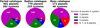 |
Fig. 1 Distribution of all the 282, 225, and 46 multi-planetary systems in the period, radius, and mass catalogue, respectively. In white is written the number of systems with any of the four observed planet multiplicities: systems with three (magenta); four (green), five (blue), and either six, seven, or eight (red) planets. Each of these systems has minimum three confirmed planets orbiting a single star, and all its planets have orbital period values. Additionally, each system in the radius catalogue contains at least three adjacent planets with radii measurements. Equivalently, each system in the mass catalogue has minimum three adjacent planets with true mass values. |
2 Data catalogues
We generated three different catalogues of multi-planetary systems from the planets listed on the NASA Exoplanet Archive2. Henceforth, we refer to these samples as the period, radius, and mass catalogues, respectively, as presented in Fig. 1. We do not include any planet candidates in order to increase the reliability of our samples. A system is included in the period catalogue if it fulfills the following two criteria:
- (a)
It comprises three or more confirmed planets orbiting a single star.
- (b)
Measurements of the orbital periods of all its confirmed planets are available.
For each system we used the most recent reference that has precise values for the planets’ orbital periods as well as their radii and masses when available. The resulting period catalogue is our largest data sample, comprising 282 systems and a total of 991 planets. Only five of these systems host an intermediate planet candidate, which we do not include in our catalogues. Therefore, the measured spacing uniformity in each of these five systems is slightly smaller than it would be if these candidates were taken into account.
A system from this sample is also selected for the radius catalogue if it has at least three adjacent planets with available radii values, implying that these planets have been detected via transit photometry. As an example, only four of the five planets in the Kepler-82 system are present in the radius catalogue because the outermost planet does not have a radius measurement. This procedure resulted in 225 systems with a total of 779 planets.
Lastly, the mass catalogue contains all the systems from the period catalogue which have minimum three adjacent planets with true planetary mass values. These are derived either via TTVs or from RVs in conjunction with values of the orbital inclinations i from transits. For example, the three-planet systems Kepler-56 and Kepler-88 are not included in the mass catalogue because the outer planet in each of these systems has only M sin i measurements even though the two inner planets have true mass values. This catalogue contains 46 systems with a total of 171 planets, out of which 170 have radius measurements as well. Kepler-138 e is the only planet in this catalogue which has been discovered by TTVs and has no transit or RV measurements (Fig. 1).
The observed planet multiplicity denotes the number of confirmed planets in a system and is either 3, 4, 5, or 6–8. We note for instance that Kepler-82 in the radius catalogue is assigned a planet multiplicity of five even though only its four inner planets are included in this catalogue. In total there is only one system with seven planets (TRAPPIST-1), and this is included in all three catalogues. Kepler-90 is the only system with eight planets but is not included in the mass catalogue due to the lack of true mass values for minimum three adjacent planets.
The period catalogue comprises various types of planets and systems, which are useful for studying the diversity of system architectures. The total of 282 systems encompasses planets discovered by different detection techniques: transit photometry (794 planets), RVs (182 planets), TTVs (11 planets), and direct imaging (the HR 8799 system with four planets). This sample is therefore heterogeneous, where each observation method introduces specific biases and limitations. These must be taken into consideration when interpreting the results, as addressed in Sect. 7.1.
On the other hand, the radius catalogue comprises a more homogeneous, although smaller, dataset since it only contains planets discovered by transit photometry. Hence, here we only need to account for the biases and geometrical limitations of this observation method. As seen in Fig. 1, this catalogue constitutes 225 out of all 282 planetary systems, of which the majority have been detected by the Kepler space telescope. Conversely, the mass catalogue contains fewer systems and can only present a very limited view of the diversity of system architectures when exploring the planetary masses in Sects. 5 and 6.
The distribution of the orbital periods of all the 991 planets in the period catalogue is shown in Fig. 2 for each of the four planet multiplicities. This sample spans a very wide range of orbital periods. GJ 367 b, with the shortest orbital period of 0.32 days, has been observed with space-based transit photometry, while HR 8799 b, with the longest period of 170 000 days (465 years) has been detected by direct imaging. The two longest-period planets discovered with the transit method are Kepler-90 h (332 days) and Kepler-150 f (637 days). There are no transiting planets detected at longer periods mainly because the transit probability decreases inversely with the planet’s semi-major axis (Winn 2010). Complementarily, RV surveys have discovered the majority of the long-period planets and only a few of the shortperiod planets. For example, apart from the four imaged planets, all 33 planets with orbital periods greater than 637 days have been obtained from RVs.
The 0.25-, 0.50-, and 0.75-quantiles of the total distribution of orbital periods in the period catalogue are: 5.88, 12.6, and 31.9 days, respectively. Notably, only 10% of all planets have periods >100 days. The median for the three-, four-, five-, and six-to-eight-planet systems is 11.9, 13.3, 12.5, and 16.4 days, respectively. There is no apparent difference between the four multiplicity distributions after normalising them individually. Both the Pearson and Spearman correlation tests indicate that the planet multiplicities are not correlated with the orbital periods. Confirming this conclusion, both the Anderson-Darling and the Kolmogorov-Smirnov tests suggest that all four planet multiplicities can be drawn from the same population, thus corroborating the results of Weiss et al. (2018a).
Figure 3 displays a stacked histogram of the radii of all 779 planets in the radius catalogue shown for each planet multiplicity. The radii in this sample range from 0.31 R⊕ (Kepler-37 b) to 12.64 R⊕ (WASP-47 b), both of which are found in four- planet systems. The Pearson and Spearman correlation tests indicate that there is no correlation between the planetary radii and the number of planets in a system. Both the Anderson- Darling and the Kolmogorov-Smirnov tests are consistent with this conclusion and indicate no significant difference between the radii distributions of the four planet multiplicities, thereby in agreement with Weiss et al. (2018a).
The radius valley is seen around 1.8 R⊕ and marks the approximate division between super-Earths and sub-Neptunes (Fulton et al. 2017; Van Eylen et al. 2018; Bean et al. 2021). The abrupt decline at roughly 3 R⊕ , denoted as the radius cliff, separates sub-Neptunes from Neptunes (Kite et al. 2019). The distribution peaks at 2.5–3.0R⊕, making sub-Neptunes the most frequent type of planet in our sample.
The distribution of the masses of all 171 planets in the mass catalogue shown for each planet multiplicity is displayed in Fig. 4. The planet masses span a wide range from 0.07 M⊕ (Kepler-138 b) to 640 M⊕ (Kepler-30 c).
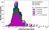 |
Fig. 2 Stacked histogram of the orbital periods of all 991 planets in the period catalogue shown for each planet multiplicity: systems with three (magenta), four (green), five (blue), and six to eight (red) detected planets. All four multiplicities have planets spanning the entire range of orbital periods from 0.32 to 170 000 days. The median of the total distribution is 12.6 days. |
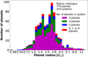 |
Fig. 3 Distribution of the radii of all 779 planets in the radius catalogue shown for each planet multiplicity as a stacked histogram: systems with three (magenta), four (green), five (blue), and six to eight (red) detected planets. The total distribution peaks in the sub-Neptune region at 2.5– 3.0R⊕ while displaying an underabundance at ≈1.8R⊕ and an abrupt decline at 3 R⊕. |
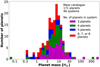 |
Fig. 4 Stacked histogram of the masses of all 171 planets in the mass catalogue shown for each planet multiplicity: systems with three (magenta), four (green), five (blue), and six or seven (red) detected planets. These are the true planetary masses which are obtained either from TTVs or via RVs in conjunction with measurements of the orbital inclinations (Sect. 2). |
3 Orbital spacings
The relative distance between two adjacent planets is expressed in this paper as the ratio of their orbital periods, Pi+ı/Pi, where Pi is the orbital period of a given planet in a system, while Pi+1 denotes the period of the next adjacent planet, indexed by increasing semi-major axis. We refer to this distance as the orbital spacing or the period ratio (PR). We have compared the observed orbital spacings to one another within the same system (on a system level) as well as across many systems (on a population level).
By examining the CKS sample, Weiss et al. (2018b) reported that the majority of adjacent planet pairs with orbital period ratios < 4 possess similar PRs (Sect. 3.2). We note that equal orbital spacings in a system correspond to equal distances in log(P) since:
 (1)
(1)
Due to detection biases and geometrical limitations, long- period planets are prone to remain undiscovered. Hence, this naturally imposes an upper limit on the orbital periods and spacings that we are able to detect. This pertains not only to outer but also inner and intermediate planets since they can be undetectable as well, for instance due to shallow transit depths or low signal-to-noise ratios. Missing an intermediate planet in a system usually creates a large spacing between the two apparently adjacent planets, thus diminishing the intra-system spacing similarity. On the other hand, undetected inner or outer planets might either increase or decrease the intra-system similarity, depending on their spacings relative to their neighbours. Consequently, if one or multiple planets in a system escape detection, the system’s true architecture and planet multiplicity are rendered incomplete.
As an example, if a solar-sized star hosts four evenly spaced planets with orbital periods of 2, 20, 200, and 2000 days (corresponding to PR = 10), the geometrical probability of detecting transits of the two outer planets is very low ranging from 0.2% to 0.7%. Therefore, in a transit survey we might only be able to detect the two inner planets in this system and thereby conclude one of the following three possibilities: (a) This system does not contain a third outer planet due to the large spacing between the two discovered planets; (b) There is an undetected intermediate planet; (c) Due to observational biases, no outer planet is detected, because its orbit has a large semi-major axis or a high inclination.
In order to diminish the effects of these observational biases, we applied different upper limits on the period ratios investigated in this work. This helps decrease the probability of missing outer transiting planets and increase the likelihood of having detected all intermediate planets in a system. In the remainder of this paper, it is explicitly stated when and which PR limits are implemented, particularly limits of 25, four, and two.
3.1 Diversity of orbital spacings
On a population level, pairs of adjacent planets in observed multi-planetary systems display a wide range of orbital spacings. This is seen in Fig. 5 which shows a stacked histogram of the distributions of all period ratios < 25 of adjacent planets in the period catalogue for each planet multiplicity. We applied an upper PR limit of 25 because the region above this threshold is sparsely populated with only 14 planet pairs possessing very high PRs up to 2662. A high period ratio may, for instance, be indicative of an undetected intermediate planet or perhaps an asteroid belt similar to the one in the Solar System (Sect. 7). The imposed upper limit of PR = 25 also serves as a first step towards decreasing the probability of undetected intermediate planets. The resulting sample consists of 282 systems with a total of 977 planets and 695 planet pairs. This is the hitherto largest sample of pairs of confirmed adjacent planets for which the PRs and the PR similarities (Sect. 3.2) have been examined.
The highest detected orbital period ratio in this selected sample is 24, which is the maximum ratio in both the radius and the mass catalogues as well (the planet pair TOI-561 b–c). As seen in Fig. 5, few detected planet pairs have very large orbital spacings. For example, only 84 planet pairs (15% of all the pairs in this sample) have PRs ≥ 4, and there is an apparent paucity at PRs ≥ 7. The smallest and highest orbital period ratio in the entire period catalogue without a PR limit is 1.17 and 2662, respectively. The absence of planet pairs with PRs < 1.17 is presumably due to chaotic orbital motion and Lagrange instability caused by overlap of first-order mean motion resonances MMRs (Deck et al. 2013). For low-mass planets with planet-to-star mass ratios of Mp/M★ ≲ 10−5, this occurs at PRs < 1.2, even if their orbits lie in a region of Hill stability (Deck et al. 2013, Fig. 12).
Furthermore, there is a weak negative correlation between the planet multiplicities and the orbital period ratios, meaning that planets tend to be more tightly packed in higher- multiplicity systems. This trend is noticeable in Fig. 5, especially for the systems with at least five planets. The 0.25-, 0.50-, and 0.75-quantiles of the PR distribution of this sample are: 1.63, 2.06, and 2.76, respectively. The median PR for the three-, four-, five-, and six to eight-planet systems is 2.16, 1.93, 1.93, and 1.63, respectively. This corroborates previous findings that planet pairs in high-multiplicity systems possess smaller orbital period ratios (Steffen & Hwang 2015). Nevertheless, it is important to note that this negative correlation is strengthened by observational biases and limitations, as discussed in Sect. 7.1.
The three strongest first-order mean-motion resonances of 4:3, 3:2, and 2:1 are marked in Fig. 5, showing that there are overabundances of planet pairs with ratios slightly greater than these MMRs as well as deficits at PRs slightly less than these MMRs. The most prominent peak in the overall distribution is near the 3:2 MMR, while the greatest trough is slightly interior to the 2:1 MMR. These near mean-motion-resonance features have been reported in previous studies of Kepler systems and found to be statistically significant (e.g. Steffen & Hwang 2015; Lissauer et al. 2011; Fabrycky et al. 2014).
To further decrease the probability of undetected planets in systems and to facilitate comparisons with Weiss et al. (2018b) and Weiss et al. (2023), we selected from the period catalogue only the pairs of adjacent planets with PRs < 4. This resulted in 611 planet pairs and is, thus, still the largest sample of PRs of confirmed planets reported in the literature. The PR distribution for each planet multiplicity is displayed in Fig. 6 on a linear scale. This enabled us to mark the corresponding values for all seven adjacent planet pairs in the Solar System, except for Mars-Jupiter which have a high PR of 6.3. The remaining six pairs have PRs ranging from 1.6 for Venus-Earth to 2.8 for Saturn- Uranus and are, therefore, typical among the exoplanet pairs, as also noted for instance by Malhotra (2015). By applying an upper PR limit of 4, the planet multiplicity and orbital period ratios are slightly more strongly correlated, leading to Pearson-R = −0.19 as opposed to Pearson-R = −0.14 for the previous sample with PRs < 25.
Furthermore, we computed several sets of both Anderson- Darling and Kolmogorov-Smirnov tests in order to assess whether the four multiplicity distributions of PRs are significantly different or can be drawn from the same population. The following conclusions are the same both when applying no upper PR limit and with a limit of either 4 or 25. The sets of both types of tests indicate that the three-planet systems are drawn from a different distribution of PRs (i.e. skewed towards larger values) than the systems with a minimum of four planets. However, there is not yet sufficient data to study whether this pattern extends to higher multiplicities.
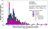 |
Fig. 5 Distribution of the orbital PRs of pairs of adjacent planets in the period catalogue up to a PR limit of 25 shown for each planet multiplicity as a stacked histogram: systems with three (magenta), four (green), five (blue), and six to eight (red) detected planets. This sample contains 695 planet pairs, thereby excluding 14 pairs with 25 < PRs < 2662. Adjacent planets in higher-multiplicity systems tend to have smaller PRs. There are overabundances of PRs slightly greater than the 4:3, 3:2, and 2:1 MMRs (Sect. 3.1). |
3.2 Similarity of adjacent orbital spacings
In contrast to the diversity of period ratios exhibited by the pairs of adjacent planets on a population level in Fig. 5, the orbital spacings within an individual system tend to be equal (e.g. Weiss et al. 2018b; Jiang et al. 2020). This means that planets orbiting the same star tend to be equally spaced in logperiod (Eq. (1)). This intra-system uniformity is a key feature of the peas-in-a-pod architecture in addition to the similarities of the planetary sizes and masses as well as the low orbital eccentricities and mutual inclinations in a system. Previous studies analysing Kepler data have determined that the spacing similarity trend is not caused by detection biases or limitations and is, therefore, not an artefact of Kepler’s discovery efficiency (Weiss & Petigura 2020; Mishra et al. 2021; Weiss et al. 2018b, 2023; He et al. 2019; Jiang et al. 2020; Lammers et al. 2023). Furthermore, population synthesis models of planetary systems have revealed that the intra-system spacing similarity is a typical outcome of system formation and evolution (Mishra et al. 2021, 2023b; Weiss et al. 2023). It has also been shown that this spacing trend is diminished in observations due to the biases and limitations of the transit method as well as the completeness of the Kepler survey (Mishra et al. 2021).
In order to investigate the spacing similarity in a system with N planets, the period ratios of all pairs of adjacent planets need to be compared: Pi +1/Pi for i = 1,2,…, N. The standard approach employed in previous work is to plot Pi+2/Pi+1 against Pi+1/Pi for all adjacent planet pairs and test for a correlation. The points representing a system in which all adjacent planets have equal PRs lie perfectly on top of each other at a certain value on the one-to-one line in such a plot.
Despite their simplicity, correlation tests are only suitable for large datasets and cannot be applied on a single planetary system (i.e. on a system level). This is due to the very low number of data points, since N planets result in N − 1 planet pairs and only N − 2 points to plot. Therefore, in order to exploit the advantages of correlation tests, all the adjacent planet pairs in all the systems should be plotted on the same graph (i.e. on a population level). The disadvantage, however, is that information about an individual system is lost since we do not know which data points correspond to the same system. In order to measure the similarity on a system level, we therefore employed another method as explained in Sect. 3.3.
Figure 7 displays the orbital period ratio of a pair of adjacent planets Pi+2/Pi+1 vs. the PR of the previous such pair Pi+1/Pi in the period catalogue. We selected the systems with at least two adjacent planet pairs with PRs < 25. This sample is slightly smaller than the one displayed in Fig. 5 but is still the largest for which the spacing similarity has been examined thus far. It contains 272 systems with a total of 957 planets, 685 planet pairs, and 413 data points. The previously largest sample was analysed by Weiss et al. (2018b) who selected from the CKS multis the systems with a minimum of three candidates or confirmed planets in which at least two adjacent planet pairs had PRs < 4. This resulted in 104 systems with a total of 373 planets and 165 data points. Their sample is, therefore, significantly smaller than the one we investigated in this work.
Figure 7 also displays the corresponding values for the inner Solar System (the four terrestrial planets) and the outer Solar System (the four giant planets). These planet pairs do not have equal orbital spacings but are, nonetheless, typical among the other pairs, tending to follow the one-to-one line.
There is a significant positive correlation between the orbital period ratio of a pair of adjacent planets and the PR of the next such pair in the same system. However, the upper limit on the period ratios affects the strength of this correlation. With no upper PR limit for the CKS multis, Weiss & Petigura (2020) found a weak positive correlation that was barely significant (p-value = 0.003). Notwithstanding this result, Jiang et al. (2020) identified no correlation at all for the Kepler systems with a minimum of three candidates (including confirmed planets) after applying a limit on the planetary radii of 6 R⊕ and no limit on the period ratios. Recently, also Mamonova et al. (2024) found no correlation between the orbital PRs of adjacent planets in their sample of observed multi-planetary systems. Contrary to the aforementioned studies, our analysis suggests that a correlation does in fact exist even when large orbital period ratios up to 2662 are included.
Additionally, we investigated how the upper PR limit alters the correlation statistics for our sample. The linear correlation coefficient for the entire period catalogue with 1.17 < PRs < 2662 is Pearson-R = 0.20, after which it increases to its maximum value of Pearson-R = 0.31 for 1.17 < PRs < 25. By further decreasing the upper PR limit, the correlation coefficient fluctuates between 0.26 and 0.31 until PRs < 1.7 at which the p-value becomes insignificant.
It is visible in Fig. 7 that the majority of points get farther away from the 1:1 line as the period ratios increase, implying that the correlation is diminished at high orbital spacings. Noticeably, there is an absence of points in the upper right corner of this figure. This is primarily caused by observational biases because two adjacent planet pairs are most likely undetectable if they both have very high PRs. In this region, the correlation statistics are, therefore, misrepresented, which is the reason why proper PR limits are needed. As seen in Fig. 7, especially data points at PRs > 4 are largely dispersed relative to the 1:1 line, and a very large orbital spacing in one planet pair is mainly associated with a much smaller spacing in the adjacent pair, since otherwise both pairs might not have been detected.
Therefore, in order to mitigate these effects of observational biases and, thereby, decrease the probability of intermediate and outer undetected planets, we imposed an upper PR limit of 4, as implemented in Weiss et al. (2018b). The resulting sample acquired from the period catalogue contains 217 systems with a total of 765 planets and 548 planet pairs, fulfilling that PRs < 4 for every two adjacent planet pairs. Figure 8 shows the similarity of the adjacent orbital spacings in this sample (331 data points) along with the corresponding plot (165 data points) presented in Weiss et al. (2018b). Although the correlation in our sample is weaker than in Weiss et al. (2018b), it is more significant and indicates that the peas-in-a-pod spacing pattern at PRs < 4 emerges even in a sample twice as large.
Another distinctive feature in both Figs. 7 and 8 is the near symmetry along the one-to-one line. The data points (x, y) are approximate reflections of each other across this line. Moreover, this property is independent of the number of planets in the systems. There is no correlation between the planet multiplicity and whether x < y, or y < x; that is, whether the inner or outer planet pair has a higher period ratio. This near symmetry about the 1:1 line emerges both owing to the peas-in-a-pod planets that lie along this line as well as due to observational biases since a large PR in a planet pair necessitates a much smaller PR in the adjacent pair in order for both pairs to be detected.
Since planets in higher-multiplicity systems tend to be more tightly packed (Sect. 3.1), we focused next exclusively on the systems in the period catalogue with a minimum of four planets. We conducted the same analysis and examined the spacing similarities as in Fig. 7. The results indicate that irrespective of the upper PR limit, the correlation between the orbital period ratios of adjacent planet pairs is weaker in this sample that excludes the three-planet systems.
In order to explore how the planets detected only with the RV method influence the spacing similarity trend, we examined the planets in the radius catalogue since they all have been detected by transit photometry. TOI-561 b–c is the planet pair with the highest PR of 24, which is the same as in Fig. 7 for the period catalogue limited to PRs < 25. The correlation between adjacent PRs has now the coefficient Pearson-R = 0.21 and is, therefore, weaker compared to the previous Pearson-R = 0.31. For the planet pairs with PRs < 4, the Pearson-R is 0.27 and 0.30 for the radius and period catalogue, respectively. These two results have two main implications: First, the planets detected with the RV technique increase the strength of the spacing similarity trend (for PRs < 25). Second, they predominantly affect the correlation at PRs > 4 since the majority of them have larger orbital spacings than the transiting planets.
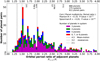 |
Fig. 6 Similar to Fig. 5 but for all 611 pairs of adjacent planets in the period catalogue with PRs < 4 shown on a linear scale. The uppercase letters at the top mark the PR values of all adjacent planet pairs in the Solar System, apart from Mars-Jupiter with PR = 6.3. |
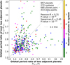 |
Fig. 7 Period ratio of a pair of adjacent planets versus the PR of the previous such pair for all 685 pairs in the period catalogue where every two adjacent pairs have PRs < 25. Hence, each data point represents two adjacent planet pairs, resulting in 413 points colour-coded based on the planet multiplicity in each system. There is a positive correlation, although the points are greatly dispersed around the 1:1 line. Points representing planet pairs in a system where there is a perfect spacing similarity lie precisely on top of each other on this line. The two black stars and diamonds mark the planet pairs in the inner and outer Solar System, respectively (Sect. 3.2). |
3.3 Intra-system similarity of orbital spacings
While statistical correlation tests, such as the Pearson and Spearman tests, are applicable on large datasets in population-level research, they are not suitable for measuring distinctive trends within an individual system. Therefore, other appropriate tests or measures must be devised in order to examine the intra-system properties and correlations. There are only a few system-level studies reported in the literature (Kipping 2018; Gilbert & Fabrycky 2020; Goyal & Wang 2022; Mishra et al. 2023a; Weiss et al. 2023; Mamonova et al. 2024).
In this work, we employed a straightforward metric that quantifies the similarity of a specified parameter, as for instance the orbital spacings or the planet masses within an individual system. This facilitates both intra- and inter-system analyses of multi-planetary systems. Similar to Weiss et al. (2023)’s approach, we implemented the fractional dispersion, which is the standard deviation σq of a quantity q defined as follows:
 (2)
(2)
where N designates the number of planets in the system and is ≥3. The log-base is set to 10, and  denotes the mean of the quantity q in the system.
We applied Eq. (2) on the orbital period ratios (σPR) as well as the planetary radii (σR; Sect. 4), masses (σM; Sect. 5), and Hill radii separations (σΔ; Sect. 6). σq defined in this work is dimensionless and can range from 0 up to very large numbers. Henceforth, σPR is referred to as the spacing dispersion or, equivalently, as the dispersion of period ratios or of spacings. If all the planets in the same system resemble peas in a pod, they display a small dispersion and, thereby, a strong intra-system similarity.
We also quantified the intra-system similarity by computing the coefficient of variation,  , which is defined as the standard deviation of a quantity q divided by the mean q of a dataset (Brown 1998). The results from the two metrics utilised in our analyses are consistent with one another, and henceforth we only report on the spacing dispersion σPR.
It is important to note that a compact system has planets with short orbital periods but does not implicitly exhibit a low spacing dispersion. This also means that if adjacent planets in a non-compact system have high but nearly equal period ratios, the resulting spacing dispersion is low. However, due to observational limitations, the outer planets in non-compact systems are prone to remain undetected.
We computed the spacing dispersions in all 282 systems in the period catalogue in order to identify common architecture trends. The five systems with the lowest dispersions, ranging from 0.00047 to 0.00084, are in increasing order: Kepler-398, Kepler-229, Kepler-271, Kepler-207, and Kepler-289. In the opposite extremity, the five largest dispersions range from 0.85 to 1.99 and belong to the following systems in increasing order: GJ 433, Kepler-88, HD 181433, HD 27894, and HD 153557. It is noteworthy that each of these five systems contain at least one long-period planet detected by RVs (Sect. 7.3). As a comparison, the dispersion of orbital spacings in the inner, outer, and entire Solar System are 0.082, 0.068, and 0.18, respectively. Hence, our host system has an intermediate value and is typical among the discovered multi-planetary systems in terms of the intra-system spacing similarities. However, when comparing only the inner regions of systems with inner transiting planets and minimum one outer giant, the inner Solar System possesses the smallest spacing dispersion (Sect. 4).
Disregarding observational biases, from the above examinations of spacing dispersions we can highlight two main results that apply on the observed systems in our catalogue. First, the majority of systems with very large dispersions contain one pair of adjacent planets that has a much higher period ratio than all the other pairs in its respective system. Second, there is neither a Pearson nor a Spearman correlation between the spacing dispersions and the planet multiplicity in the systems. This is also in agreement with our results from the Anderson-Darling and Kolmogorov-Smirnov tests, indicating that the dispersion distributions for all four planet multiplicities can be drawn from the same population.
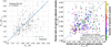 |
Fig. 8 As in Fig. 7 but now only for PRs < 4. Left figure: graph from Weiss et al. (2018b) displaying 165 data points from a total of 104 systems and 373 planets. This has been the largest observed sample for which a strong similarity of adjacent spacings has been found. Right figure: sample from the period catalogue in this work comprising 331 data points from a total of 217 systems, 548 planet pairs, and 765 planets. Although this sample is smaller than that in Fig. 7, it is twice as large as that of Weiss et al. (2018b) and shows a weaker, but more significant, correlation. |
4 Relations between planet size and spacing
In this section, we first examine whether the intra-system similarity of orbital spacings is connected to that of the planetary radii. Then we explore whether the previously reported correlation between period ratios and planetary radii emerges in our sample.
The dispersion of planetary sizes in a system indicates how similar the planets are in terms of their radii R. We used the metric given in Eq. (2) and computed σR , where the radii are in units of Earth radii R⊕. We remind that this metric measures the radii in log-space, and therefore it actually implements the ratios and not the differences between the planets’ radii and the mean value in a system.
We investigated whether there exists a correlation between the intra-system dispersion of orbital spacings and that of planetary sizes. When including all 225 systems from the radius catalogue, the Pearson and Spearman tests indicate a weak positive correlation between the two dispersions σR and σPR . Next, we performed the similar tests on different sub-samples and examined whether the relation between the two dispersions changes.
Our analyses indicate that the correlation diminishes significantly with a decreasing upper PR limit; that is, when we selected the systems in which all pairs of adjacent planets have PRs smaller than the specified limit. Surprisingly, the correlation between the two dispersions vanishes completely already at an upper PR limit of 6. Figure 9 displays the size dispersions vs the spacing dispersions in the 206 systems (out of 225) from the radius catalogue in which all the pairs of adjacent planets have PRs < 6. This may suggest that for nearly all the transiting- planet systems, the intra-system dispersion of the planetary sizes is uncorrelated with that of the orbital spacings.
Figure 9 also shows the corresponding values for the inner and outer Solar System. They resemble the other systems in the sample and have typical spacing dispersions of 0.08 and 0.07, respectively, but larger size dispersions of 0.18 and 0.22. On the contrary, the entire Solar System cannot be encompassed in this figure due to its large size dispersion of 0.60 even though its spacing dispersion is only 0.18.
In order to perform a more adequate analysis for the inner Solar System, we compared it only to other inner planetary systems. We selected the systems in the period catalogue that contain minimum three inner transiting planets with R < 9 R⊕ (i.e. smaller than giant planets) and at least one outer massive planet with M sin i ≥ 50 M⊕ (following the threshold in He & Weiss 2023). There are five such systems of which Kepler-139 and Kepler-65 each have three inner planets and one outer giant. The other three systems are: Kepler-48 with three inner planets and two outer giants, Kepler-90 with seven inner and one outer planet, and HD 191939 with three inner planets and two outer giants. The size and spacing dispersions of the inner planets in each of these systems are marked in Fig. 9 with black squares, except for Kepler-139 since its inner planets exhibit a very large spacing dispersion of 0.35, thus exceeding the domain of the graph. All five inner systems have larger spacing dispersions than the inner Solar System, but except for Kepler-90, they all have smaller size dispersions. This is further discussed in Sect. 7.3.
As seen in Fig. 9, many of the systems in the radius catalogue exhibit an intra-system similarity in orbital spacings and/or planet sizes. K2-183 has the greatest spacing dispersion of σPR = 0.58, which could easily be decreased if an additional planet would be discovered between planet b and c, since these two planets have a high period ratio of 23. Kepler-1311 has the largest size dispersion of σR = 0.47 as well as a high spacing dispersion of σPR = 0.32. The high period ratio of 18 between planet b and d might indicate that there is an undetected planet between them.
In order to decrease the probability of undetected intermediate planets, we next examined the systems in which all pairs of adjacent planets have PRs < 2. By choosing this low PR limit we assume that there are no undetected planets between the inner- and outermost planet in each of these systems. This selection resulted in 51 systems with a total of 179 planets, which are bordered by the red lines in Fig. 9. Evidently, the two dispersions in this sub-sample are not correlated, and all these systems possess small spacing dispersions but span a wide range of size dispersions. This suggests that planets in the same system can have similar orbital spacings even if they are not similarly sized.
As a supplement to the dispersion of sizes and spacings within each system, the relationship between planetary radii and orbital spacings may also be explored on a population level for all pairs of adjacent planets in the sample. Weiss et al. (2018b) identified a weak positive correlation between the average radii and the orbital period ratios of adjacent planets, which we henceforth refer to as the size-spacing correlation. Their sample comprised all 504 adjacent planet pairs in the CKS multis, of which approximately half are in two-planet systems. This relationship is likely to have an astrophysical origin since it also exists in an underlying unbiased synthetic population (Mishra et al. 2021; Weiss et al. 2023). Moreover, its strength is shown to diminish due to the biases and limitations of the transit method as well as the completeness of the Kepler survey (Mishra et al. 2021).
We investigated whether this size-spacing correlation emerges in our radius catalogue as well, since it comprises more planet pairs (554) than the CKS multis and does not contain neither unconfirmed planets nor systems with only two planets. The resulting relationship is seen in Fig. 10 where each point represents a pair of adjacent planets and is colour-coded by the number of planets in the system. There is a very weak positive correlation with Pearson-R = 0.17 (p-value <10−4). This coefficient remained unchanged even when we excluded the planet pairs with PRs > 4 in order to decrease the probability of undetected intermediate planets.
The most prominent features in Fig. 10 are that small planet pairs with average radii R < 1.1 R⊕ have predominantly small period ratios of PRs < 1.7. Conversely, large planets with R > 4R⊕ tend to possess larger PRs, while intermediate-sized planet pairs span a wide range of orbital spacings and reveal no apparent pattern.
As noted by Weiss et al. (2018b), there is a noticeable absence of planet pairs with average radii < 1R⊕ at large orbital period ratios. When we selected from the radius catalogue the 21 planet pairs in this size range, we found a typical value of PR ≤ 2, which is in agreement with Weiss et al. (2018b). This implies that the vast majority of small-sized planets are in tightly packed configurations. The latter authors also determined from bootstrap models that planets smaller than 1R⊕ are in fact detectable at period ratios up to four. Their conclusion was that the lack of such planets with period ratios of 2 < PRs < 4 likely has an astrophysical origin. They identified a stronger correlation when examining only the planet pairs with average radii < 1R⊕. In contrast to this result, we found no correlation between the PRs and average sizes of the 21 planet pairs with average R < 1R⊕ in our radius catalogue.
We also tested how excluding these 21 planet pairs affects the planet size-spacing trend, first with no upper PR limit and then with a limit of 4. The conclusions from both these approaches are consistent with one another, revealing that there is no correlation between the average radii and the period ratios in this sub-sample. This implies that the correlation between the sizes and PRs of adjacent planets shown in Fig. 10 disappears when planet pairs with average R < 1R⊕ are excluded. Only when we additionally excluded planet pairs larger than 4R⊕ did a significant, but very weak, correlation emerge, which then increased with decreasing upper limit on the radius. These results may have two implications: Firstly, for planets with radii of 1R⊕ ≤ R ≤ 4R⊕, the orbital period ratios tend to be larger as the planets’ radii increase. Secondly, planets with R > 4R⊕ show no preference for their orbital spacings based on the planet size.
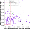 |
Fig. 9 Size dispersion σR versus spacing dispersion σPR (Eq. (2)) of all pairs of adjacent planets in a system. This shows the 206 systems from the radius catalogue in which all adjacent planet pairs have PRs < 6. There is no correlation between the two dispersions. Among the points enclosed by the red lines, there are 51 systems in which all PRs < 2. The black squares represent the inner regions of five systems that contain a minimum of three inner small planets and at least one outer giant. Both the inner Solar System (square) with the terrestrial planets and the outer Solar System (triangle) with the four giants possess typical dispersions (Sect. 4). |
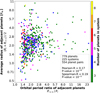 |
Fig. 10 Average radii versus orbital period ratios of all 554 pairs of adjacent planets in the radius catalogue. Each point is colour-coded based on the number of planets in the system. There is a weak positive correlation that breaks down when planet pairs with average radii <1 R⊕ are excluded. Very small and very large planet pairs have predominantly small and moderate PRs, respectively, while the intermediate planets span a much wider range of orbital spacings (Sect. 4). |
5 Relations between planet mass and spacing
The observed relationships between planetary sizes and orbital spacings likely originate from underlying relationships between the masses and spacings of planets. To explore this, we used the sample in the mass catalogue and conducted the same analyses as in the previous section focusing on the planetary masses instead. This has not been pursued in previous studies on observed data although Mishra et al. (2021) examined the masses vs. the period ratios of a synthetic planet population.
We focused exclusively on the mass catalogue since we wanted to utilise the planetary masses M and not M sin (i) measurements or values obtained through mass-radius relationships. First, we investigated the intra-system similarities using Eq. (2), and the mass dispersions σM vs. the spacing dispersions σPR of all 46 systems are plotted in Fig. 11.
The inner and outer Solar System have σM = 0.61 and σM = 0.64, respectively, and are shown in the figure as well. Only four systems have mass dispersions larger than these two values. Meanwhile, the entire Solar System has a very large value of σM = 1.73 and cannot be encompassed in Fig. 11.
Similar to our procedure in Sect. 4, we selected the five systems in the period catalogue that contain at least three inner transiting planets and a minimum of one outer giant. Only three out of these systems have true mass values for all their inner planets: HD 191939, Kepler-48, and Kepler-65. The mass and spacing dispersions of the inner regions of these systems are marked in Fig. 11, showing that they have larger spacing dispersions but smaller mass dispersions compared to the inner Solar System.
Although the number of systems is not statistically large, our analysis indicates that the two dispersions are not correlated. This result agrees with our conclusions in Sect. 4 and solidifies our finding that planets in the same system can be similarly spaced even if they do not have similar sizes or masses. To test this idea further, we proceeded as in Sect. 4 and examined the systems in which all pairs of adjacent planets possess PRs < 2. Thus, we assume that these systems have tightly packed planets without any undetected intermediate planets. There are only 12 such systems (marked in Fig. 11) compared to the 51 systems in the radius catalogue. In contrast to their small spacing dispersions, they clearly display much larger mass dispersions, particularly the four systems with σM > 0.26. This is in agreement with the trend in planet size in Fig. 9 but is more pronounced for the planet mass.
Kepler-60 is the system with the smallest dispersions in the lower left corner of Fig. 11, exhibiting a peas-in-a-pod architecture for both mass and spacing. The systems with the highest and next-highest spacing dispersions are TOI-561 and Kepler-62, respectively, although both the radius and period catalogues contain systems with larger dispersions. Systems with large σPR might harbour undetected intermediate planets, especially if they display small σM values.
Complementary to focusing on each system individually, we investigated all 125 pairs of adjacent planets in the mass catalogue. The average mass as a function of the orbital period ratio of each pair is displayed in Fig. 12. Massive planets, in particular with average M > 10 M⊕, tend to have larger PRs than low-mass planets. The orbital spacings are more strongly correlated with the planetary masses than with the radii (Fig. 10), and both the Pearson and Spearman coefficients are higher. Comple-mentarily, in a synthetic population of multi-planetary systems, Mishra et al. (2021) identified a stronger linear correlation of the PRs with the masses than with the radii of planets. For the first time we investigated and corroborated this result in a sample of detected planets with true mass values. We note, however, that the data sample in Fig. 10 is almost 4.5 times larger compared to the one presented in Fig. 12, although the correlations are significant in both samples.
In the mass catalogue, the planet pair TOI-561 b–c has the highest period ratio of ≈24, since planet b is an ultra-short-period planet, while planet c has an orbital period of ≈11 days. As seen in Fig. 12, the majority of planet pairs in systems with ≥5 planets have average masses of M < 10 M⊕ and small orbital spacings irrespective of their masses. Both the PRs and masses are small for all the planet pairs in the TRAPPIST-1 system. Two of the four planet pairs with masses M > 100 M⊕ orbit Kepler-30, while the other two reside in the WASP-47 system.
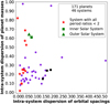 |
Fig. 11 Mass dispersions σM versus spacing dispersions σPR (Eq. (2)) for all 46 systems in the mass catalogue. There is no correlation between the two dispersions. The 12 systems in which all PRs < 2 (star symbols) have small spacing dispersions but span a wide range of mass dispersions. Both the inner and outer Solar System have large mass dispersions. The black squares correspond to the inner regions of three systems that contain at least three inner small planets and a minimum of one outer giant (Sect. 5). |
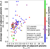 |
Fig. 12 Average mass versus orbital period ratio of every two adjacent planets in the mass catalogue. There is a weak Pearson and a moderate Spearman correlation, which are much higher than in Fig. 10. Each point is colour-coded based on the planet multiplicity in the system. The majority of planet pairs in systems with ≥5 planets have small PRs and average masses of M < 10 M⊕. |
6 Mutual Hill radii separations
Planets interact gravitationally with each other, implying that larger and more massive planets necessitate wider mutual separations compared to their smaller counterparts. Each planet has its own radius of gravitational influence, denoted as its Hill radius, where its influence dominates over that of the host star. For two adjacent planets with masses Mi and Mi+1 this can be represented by their mutual Hill radius defined as

where ai and ai+1 are the semi-major axes of the planets’ orbits around their host star with mass M★. The orbital separation Δ between two adjacent planets is given in units of their mutual Hill radius:
 (3)
(3)
Is the fundamental orbital spacing between two adjacent planets best represented by their period ratio Pi+1/Pi or their separation Δ? We concluded in Sect. 3.2 that adjacent planets in the same system often have similar orbital period ratios, as revealed in Fig. 7. We ask now whether this trend might in fact emerge from an underlying similarity of these planets’ separations Δ (cf. Weiss et al. 2018b). As defined in Eq. (3), the mutual Hill radii separations depend partly on the semi-major axes and are, therefore, related but not directly proportional to the period ratios. For instance, even if two pairs of adjacent planets have equal period ratios, the pair with the less massive planets has a larger separation Δ.
In this section we investigate whether the orbital spacings between adjacent planets are more similar in terms of their period ratios or Hill radii separations. Figure 13 shows the distribution of Δ of all the 125 pairs of adjacent planets in the mass catalogue. Apart from the pair TOI-561 b–c with Δ = 75, the smallest and largest separations are Δ = 5.7 and 41, respectively. The values for all seven pairs of adjacent planets in the Solar System are marked in Fig. 13. All three planet pairs in the inner Solar System have larger separations than the four remaining pairs. Although Mars and Jupiter have the largest PR of 6.3, Mercury and Venus have the largest separation of Δ = 63.
As seen in Fig. 13, there is a negative correlation between the planet multiplicity and the separations Δ. This corroborates previous findings showing that planets in high-multiplicity systems are more dynamically packed than in lower-multiplicity systems (e.g Fabrycky et al. 2014; Pu & Wu 2015; Weiss et al. 2018b).
The total distribution has a median of Δ ≈ 15 and a mean of Δ ≈ 17, while peaking around Δ ≈ 12. These values are in agreement with the results of Pu & Wu (2015), who evaluated the separations Δ in Kepler systems with four, five, and six candidates.
We investigated whether the spacing similarity trend is more pronounced in units of orbital period ratios (Fig. 7) or mutual Hill radii by comparing the standard deviations σPR to σΔ for all 46 systems in the mass catalogue. These are shown in Fig. 14 along with the values for the inner, outer, and the entire Solar System. We find that most of the systems lie above the one-to-one line in the figure, implying that they have planets that are more dispersed in Δ than in period ratios. This suggests that the orbital spacings between adjacent planets are more similar in units of period ratios than of mutual Hill radii.
Figure 14 also displays the values for the inner transiting planets in each of the three systems: HD 191939, Kepler-48, and Kepler-65, as in Fig. 11. Although the inner Solar System possesses a smaller spacing dispersion compared to these systems, its dispersion of Δ is slightly larger than that of Kepler-48.
Finally, as in Sect. 5 we examined the 12 systems in which all the pairs of adjacent planets have PR < 2, as marked with star symbols in Fig. 14. These systems harbour planets that we consider to be so tightly packed that no intermediate planets can have stable orbits. Although these systems have low period ratio dispersions σPR, they span a wide range of separation dispersions σΔ. This supports our conclusion that the intra-system spacing similarity is more pronounced in units of orbital period ratios than of mutual Hill radii separations.
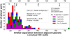 |
Fig. 13 Stacked histogram displaying the distributions of orbital separations Δ (in units of mutual Hill radii) of all 125 pairs of adjacent planets in the mass catalogue shown for each planet multiplicity: systems with three (magenta), four (green), five (blue), and six or seven (red) detected planets. The separations tend to be smaller in high-multiplicity systems. The planets TOI-561 b and c have the largest mutual separation of Δ = 75. The uppercase letters at the top mark the values of all the adjacent planet pairs in the Solar System (Sect. 6). |
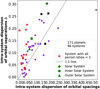 |
Fig. 14 Dispersion of orbital separations Δ versus the dispersion of PRs between adjacent planets in each of the 46 systems in the mass catalogue. The majority of systems display greater dispersions of separations Δ than of PRs, and the upper right outlier is the TOI-561 system. The 12 systems (star symbols) in which all PRs < 2 have small PR dispersions but span a wide range of Δ dispersions. Both the inner and outer Solar System have typical dispersions, while the entire Solar System has greater values. The black squares represent the inner regions of three systems that contain a minimum of three inner small planets and at least one outer giant. |
7 Discussion
In this section we consider the impact of observational biases in our data and discuss some of the results and limitations of our analyses.
7.1 Detection biases and limitations
Throughout our work we have considered how the limitations and biases of the transit and RV surveys might affect our analyses. Since 794 out of all the 991 planets in the period catalogue have been discovered using the transit method, the geometrical limitations and detection biases of this technique could play a key role. If unaccounted for, observational biases might distort the following five underlying properties: the similarity of adjacent spacings, the intra-system spacing dispersion, and the relationships between the spacings and the planets’ sizes, masses, and multiplicities.
Observational biases might cause planets in a system to remain undetected. This could for instance occur in transit surveys if these planets have high mutual inclinations and are not seen transiting their star. Mishra et al. (2021) showed that both the spacing similarity and the size-spacing trends are diminished by the biases and limitations of the transit method as well as the completeness of the Kepler survey.
For example, we can consider a hypothetical system of five planets with orbital periods of 1, 4, 16, 64, and 256 days. The inner three planets are equally sized, while the outer two planets are much larger. The period ratio between all pairs of adjacent planets is four and is, thus, uncorrelated with the planet size. We further consider that Kepler has observed this system, but that the planet at 64 days is not transiting. Hence, what we actually detect is a four-planet system in which the two inner pairs of adjacent planets have similar sizes and period ratios of four, whereas the outer planet pair has a larger average size and a period ratio of 16. This observational bias has five erroneous effects:
- (a)
It renders our observation sample incomplete.
- (b)
It strengthens the negative correlation between planet multiplicity and period ratios (Sect. 3.1).
- (c)
It diminishes the similarities of adjacent spacings (Sect. 3.2).
- (d)
It increases the intra-system spacing dispersion (Sect. 3.3).
- (e)
It increases the positive correlation between planetary sizes and period ratios (the size-spacing trend; Sect. 4).
In other cases instead of being strengthened, the size-spacing correlation might on the contrary be weakened by detection biases. This could occur if small-sized tightly packed planets remain undetected due to their very shallow transit depths while larger and more widely spaced planets are observed.
As seen in Fig. 7, the similarity of adjacent spacings strongly decreases at high orbital period ratios. This feature is likely strengthened by missing intermediate planets. Furthermore, the majority of planets with high PRs have long orbital periods, and the probability of detecting these planets transiting is low. We are, therefore, biased against detecting planet pairs with similar spacings if their PRs are high. This limitation also makes our dataset incomplete and strengthens the negative correlation between planet multiplicity and orbital spacings.
Taking the above considerations into account, we analysed several data samples from our catalogues specifying different lower and upper PR limits. In order to mitigate the detection biases, in particular the effects of undetected intermediate or outer planets, we decreased the upper PR limit incrementally from 2662 down to 2 in our analyses in Sects. 3–6. For instance, in Sect. 3.2 we examined how the large PRs in the period catalogue influence the similarity trend of adjacent spacings. In contrast to Jiang et al. (2020), we concluded that this trend extends to high PRs > 4 and even up to PR = 2662 as long as all PRs down to 1.7 or less are included.
As another example, we investigated in Sect. 4 how the high PRs impact the correlation between the dispersions of planetary sizes and spacings. For the 206 systems from the radius catalogue in which all the pairs of adjacent planets have PRs < 6, there is no correlation between the intra-system dispersions of the planetary radii and those of the period ratios. However, including the remaining 19 systems in which one pair of adjacent planets possesses PR > 6, erroneously gives rise to a positive correlation. These high PRs might be caused by detection biases, and therefore we do not consider this correlation to have an astrophysical origin.
7.2 System-level analyses
Previous studies have often used correlation tests in order to investigate common architecture trends across many systems, as for instance in Figs. 8 and 10 (e.g. Weiss et al. 2018b, 2023; Jiang et al. 2020; Mishra et al. 2021). In such analyses either the planets or the planet pairs from all the systems in a sample are tested collectively. This is very efficient on large datasets and can reveal common patterns on a population level. However, this approach is no longer suitable if we want to compare the architecture of one system to that of another, since it does not enable us to keep track of each individual system. This is noticeable for instance in Fig. 7 showing the correlation between every two adjacent spac-ings for a total of 685 planet pairs. Owing to the large number of data points, the correlation is statistically significant and is ideal for examining the similarities of all the adjacent spacings in the sample. Nevertheless, for the systems with more than three planets, it is not evident in Fig. 7 which of the points represent the same system. Therefore, we cannot fully characterise the spacing similarity within an individual system using this correlation test alone.
Hence, a few other approaches have been adopted in system-level studies (e.g. Gilbert & Fabrycky 2020; Goyal & Wang 2022; Weiss et al. 2023; Mishra et al. 2023a). These have applied different metrics to measure specific properties within a planetary system or to characterise its architecture. In this work we used Eq. (2) to quantify the intra-system dispersion of each of the following quantities: the planet radii, the planet masses, the period ratios of adjacent planets, and their Hill radii separations. Naturally, each of these various approaches provides its own advantages and limitations that should be considered.
One common weakness for the metrics found in the literature is that they do not take into account the type of system that is being examined, for instance with respect to the planet masses or sizes in the system. In particular, low- and high-mass systems probably correspond to two different classes of systems, as indicated by previous research (e.g. Morrison & Kratter 2016; Emsenhuber et al. 2023; Jiang et al. 2023; Wang 2017). Therefore, it might not always be correct to apply the same metric on two different types of systems; for example on a system with low-mass and tightly packed planets as well as on a system that has both inner low-mass planets and outer giants. All the metrics utilised in past studies would indicate a higher degree of intra-system similarity for the low-mass system, especially with respect to planet size and mass. For instance, in a forming low-mass system with pairs of adjacent planets with masses <40 M⊕, theoretical research has shown that energy optimisation leads to nearly equal-mass planets in circular and coplanar orbits, when subjected to conservation of angular momentum, constant total mass, and fixed orbital spacings (Adams et al. 2020; Adams 2019). Hence, in a low-mass system a peas-in-a-pod architecture is energetically favoured over an architecture with high mass dispersion. On the other hand, in a high-mass system with a planet pair of mass ≳40 M⊕, energy optimisation leads to a configuration in which one planet undergoes runaway growth and acquires most of the mass (Adams et al. 2020). This greatly reduces the intra-system similarity of planet sizes and masses.
We must, therefore, be cautious when exploring common architecture trends using the same metric on all systems. For this reason, we investigated whether the conclusions presented in Sects. 4 and 5 hold true when dividing the systems into different classes and examining each class separately. We selected from the radius catalogue the following four categories of systems:
Systems in which all planets have R ≤ 2R⊕.
Systems that have minimum one planet with R > 2 R⊕.
Systems in which all planets have R ≤ 3.5R⊕.
Systems with a minimum of one planet with R > 3.5 R⊕.
This enabled us to examine the four system classes separately and apply the same metric as in Sect. 4 in order to measure the intra-system similarities. The results for the four system types are consistent both with each other and with our previous conclusions regarding the correlations between the planetary radii and spacings as well as the relations between their intra-system dispersions. This justifies our initial analyses of the systems in the radius catalogue without dividing them into different classes based on the planets’ radii.
We also conducted similar investigations on the systems in the mass catalogue. We divided them into two categories: one comprising the low-mass systems in which all planets have M < 10 M⊕ and another one containing all the remaining systems in the catalogue. The results from the analyses within each system class are in agreement both with one another and with our assertions in Sect. 5. This supports our initial conclusions drawn without dividing the systems into different classes.
We underline that a system’s architecture is dependent not only on its planets’ masses and sizes but also on its age and dynamical evolution. In a population synthesis experiment, Mishra et al. (2021) and Weiss et al. (2023) found that the vast majority of planet pairs possess small period ratios at early times ≲3 Myrs of planet formation. Their PRs increase during the subsequent 100 Myrs due to dynamical N-body interactions. The size-spacing correlation and the spacing similarity trend are absent at early times and emerge later over timescales of millions of years due to the dynamical sculpting in the systems (Mishra et al. 2021; Weiss et al. 2023; Lammers et al. 2023). These dynamical encounters lead to planet–planet scattering, merger collisions, or even ejections of planets, thereby increasing the orbital spacings between adjacent planets (Mishra et al. 2021). Large, massive planets have likely undergone more collisions, especially mergers, in the past than the small planets in the same system, thereby clearing more space around them. This may explain why they tend to possess larger PRs, while smaller planets can remain more tightly packed (Mishra et al. 2021).
7.3 Undetected planets in known systems
In addition to characterising a planetary system, the intra-system orbital spacings and their dispersion may also be used for suggesting where to search for undetected planets in a system, assuming it has a peas-in-a-pod architecture. A high spacing dispersion, especially in a system with planets of similar masses and sizes, might indicate that there is an undetected planet between the two planets with the highest period ratio.
Focusing first on the systems in the period catalogue that have been discovered by RV surveys, we could identify each pair of adjacent planets that displays a much higher period ratio than the remaining pairs in its system. For example, planets c and d in the HIP 57274 system have an orbital period ratio of 13.5, whereas the ratio between the inner planets b and c is 3.9. Assuming a regular spacing of PR ≈ 3.7 between all adjacent planets, a fourth planet may exist between planets c and d at an orbital period of ≈118 days. Other systems that might contain undetected intermediate planets are, for instance, GJ 163, HD 181433, HD 27894, and HIP 14810. We emphasise that a high period ratio is not necessarily indicative of an undetected planet. It could instead be a natural outcome of dynamical interactions and orbital perturbations, such as planet collisions, mergers, scatterings, and ejection of planets (Mishra et al. 2021).
Furthermore, for the transiting-planet systems, we can supplement the above PR analyses by computing the intra-system dispersions of both the planetary radii and the orbital spacings. Plotting these against each other as in Fig. 9 provides valuable information about the system architectures and some of the emerging trends. In particular, a system with a large spacing dispersion and a small size dispersion is likely to harbour an undetected planet between the two planets with the highest period ratio. Some examples are Kepler-1311, K2-183, Kepler-198, Kepler-286, Kepler-311, Kepler-385, TOI-561, Kepler-62, and Kepler-126. The latter is a three-planet system where the orbital period ratio of the inner and outer planet pair is 2.1 and 4.6, respectively. Assuming that all planets in this system are uniformly spaced with PR ≈ 2.1, a fourth planet might hide between planet c and d at an orbital period of ≈47 days.
In Sect. 4, we examined the five systems in the period catalogue that contain minimum three inner transiting planets and at least one outer giant. Except for Kepler-90, all the outer giants have been discovered by RVs and have larger spacings than the inner planets. Therefore, these systems exhibit larger spacing dispersions than the majority of the systems in our sample, in agreement with the results of He & Weiss (2023) based on the spacing gap complexities in selected Kepler systems. We also computed the dispersions of the spacings, radii, and masses of only the inner planets in these five systems, as shown in Figs. 9 and 11. Compared to the rest of the systems and the inner Solar System, they have typical values of σR and σM, but high values of σPR. These results corroborate He & Weiss (2023) who concluded that inner transiting-planet systems with high spacing gap complexities are good predictors of outer giant planets, whereas inner systems with low gap complexities generally do not have long-period giants. This may indicate that the giant planet has had a major influence on the system during its formation and subsequent evolution (He & Weiss 2023).
In addition to the systems with large spacing dispersions, systems with very small dispersions might contain undetected planets as well. In such systems searches could be made for interior and/or exterior planets spaced uniformly from their neighbours. For instance, the three planets orbiting Kepler-398 display the smallest spacing dispersion in the radius catalogue, and both pairs of adjacent planets have period ratios of 1.67. If there would be an undetected exterior planet with a similar spacing, it would have an orbital period of 19 days. Other systems with small spacing dispersions and hence potentially undetected planets are, for example, YZ Cet, Kepler-207, Kepler-229, and Kepler-249. However, these theoretical considerations are probably more complicated in practice. By examining 64 Kepler systems with a minimum of four planets, Millholland et al. (2022) found that a hypothetical outer planet with the same radius and orbital spacing as its inner adjacent neighbour should be detectable, if it exists, in 35–44% of these systems. The lack of detection of additional outer planets in these systems may indicate that there is a truncation in the underlying system architectures at ~ 100–300 days, or that these outer planets have smaller radii, larger orbital spacings, or higher mutual inclinations (Millholland et al. 2022).
8 Conclusion
In this work, we have investigated 282 multi-planetary systems with a total of 991 confirmed planets and 709 pairs of adjacent planets. We have examined the orbital spacings and their relationships with planet size and mass, conducting both intra- and inter-system analyses. Our main findings are:
The majority of the systems in our sample exhibit an intra-system similarity in orbital spacings and/or planet sizes.
In contrast to previous studies, we have identified a similarity of adjacent orbital spacings not only for PRs < 4 but also for 1.17 < PRs < 2662 (cf. Weiss et al. 2018b; Jiang et al. 2020; Mamonova et al. 2024).
We have found the intra-system spacing similarity to be more pronounced in units of orbital period ratios than of mutual Hill radii separations Δ.
Compared to Weiss et al. (2018b), we have identified a weaker positive correlation between the PRs and the average radii of adjacent planets.
The aforementioned correlation disappears when planet pairs with R < 1 R⊕ are excluded.
We have found the observed PRs to be much more strongly correlated with the planets’ masses than with their radii.
Our analyses show no correlation between the intra-system dispersions of the orbital spacings and those of the planetary sizes or masses. Planets in the same system can be similarly spaced even if they do not have similar sizes or masses.
The inner and outer Solar System have similar values for their intra-system dispersions, both in planetary sizes, masses, orbital spacings, and Δ. These values range from moderate to large compared to the systems in our catalogues.
Compared to the inner regions in other five systems with outer giants, the inner Solar System possesses the lowest spacing dispersion.
Supplementing current data with observations from long-duration surveys, such as the PLATO mission (Rauer et al. 2014), will help us obtain more accurate measurements and determine the true planet multiplicity in systems. Future studies will be better equipped to characterise and compare systems and their multi-faceted architectures. This will increase our knowledge of the formation and evolution of planetary systems, including the Solar System.
Acknowledgements
We thank the anonymous referee for the very helpful and insightful comments and review of our manuscript. This research has made use of the NASA Exoplanet Archive, which is operated by the California Institute of Technology, under contract with the National Aeronautics and Space Administration under the Exoplanet Exploration Program.
References
- Adams, F. C. 2019, MNRAS, 488, 1446 [NASA ADS] [CrossRef] [Google Scholar]
- Adams, F. C., Batygin, K., Bloch, A. M., & Laughlin, G. 2020, MNRAS, 493, 5520 [NASA ADS] [CrossRef] [Google Scholar]
- Bean, J. L., Raymond, S. N., & Owen, J. E. 2021, J. Geophys. Res. (Planets), 126, e06639 [NASA ADS] [Google Scholar]
- Borucki, W. J., Koch, D., Basri, G., et al. 2010, Science, 327, 977 [Google Scholar]
- Brown, C. E. 1998, Coefficient of Variation (Berlin, Heidelberg: Springer), 155 [Google Scholar]
- Deck, K. M., Payne, M., & Holman, M. J. 2013, ApJ, 774, 129 [Google Scholar]
- Emsenhuber, A., Mordasini, C., & Burn, R. 2023, Eur. Phys. J. Plus, 138, 181 [NASA ADS] [CrossRef] [Google Scholar]
- Fabrycky, D. C., Lissauer, J. J., Ragozzine, D., et al. 2014, ApJ, 790, 146 [Google Scholar]
- Fang, J., & Margot, J.-L. 2012, ApJ, 761, 92 [Google Scholar]
- Fulton, B. J., Petigura, E. A., Howard, A. W., et al. 2017, AJ, 154, 109 [Google Scholar]
- Gilbert, G. J., & Fabrycky, D. C. 2020, AJ, 159, 281 [Google Scholar]
- Goyal, A. V., & Wang, S. 2022, ApJ, 933, 162 [NASA ADS] [CrossRef] [Google Scholar]
- Hadden, S., & Lithwick, Y. 2017, AJ, 154, 5 [Google Scholar]
- He, M. Y., & Weiss, L. M. 2023, AJ, 166, 36 [NASA ADS] [CrossRef] [Google Scholar]
- He, M. Y., Ford, E. B., & Ragozzine, D. 2019, MNRAS, 490, 4575 [CrossRef] [Google Scholar]
- Howard, A. W., Marcy, G. W., Bryson, S. T., et al. 2012, ApJS, 201, 15 [Google Scholar]
- Hsu, D. C., Ford, E. B., Ragozzine, D., & Ashby, K. 2019, AJ, 158, 109 [NASA ADS] [CrossRef] [Google Scholar]
- Jiang, C.-F., Xie, J.-W., & Zhou, J.-L. 2020, AJ, 160, 180 [NASA ADS] [CrossRef] [Google Scholar]
- Jiang, X., Jiang, J. H., Burn, R., & Zhu, Z.-H. 2023, ApJ, 957, 56 [NASA ADS] [CrossRef] [Google Scholar]
- Johnson, J. A., Petigura, E. A., Fulton, B. J., et al. 2017, AJ, 154, 108 [Google Scholar]
- Kipping, D. 2018, MNRAS, 473, 784 [NASA ADS] [CrossRef] [Google Scholar]
- Kite, E. S., Fegley, Bruce, J., Schaefer, L., & Ford, E. B. 2019, ApJ, 887, L33 [NASA ADS] [CrossRef] [Google Scholar]
- Lammers, C., Hadden, S., & Murray, N. 2023, MNRAS, 525, L66 [NASA ADS] [CrossRef] [Google Scholar]
- Lissauer, J. J., Ragozzine, D., Fabrycky, D. C., et al. 2011, ApJS, 197, 8 [Google Scholar]
- Lissauer, J. J., Marcy, G. W., Bryson, S. T., et al. 2014, ApJ, 784, 44 [NASA ADS] [CrossRef] [Google Scholar]
- Malhotra, R. 2015, ApJ, 808, 71 [NASA ADS] [CrossRef] [Google Scholar]
- Mamonova, E., Shan, Y., Hatalova, P., & Werner, S. C. 2024, A&A, 685, A143 [NASA ADS] [CrossRef] [EDP Sciences] [Google Scholar]
- Millholland, S., Wang, S., & Laughlin, G. 2017, ApJ, 849, L33 [NASA ADS] [CrossRef] [Google Scholar]
- Millholland, S. C., He, M. Y., & Zink, J. K. 2022, AJ, 164, 72 [CrossRef] [Google Scholar]
- Mishra, L., Alibert, Y., Leleu, A., et al. 2021, A&A, 656, A74 [NASA ADS] [CrossRef] [EDP Sciences] [Google Scholar]
- Mishra, L., Alibert, Y., Udry, S., & Mordasini, C. 2023a, A&A, 670, A68 [NASA ADS] [CrossRef] [EDP Sciences] [Google Scholar]
- Mishra, L., Alibert, Y., Udry, S., & Mordasini, C. 2023b, A&A, 670, A69 [NASA ADS] [CrossRef] [EDP Sciences] [Google Scholar]
- Morrison, S. J., & Kratter, K. M. 2016, ApJ, 823, 118 [NASA ADS] [CrossRef] [Google Scholar]
- Mulders, G. D. 2018, in Handbook of Exoplanets, eds. H. J. Deeg, & J. A. Belmonte, 153 [Google Scholar]
- Otegi, J. F., Bouchy, F., & Helled, R. 2020, A&A, 634, A43 [NASA ADS] [CrossRef] [EDP Sciences] [Google Scholar]
- Petigura, E. A., Howard, A. W., & Marcy, G. W. 2013, PNAS, 110, 19273 [NASA ADS] [CrossRef] [Google Scholar]
- Petigura, E. A., Howard, A. W., Marcy, G. W., et al. 2017, AJ, 154, 107 [NASA ADS] [CrossRef] [Google Scholar]
- Pu, B., & Wu, Y. 2015, ApJ, 807, 44 [Google Scholar]
- Rauer, H., Catala, C., Aerts, C., et al. 2014, Exp. Astron., 38, 249 [Google Scholar]
- Steffen, J. H., & Hwang, J. A. 2015, MNRAS, 448, 1956 [NASA ADS] [CrossRef] [Google Scholar]
- Van Eylen, V., & Albrecht, S. 2015, ApJ, 808, 126 [Google Scholar]
- Van Eylen, V., Agentoft, C., Lundkvist, M. S., et al. 2018, MNRAS, 479, 4786 [Google Scholar]
- Wang, S. 2017, RNAAS, 1, 26 [NASA ADS] [Google Scholar]
- Weiss, L. M., & Petigura, E. A. 2020, ApJ, 893, L1 [Google Scholar]
- Weiss, L. M., Isaacson, H. T., Marcy, G. W., et al. 2018a, AJ, 156, 254 [Google Scholar]
- Weiss, L. M., Marcy, G. W., Petigura, E. A., et al. 2018b, AJ, 155, 48 [Google Scholar]
- Weiss, L. M., Millholland, S. C., Petigura, E. A., et al. 2023, ASP Conf. Ser., 534, 863 [Google Scholar]
- Winn, J. N. 2010, in Exoplanets, ed. S. Seager, 55 [Google Scholar]
- Winn, J. N., & Fabrycky, D. C. 2015, ARA&A, 53, 409 [Google Scholar]
- Xie, J.-W., Dong, S., Zhu, Z., et al. 2016, PNAS, 113, 11431 [NASA ADS] [CrossRef] [Google Scholar]
- Zhu, W., & Dong, S. 2021, ARA&A, 59, 291 [NASA ADS] [CrossRef] [Google Scholar]
https://exoplanetarchive.ipac.caltech.edu. Accessed on 2024-09-06.
See https://exoplanetarchive.ipac.caltech.edu. Our data catalogues were last updated on 2024-06-28.
All Figures
|
Fig. 1 Distribution of all the 282, 225, and 46 multi-planetary systems in the period, radius, and mass catalogue, respectively. In white is written the number of systems with any of the four observed planet multiplicities: systems with three (magenta); four (green), five (blue), and either six, seven, or eight (red) planets. Each of these systems has minimum three confirmed planets orbiting a single star, and all its planets have orbital period values. Additionally, each system in the radius catalogue contains at least three adjacent planets with radii measurements. Equivalently, each system in the mass catalogue has minimum three adjacent planets with true mass values. |
| In the text | |
|
Fig. 2 Stacked histogram of the orbital periods of all 991 planets in the period catalogue shown for each planet multiplicity: systems with three (magenta), four (green), five (blue), and six to eight (red) detected planets. All four multiplicities have planets spanning the entire range of orbital periods from 0.32 to 170 000 days. The median of the total distribution is 12.6 days. |
| In the text | |
|
Fig. 3 Distribution of the radii of all 779 planets in the radius catalogue shown for each planet multiplicity as a stacked histogram: systems with three (magenta), four (green), five (blue), and six to eight (red) detected planets. The total distribution peaks in the sub-Neptune region at 2.5– 3.0R⊕ while displaying an underabundance at ≈1.8R⊕ and an abrupt decline at 3 R⊕. |
| In the text | |
|
Fig. 4 Stacked histogram of the masses of all 171 planets in the mass catalogue shown for each planet multiplicity: systems with three (magenta), four (green), five (blue), and six or seven (red) detected planets. These are the true planetary masses which are obtained either from TTVs or via RVs in conjunction with measurements of the orbital inclinations (Sect. 2). |
| In the text | |
|
Fig. 5 Distribution of the orbital PRs of pairs of adjacent planets in the period catalogue up to a PR limit of 25 shown for each planet multiplicity as a stacked histogram: systems with three (magenta), four (green), five (blue), and six to eight (red) detected planets. This sample contains 695 planet pairs, thereby excluding 14 pairs with 25 < PRs < 2662. Adjacent planets in higher-multiplicity systems tend to have smaller PRs. There are overabundances of PRs slightly greater than the 4:3, 3:2, and 2:1 MMRs (Sect. 3.1). |
| In the text | |
|
Fig. 6 Similar to Fig. 5 but for all 611 pairs of adjacent planets in the period catalogue with PRs < 4 shown on a linear scale. The uppercase letters at the top mark the PR values of all adjacent planet pairs in the Solar System, apart from Mars-Jupiter with PR = 6.3. |
| In the text | |
|
Fig. 7 Period ratio of a pair of adjacent planets versus the PR of the previous such pair for all 685 pairs in the period catalogue where every two adjacent pairs have PRs < 25. Hence, each data point represents two adjacent planet pairs, resulting in 413 points colour-coded based on the planet multiplicity in each system. There is a positive correlation, although the points are greatly dispersed around the 1:1 line. Points representing planet pairs in a system where there is a perfect spacing similarity lie precisely on top of each other on this line. The two black stars and diamonds mark the planet pairs in the inner and outer Solar System, respectively (Sect. 3.2). |
| In the text | |
|
Fig. 8 As in Fig. 7 but now only for PRs < 4. Left figure: graph from Weiss et al. (2018b) displaying 165 data points from a total of 104 systems and 373 planets. This has been the largest observed sample for which a strong similarity of adjacent spacings has been found. Right figure: sample from the period catalogue in this work comprising 331 data points from a total of 217 systems, 548 planet pairs, and 765 planets. Although this sample is smaller than that in Fig. 7, it is twice as large as that of Weiss et al. (2018b) and shows a weaker, but more significant, correlation. |
| In the text | |
|
Fig. 9 Size dispersion σR versus spacing dispersion σPR (Eq. (2)) of all pairs of adjacent planets in a system. This shows the 206 systems from the radius catalogue in which all adjacent planet pairs have PRs < 6. There is no correlation between the two dispersions. Among the points enclosed by the red lines, there are 51 systems in which all PRs < 2. The black squares represent the inner regions of five systems that contain a minimum of three inner small planets and at least one outer giant. Both the inner Solar System (square) with the terrestrial planets and the outer Solar System (triangle) with the four giants possess typical dispersions (Sect. 4). |
| In the text | |
|
Fig. 10 Average radii versus orbital period ratios of all 554 pairs of adjacent planets in the radius catalogue. Each point is colour-coded based on the number of planets in the system. There is a weak positive correlation that breaks down when planet pairs with average radii <1 R⊕ are excluded. Very small and very large planet pairs have predominantly small and moderate PRs, respectively, while the intermediate planets span a much wider range of orbital spacings (Sect. 4). |
| In the text | |
|
Fig. 11 Mass dispersions σM versus spacing dispersions σPR (Eq. (2)) for all 46 systems in the mass catalogue. There is no correlation between the two dispersions. The 12 systems in which all PRs < 2 (star symbols) have small spacing dispersions but span a wide range of mass dispersions. Both the inner and outer Solar System have large mass dispersions. The black squares correspond to the inner regions of three systems that contain at least three inner small planets and a minimum of one outer giant (Sect. 5). |
| In the text | |
|
Fig. 12 Average mass versus orbital period ratio of every two adjacent planets in the mass catalogue. There is a weak Pearson and a moderate Spearman correlation, which are much higher than in Fig. 10. Each point is colour-coded based on the planet multiplicity in the system. The majority of planet pairs in systems with ≥5 planets have small PRs and average masses of M < 10 M⊕. |
| In the text | |
|
Fig. 13 Stacked histogram displaying the distributions of orbital separations Δ (in units of mutual Hill radii) of all 125 pairs of adjacent planets in the mass catalogue shown for each planet multiplicity: systems with three (magenta), four (green), five (blue), and six or seven (red) detected planets. The separations tend to be smaller in high-multiplicity systems. The planets TOI-561 b and c have the largest mutual separation of Δ = 75. The uppercase letters at the top mark the values of all the adjacent planet pairs in the Solar System (Sect. 6). |
| In the text | |
|
Fig. 14 Dispersion of orbital separations Δ versus the dispersion of PRs between adjacent planets in each of the 46 systems in the mass catalogue. The majority of systems display greater dispersions of separations Δ than of PRs, and the upper right outlier is the TOI-561 system. The 12 systems (star symbols) in which all PRs < 2 have small PR dispersions but span a wide range of Δ dispersions. Both the inner and outer Solar System have typical dispersions, while the entire Solar System has greater values. The black squares represent the inner regions of three systems that contain a minimum of three inner small planets and at least one outer giant. |
| In the text | |
Current usage metrics show cumulative count of Article Views (full-text article views including HTML views, PDF and ePub downloads, according to the available data) and Abstracts Views on Vision4Press platform.
Data correspond to usage on the plateform after 2015. The current usage metrics is available 48-96 hours after online publication and is updated daily on week days.
Initial download of the metrics may take a while.