| Issue |
A&A
Volume 655, November 2021
|
|
|---|---|---|
| Article Number | A24 | |
| Number of page(s) | 9 | |
| Section | Planets and planetary systems | |
| DOI | https://doi.org/10.1051/0004-6361/202141939 | |
| Published online | 04 November 2021 | |
KMT-2021-BLG-0322: Severe degeneracy between triple-lens and higher-order binary-lens interpretations
1
Department of Physics, Chungbuk National University,
Cheongju
28644,
Republic of Korea
e-mail: This email address is being protected from spambots. You need JavaScript enabled to view it.
2
Department of Astronomy, The Ohio State University,
140 W. 18th Ave.,
Columbus,
OH 43210,
USA
3
Max Planck Institute for Astronomy,
Königstuhl 17,
69117
Heidelberg,
Germany
4
Department of Earth and Space Science, Graduate School of Science, Osaka University,
Toyonaka,
Osaka
560-0043,
Japan
5
Korea Astronomy and Space Science Institute,
Daejon
34055,
Republic of Korea
6
Department of Physics and Astronomy, University of Canterbury,
Private Bag 4800,
Christchurch
8020,
New Zealand
7
National Astronomical Observatories, Chinese Academy of Sciences,
Beijing
100101,
PR China
8
Department of Astronomy, Tsinghua University,
Beijing
100084,
PR China
9
Department of Particle Physics and Astrophysics, WeizmannInstitute of Science,
Rehovot
76100,
Israel
10
Center for Astrophysics|Harvard & Smithsonian 60 Garden St.,
Cambridge,
MA 02138,
USA
11
School of Space Research, Kyung Hee University,
Yongin,
Kyeonggi
17104,
Republic of Korea
12
Institute for Space-Earth Environmental Research, Nagoya University,
Nagoya
464-8601,
Japan
13
Code 667, NASA Goddard Space Flight Center,
Greenbelt,
MD 20771,
USA
14
Department of Astronomy, University of Maryland,
College Park,
MD 20742,
USA
15
Institute of Natural and Mathematical Sciences, Massey University,
Auckland
0745,
New Zealand
16
Department of Earth and Planetary Science, Graduate School of Science, The University of Tokyo,
7-3-1 Hongo, Bunkyo-ku,
Tokyo
113-0033,
Japan
17
Instituto de Astrofísica de Canarias,
Vía Láctea s/n,
E-38205
La Laguna,
Tenerife,
Spain
18
Department of Astronomy, Graduate School of Science, The University of Tokyo,
7-3-1 Hongo,
Bunkyo-ku,
Tokyo
113-0033,
Japan
19
National Astronomical Observatory of Japan,
2-21-1 Osawa,
Mitaka,
Tokyo
181-8588,
Japan
20
Department of Physics, University of Auckland,
Private Bag 92019,
Auckland,
New Zealand
21
Institute of Space and Astronautical Science, Japan Aerospace Exploration Agency, 3-1-1 Yoshinodai,
Chuo, Sagamihara,
Kanagawa,
252-5210,
Japan
22
University of Canterbury Mt. John Observatory,
PO Box 56,
Lake Tekapo
8770,
New Zealand
Received:
3
August
2021
Accepted:
31
August
2021
Abstract
Aims. We investigate the microlensing event KMT-2021-BLG-0322, for which the light curve exhibits three distinctive sets of caustic-crossing features. It is found that the overall features of the light curve are approximately described by a binary-lens (2L1S) model, but the model leaves substantial residuals. We test various interpretations with the aim of explaining the residuals.
Methods. We find that the residuals can be explained either by considering a nonrectilinear lens-source motion caused by the microlens-parallax and lens-orbital effects or by adding a low-mass companion to the binary lens (3L1S model). The degeneracy between the higher-order 2L1S model and the 3L1S model is very severe, making it difficult to single out a correct solution based on the photometric data. This degeneracy was known before for two previous events (MACHO-97-BLG-41 and OGLE-2013-BLG-0723), which led to the false detections of planets in binary systems, and thus the identification of the degeneracy for KMT-2021-BLG-0322 illustrates that the degeneracy can be not only common but also very severe, emphasizing the need to check both interpretations of deviations from 2L1S models.
Results. From the Bayesian analysis conducted with the measured lensing observables of the event timescale, angular Einstein radius, and microlens parallax, it was estimated that the binary lens components have masses (M1,M2) = (0.62−0.26+0.25 M⊙, 0.07−0.03+0.03 M⊙), for both 2L1S and 3L1S solutions, and the mass of the tertiary lens component according to the 3L1S solution is M3 = 6.40−2.78+2.64 MJ.
© ESO 2021
1 Introduction
Searching for planets in binary or multiple systems is of scientific importance for two major reasons. First, planets in multiple systems act as test beds for investigating various mechanisms of planet formation and evolution because the gravity of the stellar companion may influence the formation and the subsequent dynamical evolution of planets. Second, systematic searches for planets in multiple systems are important in the estimation of the global planet frequency because binaries are very common among field stars. An up-to-date overview of exoplanet statistics and theoretical implications is available in Zhu & Dong (2021).
Gravitational microlensing is an important tool for detecting planets in binary systems, especially those belonging to binaries composed of faint stars, which are the most common population of stars in the Galaxy. Microlensing detections of planets in such systems are possible because of the lensing characteristic that does not depend on the luminosity of a lensing object. There exist six confirmed microlensing planets in binary systems, including OGLE-2008-BLG-092L (Poleski et al. 2014), OGLE-2007-BLG-349L (Bennett et al. 2016), OGLE-2013-BLG-0341L (Gould et al. 2014), OGLE-2016-BLG-0613L (Han et al. 2017), OGLE-2018-BLG-1700L (Han et al. 2020), and KMT-2020-BLG-0414L (Zang et al. 2021), and for all of these systems, the planet hosts are less massive, and thus fainter, than the Sun. Besides these systems, the lens of the event OGLE-2019-BLG-0304 is likely to be a planetary system in a binary, but this interpretation is not conclusive due to the possibility of an alternative interpretation (Han et al. 2021).
Planets in binaries manifest themselves via signals of various types in lensing light curves. The first type is an independentshort single-lensing (1L1S) light curve that is well separated from the binary-lensing (2L1S) light curve produced by the host binary stars. The planetary signals in the lensing events OGLE-2008-BLG-092 and OGLE-2013-BLG-0341 were detected through this channel. The signal of the second type is generated by the source passage through the mingled caustic region, in which the two sets of lensing caustics induced by the planet and binary companion overlap. Here the caustic refers to the positions on the source plane at which the lensing magnification of a point source would be infinite. In this case, the planetary signal superposes with the signal of the binary companion (Lee et al. 2008). The planetary signals in the lensing events OGLE-2016-BLG-0613 and OGLE-2018-BLG-1700 were found through this channel. The signal of the third type is a small distortion from a 2L1S lensing light curve caused by the presence of a tertiary lens component, either a companion binary star or a planet. Such a signal was detected in the case of the lensing event OGLE-2007-BLG-349, for which the overall lensing lightcurve was approximated as that of a 2L1S event produced by a star-planet pair, but an additional binary companion to the host was needed to precisely describe the observed light curve. In addition, although the major planetary signal of OGLE-2013-BLG-0341 was detected through the independent channel, the presence of the planet was additionally confirmed by the deviation of the 2L1S model in the region of the binary-induced anomaly.
Light curves produced by triple-lens (3L1S) systems with planets can be degenerate with those of 2L1S events deformed by higher-order effects. This degeneracy was known for two previous events MACHO-97-BLG-41 and OGLE-2013-BLG-0723. For both events, the light curves were originally interpreted as 3L1S events by Bennett et al. (1999) and Udalski et al. (2015), respectively, and it was subsequently shown that the signals of the third body were spurious and the residuals from the 2L1S models could be explained with the consideration of the lens orbital motion by Albrow et al. (2000) and Jung et al. (2013) for MACHO-97-BLG-41 and by Han et al. (2016) for OGLE-2013-BLG-0723.
In this work, we report the analysis of the lensing event KMT-2021-BLG-0322/MOA-2021-BLG-091. The light curve of the event exhibits three distinctive sets of caustic features, for all of which the rising and falling sides of the caustic crossings were resolved by lensing surveys. Although the overall features of the lensing light curve are approximately described by a 2L1S model, the model leaves residuals from the model. We investigate the origin of the residuals by testing various interpretations of the lensing system.
For the presentation of the analysis, we organize the paper as follows. In Sect. 2, we describe observations conducted to acquire the data used in the analysis. The anomalous features in the observed lensing light curve are depicted in the same section. In Sect. 3, we conduct modeling of the observed lensing light curve under two interpretations of the lens system and present the results of the analysis. In Sect. 4, we describe the detailed procedure of measuring the lensing observables that can constrain the physical lens parameters. In Sect. 5, we estimate the physical lens parameters. In Sect. 6, we summarize the result and conclude.
2 Observations and data
The source star of the lensing event KMT-2021-BLG-0322/MOA-2021-BLG-091 is located toward the Galactic bulge field at the equatorial coordinates (RA, Dec) =(18:03:38.80, −29:36:15.80), which correspond to the galactic coordinates (l, b) = (1°.409, −3°.731). The source brightness had remained constant before the lensing magnification with a baseline magnitude of Ibase = 18.49 according to the KMTNet scale.
The increase in the source flux induced by lensing was first found by the AlertFinder algorithm (Kim et al. 2018)of the Korea Microlensing Telescope Network (KMTNet: Kim et al. 2016) survey on 2021-04-09 (HJD′≡HJD − 2450000 ~ 9313.5), when the source became brighter than the baseline by ΔI ~ 0.34 mag. The Microlensing Observations in Astrophysics (MOA: Bond et al. 2001) group independently found the event 11 days after the KMTNet discovery and dubbed the event as MOA-2021-BLG-091. Hereafter, we designate the event as KMT-2021-BLG-0322 following the convention that the event ID of the first discovery survey is used as a representative designation.
The KMTNet observations of the event were conducted utilizing the three 1.6 m telescopes located in the three continents of the Southern Hemisphere: the Siding Spring Observatory in Australia (KMTA), the Cerro Tololo Interamerican Observatory in Chile (KMTC), and the South African Astronomical Observatory in South Africa (KMTS). Each KMTNet telescope is equipped with a camera yielding 4 deg2 field of view. The MOA survey used the 1.8 m telescope of the Mt. John Observatory in New Zealand, and the camera mounted on the telescope yields a 2.2 deg2 field of view. The principal observations of the KMTNet and MOA surveys were done in the I band and the customized MOA-Red band, respectively, and for both surveys, a fraction of images were acquired in the V band to measure the color of the source star. In Sect. 4, we present the procedure of the source color measurement.
In Fig. 1, we present the lensing light curve of the event constructed using the combined data from the KMTNet and MOA surveys. The light curve is characterized by five strong peaks that occurred at HJD′ ~ 9323.1, 9321.9, 9329.7, 9332.4, and 9334.0. Figure 2 shows the zoom-in view of the peaks. The U-shape trough region between the first and second peaks suggests that these peaks are a pair of spikes produced when the source entered and exited a caustic. A similar pattern between the fourth and fifth peaks suggests the same origin as those of the first and second peaks. The third peak does not exhibit a U-shape trough, and this suggests that the peak was produced by the source passage over the tip (cusp) of a caustic. We note that all the caustic spikes were resolved by the combination of the KMTNet data sets, which were acquired with a 1.0 hr cadence for KMTC data set and with a 0.75 hr cadence for KMTA + KMTS data sets. Although the event was not in the KMTNet prime fields, which are covered with a 0.25 hr cadence, the cadence of the KMTNet observations was adequate in part because of relatively long durations of the caustic crossings. In the analysis, we did not use the MOA data first because these data did not resolve any of the caustic spikes, and second because the precision of the data was low compared to the KMTNet data sets, especially at lower magnifications.
Data reduction was carried out using the KMTNet photometry pipeline (Albrow 2017) developed based on the difference imaging algorithm (Tomaney & Crotts 1996; Alard & Lupton 1998). Following the standard procedure described in Yee et al. (2012), we rescaled the error bars of the data estimated from the pipeline, σ0, by
 (1)
(1)
where σmin is a factor added in the quadrature to take into account the scatter of data, and the other factor k is used to make χ2 per degree of freedom for each data set unity. In Table 1, we list the values of k and σmin along with the numbers of data points, Ndata, for the individual data sets.
For the event, the light curve was analyzed in real time with the progress of the event. Y. Hirao of the MOA group first released a lensing model when the data covered the first two peaks, and this model interpreted the event as a 2L1S eventsproduced by a binary lens with a projected separation (normalized to the angular Einstein radius θE) and mass ratio of (s, q) ~ (1.1, 0.1). C. Han of the KMTNet group conducted modeling after the third peak was covered, and found a model that is similar to that of Y. Hirao. From the additional modeling conducted with updated data after the final peak was covered, C. Han realized that a 2L1S model under the assumption of a rectilinear relative lens-source motion (standard 2L1S model) could not precisely describe all the caustic features, although the model described the overall pattern of the light curve. In the following section, we depict in detail the inadequacy of the standard 2L1S model in describing the observed data and investigate the origin of this deviation.
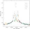 |
Fig. 1 Light curve of the lensing event KMT-2021-BLG-0322. The colors of the data points are set to match those of the telescopes used for the data acquisition. |
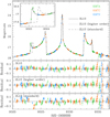 |
Fig. 2 Zoom-in view of the anomaly region of the lensing light curve. The inset in the top panel shows the enlarged view around the first peak. The solid, dotted, and dashed curves drawn over the data points are the model curves of the 3L1S, higher-order 2L1S, and standard 2L1S solutions, respectively. The three lower panels show the residuals from the individual models. The curves of the 3L1S and higher-order 2L1S models are difficult to be distinguished with the line width. |
3 Interpretations of lensing light curve
3.1 2L1S interpretation
The caustic features in the lensing light curve suggest that the event was produced by a lens composed of multiple masses. We, therefore, start with a standard 2L1S model for the interpretation of the observed lensing light curve. The modeling is done by searching for the set of the lensing parameters that best describe the observed light curve. For a 1L1S event, the lensing light curve is described by three parameters of (t0, u0, tE), which are the time of the closest lens-source approach, the separation at that time, and the event timescale, respectively. Describing a caustic-crossing 2L1S light curve requires four additional parameters of (s, q, α, ρ), which denote the separation and mass ratio between the binary lens components, M1 and M2, the angle between the source trajectory and the line connecting the binary lens components, and the ratio of the angular source radius θ* to the angular Einstein radius, that is, ρ = θ*∕θE (normalized source radius), respectively. The normalized source radius is included in modeling to account for finite-source effects during the caustic crossings of the source.
The 2L1S modeling is conducted in two steps. In the first step, we divide the lensing parameters into two groups, and the parameters s and q are searched for via a grid approach, while the other parameters are found via a downhill approach. For the downhill approach, we use the Markov Chain Monte Carlo (MCMC) algorithm. For the MCMC parameters (t0, u0, tE), the initial values are given based on the peak time, magnification, and duration of the event. For the source trajectory angle α, modeling is done with multiple starting values that are evenly divided in the 0–2π range. From the modeling in this step, weobtain a Δχ2 map on the s–q parameter plane, and identify local solutions. In the second step, we refine the local solutions identified in the first-round modeling by allowing all lensing parameters to vary. For the computations of finite-source magnifications, we use the map-making method described in Dong et al. (2006).
In Fig. 2, we present the 2L1S model curve (dashed curve plotted over the data points). The lensing parameters of the model (standard 2L1S model) are listed in Table 2. The binary lensing parameters (s, q)~ (1.1, 0.14) are similar to those of the Hirao model obtained from the modeling conducted in the early stage of the event. The lens system configuration is shown in Fig. 3, in which the caustic and the source trajectory are drawn in gray. The coordinates of the configuration are scaled to θE corresponding to the total mass of the binary lens, and the origin of the coordinates is set at the photocenter defined by Di Stefano & Mao (1996) and An & Han (2002). According to the best-fit 2L1S model, the caustic forms a single closed curve with six cusps (resonant caustic), and the source passed the left side of the caustic, passing through the caustic three times, with the individual passages producing the caustic-crossing features in the lensing light curve. Due to the resonant nature of the caustic, the solution is unique without any degeneracy.
It is found that the standard 2L1S model cannot precisely explain the observed light curve. This can be seen in the bottom panels of Fig. 2, in which we present the residuals from the 2L1S model. Although the model depicts the overall features of the light curve, there is an offset in the time of the first peak between the model and observed data (see the zoom-in view aroundthe fist caustic crossing shown in the inset inserted in the upper panel of Fig. 2). Besides the region of this peak, there exist noticeable residuals throughout the region of the caustic features. This indicates that the standard 2L1S interpretation is not adequate and a more sophisticated model is needed for the precise description of the data.
We checked the possibility that the major deviation from the 2L1S model, that is, the offset between the model and data in the region of the first peak, can be explained by higher-order effects. We considered two higher-order effects that cause the relative lens-source motion to be nonrectilinear: microlens-parallax and lens-orbital effects. The former effect is caused by the nonlinear motion of an observer caused by the Earth’s orbital motion around the Sun (Gould 1992), and the latter effect is caused by the orbital motion of the binary lens (Dominik 1998; Ioka et al. 1999). In order to check these higher-order effects, we conduct additional modeling by adding two extra pairs of parameters (πE,N, πE,E) and (d s∕dt, dα∕dt): higher-order 2L1S model.The first pair of the higher-order lensing parameters represent the north and east components of the microlens-parallax vector πE,
 (2)
(2)
respectively, and the second pair represent the annual change rates of the binary separation and source trajectory angle, respectively. Here, μrel represents the relative lens-source proper motion, 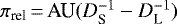 is the relative lens-source parallax, and DL and DS denote the distances to the lens and source, respectively. In this modeling, we restrict the lensing parameters to satisfy the dynamical condition of
  , where (KE/PE) and
  represent the intrinsic and projected kinetic-to-potential energy ratio, respectively (Dong et al. 2009).
We find that the residuals from the standard 2L1S model are greatly reduced with the consideration of the higher-order effects. This is shown in Fig. 2, in which we present the model curve (dotted curve) and residuals from the model. It is found that the higher-order model explains not only the major deviation in the offset of the first peak but also improves the fit throughout the anomaly region. The χ2 difference between the standard and higher-order models is Δχ2 = 2416.8. The lensing parameters of the higher-order 2L1S model are listed in Table 2. The lens system configuration of the higher-order 2L1S model is presented in Fig. 3, which shows that the caustic shape varies in time due to the lens-orbital effect and that the source trajectory becomes nonrectilinear due to the microlens-parallax effect. Figure 4 shows the Δχ2 distribution of points in the MCMC chain on the planes of higher-order parameters. It shows that these parameters are strongly correlated because the microlens-parallax and lens-orbital effects induce similar deviations in lensing light curves (Batista et al. 2011). As a result, the uncertainties of the higher-order lensing parameters are considerable, for example, πE,N = −2.31 ± 2.05 and d α∕d t = (3.57 ± 2.12) yr−1, despite the obvious effects on the lensing light curve. Also shown in Fig. 4 is the distribution of the projected kinetic-to-potential energy ratio. The mean and standard deviation of the ratio distribution are  , which is well within the range of
  for moderate eccentricity binaries that are observed at usual viewing angles.
Error bar normalization factors.
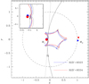 |
Fig. 3 Lens system configuration according to the 2L1S model. The concave curve represents the caustic, the line with an arrow is the source trajectory, and the filled dots marked by M1 and M2 indicate the positions of the lens components. The caustic of the standard model are drawn in gray. For the higher-order model, in which the lens position and caustic vary in time because of the lens orbital motion, we mark the lens and caustic at two epochs of HJD′ = 9323 (marked in blue color) and 9334 (in red color). The source trajectories of the standard and higher-order models are drawn in gray and black. The inset shows the zoom-in view of the region around M1. The coordinates are centered at the photocenter and lengths are scaled to the angular Einstein radius corresponding to the total mass of the lens. The dashed unit circle centered at the origin represents the Einstein ring. |
Best-fit lensing parameters of 2L1S solution.
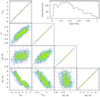 |
Fig. 4 Δχ2 distribution of points in the MCMC chain of the 2L1S solution on the planes of higher-order parameters: πE,N, πE,E, d s∕d t, and d α∕dt. Points with different colors indicate those with Δχ2 ≤ 1σ (red), ≤2σ (yellow), ≤ 3σ (green), ≤ 4σ (cyan), and ≤ 5σ (blue). The upper right panel shows the distribution of the projected kinetic-to-potential energy ratio. |
3.2 3L1S interpretation
We also test a 3L1S modeling for the interpretation of the residuals from the standard 2L1S model. In addition to the 2L1S lensing parameters, a 3L1S modeling requires extra parameters in order to describe the third lens component, M3. These parameters are (s3, q3, ψ), which denote the projected separation and mass ratio between M1 and M3, and the orientation angle of M3 as measured from the M1 –M2 axis with a center at the position of M1. Hereafter, we denote the separation and mass ratio between M1 and M2 as (s2, q2) to distinguish them from those of the third body. We check a 3L1S model because it is known that a third body of a lens can induce a small distortion of the caustic, particularly in the neighborhood of a cusp, and this may explain the deviations from the standard 2L1S model. For example, Gould et al. (2014) showed that the three parameters (s3, q3, ψ) of the planetary companion in the 3L1S event OGLE-2013-BLG-0341 could be fully recovered even when the data that were affected by the planetary caustic were eliminated from the fit, due to the distortion induced by the planet on a cusp associated with the binary-lens caustic. In particular, they argued that planets could be discovered from such cusp distortions even when the source did not passnear or over the planetary caustic.
Similar to the 2L1S modeling, the 3L1S modeling is carried out in two steps. In the first step, we conduct grid searches for the triple-lens parameters, that is, (s3, q3, ψ), by fixing the 2L1S parameters as those of the best-fit standard 2L1S model. We fix the 2L1S parameters because the 2L1S model describes the overall pattern of the light curve and the variation in the lensing lightcurve by the third body would be minor (Bozza 1999; Han et al. 2001). This step yields Δχ2 maps on the s3 –q3-ψ planes, and we identify local solutions from the maps. In the second step, the individual local solutions found from the first step are refined by allowing all parameters to vary.
Figure 5 shows the Δχ2 map on the log s3– logq3 plane obtained from the grid search. The map shows two locals at (log s3, logq3) ~ (0.1, −2.0) (wide solution) and ~ (−0.1, −2.0) (close solution). The lensing parameters of the two solutions obtained by refining these locals are listed in Table 3 (standard model) along with the χ2 values of the fits for the individual solutions. The M1 –M3 separations of the two solutions are approximately in the relation of s3,w × s3,c ~ 1.0, indicating that the degeneracy between the two solutions is caused by the close-wide degeneracy (Griest & Safizadeh 1998; Dominik 1999). Here s3,w and s3,c denote the M1 –M3 separations of the solutions with s3 > 1.0 and s3 < 1.0, respectively.It is found that the wide solution provides a better fit than the close solution with Δχ2 = 23.1, which is significant enough to resolve the degeneracy between the solutions. According to the wide 3L1S solution, the mass ratio between M1 and M3, q3 = 9.9 × 10⁻³, is very small, indicating that the third body is a planet-mass object. The projected separations of M2 and M3 from M1 for the (wide) 3L1S solution, s2 ~ 1.12 and s3 ~ 1.23, are similar to each other. According to Eq. (1) of Holman & Wiegert (1999), the maximum ratio between M3 –M1 and M2 –M1 separations for the dynamical stability of the planet is ~ 0.42 assuming a circular planet orbit. The ratio s3∕s2 ~ 1.1 is substantially greater than this critical ratio. Then, M2 should lie at a large separation along the line of sight in front of or at the back of M1 in order for the planetary system to be dynamically stable.
The model curves of the wide 3L1S model (solid curve) and the residuals from the model are shown in Fig. 2. It is found that the 3L1S model well describes all the anomaly features, significantly improving the fit, by Δχ2 = 2407, with respect to the standard 2L1S model. The fit improvement occurs not only around the region of the first peak, for which the 2L1S model exhibited a time offset between the model and data, but also throughout the whole anomaly region.
The lens system configuration of the 3L1S solutions is shown in Fig. 6: upper panel for the wide solution and lower panel for the close solution. The positions of the individual lens components are represented by red filled dots, marked by M1, M2, and M3. From the comparison of the caustic with the 2L1S caustic, drawn in gray, it is found that the tertiary lens component has two effects on the caustic. First, M3 induces a new set of caustic at around the source position of (xs, ys) ~ (0.35, −0.1) for the wide solution and ~(−0.3, −0.3) for the close solution, and this makes the caustic nested and self-intersecting. Second, M3 additionally causes a slight distortion of the caustic from that of the 2L1S solution. The source did not pass the region near the additional caustic structures induced by M3. Nevertheless, the light curve deviates from the 2L1S form due to the distortion of the caustic, and this explains the residuals from the standard 2L1S model. If the 3L1S interpretation is correct, KMT-2021-BLG-0322 is the third case in which a planet belonging to a binary is detected through the signal from the caustic distortion induced by a tertiary lens component after the cases of OGLE-2007-BLG-349 and OGLE-2013-BLG-0341.
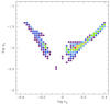 |
Fig. 5 Δχ2 map on the logs3– logq3 plane obtained from the grid search. Color coding is set to represent points with Δχ2 ≤ 1nσ (red), ≤ 2nσ (yellow), ≤ 3nσ (green), ≤ 4nσ (cyan), ≤ 5nσ (blue), ≤ 6nσ (purple), where n = 3. |
Best-fit lensing parameters of 3L1S solutions.
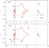 |
Fig. 6 Lens system configurations according to the wide (upper panel) and close (lower panel) 3L1S solutions. In each panel, the nested concave curve represents the caustic, the line with an arrow is the source trajectory, and the three filled red dots marked by M1, M2, and M3 indicate the positions of the lens components. The caustic curve and the source trajectory according to the static 2L1S model are drawn in gray to show the caustic variation by the third body M3. Other notations are same as those in Fig. 3. |
3.3 2L1S versus 3L1S interpretations
The analyses conducted in the previous subsections show that the deviations from a standard 2L1S model in the lensing light curve of KMT-2021-BLG-0322 can be explained almost equally well by considering the higher-order effects or by introducing a low-mass tertiary lens component. The degeneracy between the two models can be seen by comparing the residuals from the two models presented in Fig. 2. In Fig. 7, we present the cumulative distribution of 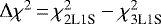 to better show the subtle difference between the fits of the two models. The distribution shows that Δχ2 ≲ 2 throughout the major anomaly region, indicating that the degeneracy between the two models is very severe.
The degeneracy between a higher-order 2L1S model and a triple-lens model for KMT-2021-BLG-0322 is very similar to the degeneraciesidentified in the two previous lensing events MACHO-97-BLG-41 and OGLE-2013-BLG-0723, for which the residuals from the standard 2L1S models were initially interpreted as signals of a planetary-mass companion to a binary lens but later explained by the higher-order effects of the 2L1S models. For these previous events, the degeneracies could be resolved because the 2L1S models yielded better fits than the corresponding 3L1S models. For KMT-2021-BLG-0322, on the other hand, the degeneracy between the two interpretations is so severe that it cannot be resolved based on only the photometry data. Therefore, KMT-2021-BLG-0322, together with the two previous events, demonstrates that the degeneracy can be not only common but also very severe.
The degeneracy also calls into question the idea from Gould et al. (2014) that it would be possible to detect planets from the distortions that they induce on the cusps. This may be possible in some cases, but at least in this case, if the planet was the real cause of the light curve discrepancy, it could not be distinguished from a nonrectilinear motion. This emphasizes the need to check both interpretations when such deviations are detected in lensing light curves.
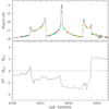 |
Fig. 7 Cumulative distribution of χ2 difference between higher-order 2L1S and 3L1S models. The light curve in the upper panel is inserted to show the region of χ2 difference. |
4 Lensing observables
Because it is difficult to single out a model for the observed data, we estimate two sets of the physical lens parameters based on the observables of the two possible interpretations of the event. The mass M and distance DL to the lens can be constrained by measuring lensing observables. The event timescale tE is the first such an observable, and it is related to M and DL by
 (3)
(3)
where κ = 4G∕(c2AU). The other two observables are the microlens parallax πE and angular Einstein radius θE, with which M and DL are uniquely determined by
 (4)
(4)
where πS = AU∕DS is the parallax to the source (Gould 2000).
The microlens parallax is measured from the slight deviation in the lensing light curve caused by the orbital motion of Earth. The microlens-parallax parameters of the 2L1S model are listed in Table 2. For the measurements of the parallax parameters corresponding to the 3L1S model, we conduct an additional modeling by considering the microlens-parallax effect, and the lensing parameters of the model including (πE,N, πE,E) are listed in Table 3. It is found that the consideration of the microlens-parallax effect improves the 3L1S fit by Δχ2 = 11.6 with respect to the standard model. The left and right panels of Fig. 8 show the Δχ2 plots of MCMC points on the πE,E–πE,N plane for the 2L1S and 3L1S solutions, respectively. For both models, it is found that the uncertainty of the north component of the microlens-parallax vector is large, while the east component is relatively well constrained.
The angular Einstein radius is measured by analyzing the deviations of the lensing light curve from a point-source form causedby finite-source effects during the caustic crossings. This analysis yields the normalized source radius ρ, and the angular Einstein radius is determined by θE = θ*∕ρ, where the angular source radius θ* is deduced from the color and brightness of the source. We estimate the extinction and reddening-corrected (dereddened) source color and brightness,  , from the instrumental values, (V − I, I), using the Yoo et al. (2004) method, in which the centroid of red giant clump (RGC) in the color-magnitude diagram (CMD) is used as a reference for this conversion. The RGC centroid can be used as a reference because its dereddened color and brightness,
  , are known, and the source and RGC stars, both of which are located in the bulge, experience similar reddening and extinction.
Figure 9 shows the source position (blue dot) with respect to the RGC centroid (red dot) in the CMD of stars around the source. The source color and magnitude are estimated from the regression of the KMTC pyDIA data to the model, and align them to the OGLE-III system to show calibrated color and magnitude values. The instrumental colors and magnitudes of the source and RGC centroid are (V − I, I) = (2.19 ± 0.02, 19.64 ± 0.01) and  , respectively.From the measured offsets in the color and magnitude between the source and RGC centroid, Δ(V − I, I), together with the known dereddened values of theRGC centroid
  (Bensby et al. 2013; Nataf et al. 2013), the dereddened source color and brightness are estimated as

 (5)
(5)
We note that the source color and brightness are estimated using the higher-order 2L1S and the 3L1S model result in consistent values. The measured V − I color is then converted into V − K color using the Bessell & Brett (1988) color relation, and we then estimate θ* from the (V − K)–θ* relation of Kervella et al. (2004). This procedure yields the angular source radius of
 (6)
(6)
With the measured angular source radius, the angular Einstein radius and the relative lens-source proper motion are determined as
 (7)
(7)
and
 (8)
(8)
respectively.
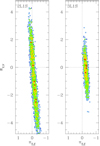 |
Fig. 8 Δχ2 distribution of points in the MCMC chain for the higher-order 2L1S (left panel) and 3L1S wide (right panel) solutions plotted on the πE,E–πE,N plane. Colorcoding is same as that of Fig. 4. |
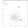 |
Fig. 9 Positions of the source with respect to the centroid of red giant clump (RGC) in the instrumental color-magnitude diagram of stars located around the source. |
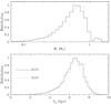 |
Fig. 10 Bayesian posteriors of the primary lens mass (M1, upper panel)and distance (lower panel) to the lens. In each panel, the solid and dotted curves represent the distributions obtained using the observables of the 2L1S and 3L1S solutions, respectively. |
5 Physical lens parameters
In this section, we estimate the physical parameters of the mass and distance to the lens by conducting a Bayesian analysis using the measured observables of (tE, θ, πE) together with the prior models of the lens mass function and the physical and dynamical distributions of Galactic objects. Because the degeneracy between the 2L1S and 3L1S solutions cannot be broken, we conduct two sets analysis based on the parameters and observables of the individual solutions.
We carry out the Bayesian analysis in two steps. In the first step, we generate a large number (6 × 10⁶) of artificial lensing events by conducting a Monte Carlo simulation, in which the mass of the lens, the distance to the lens and source, and the transverse lens-source velocity, v⊥, are deduced from the Galactic model. In the Galactic model used in the simulation, we adopt the Han & Gould (2003), Han & Gould (1995), and Zhang et al. (2020) models for the physical, dynamical distributions, and mass function, respectively.For the individual simulated events, we compute the lensing observables using the relations tE = DLθE∕v⊥,  , and πE = πrelθE. In the second step, we construct the posterior distributions of the M and DL for the artificial events with observables that are consistent with the measured values.
Figure 10 shows the posterior distributions of the primary lens mass (M1) and distance obtained from the Bayesian analysis. The distributions of the 2L1S (solid curve) and 3L1S (dotted curve) solutions are similar to each other due to the similarity of the observables between the two solutions. The estimated masses of the binary lens components are
 (9)
(9)
for both 2L1S and 3L1S solutions, indicating that the binary is composed of a K-type dwarf and a low-mass object at the star/brown-dwarf boundary. The mass of the tertiary lens component according to the 3L1S solution is
 (10)
(10)
which is in the planetary mass regime. If the 3L1S interpretation could be shown to be correct, then the planet would be the seventh microlensing planet in a binary. The system is located at a distance from Earth of
 (11)
(11)
For the estimation of M and DL, we take the median as representative values and the errors are estimated as the 16% and 84% of the distributions.
6 Conclusion
We investigated the microlensing event KMT-2021-BLG-0322, for which the lensing light curve exhibited three distinctive sets of caustic-crossing features. It was found that the overall feature of the light curve was approximately described by a binary-lens model, but the model left substantial residuals. We tested various interpretations with the aim of explaining the residuals. From this investigation, it was found that the residuals could be explained either by considering a nonrectilinear relative lens-source motion caused by the microlens-parallax and lens-orbital effects or by introducing a low-mass companion to the binary lens. The degeneracy between the higher-order 2L1S model and the triple-lens model was very severe, making it difficult to single out a correct solution based on only the photometric data. This degeneracy was known before for two previous events (MACHO-97-BLG-41 and OGLE-2013-BLG-0723), which led to the false detections of planets in binary systems. Therefore, KMT-2021-BLG-0322, together with the two previous events, demonstrates that the degeneracy can be not only common but also very severe, emphasizing the need to check both models in the interpretations of deviations from 2L1S models. From the Bayesian analysis conducted with the measured lensing observables, it was estimated that the binary lens components have masses  , for both 2L1S and 3L1S solutions, and the mass of the tertiary lens component according to the 3L1S solution is
  .
.
Acknowledgements
Work by C.H. was supported by the grants of National Research Foundation of Korea (2020R1A4A2002885 and 2019R1A2C2085965). This research has made use of the KMTNet system operated by the Korea Astronomy and Space Science Institute (KASI) and the data were obtained at three host sites of CTIO in Chile, SAAO in South Africa, and SSO in Australia. Work by I.K. was supported by JSPS KAKENHI grant number 20J20633. Work by D.P.B., A.B., and C.R. was supported by NASA through grant NASA-80NSSC18K027. T.S. acknowledges the financial support from the JSPS, JSPS23103002, JSPS24253004, and JSPS2624702. Work by N.K. is supported by JSPS KAKENHI grant number JP18J00897. The MOA project is supported by J SPS KAK-ENHI grant numbers JSPS24253004, JSPS26247023, JSPS23340064, JSPS15H00781, JP16H06287, 17H02871, and 19KK0082.
References
- Alard, C., & Lupton, R. H. 1998, ApJ, 503, 325 [Google Scholar]
- Albrow, M. 2017, https://doi.org/10.5281/zenodo.268049 [Google Scholar]
- Albrow, M. D., Beaulieu, J.-P., Caldwell, J. A. R., et al. 2000, ApJ, 534, 894 [NASA ADS] [CrossRef] [Google Scholar]
- An, J. H., & Han, C. 2002, ApJ, 573, 351 [NASA ADS] [CrossRef] [Google Scholar]
- Batista, V., Gould, A., Dieters, S., et al. 2011, A&A, 529, 102 [Google Scholar]
- Bennett, D. P., Rhie, S. H., Becker, A. C., et al. 1999, Nature, 402, 57 [NASA ADS] [CrossRef] [Google Scholar]
- Bennett, D. P., Rhie, S. H., Udalski, A., et al. 2016, AJ, 152, 125 [Google Scholar]
- Bensby, T., Yee, J. C., Feltzing, S., et al. 2013, A&A, 549, A147 [NASA ADS] [CrossRef] [EDP Sciences] [Google Scholar]
- Bessell, M. S.,& Brett, J. M. 1988, PASP, 100, 1134 [Google Scholar]
- Bond, I. A., Abe, F., Dodd, R. J., et al. 2001, MNRAS, 327, 868 [Google Scholar]
- Bozza, V. 1999, A&A, 348, 311 [NASA ADS] [Google Scholar]
- Di Stefano, R., & Mao, S. 1996, ApJ, 457, 93 [NASA ADS] [CrossRef] [Google Scholar]
- Dominik, M. 1998, A&A, 329, 361 [NASA ADS] [Google Scholar]
- Dominik, M. 1999, A&A, 349, 108 [NASA ADS] [Google Scholar]
- Dong, S., DePoy, D. L., Gaudi, B. S., et al. 2006, ApJ, 642, 842 [NASA ADS] [CrossRef] [Google Scholar]
- Dong, S., Gould, A., Udalski, A., et al. 2009, ApJ, 695, 970 [NASA ADS] [CrossRef] [Google Scholar]
- Gonzalez, O. A., Rejkuba, M., Zoccali, M., et al. 2012, A&A, 543, A13 [NASA ADS] [CrossRef] [EDP Sciences] [Google Scholar]
- Gould, A. 1992, ApJ, 392, 442 [Google Scholar]
- Gould, A. 2000, ApJ, 542, 785 [NASA ADS] [CrossRef] [Google Scholar]
- Gould, A., Udalski, A., Shin, I.-G., et al. 2014, Science, 345, 46 [Google Scholar]
- Griest, K., & Safizadeh, N. 1998, ApJ, 500, 37 [Google Scholar]
- Han, C., & Gould, A. 1995, ApJ, 447, 53 [Google Scholar]
- Han, C., & Gould, A. 2003, ApJ, 592, 172 [Google Scholar]
- Han, C., Chang, H.-Y., An, J. H., & Chang, K. 2001, MNRAS, 328, 986 [NASA ADS] [CrossRef] [Google Scholar]
- Han, C., Bennett, D. P., Udalski, A., et al. 2016, ApJ, 825, 8 [NASA ADS] [CrossRef] [Google Scholar]
- Han, C., Udalski, A., Gould, A., et al. 2017, AJ, 154, 223 [Google Scholar]
- Han, C., Lee, C.-U., Udalski, A., et al. 2020, AJ, 159, 48 [Google Scholar]
- Han, C., Udalski, A., Lee, C.-U., et al. 2021, AJ, submitted [Google Scholar]
- Holman, M. J., & Wiegert, P. A. 1999, AJ, 117, 621 [Google Scholar]
- Ioka, K., Nishi, R., & Kan-Ya, Y. 1999, Prog. Theo. Phys., 102, 98 [Google Scholar]
- Jung, Y. K., Han, C., Gould, A., et al. 2013, ApJ, 768, L7 [NASA ADS] [CrossRef] [Google Scholar]
- Kervella, P., Thévenin, F., Di Folco, E., & Ségransan, D. 2004, A&A, 426, 29 [Google Scholar]
- Kim, S.-L., Lee, C.-U., Park, B.-G., et al. 2016, JKAS, 49, 37 [Google Scholar]
- Kim, D.-J., Kim, H.-W., Hwang, K.-H., et al. 2018, AJ, 155, 76 [Google Scholar]
- Lee, D.-W., Lee, C.-U., Park, B.-G., et al. 2008, ApJ, 672, 623 [NASA ADS] [CrossRef] [Google Scholar]
- Nataf, D. M., Gould, A., Fouqué, P., et al. 2013, ApJ, 769, 88 [Google Scholar]
- Poleski, R., Skowron, J., Udalski, A., et al. 2014, ApJ, 795, 42 [Google Scholar]
- Szymański, M. K., Udalski, A., Soszyński, I., 2011, Acta Astron., 61, 83 [NASA ADS] [Google Scholar]
- Tomaney, A. B., & Crotts, A. P. S. 1996, AJ, 112, 2872 [Google Scholar]
- Udalski, A., Jung, Y. K., Han, C., et al. 2015, ApJ, 812, 47 [NASA ADS] [CrossRef] [Google Scholar]
- Yee, J. C., Shvartzvald, Y., Gal-Yam, A., et al. 2012, ApJ, 755, 102 [Google Scholar]
- Yoo, J., DePoy, D. L., Gal-Yam, A., et al. 2004, ApJ, 603, 139 [Google Scholar]
- Zang, W., Han, C., Kondo, I., et al. 2021, Res. Astron. Astrophys., in press [arXiv:2103.01896] [Google Scholar]
- Zhang, X., Zang, W., Udalski, A., et al. 2020, AJ, 159, 116 [Google Scholar]
- Zhu, W., & Dong, S. 2021, ARA&A, 59, 293 [Google Scholar]
All Tables
All Figures
|
Fig. 1 Light curve of the lensing event KMT-2021-BLG-0322. The colors of the data points are set to match those of the telescopes used for the data acquisition. |
| In the text | |
|
Fig. 2 Zoom-in view of the anomaly region of the lensing light curve. The inset in the top panel shows the enlarged view around the first peak. The solid, dotted, and dashed curves drawn over the data points are the model curves of the 3L1S, higher-order 2L1S, and standard 2L1S solutions, respectively. The three lower panels show the residuals from the individual models. The curves of the 3L1S and higher-order 2L1S models are difficult to be distinguished with the line width. |
| In the text | |
|
Fig. 3 Lens system configuration according to the 2L1S model. The concave curve represents the caustic, the line with an arrow is the source trajectory, and the filled dots marked by M1 and M2 indicate the positions of the lens components. The caustic of the standard model are drawn in gray. For the higher-order model, in which the lens position and caustic vary in time because of the lens orbital motion, we mark the lens and caustic at two epochs of HJD′ = 9323 (marked in blue color) and 9334 (in red color). The source trajectories of the standard and higher-order models are drawn in gray and black. The inset shows the zoom-in view of the region around M1. The coordinates are centered at the photocenter and lengths are scaled to the angular Einstein radius corresponding to the total mass of the lens. The dashed unit circle centered at the origin represents the Einstein ring. |
| In the text | |
|
Fig. 4 Δχ2 distribution of points in the MCMC chain of the 2L1S solution on the planes of higher-order parameters: πE,N, πE,E, d s∕d t, and d α∕dt. Points with different colors indicate those with Δχ2 ≤ 1σ (red), ≤2σ (yellow), ≤ 3σ (green), ≤ 4σ (cyan), and ≤ 5σ (blue). The upper right panel shows the distribution of the projected kinetic-to-potential energy ratio. |
| In the text | |
|
Fig. 5 Δχ2 map on the logs3– logq3 plane obtained from the grid search. Color coding is set to represent points with Δχ2 ≤ 1nσ (red), ≤ 2nσ (yellow), ≤ 3nσ (green), ≤ 4nσ (cyan), ≤ 5nσ (blue), ≤ 6nσ (purple), where n = 3. |
| In the text | |
|
Fig. 6 Lens system configurations according to the wide (upper panel) and close (lower panel) 3L1S solutions. In each panel, the nested concave curve represents the caustic, the line with an arrow is the source trajectory, and the three filled red dots marked by M1, M2, and M3 indicate the positions of the lens components. The caustic curve and the source trajectory according to the static 2L1S model are drawn in gray to show the caustic variation by the third body M3. Other notations are same as those in Fig. 3. |
| In the text | |
|
Fig. 7 Cumulative distribution of χ2 difference between higher-order 2L1S and 3L1S models. The light curve in the upper panel is inserted to show the region of χ2 difference. |
| In the text | |
|
Fig. 8 Δχ2 distribution of points in the MCMC chain for the higher-order 2L1S (left panel) and 3L1S wide (right panel) solutions plotted on the πE,E–πE,N plane. Colorcoding is same as that of Fig. 4. |
| In the text | |
|
Fig. 9 Positions of the source with respect to the centroid of red giant clump (RGC) in the instrumental color-magnitude diagram of stars located around the source. |
| In the text | |
|
Fig. 10 Bayesian posteriors of the primary lens mass (M1, upper panel)and distance (lower panel) to the lens. In each panel, the solid and dotted curves represent the distributions obtained using the observables of the 2L1S and 3L1S solutions, respectively. |
| In the text | |
Current usage metrics show cumulative count of Article Views (full-text article views including HTML views, PDF and ePub downloads, according to the available data) and Abstracts Views on Vision4Press platform.
Data correspond to usage on the plateform after 2015. The current usage metrics is available 48-96 hours after online publication and is updated daily on week days.
Initial download of the metrics may take a while.