| Issue |
A&A
Volume 655, November 2021
|
|
|---|---|---|
| Article Number | A71 | |
| Number of page(s) | 12 | |
| Section | Galactic structure, stellar clusters and populations | |
| DOI | https://doi.org/10.1051/0004-6361/202141838 | |
| Published online | 22 November 2021 | |
The impact of massive stars and black holes on the fate of open star clusters and their tidal streams
1
Department of Astronomy, School of Science, The University of Tokyo, 7-3-1 Hongo, Bunkyo-ku, Tokyo 113-0033, Japan
e-mail: long.wang@astron.s.u-tokyo.ac.jp
2
RIKEN Center for Computational Science, 7-1-26 Minatojima-minami-machi, Chuo-ku, Kobe, Hyogo 648-0047, Japan
3
European Space Agency (ESA), European Space Research and Technology Centre (ESTEC), Keplerlaan 1, 2201 AZ Noordwijk, The Netherlands
e-mail: tereza.jerabkova@es.int
Received:
21
July
2021
Accepted:
8
September
2021
Context. We use present-day observations to investigate how the content of massive OB stars affects the long-term evolution of young open clusters and their tidal streams, and how such an effect influences the constraint of initial conditions.
Aims. OB stars are typically found in binaries. They have a strong wind mass loss during the first few million years and many become black holes. These affect the dynamical evolution of an open star cluster and impact its dissolution in a given Galactic potential. We investigate the correlation between the mass of OB stars and the observational properties of open clusters. Hyades-like star clusters are well represented in the solar neighborhood and thus allow comparisons with observational data.
Methods. We perform a large number of star-by-star numerical N-body simulations of Hyades-like star clusters using the high-performance N-body code PETAR combined with GALPY.
Results. We find that OB stars and black holes have a major effect on star cluster evolution. Star clusters with the same initial conditions but a different initial content of OB stars follow very different evolutionary paths. Thus, the initial total mass and radius of an observed star cluster cannot be unambiguously determined unless the initial content of OB stars is known. We show that the stellar counts in the corresponding tidal tails, which can be identified in the Gaia data, help to resolve this issues. We thus emphasize the importance of exploring not only star clusters but also their corresponding tidal tails. These findings are relevant for studies of the formation of massive stars.
Key words: open clusters and associations: individual: Hyades / stars: formation / methods: numerical
© ESO 2021
1. Introduction
Young open star clusters are important stellar systems for understanding star formation and stellar evolution. Due to the stellar and dynamical evolution, star clusters are evaporating their stars and are in the process of becoming part of the Galactic field stellar population. Thus, for many star clusters, a large fraction of their stars are no longer located in the clusters themselves but in the large-scale tidal tails shaped by the Galactic tides and internal cluster processes (Baumgardt & Makino 2003; Heggie & Hut 2003; Chumak & Rastorguev 2006; Küpper et al. 2008, 2010; Dinnbier & Kroupa 2020a,b; Jerabkova et al. 2021).
The third data release of the Gaia survey, EDR3 (Gaia Collaboration 2021), provides rich astrometric and photometric data allowing the kinematic properties of stars in the solar neighborhood to be studied in unprecedented detail. A new era comes as increasing numbers of new open clusters (e.g., Cantat-Gaudin et al. 2018, 2019; Castro-Ginard et al. 2018, 2020; Sim et al. 2019; Liu & Pang 2019; Ferreira et al. 2020; He et al. 2021), large-scale co-eval relic filaments (Jerabkova et al. 2019; Beccari et al. 2020), and extended stellar streams (Kounkel & Covey 2019) are discovered using Gaia. With the Gaia data, for the first time, it has become possible to extract tidal tails of open star clusters, a challenging task because of the difficulty in distinguishing tail stars from the Galactic field population (e.g., Röser & Schilbach 2019; Röser et al. 2019; Fürnkranz et al. 2019; Meingast et al. 2019; Tang et al. 2019; Zhang et al. 2020; Bhattacharya et al. 2021; Jerabkova et al. 2021). The kinematic properties of Galactic young star clusters (e.g., Kuhn et al. 2019; Monteiro & Dias 2019; Monteiro et al. 2020; Zhong et al. 2020; Angelo et al. 2021; Dias et al. 2021; Godoy-Rivera et al. 2021) and their extended structures (e.g., Pang et al. 2020, 2021a; Meingast et al. 2021) have also been significantly improved.
With data on the tidal tails of open clusters becoming available, the initial conditions of these can be better constrained. These in turn constrain star formation theories and can be used to answer the following open questions: Do all stars form in initially gravitationally bound clusters? What are the radii and masses of these, and are the stellar and binary populations in these always the same? Inferring the initial conditions of star clusters constitutes an important astrophysical problem, because the observed coeval stellar population can then be matched to the physical conditions of its birth. However, star cluster formation starting from giant molecular clouds involves multi-scale complexity. The formation of a star cluster is not an isolated event, but is embedded in a large-scale distribution of molecular cloud. For example, the Orion molecular cloud has a length scale of hundreds of parsecs where several star-forming regions exist (e.g., Bally et al. 1987; Genzel & Stutzki 1989; Carpenter 2000; Dame et al. 2001; Kounkel et al. 2018; Jerabkova et al. 2019; Beccari et al. 2020).
Meanwhile, in the dense region where star clusters form, the wind, the radiation, and the supernova feedback from massive OB stars significantly affect the star formation. These phenomena can remove the gas from the cluster-forming region in a short timescale (≈1 Myr) (e.g., Kroupa et al. 2001; Goodwin & Bastian 2006; Baumgardt & Kroupa 2007; Dinnbier & Walch 2020; González-Samaniego & Vazquez-Semadeni 2020; Fujii et al. 2021b). If the star formation efficiency is low, the gas expulsion can significantly change the gravitational potential and even cause the immediate destruction of the system. The feedback can also affect the surrounding large-scale molecular cloud, such as the formation of the Orion-Eridanus Superbubble (e.g., Blaauw 1964; Brown et al. 1994; Madsen et al. 2006; O’dell et al. 1967; O’Dell et al. 2011; Ochsendorf et al. 2015; Kounkel 2020; Großschedl et al. 2021).
It is challenging to fully understand this complexity in star formation. However, during the post-gas-expulsion phase, if a star cluster is still bound, the stellar dynamics will re-virialize the cluster, resulting in a roughly spherical stellar system, as observed today. In this work, we add strength to the finding that the massive OB stars can also significantly influence the long-term dynamical evolution of the post-gas-expulsion star clusters. The wind mass loss of OB stars after gas expulsion continues to reduce the gravitational potential of the star cluster. Meanwhile, the death of OB stars can leave compact objects like black holes (BHs). By being much more massive than stars, these latter are the most likely candidates to end up in dynamically formed binaries. The interaction between these binaries and surrounding stars is a heating mechanism that influences the long-term evolution of the system (e.g., Binney & Tremaine 1987; Spitzer 1987; Mackey et al. 2008; Breen & Heggie 2013).
The number of OB stars formed is related to the fundamental nature of the initial mass function (IMF) in a star-forming region (Kroupa & Weidner 2013). If star formation were to be stochastic, the number of OB stars in a gas cloud would be described by randomly sampling the IMF. Thus, even if a group of low-mass open clusters were to have the same initial properties (i.e., the same masses and radii), they would show noticeable differences after hundreds of millions of years of dynamical evolution owing to the large variation in the number of OB stars. In contrast, if star formation were highly self-regulated, a strong correlation of the number of OB stars and the total mass of the cluster-forming gas cloud would result, and the stochastic effect would be significantly suppressed (e.g., Weidner & Kroupa 2006; Weidner et al. 2013; Kroupa & Weidner 2013; Yan et al. 2017).
By numerically modeling the evolution of Hyades-like open clusters, we can quantify the cluster bulk properties (mass and radius) as a function of time. For low-mass open star clusters, which only contain thousands of stars or fewer, the stochastic effect from the randomization of initial masses, positions, and velocities of stars cannot be ignored. The evolution of clusters, in terms of density, morphology, and the distribution of escaping stars, diverges increasingly with time due to the inherent chaotic nature of the system (Heggie 1988, 1996; Goodman et al. 1993). For a model of fixed initial mass, by allowing the IMF and the positions and velocities of stars to be randomly sampled, we study the degeneracy of initial configurations of post-gas-expulsion in expanded re-virialized Hyades-like open clusters (the most comprehensively observed) in order to constrain the maximum possible variation of such initial conditions that yield a comparable present-day configuration. The maximum variation is obtained by treating the IMF as a probabilistic distribution function rather than an optimally sampled distribution function (Kroupa & Weidner 2013). We point out for the first time that by combining the present-day properties of the open cluster (its mass, radius, and stellar population) with the population of stars in its tidal tails, the degeneracy can be broken: the post-gas-expulsion initial conditions for an observed open cluster can be inferred uniquely if the stellar population in its tidal tails is known along with its astrophysical age and bulk properties. In particular, the initial content of OB stars can be determined. Such constraints can then, in the future, be linked to the pre-gas-expulsion birth conditions by applying hydrodynamical modeling of the forming embedded cluster (e.g., Hirai et al. 2021; Fujii et al. 2021a,b).
First, in Sect. 2, we describe the numerical N-body code, PETAR, equipped with GALPY, and the initial condition for modeling the formation and evolution of a Hyades-like star cluster and its tidal stream. Then, in Sect. 3, we analyze the observational features and dynamical evolution of our models in detail. In particular, we focus on how the initial mass of OB stars affects the present-day properties of the cluster and its tidal stream. Finally, we summarize and discuss our findings in Sect. 4.
2. Method
2.1. The N-body code PETAR
In this work, we use the N-body code PETAR (Wang et al. 2020b) to perform the numerical simulations of the star clusters. PETAR is a high-performance N-body code that combines three algorithms:
-
the Barnes-Hut tree (Barnes & Hut 1986) for the long-range interactions;
-
the fourth-order Hermite integrator with block time-steps for middle-range interactions (e.g., Aarseth 2003);
-
and the slow-down algorithmic regularization method (SDAR; Wang et al. 2020a) for short-range interactions inside multiple systems, such as hyperbolic encounters, binaries, and hierarchical few-body systems.
The three algorithms are combined via the particle-tree particle-particle method (Oshino et al. 2011). The framework for developing parallel particle simulation codes (FDPS) is used to achieve a high performance with multi-process parallel computing (Iwasawa et al. 2016, 2020; Namekata et al. 2018).
Although the Barnes-Hut tree introduces an approximation of the force calculation to reduce the computational cost for the massive stellar systems with > 105 stars, PETAR can also simulate low-mass systems well when the accuracy parameters are set properly. The high performance and the low computational cost allow us to carry out a large ensemble of N-body simulations of low-mass clusters.
2.2. The stellar evolution package SSE/BSE
The recently updated version of single and binary stellar evolution packages, SSE and BSE, are used to simulate the wind mass loss, the type changes of stars, the mass transfer, and the mergers of binaries (Hurley et al. 2000, 2002; Banerjee et al. 2020). These population synthesis codes use the semi-empirical stellar wind prescriptions from Belczynski et al. (2010). For the formation of compact objects, we adopt the “rapid” supernova model for the remnant formation and material fallback from Fryer et al. (2012), along with the pulsation pair-instability supernova (Belczynski et al. 2016). We apply the solar metallicity (Z = 0.02) in this study.
2.3. The galactic potential package GALPY
The GALPY code (Bovy 2015) has been implemented as a plugin to PETAR via the C programme language interface. The PETAR-GALPY combination can simulate the formation and evolution of massive star clusters with their tidal streams in a variety of types of galactic potential (see Appendix A). In addition, we also implement the PETAR-Gaia Python tool for the data analysis and the comparison with observational data (see Appendix B).
The Python interface of GALPY provides more functions than the C interface. However, the latter has a much better computing performance. In this work, using PETAR we can efficiently generate a large amount of simulations for dynamically evolving open star clusters in the Milky-way potential. One simulation listed in Sect. 2.4 requires 7 min to 4 hours of computing time with one CPU core. The 4500 models in this study require about 4 days of computing using a desktop computer with an AMD Ryzen Threadripper 3990x CPU (64 cores).
In our models, we set up the Galactic potential using the MWPotential2014 from GALPY. This is a simplified static Galactic potential model including a bulge, a disk, and a dark-matter halo. As exactly reproducing the observed structure along the tidal stream of Hyades is not the purpose of this work, this approximated potential is sufficient for our study. The parameters of MWPotential2014 are as follows:
Bulge A power-law density profile with an exponentially cut-off
-
power-law exponent: −1.8
-
cut-off radius: 1.9 kpc
-
mass: 5 × 10⁹ M⊙
Disk Miyamoto & Nagai (1975) disk
-
scale length: 3.0 kpc
-
scale height: 280 pc
-
mass: 6.8 × 10¹⁰ M⊙
Halo NFW profile (Navarro et al. 1995)
-
scale radius: 16 kpc
-
local dark-matter density: 0.008 M⊙ pc−3
The MWPotential2014 assumes a solar distance to the Galactic center to be 8 kpc and the solar velocity to be 220 km s−1.
2.4. Initial conditions
2.4.1. The real Hyades cluster
The Hyades is the closest star cluster to the Sun, with a distance of 45 pc. Röser et al. (2011, 2019) constrained the Hyades’ half-mass and the tidal radii to be 4.1 pc and 9 pc (up to 10.4 pc), respectively. The total stellar mass of Hyades is 435 M⊙ (up to 509 M⊙) and the bound mass is 275 M⊙ (up to 322 M⊙). The upper estimated are correction based on assumptions about unresolved binaries; for more details see Röser et al. (2011). See also Reino et al. (2018) for constraints on the Hyades cluster membership and velocity dispersion and a relevant discussion in Jerabkova et al. (2021).
To find the initial position and velocity of the Hyades cluster in the Galaxy, we reverse the velocity of the center of Hyades at the present day and integrate back 648 Myr using the time-symmetric integrator in GALPY to find the initial position (see Fig. 1). We then reverse the velocity 648 Myr ago to obtain the initial velocity. As the MWPotential2014 is static, if we start from these initial coordinates and integrate forwards to the present day, we can recover the correct position and velocity with a small numerical error. The evaluated initial and the observed present-day coordinates of the Hyades in the International Celestial Reference System (ICRS) frame are listed in Table 1 (see Jerabkova et al. 2021; Gaia Collaboration 2018, for more details).
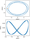 |
Fig. 1. Orbit of Hyades-like cluster in the Galactocentric reference frame calculated using GALPY. The upper panel shows the orbit in the x–y plane and the lower panel shows the orbit in the r–z plane, where r is the radial distance projected in the x–y plane. The star symbol represents the present-day position. |
Initial and present-day coordinates of Hyades.
The stellar wind mass loss and supernovae can break the conservation of the momentum. Therefore, in the N-body simulation using PETAR, the center of the star cluster may not exactly follow the orbit obtained from the result using GALPY. But the offset at the present day is small, and so it does not affect our analysis. We can also correct the offset by rotating the coordinates of the stellar system in the Galactrocentric frame1.
2.4.2. The models
Figure 2 shows a sketch describing the phase transition for the evolution of a star cluster. The gray-shaded panel shows the gas-embedded phase involving the following general steps: (i) initial convergent gas flow towards a density maximum, (ii) onset of star-formation along the filaments and predominantly at their intersection comprising the bulk of the later stellar body of the embedded star cluster, (iii) star cluster formation being affected by dynamical processes (mergers, ejections) and stellar feedback as exemplified by the Orion nebula cluster (Kroupa et al. 2018), and (iv) gas expulsion which gradually begins with the onset of star formation and results in a largely gas-free star cluster. Phases (i)–(iii) are encompassed in the birth conditions as deduced by Marks & Kroupa (2012). All of these processes contribute to the evolutionary path of the star cluster in a complex way as depicted by the bottom solid arrow pointing to the gas-free star cluster. This point marks the start of our N-body simulations, where we assume the embedded pre-gas-expulsion cluster (gray-shaded panel) has expanded and re-virialized after the residual gas has been removed (Banerjee & Kroupa 2017). Thus, we do not aim to simulate the formation of the cluster but the evolution starts from the expanded gas-free state. The long-term evolution of the star cluster and its tidal stream is controlled by the net effect of the stellar evolution, stellar dynamics, and the Galactic potential. In this work, we focus on how the content of massive stars can affect the evolution, which causes the degeneracy of the evolution track and brings the challenge of identifying the initial condition from the present-day observational properties.
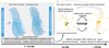 |
Fig. 2. Sketch of the formation and evolution of a star cluster (from left to right). Left: gas embedded phase where star formation occurred along the filaments in a few million years, which were influenced by the large-scale gas flow, the OB feedback, and the stellar dynamics. Right: after the gas expulsion, the bound star cluster re-virialized to a roughly spherical system, which is the initial condition in our models. With the three black solid arrows, we show that there are a number of evolutionary tracks that a star cluster can take. In our case, we focus on how the content of massive stars can affect the evolution of the cluster with otherwise identical initial conditions. We show that while this causes degeneracy, making it impossible to uniquely infer the initial conditions of an observed cluster, the properties of its tidal tails help to break the degeneracy and thus constrain the initial conditions, as marked by the gray solid arrow. The ultimate question (indicated by the gray dotted arrow) then refers to what constraints can be placed on the gas-embedded phase of the star cluster. |
Observationally, gas-free star clusters are nicely resembled by Plummer-like profiles (Plummer 1911; Röser et al. 2011; Röser & Schilbach 2019) and thus our initial setup is empirically motivated. Using the initial coordinate described in Sect. 2.4.1 in the Milky Way potential, we generate a grid of star-cluster models by varying the initial total masses M0 and the initial half-mass radii Rh, 0 (see Table 2). We combine M0 and Rh, 0, and thus the total number of model sets is 15. The reference name of each set is described in Table 2. To investigate the stochastic effect, it is necessary to carry out a large number of simulations with different random seeds. Thus, for each set, we generate 300 models by randomly sampling the IMF from Kroupa (2001) with the mass range of 0.08 − 150 M⊙ and the positions and velocities of stars from the Plummer density profile (Aarseth et al. 1974). The stochastic effect also naturally results in a different initial mass of OB stars (MOB), where we assume OB stars have a zero-age mass sequence mass of > 8 M⊙.
Initial parameters of N-body models.
3. Results
3.1. The variation of MOB due to randomly sampling the IMF
Randomly sampling the IMF results in a large dispersion in the mass of the heaviest star (mmax) and MOB model by model. Figure 3 shows the mmax − MOB relation from all 300 models in the M1600R2 set. MOB varies from 150 M⊙ to 600 M⊙ and mmax varies from 20 M⊙ to 140 M⊙. The maximum MOB comprises 37.5 per cent of the initial mass of the cluster. Thus, it is expected that the dynamical impact from the OB stars can differ significantly from model to model.
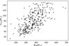 |
Fig. 3. Mass of the heaviest star (mmax) and the total mass of OB stars (MOB) by randomly sampling the Kroupa (2001) IMF in each of the 300 Hyades-like models. The initial total mass of each model is 1600 M⊙. |
3.2. The stellar winds from OB stars
To investigate how MOB affects the present-day morphology, we pick up the two models with the minimum and the maximum MOB in the M1600R2 set (hereafter named “OB-min” and “OB-max” models, respectively). Figure 4 compares the present-day positions and proper motions of stars in the ICRS frame of the two models. The OB-min model in the left panels has MOB ≈ 154 M⊙ and mmax ≈ 20 M⊙, while the OB-max model in the right panel has a much larger MOB and its mmax is comparable to the MOB of the OB-min model. Their present-day morphology looks completely different: the host star cluster still exists in the OB-min model while it has already been disrupted in the OB-max model. This suggests that MOB has a strong impact on the long-term dynamical evolution.
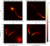 |
Fig. 4. Comparison of the number density map for the positions and proper motions of stars at the age of 648 Myr in the two models with the minimum and the maximum MOB from the M800R2 set (OB-min and OB-max models). |
The proper motions of the two branches of tidal tails also show different distributions (the upper regions of the lower panels in Fig. 4). This may be caused by the different offsets of the central position and velocity of the two models. In the OB-min model, we can correct the central coordinate to be the exact observed one, but it is difficult for the OB-max model where the center cannot be determined.
To investigate when the difference started to develop, we compare the evolution of several global parameters for the two models including the tidal radii (Rtid), the total masses inside Rtid (Mtid), the half-mass radii (Rh), and the core radii (Rc). To calculate Rc, we apply the method defined by Casertano & Hut (1985) as
where ρi is the local density of object i estimated by counting six nearest neighbors, and  is the distance to the central position of the system. The center is estimated by the density-weighted average:
where ri is the position vector of each star or compact object in the coordinate system used in the simulation. During the simulation, the origin point of the coordinate system follows the motion of the potential-weighted center of the star cluster. We highlight that the definition of Rc from observations is different. In particular, compact objects cannot be detected by observations. For massive star clusters where many BHs exist, Rc in N-body models can be very different from that of observations. In this study, only a few BHs can form and their impact on the calculation of Rc is neglectable. We have confirmed this in our models.
In the Galactic potential, there is no precise definition of Rtid, but we can obtain a rough estimation via
(Binney & Tremaine 1987), where Rgal is the distance to the Galactic center and Mgal is the effective mass of the Galaxy (the mass enclosed by Rgal). In our analysis, we first calculate the (positive) Galactic potential at the cluster center (Pgal) and then approximate Mgal via
where G is the gravitational constant. At the beginning, Mtid is unknown, and therefore the total mass of all objects is used as the starting Mtid. A few iterations are then necessary to obtain the consistent Rtid and Mtid. We stop the iteration when the difference between the new and the old Rtid is less then 1%. When the cluster reaches the disruption phase, the iteration may not converge to a positive value of Rtid, i.e., Rtid becomes zero. Once Rtid is determined, the half-mass radius (Rh) is calculated by counting all stars inside Rtid.
The comparison of these parameters for the two models is shown in Fig. 5. The difference already appears during the first 30 Myr. Rtid and Mtid of the OB-max model quickly decrease because of the strong wind mass loss of OB stars. More than half of the initial mass is lost during this period. As the gravitational potential changes, Rh and Rc of the OB-max model also increase significantly at the beginning. After approximately 400 Myr, Rh decreases while Rc significantly increases. This indicates that the star cluster loses (virial) equilibrium, and thus it rapidly expands and approaches disruption (Fukushige & Heggie 1995). This is also reflected by the oscillation of Rtid, where zero sometimes appears.
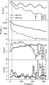 |
Fig. 5. Comparison of the evolution of the global properties for the OB-min and OB-max models shown in Fig. 4. From the top to the bottom: tidal radii (Rtid), the total masses inside Rtid (Mtid), the half-mass radii (Rh), and the core radii (Rc). The vertical line refers to 30 Myr. |
In contrast, the OB-min model has a smooth evolution and the star cluster still survives at 648 Myr with more than half of the initial mass being inside Rtid. The evolution of Rh and Rc is flat until 648 Myr.
3.3. The general trend depending on MOB
The OB-min and OB-max are two specific cases. To investigate the general trend, we separate the 300 models in each model set into five bins of MOB. Each bin contains the same number of models (60). Then, for each model in the bin, we obtain Rtid and Mtid at 648 Myr and the average values of Rh and Rc from the snapshots at 632, 640, and 648 Myr. The average can reduce the fluctuation that appears in the evolution of Rh and Rc as shown in Fig. 5. Finally, we calculate the statistic average and the standard deviation of each parameter (including MOB) inside each bin. The result is shown in Fig. 6. There is a pronounced trend in that a larger MOB results in smaller Rtid and Mtid (faster mass loss).
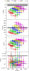 |
Fig. 6. Comparison of the evolution of the global properties for all models with different M0 (represented by colors) and different Rh, 0 (represented by markers and brightness of colors). From the top to the bottom: Rtid, Mtid, Rh, and Rc. The 300 models in each set are collected into bins of MOB. The error bars represent the standard deviation. The observed values of Hyades are shown as horizontal lines or regions (with uncertainties). |
The reference data from Hyades are shown as gray horizontal lines and regions (with uncertainties). Most of models have slightly lower Rtid, Rh, and Rc compared to those of the observational data. There is a degeneracy between MOB and M0 that many combinations of the two parameters can result in similar present-day properties of the star cluster. For example, all five M0 sets (different colors) can result in the same Rtid (4 − 8 pc), Mtid (100 − 300 M⊙), Rh (2 − 3 pc), and Rc (1 − 2 pc). This suggests that it is hard to determine the initial condition by only checking these four parameters.
The impact of Rh, 0 is not significant. Generally, smaller Rh, 0 result in larger Rtid (Mtid), but the scatter is large and the effect is less than that found for M0 and MOB.
3.4. The long-term dynamical impact from black hole binaries
The major impact from stellar wind mass loss of OB stars appears in the first 32 Myr as shown in Fig. 5. Thus, if a model has a different initial condition but shows similar properties (e.g., mass, density and Rh) at 32 Myr to those in the OB-max model, it may have identical evolution after that. To investigate this, we measured the difference between models as
where Nrh is the number of stars within Rh and the suffix “ref” refers to the parameters of the OB-max model. The values of Mtid at 32 Myr are used for comparison. Rh and Mrh fluctuate significantly, as shown in Fig. 5. We therefore compared their average values at 24, 32, and 40 Myr.
Baumgardt & Makino (2003) showed that the dissolution time of a star cluster depends the strength of tidal field (Rtid/Rh) and the relaxation time. The formula of the half-mass relaxation time for one component system can be described as (Spitzer 1987)
where Λ = 0.02N, m is the mass of the star (we use the average mass instead) and G is the gravitational constant. The factor of 0.02 follows the measurement from Giersz & Heggie (1996). The three parameters in Eq. (5) can reflect the tidal effect and Trh.
We selected the models with the first five smallest Δ for each M0 set. Figure 7 shows the comparison of the dynamical evolution of these models. The models with a larger common M0 tend to have a more divergent long-term evolution. For the M800 set, all models except one show identical evolution, while the M1600 models show large differences in Rtid and Mtid after 200 Myr. Some M1600 models are still bound at 648 Myr while others have been disrupted. Such a trend depending on M0 suggests that the stellar wind mass loss at the beginning is not the only reason for the divergent evolution seen for example in the OB-min and OB-max models.
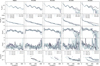 |
Fig. 7. Evolution of the global properties. From the top to bottom: Rtid, Mtid, Rh, Rc, and aBBH, for the models with similar properties at 32 Myr to those in the OB-max model. The columns separate the models with different M0. For each M0, a brighter color indicates a higher total mass of BHs (MBH). The half-mass relaxation times (Trh) at 32 Myr are shown in the second row of panels. The values of MBH and the corresponding numbers of BHs (in brackets) are shown in the last row of panels. |
The values of Trh are shown in the second row of panels in Fig. 7. Generally, models with a short Trh lose mass faster, but this is not the case for the two models in the M1600 set with Trh = 231.9 Myr and 255.4 Myr (hereafter named R1 and R2 models, respectively). The R2 model has a large Trh but dissolves faster. In the meantime, some models in the M1600 set have larger Trh than those of the M800 set, but the former have already been disrupted at the present day while the latter still survive. Thus, the different evolution cannot be explained by Trh.
Instead, we find that the existence of BH binaries (BBHs) plays an important role. The total masses (MBH), the number of BHs at 32 Myr, and the evolution of the semi-major axes of BBHs are shown in the bottom panels of Fig. 7. The R2 model in the M1600 set has four BHs with MBH = 36 M⊙ while the R1 model has no BHs. This can explain why the R2 model loses mass faster. The decrease in aBBH is found in all models with BBHs in Fig. 7, which indicates the dynamical effect of binary heating (e.g., Binney & Tremaine 1987; Spitzer 1987; Mackey et al. 2008; Breen & Heggie 2013; Wang 2020). When light stars have close encounters with the BBH, they gain significant kinetic energy and are easily kicked out from the center of a star cluster while the separation of the BBH shrinks. Such a process can drive the expansion of the stellar halo and can speed up the dissolution of the cluster. Thus, a star cluster containing more massive BBHs tends to lose mass faster. In summary, MOB not only affects the strength of stellar wind at the early phase of the star cluster, but also influences the formation of BBHs and the long-term evolution of the system.
3.5. The structure of tidal streams
It is difficult to reconstruct the initial condition from the present-day property of a star cluster because of the random value of MOB. However, the tidal stream, which records the history of escapers, may provide an additional constraint. To investigate this, we selected the OB-min model in the M800R2 set as the reference, and then, for each M0, we found the most similar model with the minimum Δ at the present day. Five models with different M0 were collected.
The morphology, the number density distribution, and the average mass distribution of these (five) models at the present day are shown in Fig. 8. For a better comparison, we correct the central position of each model to be located at the observed position of the Hyades. The morphology (density map) is shown in the Galactocentric reference frame with the spherical coordinate system. In the longitude–latitude plot, the stream distributes in a regular shape. Thus, it is easy to count the number of stars along the stream (the longitude) and to detect substructures such as the overdensity generated by the epicyclic motion (Küpper et al. 2008).
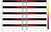 |
Fig. 8. Comparison of the morphology, density, and average mass of stars for the five models with different M0 and the minimum Δ referring to the OB-min model in the M800R2 set. For each model, the three panels show the number density map of stars in the spherical coordinate system of the Galactocentric reference frame, the histogram of star counting (Ns), and the average mass of stars (⟨ms⟩) along the longitude, respectively. The compacted objects (WDs, NSs, and BHs) are excluded. |
For all models, the lengths of the streams are similar, and the overdensities appear at 179 deg and 181 deg along the longitude. Küpper et al. (2008) showed that for a point-mass potential with a circular orbit, the distance of the overdensity to the center can be described as
where κ and Ω are epicyclic and circular frequencies, respectively. Based on the observational data of the solar neighborhood, κ/Ω ≈ 1.35 (Binney & Tremaine 1987). Thus, Rden ≈ 3.54πRtid. Since Rtid evolves, we roughly estimate the range of Rden (the gray region in Fig. 8) using the minimum and the maximum values of Rtid during the simulation. To calculate the longitude of Rden, Rgal is needed. From Fig. 1, Rgal varies between 7 and 9 kpc. We simply use the present-day value to obtain a rough estimation. The predicted positions of the overdensities are consistent with those of the models. As Rden is independent of M0, the morphology of the tidal streams does not show a pronounced difference.
We also analyzed the average mass (⟨ms⟩) along the longitude. There is a clear sign of mass segregation: ⟨ms⟩ is much larger inside the star cluster compared to that along the stream. However, there is also no pronounced difference depending on M0.
Although the structures and the mass functions of the five tidal streams are similar, we find that the star counts inside and outside Rtid strongly depend on M0. Table 3 lists the total masses and the numbers of stars with apparent G-band magnitudes < 20 inside and outside Rtid for these five models, respectively. All models have a similar Mtid and Ntid while the low-M0 model has a small Mout and Nout. As the high-M0 model has a large MOB, the dissolution of the star cluster is faster because of stronger stellar wind mass loss and dynamical heating from BBHs. Thus, the fraction of the number of stars inside Rtid (ftid = Ntid/N where N is the total number of stars) can help to estimate M0 and MOB for an observed star cluster.
From the Gaia EDR3 catalogue, 862 objects with a similar magnitude cutoff were detected, 293 of which belong to the leading tail and 166 to the trailing tail. All Nout in Table 3 are significantly higher than the observed counts. However, it is difficult to form any robust conclusion based on the direct comparison of the N-body model to the observation. For Gaia data, a strict selection is needed to remove contamination and obtain signal in the tails, which affects completeness. With a looser constraint, the contamination is higher. In addition, an unresolved binary is counted as one object and a large fraction of these are filtered out by quality cuts applied to the Gaia data (Jerabkova et al. 2021). Because of the overlap of objects along the line of sight and a higher fraction of binaries inside the star cluster, the numbers of stars might be underestimated. Meanwhile, the background contamination is expected to be higher along the tails. A better solution is to use the N-body model as the reference to create mock observations considering the Gaia uncertainty and background contamination and then to compare the model with the observation to obtain a better constraint. For such a purpose, the assumption of primordial binaries is also necessary. This is where our efforts will be concentrated in the future.
This result suggests that one strategy in particular is able to constrain the initial condition of a star cluster. First, we find a group of models with different M0 and MOB that can result in the same Rtid, Mtid, and Rh. We then use ftid to determine which combination of M0 and MOB best fits the observational data. Because of the high performance of PETAR, it is almost possible to generate a grid of star cluster models to achieve this goal.
4. Discussion and conclusion
In this work, we investigate how the content of OB stars affects the long-term evolution of Hyades-like open star clusters and their tidal streams. The models are designed to have identical initial conditions, including the shape of the IMF and the density profile. The random number of OB stars can result in a significantly different dynamical evolution of the system. As the example in Fig. 4 shows, the OB-min model with a small MOB can survive as a star cluster until the present day, while the OB-max model with a large MOB has already dissolved 200 Myr ago.
The stellar wind mass loss of OB stars during the first 32 Myr and the BBH dynamical heating both accelerate the mass loss of star clusters (Fig. 7) and cause the difference. Thus, assuming that the stochastic variation of MOB is the correct physical model, it is not possible to constrain the initial condition (e.g., M0 and MOB) of an observed star cluster confidently by only checking the present-day properties inside Rtid (e.g., Mtid, Rh, and Rc). Meanwhile, we find that the morphology (overdensity) and average mass distribution along the tidal streams are independent of M0 (see Fig. 8). However, the star counts inside and outside Rtid (ftid; Table 3) can help to remove the degeneracy and help to constrain the initial condition.
There are a few aspects that are not included in our analysis. We did not consider the influence from the uncertainty on the ages in the observation. We expect that the age may affect the determination of M0 using ftid, but it may also influence the length of the tidal stream and the position of the overdensity. Thus, we may disentangle the impacts from the age and the MOB.
There are no primordial binaries in our models. Observations have shown that massive stars in open clusters are most likely all in multiple systems (Sana et al. 2012; Duchêne & Kraus 2013; Moe & Di Stefano 2017). The dynamical interactions of these multiple systems can result in ejections and mergers (e.g., Wang et al. 2019). As a result, the numbers of retained OB stars and formed BHs decrease. In addition, the primordial binaries can also provide the binary heating in the early phase that affects the timescale of core collapse (e.g., Heggie et al. 2006). All of these subsequently affect the long-term dynamical evolution of clusters. In future work, we will also consider the impact of primordial binaries.
The gas expulsion process can also significantly affect the dynamics of the star cluster during the gas embedded phase (e.g., Wang et al. 2019; Fujii et al. 2021a,b; Pang et al. 2021b) and the formation of tidal streams (Dinnbier & Kroupa 2020a,b). Ultraviolet radiation, stellar winds, and supernovae from OB stars can all drive gas expulsion. Thus, the gas expulsion is also sensitive to the stochastic nature of MOB. Stronger feedback because of more OB stars may quench the star formation earlier, and thus the star formation efficiency becomes lower. As a result, the damage to the stellar system is also stronger and a larger number of escapers are expected to appear during the first few million years. By considering gas expulsion, we expect an even larger scatter of the evolution tracks due to the variation of MOB.
As a caveat it is noted that we applied a simple Milky Way potential (MWPotential2014). There is no time-dependent evolution of the potential, no bar, and no spiral arm. As we are not aiming to obtain the precise morphology of the tidal stream for the Hyades, missing these components does not significantly influence the major conclusion. As GALPY provides support in building up a more realistic Galactic potential, we will investigate such an effect in future work.
We assumed in this work that the formation of OB stars is purely statistical, implying a large variation in MOB. But if star formation has some degree of self-regulation such that the total number and mass of OB stars depends on the initial mass of the cluster-forming gas cloud, the scatter of MOB should be much smaller than that found here. If this were the case, then constraining the initial conditions of an observed open cluster would then be much easier. For example, if the star formation is highly self-regulated such that the stars formed can be described by optimally sampling the IMF (Kroupa & Weidner 2013), MOB ≈ 289.81 M⊙ and mmax ≈ 53 M⊙ for M0 = 1600 M⊙ and only a very small scatter of MOB is allowed. Therefore, by invoking stochastic sampling from the IMF, our work provides the upper limit on the uncertainty in constraining the initial conditions of a given open star cluster.
Based on COORDINATES.BASECOORDINATEFRAME from the ASTROPY Python module (see Astropy Collaboration 2013, 2018).
GitHub page: https://github.com/lwang-astro/PeTar
Acknowledgments
L. W. thanks the financial support from JSPS International Research Fellow (School of Science, The university of Tokyo). We thank Jo Bovy for the help on the implementation of GALPY interface in PETAR and Qi Shu for the help on the debugging of the code. T. J. acknowledges support through the European Space Agency fellowship programme.
References
- Aarseth, S. J. 2003, Gravitational N-Body Simulations (Cambridge University Press) [Google Scholar]
- Aarseth, S. J., Henon, M., & Wielen, R. 1974, A&A, 37, 183 [NASA ADS] [Google Scholar]
- Angelo, M. S., Corradi, W. J. B., Santos, J. F. C., et al. 2021, MNRAS, 500, 4338 [Google Scholar]
- Astropy Collaboration (Robitaille, T. P., et al.) 2013, A&A, 558, A33 [NASA ADS] [CrossRef] [EDP Sciences] [Google Scholar]
- Astropy Collaboration (Price-Whelan, A. M., et al.) 2018, AJ, 156, 123 [Google Scholar]
- Bally, J., Langer, W. D., Stark, A. A., et al. 1987, ApJ, 312, L45 [NASA ADS] [CrossRef] [Google Scholar]
- Banerjee, S., & Kroupa, P. 2017, A&A, 597, A28 [NASA ADS] [CrossRef] [EDP Sciences] [Google Scholar]
- Banerjee, S., Belczynski, K., Fryer, C. L., et al. 2020, A&A, 639, A41 [NASA ADS] [CrossRef] [EDP Sciences] [Google Scholar]
- Baumgardt, H., & Kroupa, P. 2007, MNRAS, 380, 1589 [NASA ADS] [CrossRef] [Google Scholar]
- Baumgardt, H., & Makino, J. 2003, MNRAS, 340, 227 [NASA ADS] [CrossRef] [Google Scholar]
- Barnes, J., & Hut, P. 1986, Nature, 324, 446 [NASA ADS] [CrossRef] [Google Scholar]
- Beccari, G., Boffin, H. M. J., & Jerabkova, T. 2020, MNRAS, 491, 2205 [Google Scholar]
- Belczynski, K., Bulik, T., Fryer, C. L., et al. 2010, ApJ, 714, 1217 [NASA ADS] [CrossRef] [Google Scholar]
- Belczynski, K., Heger, A., Gladysz, W., et al. 2016, A&A, 594, A97 [NASA ADS] [CrossRef] [EDP Sciences] [Google Scholar]
- Bhattacharya, S., Agarwal, M., Rao, K. K., et al. 2021, MNRAS, 505, 1607 [NASA ADS] [CrossRef] [Google Scholar]
- Binney, J., & Tremaine, S. 1987, Galactic dynamics (Princeton, NJ: Princeton University Press) [Google Scholar]
- Blaauw, A. 1964, ARA&A, 2, 213 [Google Scholar]
- Bovy, J. 2015, ApJS, 216, 29 [NASA ADS] [CrossRef] [Google Scholar]
- Brown, A. G. A., de Geus, E. J., & de Zeeuw, P. T. 1994, A&A, 289, 101 [NASA ADS] [Google Scholar]
- Breen, P. G., & Heggie, D. C. 2013, MNRAS, 432, 2779 [NASA ADS] [CrossRef] [Google Scholar]
- Cantat-Gaudin, T., Jordi, C., Vallenari, A., et al. 2018, A&A, 618, A93 [NASA ADS] [CrossRef] [EDP Sciences] [Google Scholar]
- Cantat-Gaudin, T., Krone-Martins, A., Sedaghat, N., et al. 2019, A&A, 624, A126 [NASA ADS] [CrossRef] [EDP Sciences] [Google Scholar]
- Carpenter, J. M. 2000, AJ, 120, 3139 [Google Scholar]
- Casertano, S., & Hut, P. 1985, ApJ, 298, 80 [Google Scholar]
- Castro-Ginard, A., Jordi, C., Luri, X., et al. 2018, A&A, 618, A59 [NASA ADS] [CrossRef] [EDP Sciences] [Google Scholar]
- Castro-Ginard, A., Jordi, C., Luri, X., et al. 2020, A&A, 635, A45 [NASA ADS] [CrossRef] [EDP Sciences] [Google Scholar]
- Chumak, Y. O., & Rastorguev, A. S. 2006, Astron. Lett., 32, 157 [NASA ADS] [CrossRef] [Google Scholar]
- Dame, T. M., Hartmann, D., & Thaddeus, P. 2001, ApJ, 547, 792 [Google Scholar]
- de Bruijne, J. H. J. 1999, MNRAS, 306, 381 [Google Scholar]
- Dias, W. S., Monteiro, H., Moitinho, A., et al. 2021, MNRAS, 504, 356 [NASA ADS] [CrossRef] [Google Scholar]
- Dinnbier, F., & Kroupa, P. 2020a, A&A, 640, A84 [EDP Sciences] [Google Scholar]
- Dinnbier, F., & Kroupa, P. 2020b, A&A, 640, A85 [EDP Sciences] [Google Scholar]
- Dinnbier, F., & Walch, S. 2020, MNRAS, 499, 748 [Google Scholar]
- Duchêne, G., & Kraus, A. 2013, ARA&A, 51, 269 [Google Scholar]
- Ferreira, F. A., Corradi, W. J. B., Maia, F. F. S., et al. 2020, MNRAS, 496, 2021 [NASA ADS] [CrossRef] [Google Scholar]
- Fryer, C. L., Belczynski, K., Wiktorowicz, G., et al. 2012, ApJ, 749, 91 [Google Scholar]
- Fujii, M. S., Saitoh, T. R., Hirai, Y., et al. 2021a, PASJ, 73, 1074 [NASA ADS] [CrossRef] [Google Scholar]
- Fujii, M. S., Saitoh, T. R., Wang, L., et al. 2021b, PASJ, 73, 1057 [NASA ADS] [CrossRef] [Google Scholar]
- Fukushige, T., & Heggie, D. C. 1995, MNRAS, 276, 206 [NASA ADS] [Google Scholar]
- Fürnkranz, V., Meingast, S., & Alves, J. 2019, A&A, 624, L11 [NASA ADS] [CrossRef] [EDP Sciences] [Google Scholar]
- Gaia Collaboration (Babusiaux, C., et al.) 2018, A&A, 616, A10 [NASA ADS] [CrossRef] [EDP Sciences] [Google Scholar]
- Gaia Collaboration (Brown, A. G. A., et al.) 2021, A&A, 649, A1 [NASA ADS] [CrossRef] [EDP Sciences] [Google Scholar]
- Genzel, R., & Stutzki, J. 1989, ARA&A, 27, 41 [NASA ADS] [CrossRef] [Google Scholar]
- Giersz, M., & Heggie, D. C. 1996, MNRAS, 279, 1037 [NASA ADS] [Google Scholar]
- Godoy-Rivera, D., Pinsonneault, M. H., & Rebull, L. M. 2021, ApJS, submitted [arXiv:2101.01183] [Google Scholar]
- González-Samaniego, A., & Vazquez-Semadeni, E. 2020, MNRAS, 499, 668 [CrossRef] [Google Scholar]
- Goodman, J., Heggie, D. C., & Hut, P. 1993, ApJ, 415, 715 [Google Scholar]
- Goodwin, S. P., & Bastian, N. 2006, MNRAS, 373, 752 [Google Scholar]
- Großschedl, J. E., Alves, J., Meingast, S., et al. 2021, A&A, 647, A91 [NASA ADS] [CrossRef] [EDP Sciences] [Google Scholar]
- He, Z.-H., Xu, Y., Hao, C.-J., et al. 2021, Res. Astron. Astrophys., 21, 093 [Google Scholar]
- Heggie, D. C. 1988, NATO Advanced Study Institute on Long-Term Dynamical Behaviour of Natural and Artificial N-Body Systems, 329 [CrossRef] [Google Scholar]
- Heggie, D. C. 1996, IAUS, 174, 131 [NASA ADS] [Google Scholar]
- Heggie, D., & Hut, P. 2003, The Gravitational Million-Body Problem: A Multidisciplinary Approach to Star Cluster Dynamics (Cambridge University Press) [Google Scholar]
- Heggie, D. C., Trenti, M., & Hut, P. 2006, MNRAS, 368, 677 [CrossRef] [Google Scholar]
- Hirai, Y., Fujii, M. S., & Saitoh, T. R. 2021, PASJ, 73, 1036 [NASA ADS] [CrossRef] [Google Scholar]
- Hurley, J. R., Pols, O. R., & Tout, C. A. 2000, MNRAS, 315, 543 [Google Scholar]
- Hurley, J. R., Tout, C. A., & Pols, O. R. 2002, MNRAS, 329, 897 [Google Scholar]
- Iwasawa, M., Tanikawa, A., Hosono, N., et al. 2016, PASJ, 68, 54 [NASA ADS] [CrossRef] [Google Scholar]
- Iwasawa, M., Namekata, D., Nitadori, K., et al. 2020, PASJ, 72, 13 [CrossRef] [Google Scholar]
- Jerabkova, T., Boffin, H. M. J., Beccari, G., et al. 2019, MNRAS, 489, 4418 [NASA ADS] [CrossRef] [Google Scholar]
- Jerabkova, T., Boffin, H. M. J., Beccari, G., et al. 2021, A&A, 647, A137 [NASA ADS] [CrossRef] [EDP Sciences] [Google Scholar]
- Kroupa, P. 2001, MNRAS, 322, 231 [NASA ADS] [CrossRef] [Google Scholar]
- Kounkel, M. 2020, ApJ, 902, 122 [NASA ADS] [CrossRef] [Google Scholar]
- Kounkel, M., & Covey, K. 2019, AJ, 158, 122 [Google Scholar]
- Kounkel, M., Covey, K., Suárez, G., et al. 2018, AJ, 156, 84 [NASA ADS] [CrossRef] [Google Scholar]
- Kroupa, P., & Weidner, C. 2013, pss5.book, 115 [Google Scholar]
- Kroupa, P., Aarseth, S., & Hurley, J. 2001, MNRAS, 321, 699 [NASA ADS] [CrossRef] [Google Scholar]
- Kroupa, P., Jeřábková, T., Dinnbier, F., Beccari, G., & Yan, Z. 2018, A&A, 612, A74 [NASA ADS] [CrossRef] [EDP Sciences] [Google Scholar]
- Kuhn, M. A., Hillenbrand, L. A., Sills, A., et al. 2019, ApJ, 870, 32 [Google Scholar]
- Küpper, A. H. W., MacLeod, A., & Heggie, D. C. 2008, MNRAS, 387, 1248 [Google Scholar]
- Küpper, A. H. W., Kroupa, P., Baumgardt, H., & Heggie, D. C. 2010, MNRAS, 401, 105 [Google Scholar]
- Liu, L., & Pang, X. 2019, ApJS, 245, 32 [NASA ADS] [CrossRef] [Google Scholar]
- Mackey, A. D., Wilkinson, M. I., Davies, M. B., & Gilmore, G. F. 2008, MNRAS, 386, 65 [NASA ADS] [CrossRef] [Google Scholar]
- Madsen, G. J., Reynolds, R. J., & Haffner, L. M. 2006, ApJ, 652, 401 [CrossRef] [Google Scholar]
- Marks, M., & Kroupa, P. 2012, A&A, 543, A8 [NASA ADS] [CrossRef] [EDP Sciences] [Google Scholar]
- Meingast, S., Alves, J., & Fürnkranz, V. 2019, A&A, 622, L13 [NASA ADS] [CrossRef] [EDP Sciences] [Google Scholar]
- Meingast, S., Alves, J., & Rottensteiner, A. 2021, A&A, 645, A84 [NASA ADS] [CrossRef] [EDP Sciences] [Google Scholar]
- Miyamoto, M., & Nagai, R. 1975, PASJ, 27, 533 [NASA ADS] [Google Scholar]
- Moe, M., & Di Stefano, R. 2017, ApJS, 230, 15 [Google Scholar]
- Monteiro, H., & Dias, W. S. 2019, MNRAS, 487, 2385 [Google Scholar]
- Monteiro, H., Dias, W. S., Moitinho, A., et al. 2020, MNRAS, 499, 1874 [NASA ADS] [CrossRef] [Google Scholar]
- Namekata, D., Iwasawa, M., Nitadori, K., et al. 2018, PASJ, 70, 70 [NASA ADS] [CrossRef] [Google Scholar]
- Navarro, J. F., Frenk, C. S., & White, S. D. M. 1995, MNRAS, 275, 720 [NASA ADS] [CrossRef] [Google Scholar]
- Ochsendorf, B. B., Brown, A. G. A., Bally, J., et al. 2015, ApJ, 808, 111 [NASA ADS] [CrossRef] [Google Scholar]
- O’dell, C. R., York, D. G., Henize, K. G., et al. 1967, ApJ, 150, 835 [CrossRef] [Google Scholar]
- O’Dell, C. R., Ferland, G. J., Porter, R. L., et al. 2011, ApJ, 733, 9 [CrossRef] [Google Scholar]
- Oshino, S., Funato, Y., & Makino, J. 2011, PASJ, 63, 881 [NASA ADS] [Google Scholar]
- Pang, X., Li, Y., Tang, S.-Y., Pasquato, M., & Kouwenhoven, M. B. N. 2020, ApJ, 900, L4 [NASA ADS] [CrossRef] [Google Scholar]
- Pang, X., Li, Y., Yu, Z., et al. 2021a, ApJ, 912, 162 [NASA ADS] [CrossRef] [Google Scholar]
- Pang, X., Yu, Z., Tang, S. Y., et al. 2021b, ApJ, submitted [arXiv:2106.07658] [Google Scholar]
- Plummer, H. C. 1911, MNRAS, 71, 460 [Google Scholar]
- Reino, S., de Bruijne, J., Zari, E., et al. 2018, MNRAS, 477, 3197 [NASA ADS] [CrossRef] [Google Scholar]
- Röser, S., & Schilbach, E. 2019, A&A, 627, A4 [NASA ADS] [CrossRef] [EDP Sciences] [Google Scholar]
- Röser, S., Schilbach, E., Piskunov, A. E., Kharchenko, N. V., & Scholz, R.-D. 2011, A&A, 531, A92 [NASA ADS] [CrossRef] [EDP Sciences] [Google Scholar]
- Röser, S., Schilbach, E., & Goldman, B. 2019, A&A, 621, L2 [NASA ADS] [CrossRef] [EDP Sciences] [Google Scholar]
- Sana, H., de Mink, S. E., de Koter, A., et al. 2012, Science, 337, 444 [Google Scholar]
- Sim, G., Lee, S. H., Ann, H. B., et al. 2019, J. Korean Astron. Soc., 52, 145 [NASA ADS] [Google Scholar]
- Spitzer, L. 1987, Dynamical Evolution of Globular Clusters (Princeton University Press) [Google Scholar]
- Strömberg, G. 1939, Popular Astron., 47, 172 [Google Scholar]
- Tang, S.-Y., Pang, X., Yuan, Z., et al. 2019, ApJ, 877, 12 [Google Scholar]
- van Leeuwen, F. 2009, A&A, 497, 209 [CrossRef] [EDP Sciences] [Google Scholar]
- Wang, L. 2020, MNRAS, 491, 2413 [NASA ADS] [Google Scholar]
- Wang, L., Kroupa, P., & Jerabkova, T. 2019, MNRAS, 484, 1843 [NASA ADS] [CrossRef] [Google Scholar]
- Wang, L., Nitadori, K., & Makino, J. 2020a, MNRAS, 493, 3398 [NASA ADS] [CrossRef] [Google Scholar]
- Wang, L., Iwasawa, M., Nitadori, K., & Makino, J. 2020b, MNRAS, 497, 536 [NASA ADS] [CrossRef] [Google Scholar]
- Weidner, C., & Kroupa, P. 2006, MNRAS, 365, 1333 [Google Scholar]
- Weidner, C., Kroupa, P., & Pflamm-Altenburg, J. 2013, MNRAS, 434, 84 [NASA ADS] [CrossRef] [Google Scholar]
- Yan, Z., Jerabkova, T., & Kroupa, P. 2017, A&A, 607, A126 [NASA ADS] [CrossRef] [EDP Sciences] [Google Scholar]
- Zhang, Y., Tang, S.-Y., Chen, W. P., et al. 2020, ApJ, 889, 99 [NASA ADS] [CrossRef] [Google Scholar]
- Zhong, J., Chen, L., Wu, D., Li, L., Bai, L., & Hou, J. 2020, A&A, 640, A127 [NASA ADS] [CrossRef] [EDP Sciences] [Google Scholar]
Appendix A: PETAR - GALPY
GALPY (Bovy 2015) is state-of-the-art code for modeling the orbits of stars in different kinds of galactic potentials. The online document provides rich information about the use of the code2. The code is written mainly in the Python programme language, but C is used for coupling to the N-body codes with a high computing performance. An interface has been implemented in PETAR so that it is possible to trace the formation and evolution of tidal streams. Table A.1 lists all names of GALPY potentials (version 1.7.0) that can be accessed by PETAR. The MWPotential and MWPotential2014 are wrapped potentials (see Bovy 2015). The PETAR.GALPY.HELP tool provides the basic description of each potential type. It is recommended to use the Python interface of GALPY to configure the potential, and then to save the parameters and use PETAR to read them to initialize the potential in N-body simulations.
Supported potentials in the PETAR-GALPY interface
When GALPY is switched on, PETAR uses the Galactic center as the reference frame without rotation. To keep the high digital precision for positions and velocities of stars, the coordinate origin of the stellar system is not the Galactic center but follows the motion of the center of the cluster. The position and velocity of center referring to the Galactic center are saved as the offset values in the header of the snapshots. Using these offset values, users can easily obtain the coordinate frame referring to the Galactic center. The default way to determine the center is to use the long-range potential-weighted average of positions and velocities of all objects. This may not be the best way. It is challenging to determine the center when the star cluster is close to the complete disruption. Therefore, users may need to redetermine the center in the late phase of the evolution by using the snapshots.
The PETAR-GALPY interface allows two types of potentials to be added: the co-moving potentials and the fixed central potentials. The former co-moves with the center of the stellar system. The latter has a fixed position referring to the Galactic center. Either type can combine arbitrary time-dependent potentials listed in Table A.1. Thus, it is flexible and can be used to study a variety topics. For example, users can set up a star cluster move in the Milky Way potential with a gas halo or a dark matter halo surrounding the cluster. The gas potential can be reduced by time to represent the gas expulsion. The details needed to set up the potentials can be found in the online README of PETAR3 and from the commander ‘petar -h’.
Appendix B: Comparison with observation
To construct a bridge to connect the N-body simulations and observations, we implemented a group of data analysis tools written in Python3 (see online manual for details), Here we briefly describe the functions of these tools.
B.1. The transformation of reference frames and coordinate systems
PETAR equipped with GALPY uses the Galactocentric reference frame and the Cartesian coordinate system in the simulation. The result cannot be directly compared with the observational data. The PETAR data analysis tool includes an interface to transform the snapshot from a N-body simulation to the data type of ASTROPY.COORDINATES.SKYCOORD (Astropy Collaboration 2013, 2018). SKYCOORD is a flexible data type that provides an easy way to transform reference frames and coordinate systems for a group of data with 3D positions and velocities. Figures 4 and 8 show the snapshot of N-body simulations in the ICRS frame (RA, Dec, proper motions) and in the Galactocentric frame (longitude and lattitude), respectively. These can be easily generated by using this interface.
B.2. Convergent point check for proper motions
One very useful way to identify (nearly) co-moving stars in the Gaia catalog, which uses only proper motions and not the mostly absent radial velocity values, is the so-called convergent point (CP) method. Originally, the CP method was used to constrain distance to nearby star clusters (Strömberg 1939; de Bruijne 1999; van Leeuwen 2009, and references therein). The innovative use of this method to identify co-moving stars instead was first introduced by Röser et al. (2019) and later discussed in detail by Jerabkova et al. (2021). The CP method corrects measured proper motions for on-the-sky projection effects, which can be substantial for close-by extended objects. For more details, we refer reader to Jerabkova et al. (2021), van Leeuwen (2009) and Röser et al. (2019).
The mentioned PeTar script computes the CP diagram and allows simulations to be compared with Gaia data and therefore offers more possibilities to search for co-moving stars in the Gaia catalog.
B.3. Mock observational errors
In the current version of the tool it is possible to generate expected Gaia EDR3 uncertainties based on stellar magnitudes computed based on respective stellar mass. A detailed description will be provided in an upcoming work with specific cases for demonstration.
All Tables
All Figures
|
Fig. 1. Orbit of Hyades-like cluster in the Galactocentric reference frame calculated using GALPY. The upper panel shows the orbit in the x–y plane and the lower panel shows the orbit in the r–z plane, where r is the radial distance projected in the x–y plane. The star symbol represents the present-day position. |
| In the text | |
|
Fig. 2. Sketch of the formation and evolution of a star cluster (from left to right). Left: gas embedded phase where star formation occurred along the filaments in a few million years, which were influenced by the large-scale gas flow, the OB feedback, and the stellar dynamics. Right: after the gas expulsion, the bound star cluster re-virialized to a roughly spherical system, which is the initial condition in our models. With the three black solid arrows, we show that there are a number of evolutionary tracks that a star cluster can take. In our case, we focus on how the content of massive stars can affect the evolution of the cluster with otherwise identical initial conditions. We show that while this causes degeneracy, making it impossible to uniquely infer the initial conditions of an observed cluster, the properties of its tidal tails help to break the degeneracy and thus constrain the initial conditions, as marked by the gray solid arrow. The ultimate question (indicated by the gray dotted arrow) then refers to what constraints can be placed on the gas-embedded phase of the star cluster. |
| In the text | |
|
Fig. 3. Mass of the heaviest star (mmax) and the total mass of OB stars (MOB) by randomly sampling the Kroupa (2001) IMF in each of the 300 Hyades-like models. The initial total mass of each model is 1600 M⊙. |
| In the text | |
|
Fig. 4. Comparison of the number density map for the positions and proper motions of stars at the age of 648 Myr in the two models with the minimum and the maximum MOB from the M800R2 set (OB-min and OB-max models). |
| In the text | |
|
Fig. 5. Comparison of the evolution of the global properties for the OB-min and OB-max models shown in Fig. 4. From the top to the bottom: tidal radii (Rtid), the total masses inside Rtid (Mtid), the half-mass radii (Rh), and the core radii (Rc). The vertical line refers to 30 Myr. |
| In the text | |
|
Fig. 6. Comparison of the evolution of the global properties for all models with different M0 (represented by colors) and different Rh, 0 (represented by markers and brightness of colors). From the top to the bottom: Rtid, Mtid, Rh, and Rc. The 300 models in each set are collected into bins of MOB. The error bars represent the standard deviation. The observed values of Hyades are shown as horizontal lines or regions (with uncertainties). |
| In the text | |
|
Fig. 7. Evolution of the global properties. From the top to bottom: Rtid, Mtid, Rh, Rc, and aBBH, for the models with similar properties at 32 Myr to those in the OB-max model. The columns separate the models with different M0. For each M0, a brighter color indicates a higher total mass of BHs (MBH). The half-mass relaxation times (Trh) at 32 Myr are shown in the second row of panels. The values of MBH and the corresponding numbers of BHs (in brackets) are shown in the last row of panels. |
| In the text | |
|
Fig. 8. Comparison of the morphology, density, and average mass of stars for the five models with different M0 and the minimum Δ referring to the OB-min model in the M800R2 set. For each model, the three panels show the number density map of stars in the spherical coordinate system of the Galactocentric reference frame, the histogram of star counting (Ns), and the average mass of stars (⟨ms⟩) along the longitude, respectively. The compacted objects (WDs, NSs, and BHs) are excluded. |
| In the text | |
Current usage metrics show cumulative count of Article Views (full-text article views including HTML views, PDF and ePub downloads, according to the available data) and Abstracts Views on Vision4Press platform.
Data correspond to usage on the plateform after 2015. The current usage metrics is available 48-96 hours after online publication and is updated daily on week days.
Initial download of the metrics may take a while.