| Issue |
A&A
Volume 655, November 2021
|
|
|---|---|---|
| Article Number | A117 | |
| Number of page(s) | 13 | |
| Section | Galactic structure, stellar clusters and populations | |
| DOI | https://doi.org/10.1051/0004-6361/202141592 | |
| Published online | 01 December 2021 | |
Chemical evolution of the Galactic bulge as traced by microlensed dwarf and subgiant stars⋆,⋆⋆
VIII. Carbon and oxygen
1
Lund Observatory, Department of Astronomy and Theoretical physics, Box 43, 221 00 Lund, Sweden
e-mail: This email address is being protected from spambots. You need JavaScript enabled to view it.
2
Department of Astronomy, Ohio State University, 140 W. 18th Avenue, Columbus, OH 43210, USA
3
Max Planck Institute for Astronomy, Königstuhl 17, 69117 Heidelberg, Germany
4
Australian Academy of Science, Box 783, Canberra ACT 2601, Australia
5
Departamento de Astronomia do IAG/USP, Universidade de São Paulo, Rua do Matão 1226, São Paulo, 05508-900 SP, Brasil
6
INAF-Astronomical Observatory of Padova, Vicolo dell’Osservatorio 5, 35122 Padova, Italy
7
Astronomical Observatory, University of Warsaw, Al. Ujazdowskie 4, 00-478 Warszawa, Poland
8
Center for Astrophysics | Harvard & Smithsonian, 60 Garden St., Cambridge, MA 02138, USA
Received:
18
June
2021
Accepted:
6
September
2021
Abstract
Context. Next to H and He, carbon is, together with oxygen, the most abundant element in the Universe and widely used when modelling the formation and evolution of galaxies and their stellar populations. For the Milky Way bulge, there are currently essentially no measurements of carbon in un-evolved stars, hampering our abilities to properly compare Galactic chemical evolution models to observational data for this still enigmatic stellar population.
Aims. We aim to determine carbon abundances for our sample of 91 microlensed dwarf and subgiant stars in the Galactic bulge. Together with new determinations for oxygen this forms the first statistically significant sample of bulge stars that have C and O abundances measured, and for which the C abundances have not been altered by the nuclear burning processes internal to the stars.
Methods. Our analysis is based on high-resolution spectra for a sample of 91 dwarf and subgiant stars that were obtained during microlensing events when the brightnesses of the stars were highly magnified. Carbon abundances were determined through spectral line synthesis of six C I lines around 9100 Å, and oxygen abundances using the three O I lines at about 7770 Å. One-dimensional (1D) MARCS model stellar atmospheres calculated under the assumption of local thermodynamic equilibrium (LTE) were used, and non-LTE corrections were applied when calculating the synthetic spectra for both C and O.
Results. Carbon abundances was possible to determine for 70 of the 91 stars in the sample and oxygen abundances for 88 of the 91 stars in the sample. The [C/Fe] ratio evolves essentially in lockstep with [Fe/H], centred around solar values at all [Fe/H]. The [O/Fe]–[Fe/H] trend has an appearance very similar to that observed for other α-elements in the bulge, with the exception of a continued decrease in [O/Fe] at super-solar [Fe/H], where other α-elements tend to level out. When dividing the bulge sample into two sub-groups, one younger than 8 Gyr and one older than 8 Gyr, the stars in the two groups follow exactly the elemental abundance trends defined by the solar neighbourhood thin and thick disks, respectively. Comparisons with recent models of Galactic chemical evolution in the [C/O]–[O/H] plane show that the models that best match the data are the ones that have been calculated with the Galactic thin and thick disks in mind.
Conclusions. We conclude that carbon, oxygen, and the combination of the two support the idea that the majority of the stars in the Galactic bulge have a secular origin; that is, they are formed from disk material. We cannot exclude that a fraction of stars in the bulge could be classified as a classical bulge population, but it would have to be small. More dedicated and advanced models of the inner region of the Milky Way are needed to make more detailed comparisons to the observations.
Key words: gravitational lensing: micro / Galaxy: bulge / Galaxy: formation / Galaxy: evolution / stars: abundances
Full Table 2 is only available at the CDS via anonymous ftp to cdsarc.u-strasbg.fr (130.79.128.5) or viahttp://cdsarc.u-strasbg.fr/viz-bin/cat/J/A+A/655/A117
Based on data obtained with the European Southern Observatory telescopes (Proposal ID:s 87.B-0600, 88.B-0349, 89.B-0047, 90.B-0204, 91.B-0289, 92.B-0626, 93.B-0700), the Magellan Clay telescope at the Las Campanas observatory, and the Keck I telescope at the W.M. Keck Observatory, which is operated as a scientific partnership among the California Institute of Technology, the University of California, and the National Aeronautics and Space Administration.
© ESO 2021
1. Introduction
Carbon and oxygen are, next to H and He, the most abundant elements in the Universe, and knowing their origins and evolutions through cosmic time is important for many fields of astrophysics (e.g., Trimble 1975; Chiappini et al. 2003; Pavlenko et al. 2019). For instance, when probing the chemical evolution of galaxies and their stellar populations, the C/O abundance ratio is especially important as C and O are produced by different progenitors that operate on different timescales (e.g., Tinsley 1979). Oxygen is believed to be solely made in massive stars (e.g., Talbot & Arnett 1974), and therefore the enrichment of oxygen to the interstellar medium occurs on short timescales. The origin of carbon is still debated, and it is not clear whether low-, intermediate-, or high-mass stars are the main sources of carbon enrichment (e.g., Franchini et al. 2020).
Carbon can, together with nitrogen, be used to probe the internal structure and evolution of stars as they are active ingredients in nuclear burning processes, and once stars reach the red giant phase, the processed materials are dredged to the surface, altering the abundances of C and N (e.g., Charbonnel 1994; Ryde et al. 2009; Lagarde et al. 2019). While this is an exciting probe of the internal structure of the stars, the drawback is that if one wants to probe the carbon abundance of the gas cloud that a star was formed from, giant stars are not reliable indicators of C and N, and instead one has to study less evolved, and less luminous, dwarf and subgiant stars. This means that studies of carbon in un-evolved stars have been limited to regions that are relatively close to the Sun (e.g., Gustafsson et al. 1999; Bensby et al. 2004; Bensby & Feltzing 2006; Nissen et al. 2014; Amarsi et al. 2019b; Stonkutė et al. 2020; Franchini et al. 2020), while there is a severe lack of reliable carbon determinations in distant regions of the Milky Way, such as the Galactic bulge, to study Galactic chemical evolution. Currently only three un-evolved stars in the bulge have carbon measurements (Johnson et al. 2008; Cohen et al. 2009), rendering it impossible to make comparisons to Galactic chemical evolution models in the [C/O]–[O/H] plane (Romano et al. 2020). A statistically significant sample of stars in the bulge with proper C and O abundances is crucial for us to make progress in our understanding of the formation and evolution of the Galactic bulge and to determine whether it is a distinct stellar population of the Milky Way or a region of the Milky Way formed through secular evolution of the Galactic disk, as the so-called pseudo-bulge (e.g., Kormendy & Kennicutt 2004). Oxygen in itself is also an important, and common, diagnostic that has been used to identify and distinguish different stellar populations of the Milky Way (e.g., Bensby et al. 2004) and constraining the star formation rate and the initial mass function (e.g., Romano et al. 2005). In addition, from the variance of [O/Fe] in the Galactic disk, based on APOGEE spectra, Bertran de Lis et al. (2016) argued that the spread in [O/Fe] and other abundance ratios provide strong constraints on chemical evolution models.
In the years 2009–2015, we conducted a campaign to observe un-evolved dwarf and subgiant stars in the bulge at high spectral resolution while they were being microlensed. Our main objective was to determine ages for individual stars from isochrone fitting, and also to determine precise elemental abundances. In a series of papers we have done that for in total of 91 microlensed dwarf and subgiant stars (Bensby et al. 2009, 2010, 2013; Bensby et al. 2017). Most recently, we presented what was at the time, and remains, the most detailed study of Li in the Galactic bulge (Bensby et al. 2020). In the current study, we aim to reconcile the situation of the carbon abundance trend in the Galactic bulge and how it compares to carbon trends in the other Galactic stellar populations, in particular the thin and thick disks. At the same time, we intend to determine oxygen abundances for all stars and use these to create the important diagnostic [C/O] − [O/H] abundance trend plots that are vital when comparing models of Galactic chemical evolution to observations. This diagnostic plot is important because C and O yields do not depend on the uncertain location of the mass-cut in core-collapse SNe (at variance with Fe).
Section 2 summarises the main characteristics of the stellar sample and describes how it was obtained and analysed in previous papers; Sect. 3 describes how the carbon and oxygen abundances were determined; Sect. 4 presents the results for oxygen, carbon, and the carbon-over-oxygen ratio; Sect. 5 makes a comparison to Galactic chemical evolution models; and Sect. 6 concludes the paper with a summary of the results and our conclusions.
2. Stellar sample and stellar parameters
The stellar sample consists of 91 dwarf, turn-off, and subgiant stars in the Galactic bulge that were observed with high-resolution spectrographs during gravitational microlensing events. At the distance of the bulge, it is extremely difficult to obtain good high-resolution spectra for such stars as they have apparent magnitudes around V = 18 − 21. However, during microlensing events, the brightnesses can increase by factors of several hundreds, making it possible to obtain high-resolution spectra suitable for detailed elemental abundance analyses with exposures of two hours or less, using large telescopes such as the VLT, Magellan, or Keck. In the years 2009–2015, we ran a target-of-opportunity programme with UVES at the VLT (PI: S. Feltzing) accompanied by a dozen observations with MIKE on Magellan, and HIRES on Keck: a total of 91 microlensing source stars were observed towards the Galactic bulge. For each target that was observed with UVES, we also observed a rapidly rotating B star, resulting in a featureless spectrum only containing the telluric lines. This B star spectrum turns out to be crucial for the current analysis as the carbon lines around 9100 Å that we utilise are located in a spectral region that is severely affected by telluric absorption lines. The wavelength coverage of the spectra obtained with Keck does not include the carbon lines, and the spectra obtained with MIKE suffer severely from fringing patterns in this spectral region. Moreover, the MIKE observations were not accompanied by observations of telluric standard stars. This means that carbon abundances will only be determined for those microlensed stars that were observed with UVES; that is, 70 stars out of the 91 stars in the sample. Oxygen abundances from the triplet lines at 7770 Å will, however, be determined for all 91 stars. More details on the light curves for the microlensing events, the instruments that were used, and the quality of the obtained spectra can be found in Bensby et al. (2017).
Stellar parameters, stellar ages, and abundances for 12 elements (Na, Mg, Al, Si, Ca, Ti, Cr, Ni, Fe, Zn, Y, and Ba) were determined for all stars in Bensby et al. (2017). The methodology to determine stellar parameters and abundances from equivalent width measurements is identical to the study of 714 F and G dwarf stars in the solar neighbourhood by Bensby et al. (2014). Briefly, standard 1-D plane-parallel model stellar atmospheres calculated with the Uppsala MARCS code (Gustafsson et al. 1975; Edvardsson et al. 1993; Asplund et al. 1997) were used, and elemental abundances were calculated with the Uppsala EQWIDTH program using equivalent widths that were measured by hand using the IRAF1 task SPLOT. Effective temperatures were determined from excitation balance of abundances from Fe I lines, surface gravities from ionisation balance between abundances from Fe I and Fe II lines, and the microturbulence parameters by requiring that the abundances from Fe I lines be independent of line strength. Line-by-line non-local thermodynamic equilibrium (NLTE) corrections from Lind et al. (2012) were added to all iron abundances derived from Fe I lines.
Stellar ages, masses, luminosities, absolute I magnitudes (MI), and colours (V − I) were estimated from Y2 isochrones (Demarque et al. 2004) by maximising probability distribution functions as described in Bensby et al. (2011). As shown in Bensby et al. (2017), these age estimations are in very good agreement with Bayesian age methods such as the one by Jørgensen & Lindegren (2005). Valle et al. (2015) also validated the ages of the microlensed bulge dwarfs in Bensby et al. (2013) using their method and found very good agreement.
Figure 1 shows the distribution of the sample in the plane of Galactic coordinates, and as can be seen most stars are contained within −8° < l < 8° and −5° < b < −2°. At a distance of 8 kpc, one degree in Galactic latitude is equivalent to 140 pc, which means that the great majority of the microlensed stars are located approximately 300 − 700 pc below the plane. This assumes that the stars are located at 8 kpc and that if they are on the close side of the bulge they are closer to the plane; while if they are on the far side, they are also located farther from the plane. As we discussed in Bensby et al. (2013, 2017), it is very unlikely that the source stars of these microlensing events are located outside the bulge region, and the geometry and microlensing likelihood favours them being located, on average, slightly on the far side of the Galactic centre. Furthermore, the unlensed magnitudes of the stars are what one can expect for turn-off and subgiant stars at the distance of the Galactic bulge. This, together with the distance-independent spectroscopic determination of the stellar parameters that shows that they are turn-off and subgiant stars, further strengthen the notion that the stars are located in the bulge region; that is, within two-to-three kiloparsecs of the Galactic centre. One exception is OGLE-2013-BLG-0911S, which, based on microlensing arguments, is likely located in the disk on the close edge of the Bulge (see discussion in Bensby et al. 2017).
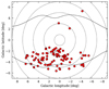 |
Fig. 1. Positions on the sky for the microlensed dwarf sample. The bulge contour lines based on observations with the COBE satellite are shown as solid lines (Weiland et al. 1994). The dotted lines are concentric circles in steps of 2°. The star that might not be located within the bulge boundaries (OGLE-2013-BLG0911S) is marked by a grey circle (see Bensby et al. 2017 for further discussion). |
3. Abundance analysis
3.1. Spectral lines and atomic data
To determine carbon abundances, we used six C I lines that are located in the near-infrared part of the spectrum in the 9060 to 9120 Å range. These C I lines are located in a region that is contaminated by telluric lines, meaning that before an abundance analysis can be performed, the telluric features must be removed from the bulge dwarf spectra. Therefore, for each target that was observed, we also observed a rapidly rotating B star during the same night, resulting in a featureless spectrum only containing the telluric lines (see Fig. 2). The red lines mark telluric lines with a line depth greater than about 15% of the continuum, and the orange lines mark those with a smaller depth. Also indicated by blue lines are the locations of the six C I lines. Depending on the radial velocity of the star, the carbon lines may, or may not, be blended by the telluric lines.
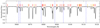 |
Fig. 2. Spectrum of a rapidly rotating B star containing only telluric absorption lines. The positions of the telluric lines are marked by red and orange lines (red lines deeper than orange ones, see Sect. 3.4), and the rest wavelengths of the six C I lines are marked with dotted blue lines. Depending on the (geocentric) radial velocity of the target, the C I lines will be either red- or blue-shifted and may, or may not, be contaminated by the telluric lines. |
Using the IRAF task TELLURIC, this spectrum can then be scaled and shifted slightly before it is used to divide out the telluric features in the observed spectrum of the bulge star. Figure 3 shows examples of the results of the telluric removal procedure for two of our targets. As can be seen, the procedure is efficient, generally leaving negligible traces of the telluric lines, allowing us to make use of even those C I lines that were directly aligned with the telluric absorption features.
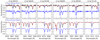 |
Fig. 3. C I lines in the 9060-9120 Å region. The top panel shows an example for MOA-2009-BLG-493S and the bottom panel an example for OGLE-2013-BLG-0446S. The black lines represent the observed spectrum, the red dash-dotted line represents a telluric template based on several observations of rapidly rotating B stars, and the blue lines represent the observed spectrum (vertically shifted for graphical reasons), after the removal of telluric features using the IRAF task TELLURIC. The vertical dashed lines mark the central wavelengths of the C I lines. We note that the spectra have been shifted to rest wavelengths and that the telluric lines will contaminate different lines depending on the radial velocity of the star. |
The two C I lines at 9063 Å and 9089 Å have asymmetric line profiles, and they are also shifted slightly off-centre relatively to the reference wavelengths. Figure 3 shows that this cannot be due to a poor removal of the telluric lines. The asymmetries and offsets of these two lines are caused by the presence of other blending spectral lines. In the case of the 9062 Å line there are several blending lines, but the main contributor is the Fe I line at 9062.2392 Å, and for the 9088 Å C I line there is an Fe I line at 9088.3177 Å. This makes the analysis of these C I lines challenging as the absorption profile usually is dominated by the blending line. However, we will keep them for the abundance analysis and then evaluate their usability (see Sect. 3.4).
We also considered the C I lines at 7111 and 7113 Å. But because these lines are weak they could rarely be discerned from the continuum noise, given the sometimes relatively low S/N, we decided not to use them.
The infrared O I triplet lines at 7772–7775 Å were used to determine oxygen abundances. In solar-type stars these lines are usually strong and clean as they are located in a wavelength region free from other blending lines and telluric lines (see example in Fig. 4). Another option would be to use the forbidden O I line at 6300 Å, but unfortunately that line is too weak to be used in the microlensed bulge dwarf spectra.
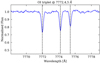 |
Fig. 4. O I triplet lines at 7772–7775 Å that have been investigated in this study. The blue lines represent the observed spectrum of OGLE-2013-BLG-0446S. The vertical dashed lines mark the central wavelengths of the three oxygen lines. |
Table 1 lists the atomic data for the C and O lines that were analysed. The atomic line data for the C I and O I lines, as well as the other spectral features in the region, were gathered from the Vienna Atomic Line Database (VALD, Piskunov et al. 1995; Ryabchikova et al. 1997, 2015; Kupka et al. 1999, 2000; Pakhomov et al. 2019).
Carbon and oxygen lines investigated in this study and the solar abundances that we determine from each line.
3.2. Line synthesis and NLTE corrections
The abundance analysis was done through a χ2-minimisation between the observed spectrum and a synthetic spectrum. The synthetic spectra were calculated with pySME, which is the python implementation of the spectroscopy made easy (SME) software (Valenti & Piskunov 1996; Piskunov & Valenti 2017).
To calculate a synthetic spectrum pySME needs atomic data (see above), stellar parameters, broadening parameters, and model stellar atmospheres. For the latter, we use the MARCS model atmospheres (Gustafsson et al. 2008), while Teff, log g, [Fe/H], and microturbulence are taken from our detailed analysis of the stars in Bensby et al. (2017).
In addition to atomic line broadening, the observed line profile is broadened by the instrument, the line-of-sight component of the stellar rotation (vrot ⋅ sin i), and small- and large-scale motions in the stellar atmosphere (microturbulence, ξt, and macroturbulence, vmacro, respectively). The instrument broadening is set by the resolving power of the spectrograph (R) and is treated with a Gaussian profile, while vrot ⋅ sin i and vmacro are jointly accounted for with a radial-tangential (RAD-TAN) profile. To determine the RAD-TAN broadening, other unblended, relatively weak, and unsaturated Fe I lines located at 6065, 6546, and 6678 Å were used. The C and O abundances for the different C I and O I lines were then determined through a simple χ2-minimisation routine that is illustrated in Fig. 5.
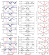 |
Fig. 5. Example showing the determination of carbon abundances from the six different C I lines (plots in the top six rows) and the three O I lines (plots in the bottom three rows). The plots in the left column show the observed spectrum as red lines and 20 synthetic spectra with carbon abundances in steps of 0.1 dex as black lines. The plots in the middle column show the differences between the observed and synthetic spectra. The plots in the right column shows the sum of the squared differences between observed and synthetic spectra within ±0.3 of the central wavelengths of the C I and O I lines (marked by black vertical dotted lines in the plots in the left column). The vertical red solid line shows the minimum of the χ2-values for which the best fitting carbon and oxygen abundances are selected. For each line, we carried out a local normalisation of the observed spectrum, and the selected continuum regions are marked by dotted red vertical lines in the plots in the left column. |
All of the C I and O I lines that are used in this study are sensitive to departures from the assumption of local thermodynamic equilibrium, and large NLTE corrections are needed to achieve reliable abundances (e.g., Asplund 2005; Amarsi et al. 2019b). For the oxygen triplet, in the previous papers (Bensby et al. 2009, 2011, 2013) we applied the empirical correction formula from Bensby et al. (2004), which studied the forbidden oxygen line at 6300 Å that is insensitive to departures from LTE (e.g., Asplund et al. 2004). However, that formula was based on a smaller sample of F and G dwarf stars that do not cover the full range of stellar parameters that are spanned by the microlensed dwarf sample. Instead, we now make use of the tables of NLTE departure coefficients, for both C and O, from Amarsi et al. (2020), which are implemented directly into pySME.
Abundances of iron, carbon, and oxygen for all stars and all lines are given in Table 2. Also included in Table 2 are flags that indicate whether the individual C I lines are close to a weak or a strong telluric line or not at all.
Carbon and oxygen abundances (NLTE) and their associated uncertainties.
3.3. Solar analysis
The derived abundances have been normalised to the Sun on a line-by-line basis. The solar analysis was carried out on spectra obtained through observations of the asteroids Vesta and Ceres. This means that rather than taking a standard value for the Sun, we determine our own oxygen and carbon abundances for each and every line that we analyse and use those to normalise the individual line abundances. In that way, we minimise systematic uncertainties that are likely to arise because of the analysis methods and atomic data that are used. Our analysis is therefore truly differential to the Sun. Table 1 gives our carbon and oxygen results for the Sun. As can be seen, they are internally consistent and compare well with the abundances derived by, for instance, Amarsi et al. (2019a), who performed a 3D NLTE line formation analysis of neutral carbon in the Sun (A(C) = 8.44), and Amarsi et al. (2018), who found A(O) = 8.69 from the O I triplet lines, again using 3D NLTE models. The NLTE corrected solar abundances listed in Table 1 have been used to normalise the abundances on a line-by-line basis.
3.4. Abundances from individual lines
Figure 6 shows the [C/Fe]–[Fe/H] trends based on carbon abundances from the individual C I lines. Here, we mark the stars where the line centre of the C I line that the carbon abundance is based on falls within ±0.3 Å of a telluric line (orange marker if it is one of the weaker telluric lines and a red marker if it is one of the stronger telluric lines, as shown in Fig. 2). In each plot, we also indicate the median [C/Fe] value and the dispersion in [C/Fe]. First we note that all six C I lines are able to give carbon abundances that result in very similar [C/Fe] − [Fe/H] abundance trends, even the two lines at 9063 Å and 9089 Å that were blended by other Fe I lines in the stellar spectrum. We also note that there are no particular trends for those stars whose lines originally were originally located close to the telluric lines. This is further illustrated in Fig. 7, which shows the [C/Fe] − [Fe/H] trends based on the average abundance from all six C I lines, with the top plot including all lines, the middle plot including those lines that were unaffected by telluric lines or close to one of the weaker telluric lines (orange lines in Fig. 2), and the bottom plot only showing the lines that were completely unaffected by telluric lines. The median [C/Fe] values and the dispersions in [C/Fe] are very similar in all three cases (the numbers are given in Fig. 2). The three plots are very similar, confirming that the removal of the telluric lines from the microlensed dwarf star spectra has been successful.
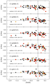 |
Fig. 6. [C/Fe]–[Fe/H] trend based on individual C I lines (as indicated in the plots). Black circles indicate that the C I line in question have not been affected by a telluric line, orange circles mean that the line in question has been located closer than 0.3 Å to a telluric line with a depth weaker than 15% of the continuum, and the red circles mean that the line in question is located closer than 0.3 Å to one of the stronger telluric lines. The telluric lines are marked in Fig. 2. In each plot, we also indicate the median [C/Fe] value and the dispersion in [C/Fe]. |
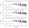 |
Fig. 7. [C/Fe]–[Fe/H] trends where the carbon abundances are based on the mean abundance coming from the different C I lines. In the top plot, all C I lines are included in the calculation of the mean C abundance for each star; in the middle plot C I lines located close to strong telluric lines (red marked lines in Fig. 2) were excluded when calculating the mean C abundance for each star; and in the bottom plot, all C I lines located close to a telluric line (orange and red lines in Fig. 2 and orange and red points in Fig. 6) were excluded from the calculation of the mean C abundance for each star. In each plot, we also indicate the median [C/Fe] value and the dispersion in [C/Fe]. |
As there is no clear indication that any of the six C I lines produce unusual C abundances, the discussion and figures are henceforth based on the average C abundances inferred from all six lines (whenever available).
3.5. Error analysis
Random uncertainties in the derived carbon and oxygen abundances are estimated by taking the uncertainties in the stellar parameters (Teff, log g, [Fe/H], and ξt) into consideration. The changes in the abundances that are acquired by changing the stellar parameters are then added in quadrature (this is a relatively easy, and commonly used, way to estimate uncertainties, but it assumes that the uncertainties in the stellar parameters are un-correlated, which might not be completely true). The uncertainties are given in Table 2 and also shown in Fig. 8.
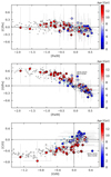 |
Fig. 8. [C/Fe] versus [Fe/H] (top panel), [O/Fe] versus [Fe/H] (middle panel), and [C/O] versus [O/H] (bottom panel) for the microlensed bulge dwarf sample. The bulge stars are colour-coded based on their ages, according to the colour bar on the right hand side. Light red circles and light blue dots are solar-neighbourhood thick- and thin-disk dwarf stars, respectively (oxygen based on the forbidden [O I] line at 6300 Å from Bensby et al. 2004, 2005 and carbon based on the forbidden [C I] line at 8727 Å from Bensby & Feltzing 2006). Large grey circles in the [C/H]–[O/H] plot are halo stars from Akerman et al. (2004), and small grey dots (in all plots) are the disk and halo stars (1D, NLTE results) from Amarsi et al. (2019b). In the oxygen plots, the positions of MOA-2010-BLG-523S are marked. In the carbon plot at the top, MOA-2010-BLG-523S has a [C/Fe] value very close to solar. |
Systematic uncertainties should be minimised as we are doing a strictly differential analysis to the Sun. The stars have quite similar parameters relative to each other and relative to the Sun so differential systematic errors due to, for example, 3D, non-LTE, stellar parameters, and line broadening should be small (and uncertainties due to atomic data errors largely cancel). By confirming that the different spectral lines give consistent abundances and very similar abundance trends (see Fig. 6), we also are confident that there should be no major systematic offsets.
4. Results
Figure 8 shows the [C/Fe] − [Fe/H], [O/Fe] − [Fe/H], and [C/O] − [O/H] abundance trends for the microlensed bulge dwarf sample. For comparison purposes, the plots also include stars representing the Galactic thin and thick disks where the abundances are based on the forbidden C I and O I lines at 8727 Å and 6300 Å, respectively (Bensby et al. 2004, 2005; Bensby & Feltzing 2006). These forbidden lines are not sensitive to departures from the assumption of LTE (e.g., Asplund et al. 2004, 2005). The sample from Amarsi et al. 2019b that presented an analysis of C and O for 187 nearby disk and halo stars is also included (the 1D, NLTE results from Amarsi et al. 2019b are shown here). In the [C/O] − [O/H] plot, we further include the halo sample from Akerman et al. (2004), based on NLTE-corrected abundances from the same C and O lines analysed in this study. These disk and halo trends compare well with the Amarsi et al. (2019b) results.
For the microlensed dwarf stars, as well as the comparison samples, the [C/Fe] ratios tend to be slightly enhanced compared to the Sun for metallicities up to [Fe/H] ≈ 0, and thereafter they decline towards higher [Fe/H]. A slight difference in the details is that Amarsi et al. (2019b) see a separation in the [C/Fe]–[Fe/H] diagram between thin- and thick-disk stars, while Bensby & Feltzing (2006) do not see that. An explanation could be that the two studies use different ways of defining thin- and thick-disk stars: Amarsi et al. (2019b) used chemical criteria (as defined by Adibekyan et al. 2013), while Bensby & Feltzing (2006) used kinematical criteria. In this study, we used age criteria, as advocated for in Bensby et al. (2014), where thin-disk stars are likely to be younger than 8 Gyr, and thick-disk stars are likely to be older than 8 Gyr. It should be noted that the overall appearance of the [C/Fe] − [Fe/H] trend in the disk is very similar between the two studies. This also holds for the [O/Fe] − [Fe/H] trend, where Bensby et al. (2004, 2005) agree well with Amarsi et al. (2019b); that is, a clear distinction between the thin and thick disks at sub-solar [Fe/H] and a continued, rather steep decline in [O/Fe] towards higher [Fe/H].
4.1. Carbon in the bulge
The evolution of [C/Fe] varies essentially in lockstep with [Fe/H] for the microlensed bulge dwarf stars. There is a slight tendency of a carbon over-abundance at sub-solar metallicities and a carbon under-abundance at super-solar metallicities, that also can be interpreted as a shallow decline in [C/Fe] with [Fe/H]. The [C/Fe] trend for the stars younger than about 8 Gyr follow smoothly upon the trend for the stars older than about 8 Gyr, and there is no indication of a separation in [C/Fe] between the stars in the two age groups. Comparisons to the local thin- and thick-disk samples from Bensby & Feltzing (2006) to the < 8 Gyr and > 8 Gyr sub-samples show that the microlensed bulge dwarf [C/Fe] trends are very similar to what is observed in the nearby Galactic thin and thick disks.
4.2. Oxygen in the bulge
The [O/Fe] − [Fe/H] trend for the microlensed dwarf stars shows the typical signature abundance trend seen for the other α-elements (Bensby et al. 2017); that is, an enhanced [O/Fe] ratio that declines towards solar metallicities for the stars older than about 8 Gyr and a more shallow separated decline for the stars younger than about 8 Gyr. At super-solar metallicities, the [O/Fe] − [Fe/H] trend continues to decrease, in contrast to the other α-elements, but in agreement with the [O/Fe] trend in the local disk (as also seen in, for example, Alves-Brito et al. 2010, but for a much smaller sample).
The agreement between the bulge and local disk trends are striking, but with a reservation that the bulge [O/Fe] abundance ratios might be slightly more enhanced than what is seen in the local thick disk. Although it could not be statistically verified, in Bensby et al. (2017) we suggested that this apparent enhancement could be because the position of the ‘knee’ in the bulge is located at a metallicity that is about 0.1 dex higher than in the thick disk. On the other hand, Griffith et al. (2021) conclude that the differences between the bulge and local disk stars seen in several studies are due to sampling effects with bulge samples generally containing more evolved stars, and if this bias is compensated for, the differences vanish. Moreover, Zasowski et al. (2019) found that the position of the knee in the α-element abundance trends is constant with galactocentric radius in the Galactic disk.
4.3. Carbon-over-oxygen in the bulge
The bottom plot in Fig. 8 shows the [C/O] − [O/H] abundance plane for the microlensed bulge dwarf stars, and it shows how the old and young stars in the bulge divide into the two distinct and well-separated sequences as outlined by the solar neighbourhood thin and thick disks. The metal-poor end of the sample aligns with the [C/O] ratios observed in the stellar halo samples by Akerman et al. (2004) and Amarsi et al. (2019b).
4.4. Outliers
Even though the overall carbon and oxygen abundance trends shown in Fig. 8 are well-defined and tend to follow what is observed locally in the Galactic disk, there are a few stars that deviate. In particular, there is one star in the [C/O] − [O/H] plot (MOA-2010-BLG-523S with [C/O] = −0.39 at [O/H] = 0.44) and perhaps three stars (marked as younger than 8 Gyr) with high [O/Fe] values around solar metallicities in the [O/Fe] − [Fe/H] plot. We checked the analysis of those stars extremely carefully; in particular, we wanted to ascertain whether their spectra have unusually low S/N, whether the fitting of the synthetic spectra are bad, and whether they have stellar parameter uncertainties that are unusually high, but no such indications were seen.
Regarding MOA-2010-BLG-523S (with [C/O] = −0.39 at [O/H] = 0.44, and [O/Fe] = +0.38 and [C/Fe] = −0.01 at [Fe/H] = 0.06), we note that this star actually was deemed by Gould et al. (2013) to be an RS CVn star in the bulge. If this is so, it might be that the measured abundance ratios are affected, and in particular the NLTE effects of the abundances from the O I triplet lines are very large, which could lead to severely overestimated photospheric oxygen abundances of up to 0.5–1.5 dex (Morel et al. 2006). Thus this could explain the very high [O/H] ratio leading to the very low [C/O] ratio. In the [O/Fe] − [Fe/H] and [C/O] − [O/H] plots in Fig. 8, MOA-2010-BLG-523S is marked out but not in the [C/Fe] − [Fe/H] plot as its [C/Fe] value does not stand out compared to the other stars.
If MOA-2010-BLG-523S is indeed an RS CVn star, and depending on how high its activity index is, its stellar parameters might also have been affected. According to Spina et al. (2020), it is mainly the microturbulence parameter that is affected, and overestimated, which would lead to too low [Fe/H] values of up to 0.1 dex. The surface gravity appears essentially unaffected, while the effective temperature could be underestimated by up to a few hundred degrees for stars that have high activity indices. We do not know the actual activity index of MOA-2010-BLG-523S, but as was pointed out in Gould et al. (2013) its microturbulence deviates from the other stars in the sample, which in turn could mean that its temperature also could be underestimated. Figure 9 shows MOA-2010-BLG-523S in an HR diagram with matching isochrones over-plotted. A higher metallicity of up to 0.1 dex and a higher temperature of up to a few hundred degrees would probably not change the estimated age of MOA-2010-BLG-523S by much as it will only move horizontally to the left in the HR diagram. Hence, it is clear that this is still a young star located in the Galactic bulge.
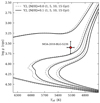 |
Fig. 9. Position of MOA-2010-BLG-523S in the HR diagram. Two sets of isochrones from Demarque et al. (2004) are plotted with metallicities as indicated in the figure. For each set of isochrones the ages of 1, 5, 10, and 15 Gyr are shown. If the star is indeed an RS CVn star, its metallicity is probably too low by up to 0.1 dex, and its effective temperature is too low by a few hundred degrees, while its surface gravity is likely to be unchanged. As can be seen, that change has essentially no effect on its estimated age. |
5. Discussion
5.1. Comparisons to chemical evolution models
In the following discussion, we make comparisons of the observed abundance trends to the models of Galactic chemical evolution (GCE) presented by Romano et al. (2020) that include yields from low- and intermediate-mass stars from Ventura et al. (2013) and yields from rotating high-mass stars from Limongi & Chieffi (2018). The first model is the MWG-11 model of the solar vicinity from Romano et al. (2019), which is based on the two-infall models originally developed by Chiappini et al. (1997) but revised (MWG-11 rev) according to the prescriptions of Spitoni et al. (2019). This model includes the stellar nucleosynthetic yields by rotating massive stars that vary with metallicity; at low metallicities below [Fe/H] < − 1, the maximum rotational velocity of 300 km s−1 was applied but reduced to 0 km s−1 at solar metallicities. The second model is the parallel thin- and thick-disk model by Grisoni et al. (2017), in which the two disks evolve independently, but with updated stellar nucleosynthetic yields from massive stars rotating at different rotational velocities (0, 150, or 300 km s−1). The last model that we adopt from Romano et al. (2020) is the bulge model by Matteucci et al. (2019) that assumes that all stars are old and formed in an early starburst; that is, a so-called classical bulge formation scenario (also here with the nucleosynthetic yields of rotating massive stars at different velocities of 0, 150, or 300 km s−1). By default, the GCE models by Romano et al. (2020) were normalised to the Lodders et al. (2009) solar abundance scale, but here they are re-normalised to the Asplund et al. (2021) solar abundance scale.
The different models are shown in Fig. 10 together with the new abundance results for the microlensed bulge dwarf stars. The upper panel shows the C and O trends with Fe as a reference element, and the lower panel shows the C trends with O as a reference element.
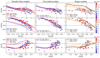 |
Fig. 10. Comparisons of the observed carbon and oxygen abundance trends to the different GCE models from Romano et al. (2020). Left hand side plots: Parallel model for thin disk (blue lines) and thick disk (red lines) by Grisoni et al. (2017) with updated stellar nucleosynthetic yields from Romano et al. (2019), here for massive stars rotating at either zero (dotted lines) or 300 km s−1 (solid lines). Middle plots: Two-infall MWG-11 model from Romano et al. (2019) but revised according to the prescriptions in Spitoni et al. (2019) (dark purple dashed lines) and without the revision by Spitoni et al. (2019) (solid purple lines). Right hand side plots: Bulge models by Matteucci et al. (2019) with the nucleosynthetic yields of the MWG-05, MWG-06, and MWG-07 models by Romano et al. (2019), which includes rapidly rotating massive stars at 300, 150, and 0 km s−1, respectively. |
Lastly, before going into the comparison of the GCE models to the observational data, we caution that GCE models, as stated by Romano et al. (2020), by construction predict the climate but not the weather, and they are only meant to reproduce the average trends and cannot account for the spread in the observed data2.
5.1.1. Parallel thin- and thick-disk models
The parallel thin- and thick-disk models with two sets of yields from rotating massive stars, 0 km s−1 and 300 km s−1, respectively, are shown in the plots on the left hand side in Fig. 10. The observed [C/Fe] − [Fe/H] data are relatively well-matched by the model version where the massive stars are non-rotating, while the [O/Fe] − [Fe/H] trend is well-matched by the model version in which the massive stars are rotating at 300 km s−1. The combined evolution of C and O in the [C/O] − [O/H] plane shows that the best matching models are the ones with yields from massive stars rotating at 300 km s−1. This good match is driven by the good match of oxygen to models with yields from rapidly rotating massive stars, and it is difficult to evaluate whether this is also a good match for carbon (this is unlikely). A solution might be that the C yields from rapidly rotating massive stars should be lowered (as the match of oxygen is so good in the [O/Fe] − [Fe/H] plane, and as oxygen is generally believed to have a well-understood nucleosynthetic origin). If that were the case, the parallel thin- and thick-disk GCE models would be able to better match the observed data in the [C/Fe] − [Fe/H] and [C/O] − [O/H] planes. It should be noted that Limongi & Chieffi (2018) use the 12C(α, γ)16O rate from Kunz et al. (2002), which could result in an overproduction of carbon.
5.1.2. Two-infall models
The two-infall models shown in the middle column of Fig. 10 are able to match the observations reasonably well. The best agreement is seen for oxygen in the [O/Fe] − [Fe/H] plane, while they appear to produce slightly too much carbon in the [C/Fe] − [Fe/H] plane (as was also seen for the parallel thin- and thick-disk models). If the C yields from massive stars could have been reduced, an overall better match in both the [C/Fe] − [Fe/H] and [C/O] − [O/H] could have been reached. It is worth stressing that the models discussed up to now are calibrated on the solar vicinity. In the next section, we compare the data to models specifically tailored to the Galactic bulge.
5.1.3. Bulge models
The bulge models shown in the plots in the right hand side column in Fig. 10 are not in agreement with the observations. The models with yields from rapidly rotating massive stars do not match either of the [C/Fe] − [Fe/H] or [O/Fe] − [Fe/H] trends. In both cases, the C and O abundances are too elevated in the models. The models with yields from non-rotating massive stars are partly able to follow some parts of the observations, but the overall match is rather poor. The situation improves when considering the [C/O] − [O/H] plane, but that improvement is clearly due to the fact that the poor matches on the two other planes are cancelled out to some degree. It is clear that the overall appearance of the GCE models is not similar to the observed abundance data in the bulge.
5.2. The origin of carbon in the bulge
The overall good agreement between the two-infall and the parallel disk models to the observed abundance trends in the bulge is a striking feature as what we are comparing is bulge abundance trends to GCE models made to simulate the Galactic disk in the solar vicinity. Grisoni et al. (2018) expanded these models to other galactocentric radii, and even though the star formation rate is much higher at distances closer to the centre of the Galaxy, the overall appearance of the abundance trends does not seem to vary much for the two-infall model.
In the early times of the Milky Way, it is clear that the enrichment of the interstellar medium must come from massive stars, as it is those that can contribute on short timescales. The good match of the oxygen trends to the models (both parallel and two-infall) with yields from rapidly rotating massive stars is reassuring as oxygen is the element that we believe has a very clean and well-understood origin (e.g., Woosley & Weaver 1995). The slight mismatch of the carbon trends would then mean that the prescriptions that went into the yield calculations of massive stars result in too much carbon being produced. From the [C/O] − [O/H] abundance trends, we further see that it is when the low- and intermediate mass stars start to contribute to the enrichment that the [C/O] ratio rapidly increases. Alternatively, metallicity-dependent C yields from massive stars can result in higher C production at high metallicities (Maeder 1992; Prantzos et al. 1994).
Romano et al. (2020) conclude that at least 60 % of the carbon in the disk comes from massive stars, and the fraction is even higher for stars in the bulge. The agreement between the elemental abundance trends in the bulge and the thin and thick disks in the solar neighbourhood tells us that not only are the bulge and the disk(s) intimately connected, if not the same, but also that the origin of carbon is the same in both regions.
It is clear that the solution is not easy, and both observational and theoretical studies come to differing solutions regarding the importance of, and relative contributions of, carbon production from low-, intermediate-, and high-mass stars (e.g., Cescutti et al. 2009; Mattsson 2010; Franchini et al. 2020, and references therein). Our observations seem to favour the notion that the fraction of carbon being made in massive stars is lower, although how much lower we cannot say: more detailed GCE models and stellar yield calculations are needed to explore that question.
5.3. Traces of a classical bulge
The formation of the bulge has long been regarded as having occurred on very short timescales (e.g., Matteucci & Brocato 1990; Ballero et al. 2007; Cescutti & Matteucci 2011; Renzini et al. 2018). However, recent observational data suggest that most of the stars in the bulge region could have a secular origin made from disk material (e.g., Meléndez et al. 2008; Shen et al. 2010), which is also supported by the results from the microlensed dwarf stars (Bensby et al. 2017) with their wide range of ages, complex metallicity distribution with two or more peaks (see also, e.g., Hill et al. 2011; Ness et al. 2013; Zoccali et al. 2017; Rojas-Arriagada et al. 2017, 2020), and detailed elemental abundance trends that mimic the ones of the local thin and thick disks (see also, e.g., Alves-Brito et al. 2010; Johnson et al. 2014; Gonzalez et al. 2015; Jönsson et al. 2017). However, that does not mean that we can rule out that some of the stars in the bulge region do originate from an early intense star formation event that can be associated with a classical bulge scenario. The question is, how large could that part be?
In the C and O abundance plots in Figs. 8 and 10, there are some stars that appear to deviate from the general abundance trends, maybe even forming a separate trend of their own. In Fig. 11, we plot the abundance trends again but highlight these stars, as well as some stars at lower [O/H] values that align with these deviating stars at higher [O/H], with yellow circles. In the [O/Fe] − [Fe/H] plane, these stars tend to be located at slightly more enhanced levels, much in the same way that the bulge in general has purportedly shown slightly more elevated α-element abundances than the local thick disk (Bensby et al. 2013; Johnson et al. 2014; Bensby et al. 2017; Jönsson et al. 2017). Could it be that these slightly elevated stars actually belong to another sub-group of stars in the bulge region? In the [C/Fe] − [Fe/H] plane, these deviating stars are, on average, less carbon-enhanced than the other stars at similar metallicities. They are more or less perfectly in lock-step with [Fe/H], and perhaps just below solar-metallicity they tend to be under-abundant. The selected yellow stars in Fig. 11 does not show much agreement with either of the GCE models in Fig. 10. A match between the GCE bulge models shown in the plots on the right hand side of Fig. 10, and the observations would be possible if the C yields from massive stars are decreased significantly.
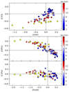 |
Fig. 11. [C/O] − [O/H] trend where the low-[C/O] stars are defined and marked by yellow circles. These are then also marked in the [O/Fe], and [C/Fe] versus [Fe/H] plots. |
If the 11 chemically distinct yellow points in Fig. 11 are drawn from a population with a distinct origin, such as a ‘classical bulge’, then this might be reflected in distinct kinematics as well. However, a comparison of the galactocentric radial velocities of these stars to the other stars in the sample with ages greater than eight billion years showed no significant differences. Additionally, other parameters such as the age distribution and the distributions in galactic longitude and latitude do not reveal any deviating properties for these stars. Therefore, in conclusion, even though it is tempting to associate these stars with a classical bulge population, more work and possibly also a larger sample of stars is needed to definitively confirm such connections.
6. Summary
We present a detailed analysis of carbon and oxygen for a sample of 91 microlensed dwarf and subgiant stars in the Galactic bulge. Carbon abundances for 70 stars were determined from line synthesis of six C I in the wavelength range 9060–9120 Å, and oxygen abundances for 88 stars from line synthesis of the three O I lines at 7772–7775 Å. NLTE corrections were accounted for when calculating the synthetic spectra. As the stars have not reached the evolved giant star phase, the estimated C and O surface abundances have not been affected by internal nucleosynthetic burning processes and therefore reflect the carbon and oxygen abundances of the gas clouds that the stars were born from. Our main findings are summarised as follows:
-
The abundance trends that contain oxygen in the Galactic bulge have the same appearance as seen for other α-elements. The one distinction is that at super-solar abundances, oxygen continues to decline, whereas other α-elements such as Mg, Ca, and Ti, level out and vary in lockstep with Fe towards the highest metallicities. The most accepted explanation is that oxygen has metallicity-dependent yields.
-
Carbon in the Galactic bulge has a similar appearance as seen for Fe; that is, it is mainly scattering around solar [C/Fe] at all [Fe/H]. When comparing carbon to oxygen, the [C/O]–[O/H] trend is very similar to what is seen for [Fe/H]–[O/H].
-
Both carbon and oxygen trends in the Galactic bulge are very similar to what is observed locally in the solar neighbourhood in the Galactic thin and thick disks. The old part (older than eight billion years) follows the thick disk, while the young part (younger than eight billion years) follows the thin disk.
-
Galactic chemical evolution models for the thin and thick disks agree well with the observed [C/O]–[O/H] trends in the bulge. Specially tailored chemical evolution models for the bulge, in which the bulge is represented by a single spheroid, do not match the observed data as well. Hence, the observations point to a secular origin of the Galactic bulge, in which the majority of the stellar population in the inner parts of the Galaxy is formed from existing disk populations. We note that this does not rule out the existence of a small classical bulge component. However, we cannot say how large it is.
Our findings do not support the recent suggestions that carbon should, to a higher degree, originate from massive stars in the bulge than elsewhere in the disk. Contrarily, our results, that the carbon trends in the bulge and the thin and thick disks agree well, shows that the fraction of carbon being made by massive stars in the bulge should be lower and similar to what is observed in the Galactic disk(s).
IRAF is distributed by the National Optical Astronomy Observatories, which are operated by the Association of Universities for Research in Astronomy, Inc., under a cooperative agreement with the National Science Foundation (Tody et al. 1986, 1993).
There is speculation that the this wise saying comes from Steve Shore: “They [GCE models] are a way to study the climate, not the weather, in galaxies” (as reported by Monica Tosi in some conference proceedings...; Donatella Romano, priv. comm.).
Acknowledgments
T.B. was funded by grant No. 2018-04857 from The Swedish Research Council. J.M. thanks FAPESP (2014/18100-4). We are grateful to Donatella Romano for providing their Galactic chemical evolution models in machine readable format and for providing valuable comments on a draft version of the paper. We also thank the anonymous referee for valuable comments that improved the clarity of the paper. This work has made use of the VALD database, operated at Uppsala University, the Institute of Astronomy RAS in Moscow, and the University of Vienna. This research made use of Astropy, a community-developed core Python package for Astronomy (Astropy Collaboration 2013), Matplotlib (Hunter 2007), and NumPy (Harris et al. 2020).
References
- Adibekyan, V. Z., Figueira, P., Santos, N. C., et al. 2013, A&A, 554, A44 [NASA ADS] [CrossRef] [EDP Sciences] [Google Scholar]
- Akerman, C. J., Carigi, L., Nissen, P. E., Pettini, M., & Asplund, M. 2004, A&A, 414, 931 [NASA ADS] [CrossRef] [EDP Sciences] [Google Scholar]
- Alves-Brito, A., Meléndez, J., Asplund, M., Ramírez, I., & Yong, D. 2010, A&A, 513, A35 [NASA ADS] [CrossRef] [EDP Sciences] [Google Scholar]
- Amarsi, A. M., Barklem, P. S., Asplund, M., Collet, R., & Zatsarinny, O. 2018, A&A, 616, A89 [NASA ADS] [CrossRef] [EDP Sciences] [Google Scholar]
- Amarsi, A. M., Nissen, P. E., & Skúladóttir, Á. 2019a, A&A, 630, A104 [NASA ADS] [CrossRef] [EDP Sciences] [Google Scholar]
- Amarsi, A. M., Barklem, P. S., Collet, R., Grevesse, N., & Asplund, M. 2019b, A&A, 624, A111 [NASA ADS] [CrossRef] [EDP Sciences] [Google Scholar]
- Amarsi, A. M., Lind, K., Osorio, Y., et al. 2020, A&A, 642, A62 [EDP Sciences] [Google Scholar]
- Asplund, M. 2005, ARA&A, 43, 481 [Google Scholar]
- Asplund, M., Gustafsson, B., Kiselman, D., & Eriksson, K. 1997, A&A, 318, 521 [NASA ADS] [Google Scholar]
- Asplund, M., Grevesse, N., Sauval, A. J., Allende Prieto, C., & Kiselman, D. 2004, A&A, 417, 751 [NASA ADS] [CrossRef] [EDP Sciences] [Google Scholar]
- Asplund, M., Grevesse, N., Sauval, A. J., Allende Prieto, C., & Blomme, R. 2005, A&A, 431, 693 [NASA ADS] [CrossRef] [EDP Sciences] [Google Scholar]
- Asplund, M., Amarsi, A. M., & Grevesse, N. 2021, A&A, 653, A141 [NASA ADS] [CrossRef] [EDP Sciences] [Google Scholar]
- Astropy Collaboration (Robitaille, T. P., et al.) 2013, A&A, 558, A33 [NASA ADS] [CrossRef] [EDP Sciences] [Google Scholar]
- Ballero, S. K., Matteucci, F., Origlia, L., & Rich, R. M. 2007, A&A, 467, 123 [NASA ADS] [CrossRef] [EDP Sciences] [Google Scholar]
- Bensby, T., & Feltzing, S. 2006, MNRAS, 367, 1181 [CrossRef] [Google Scholar]
- Bensby, T., Feltzing, S., & Lundström, I. 2004, A&A, 415, 155 [NASA ADS] [CrossRef] [EDP Sciences] [Google Scholar]
- Bensby, T., Feltzing, S., Lundström, I., & Ilyin, I. 2005, A&A, 433, 185 [NASA ADS] [CrossRef] [EDP Sciences] [Google Scholar]
- Bensby, T., Johnson, J. A., Cohen, J., et al. 2009, A&A, 499, 737 [NASA ADS] [CrossRef] [EDP Sciences] [Google Scholar]
- Bensby, T., Feltzing, S., Johnson, J. A., et al. 2010, A&A, 512, A41 [NASA ADS] [CrossRef] [EDP Sciences] [Google Scholar]
- Bensby, T., Adén, D., Meléndez, J., et al. 2011, A&A, 533, A134 [NASA ADS] [CrossRef] [EDP Sciences] [Google Scholar]
- Bensby, T., Yee, J. C., Feltzing, S., et al. 2013, A&A, 549, A147 [NASA ADS] [CrossRef] [EDP Sciences] [Google Scholar]
- Bensby, T., Feltzing, S., & Oey, M. S. 2014, A&A, 562, A71 [NASA ADS] [CrossRef] [EDP Sciences] [Google Scholar]
- Bensby, T., Feltzing, S., Gould, A., et al. 2017, A&A, 605, A89 [NASA ADS] [CrossRef] [EDP Sciences] [Google Scholar]
- Bensby, T., Feltzing, S., Yee, J. C., et al. 2020, A&A, 634, A130 [NASA ADS] [CrossRef] [EDP Sciences] [Google Scholar]
- Bertran de Lis, S., Allende Prieto, C., Majewski, S. R., et al. 2016, A&A, 590, A74 [NASA ADS] [CrossRef] [EDP Sciences] [Google Scholar]
- Biemont, E., & Zeippen, C. J. 1992, A&A, 265, 850 [NASA ADS] [Google Scholar]
- Cescutti, G., & Matteucci, F. 2011, A&A, 525, A126 [NASA ADS] [CrossRef] [EDP Sciences] [Google Scholar]
- Cescutti, G., Matteucci, F., McWilliam, A., & Chiappini, C. 2009, A&A, 505, 605 [NASA ADS] [CrossRef] [EDP Sciences] [Google Scholar]
- Charbonnel, C. 1994, A&A, 282, 811 [NASA ADS] [Google Scholar]
- Chiappini, C., Matteucci, F., & Gratton, R. 1997, ApJ, 477, 765 [Google Scholar]
- Chiappini, C., Romano, D., & Matteucci, F. 2003, MNRAS, 339, 63 [NASA ADS] [CrossRef] [Google Scholar]
- Cohen, J. G., Thompson, I. B., Sumi, T., et al. 2009, ApJ, 699, 66 [NASA ADS] [CrossRef] [Google Scholar]
- Demarque, P., Woo, J.-H., Kim, Y.-C., & Yi, S. K. 2004, ApJS, 155, 667 [NASA ADS] [CrossRef] [Google Scholar]
- Edvardsson, B., Andersen, J., Gustafsson, B., et al. 1993, A&A, 275, 101 [NASA ADS] [Google Scholar]
- Franchini, M., Morossi, C., Di Marcantonio, P., et al. 2020, ApJ, 888, 55 [NASA ADS] [CrossRef] [Google Scholar]
- Gonzalez, O. A., Zoccali, M., Vasquez, S., et al. 2015, A&A, 584, A46 [NASA ADS] [CrossRef] [EDP Sciences] [Google Scholar]
- Gould, A., Yee, J. C., Bond, I. A., et al. 2013, ApJ, 763, 141 [NASA ADS] [CrossRef] [Google Scholar]
- Griffith, E., Weinberg, D. H., Johnson, J. A., et al. 2021, ApJ, 909, 77 [NASA ADS] [CrossRef] [Google Scholar]
- Grisoni, V., Spitoni, E., Matteucci, F., et al. 2017, MNRAS, 472, 3637 [Google Scholar]
- Grisoni, V., Spitoni, E., & Matteucci, F. 2018, MNRAS, 481, 2570 [NASA ADS] [Google Scholar]
- Gustafsson, B., Bell, R. A., Eriksson, K., & Nordlund, A. 1975, A&A, 42, 407 [NASA ADS] [Google Scholar]
- Gustafsson, B., Karlsson, T., Olsson, E., Edvardsson, B., & Ryde, N. 1999, A&A, 342, 426 [NASA ADS] [Google Scholar]
- Gustafsson, B., Edvardsson, B., Eriksson, K., et al. 2008, A&A, 486, 951 [NASA ADS] [CrossRef] [EDP Sciences] [Google Scholar]
- Haris, K., & Kramida, A. 2017, ApJS, 233, 16 [Google Scholar]
- Harris, C. R., Millman, K. J., van der Walt, S. J., et al. 2020, Nature, 585, 357 [NASA ADS] [CrossRef] [Google Scholar]
- Hibbert, A., Biemont, E., Godefroid, M., & Vaeck, N. 1991, J. Phys. B At. Mol. Phys., 24, 3943 [NASA ADS] [CrossRef] [Google Scholar]
- Hibbert, A., Biemont, E., Godefroid, M., & Vaeck, N. 1993, A&AS, 99, 179 [Google Scholar]
- Hill, V., Lecureur, A., Gómez, A., et al. 2011, A&A, 534, A80 [NASA ADS] [CrossRef] [EDP Sciences] [Google Scholar]
- Hunter, J. D. 2007, Comput. Sci. Eng., 9, 90 [NASA ADS] [CrossRef] [Google Scholar]
- Johnson, J. A., Gaudi, B. S., Sumi, T., Bond, I. A., & Gould, A. 2008, ApJ, 685, 508 [NASA ADS] [CrossRef] [Google Scholar]
- Johnson, C. I., Rich, R. M., Kobayashi, C., Kunder, A., & Koch, A. 2014, AJ, 148, 67 [Google Scholar]
- Jönsson, H., Ryde, N., Schultheis, M., & Zoccali, M. 2017, A&A, 598, A101 [NASA ADS] [CrossRef] [EDP Sciences] [Google Scholar]
- Jørgensen, B. R., & Lindegren, L. 2005, A&A, 436, 127 [Google Scholar]
- Kormendy, J., & Kennicutt, R. C. 2004, ARA&A, 42, 603 [Google Scholar]
- Kunz, R., Fey, M., Jaeger, M., et al. 2002, ApJ, 567, 643 [CrossRef] [Google Scholar]
- Kupka, F., Piskunov, N., Ryabchikova, T. A., Stempels, H. C., & Weiss, W. W. 1999, A&AS, 138, 119 [NASA ADS] [CrossRef] [EDP Sciences] [Google Scholar]
- Kupka, F. G., Ryabchikova, T. A., Piskunov, N. E., Stempels, H. C., & Weiss, W. W. 2000, Balt. Astron., 9, 590 [Google Scholar]
- Lagarde, N., Reylé, C., Robin, A. C., et al. 2019, A&A, 621, A24 [NASA ADS] [CrossRef] [EDP Sciences] [Google Scholar]
- Limongi, M., & Chieffi, A. 2018, ApJS, 237, 13 [NASA ADS] [CrossRef] [Google Scholar]
- Lind, K., Bergemann, M., & Asplund, M. 2012, MNRAS, 427, 50 [Google Scholar]
- Lodders, K., Palme, H., & Gail, H. P. 2009, 4.4 Abundances of the elements in the Solar System: Datasheet from Landolt-Börnstein - Group VI Astronomy and Astrophysics. Volume 4B: "Solar System" in SpringerMaterials (Berlin Heidelberg: Springer-Verlag), https://dx.doi.org/10.1007/978-3-540-88055-4_34 [Google Scholar]
- Maeder, A. 1992, A&A, 264, 105 [NASA ADS] [Google Scholar]
- Matteucci, F., & Brocato, E. 1990, ApJ, 365, 539 [CrossRef] [Google Scholar]
- Matteucci, F., Grisoni, V., Spitoni, E., et al. 2019, MNRAS, 487, 5363 [Google Scholar]
- Mattsson, L. 2010, A&A, 515, A68 [NASA ADS] [CrossRef] [EDP Sciences] [Google Scholar]
- Meléndez, J., Asplund, M., Alves-Brito, A., et al. 2008, A&A, 484, L21 [NASA ADS] [CrossRef] [EDP Sciences] [Google Scholar]
- Morel, T., Micela, G., & Favata, F. 2006, Ap&SS, 304, 185 [NASA ADS] [CrossRef] [Google Scholar]
- Ness, M., Freeman, K., Athanassoula, E., et al. 2013, MNRAS, 430, 836 [NASA ADS] [CrossRef] [Google Scholar]
- Nissen, P. E., Chen, Y. Q., Carigi, L., Schuster, W. J., & Zhao, G. 2014, A&A, 568, A25 [NASA ADS] [CrossRef] [EDP Sciences] [Google Scholar]
- Nussbaumer, H., & Storey, P. J. 1984, A&A, 140, 383 [NASA ADS] [Google Scholar]
- Pakhomov, Y. V., Ryabchikova, T. A., & Piskunov, N. E. 2019, Astron. Rep., 63, 1010 [NASA ADS] [CrossRef] [Google Scholar]
- Pavlenko, Y. V., Kaminsky, B. M., Jenkins, J. S., et al. 2019, A&A, 621, A112 [NASA ADS] [CrossRef] [EDP Sciences] [Google Scholar]
- Piskunov, N., & Valenti, J. A. 2017, A&A, 597, A16 [NASA ADS] [CrossRef] [EDP Sciences] [Google Scholar]
- Piskunov, N. E., Kupka, F., Ryabchikova, T. A., Weiss, W. W., & Jeffery, C. S. 1995, A&AS, 112, 525 [Google Scholar]
- Prantzos, N., Vangioni-Flam, E., & Chauveau, S. 1994, A&A, 285, 132 [Google Scholar]
- Renzini, A., Gennaro, M., Zoccali, M., et al. 2018, ApJ, 863, 16 [NASA ADS] [CrossRef] [Google Scholar]
- Rojas-Arriagada, A., Recio-Blanco, A., de Laverny, P., et al. 2017, A&A, 601, A140 [NASA ADS] [CrossRef] [EDP Sciences] [Google Scholar]
- Rojas-Arriagada, A., Zasowski, G., Schultheis, M., et al. 2020, MNRAS, 499, 1037 [Google Scholar]
- Romano, D., Chiappini, C., Matteucci, F., & Tosi, M. 2005, A&A, 430, 491 [NASA ADS] [CrossRef] [EDP Sciences] [Google Scholar]
- Romano, D., Matteucci, F., Zhang, Z.-Y., Ivison, R. J., & Ventura, P. 2019, MNRAS, 490, 2838 [NASA ADS] [CrossRef] [Google Scholar]
- Romano, D., Franchini, M., Grisoni, V., et al. 2020, A&A, 639, A37 [NASA ADS] [CrossRef] [EDP Sciences] [Google Scholar]
- Ryabchikova, T. A., Piskunov, N. E., Kupka, F., & Weiss, W. W. 1997, Balt. Astron., 6, 244 [NASA ADS] [Google Scholar]
- Ryabchikova, T., Piskunov, N., Kurucz, R. L., et al. 2015, Phys. Scr., 90, 054005 [Google Scholar]
- Ryde, N., Edvardsson, B., Gustafsson, B., et al. 2009, A&A, 496, 701 [NASA ADS] [CrossRef] [EDP Sciences] [Google Scholar]
- Shen, J., Rich, R. M., Kormendy, J., et al. 2010, ApJ, 720, L72 [NASA ADS] [CrossRef] [Google Scholar]
- Spina, L., Nordlander, T., Casey, A. R., et al. 2020, ApJ, 895, 52 [Google Scholar]
- Spitoni, E., Silva Aguirre, V., Matteucci, F., Calura, F., & Grisoni, V. 2019, A&A, 623, A60 [NASA ADS] [CrossRef] [EDP Sciences] [Google Scholar]
- Stonkutė, E., Chorniy, Y., Tautvaišienė, G., et al. 2020, AJ, 159, 90 [Google Scholar]
- Talbot, R. J., Jr, & Arnett, D. W. 1974, ApJ, 190, 605 [CrossRef] [Google Scholar]
- Tinsley, B. M. 1979, ApJ, 229, 1046 [Google Scholar]
- Tody, D. 1986, in Instrumentation in astronomy VI, eds. D. L. Crawford, Proc. SPIE, 627, 733 [NASA ADS] [CrossRef] [Google Scholar]
- Tody, D. 1993, in Astronomical Data Analysis Software and Systems II, eds. R. J. Hanisch, R. J. V. Brissenden, & J. Barnes, ASP Conf. Ser., 52, 173 [Google Scholar]
- Trimble, V. 1975, Rev. Mod. Phys., 47, 877 [NASA ADS] [CrossRef] [Google Scholar]
- Valenti, J. A., & Piskunov, N. 1996, A&AS, 118, 595 [NASA ADS] [CrossRef] [EDP Sciences] [Google Scholar]
- Valle, G., Dell’Omodarme, M., Prada Moroni, P. G., & Degl’Innocenti, S. 2015, A&A, 577, A72 [NASA ADS] [CrossRef] [EDP Sciences] [Google Scholar]
- Ventura, P., Di Criscienzo, M., Carini, R., & D’Antona, F. 2013, MNRAS, 431, 3642 [Google Scholar]
- Weiland, J. L., Arendt, R. G., Berriman, G. B., et al. 1994, ApJ, 425, L81 [NASA ADS] [CrossRef] [Google Scholar]
- Wiese, W. L., Fuhr, J. R., & Deters, T. M. 1996, Atomic transition probabilities of carbon, nitrogen, and oxygen : a critical data compilation (National Institute of Standards and Technology) [Google Scholar]
- Woosley, S. E., & Weaver, T. A. 1995, ApJS, 101, 181 [Google Scholar]
- Zasowski, G., Schultheis, M., Hasselquist, S., et al. 2019, ApJ, 870, 138 [NASA ADS] [CrossRef] [Google Scholar]
- Zoccali, M., Vasquez, S., Gonzalez, O. A., et al. 2017, A&A, 599, A12 [NASA ADS] [CrossRef] [EDP Sciences] [Google Scholar]
All Tables
Carbon and oxygen lines investigated in this study and the solar abundances that we determine from each line.
All Figures
|
Fig. 1. Positions on the sky for the microlensed dwarf sample. The bulge contour lines based on observations with the COBE satellite are shown as solid lines (Weiland et al. 1994). The dotted lines are concentric circles in steps of 2°. The star that might not be located within the bulge boundaries (OGLE-2013-BLG0911S) is marked by a grey circle (see Bensby et al. 2017 for further discussion). |
| In the text | |
|
Fig. 2. Spectrum of a rapidly rotating B star containing only telluric absorption lines. The positions of the telluric lines are marked by red and orange lines (red lines deeper than orange ones, see Sect. 3.4), and the rest wavelengths of the six C I lines are marked with dotted blue lines. Depending on the (geocentric) radial velocity of the target, the C I lines will be either red- or blue-shifted and may, or may not, be contaminated by the telluric lines. |
| In the text | |
|
Fig. 3. C I lines in the 9060-9120 Å region. The top panel shows an example for MOA-2009-BLG-493S and the bottom panel an example for OGLE-2013-BLG-0446S. The black lines represent the observed spectrum, the red dash-dotted line represents a telluric template based on several observations of rapidly rotating B stars, and the blue lines represent the observed spectrum (vertically shifted for graphical reasons), after the removal of telluric features using the IRAF task TELLURIC. The vertical dashed lines mark the central wavelengths of the C I lines. We note that the spectra have been shifted to rest wavelengths and that the telluric lines will contaminate different lines depending on the radial velocity of the star. |
| In the text | |
|
Fig. 4. O I triplet lines at 7772–7775 Å that have been investigated in this study. The blue lines represent the observed spectrum of OGLE-2013-BLG-0446S. The vertical dashed lines mark the central wavelengths of the three oxygen lines. |
| In the text | |
|
Fig. 5. Example showing the determination of carbon abundances from the six different C I lines (plots in the top six rows) and the three O I lines (plots in the bottom three rows). The plots in the left column show the observed spectrum as red lines and 20 synthetic spectra with carbon abundances in steps of 0.1 dex as black lines. The plots in the middle column show the differences between the observed and synthetic spectra. The plots in the right column shows the sum of the squared differences between observed and synthetic spectra within ±0.3 of the central wavelengths of the C I and O I lines (marked by black vertical dotted lines in the plots in the left column). The vertical red solid line shows the minimum of the χ2-values for which the best fitting carbon and oxygen abundances are selected. For each line, we carried out a local normalisation of the observed spectrum, and the selected continuum regions are marked by dotted red vertical lines in the plots in the left column. |
| In the text | |
|
Fig. 6. [C/Fe]–[Fe/H] trend based on individual C I lines (as indicated in the plots). Black circles indicate that the C I line in question have not been affected by a telluric line, orange circles mean that the line in question has been located closer than 0.3 Å to a telluric line with a depth weaker than 15% of the continuum, and the red circles mean that the line in question is located closer than 0.3 Å to one of the stronger telluric lines. The telluric lines are marked in Fig. 2. In each plot, we also indicate the median [C/Fe] value and the dispersion in [C/Fe]. |
| In the text | |
|
Fig. 7. [C/Fe]–[Fe/H] trends where the carbon abundances are based on the mean abundance coming from the different C I lines. In the top plot, all C I lines are included in the calculation of the mean C abundance for each star; in the middle plot C I lines located close to strong telluric lines (red marked lines in Fig. 2) were excluded when calculating the mean C abundance for each star; and in the bottom plot, all C I lines located close to a telluric line (orange and red lines in Fig. 2 and orange and red points in Fig. 6) were excluded from the calculation of the mean C abundance for each star. In each plot, we also indicate the median [C/Fe] value and the dispersion in [C/Fe]. |
| In the text | |
|
Fig. 8. [C/Fe] versus [Fe/H] (top panel), [O/Fe] versus [Fe/H] (middle panel), and [C/O] versus [O/H] (bottom panel) for the microlensed bulge dwarf sample. The bulge stars are colour-coded based on their ages, according to the colour bar on the right hand side. Light red circles and light blue dots are solar-neighbourhood thick- and thin-disk dwarf stars, respectively (oxygen based on the forbidden [O I] line at 6300 Å from Bensby et al. 2004, 2005 and carbon based on the forbidden [C I] line at 8727 Å from Bensby & Feltzing 2006). Large grey circles in the [C/H]–[O/H] plot are halo stars from Akerman et al. (2004), and small grey dots (in all plots) are the disk and halo stars (1D, NLTE results) from Amarsi et al. (2019b). In the oxygen plots, the positions of MOA-2010-BLG-523S are marked. In the carbon plot at the top, MOA-2010-BLG-523S has a [C/Fe] value very close to solar. |
| In the text | |
|
Fig. 9. Position of MOA-2010-BLG-523S in the HR diagram. Two sets of isochrones from Demarque et al. (2004) are plotted with metallicities as indicated in the figure. For each set of isochrones the ages of 1, 5, 10, and 15 Gyr are shown. If the star is indeed an RS CVn star, its metallicity is probably too low by up to 0.1 dex, and its effective temperature is too low by a few hundred degrees, while its surface gravity is likely to be unchanged. As can be seen, that change has essentially no effect on its estimated age. |
| In the text | |
|
Fig. 10. Comparisons of the observed carbon and oxygen abundance trends to the different GCE models from Romano et al. (2020). Left hand side plots: Parallel model for thin disk (blue lines) and thick disk (red lines) by Grisoni et al. (2017) with updated stellar nucleosynthetic yields from Romano et al. (2019), here for massive stars rotating at either zero (dotted lines) or 300 km s−1 (solid lines). Middle plots: Two-infall MWG-11 model from Romano et al. (2019) but revised according to the prescriptions in Spitoni et al. (2019) (dark purple dashed lines) and without the revision by Spitoni et al. (2019) (solid purple lines). Right hand side plots: Bulge models by Matteucci et al. (2019) with the nucleosynthetic yields of the MWG-05, MWG-06, and MWG-07 models by Romano et al. (2019), which includes rapidly rotating massive stars at 300, 150, and 0 km s−1, respectively. |
| In the text | |
|
Fig. 11. [C/O] − [O/H] trend where the low-[C/O] stars are defined and marked by yellow circles. These are then also marked in the [O/Fe], and [C/Fe] versus [Fe/H] plots. |
| In the text | |
Current usage metrics show cumulative count of Article Views (full-text article views including HTML views, PDF and ePub downloads, according to the available data) and Abstracts Views on Vision4Press platform.
Data correspond to usage on the plateform after 2015. The current usage metrics is available 48-96 hours after online publication and is updated daily on week days.
Initial download of the metrics may take a while.