| Issue |
A&A
Volume 655, November 2021
|
|
|---|---|---|
| Article Number | A76 | |
| Number of page(s) | 15 | |
| Section | Interstellar and circumstellar matter | |
| DOI | https://doi.org/10.1051/0004-6361/202039948 | |
| Published online | 23 November 2021 | |
Tracing the magnetic field morphology of the LDN 1172/1174 cloud complex
1
Indian Institute of Astrophysics (IIA),
Sarjapur Road, Koramangala,
Bangalore
560034,
India
e-mail: s.piyali16@gmail.com
2
Satyendra Nath Bose National Centre for Basic Sciences (SNBNCBS),
Salt Lake,
Kolkata-
700 106,
India
3
Pt. Ravishankar Shukla University,
Amanaka G.E. Road,
Raipur,
Chhatisgarh
492010,
India
4
Department of Physics and Astrophysics, University of Delhi,
Delhi
110007,
India
5
Korea Astronomy, and Space Science Institute (KASI),
776 Daedeokdae-ro,
Yuseong-gu,
Daejeon
305-348,
Republic of Korea
6
University of Science and Technology,
Korea, 217 Gajeong-ro, Yuseong-gu,
Daejeon
34113,
Republic of Korea
7
School of Physical Sciences, National Institute of Science Education and Research, HBNI,
Jatni
752050,
Odisha,
India
Received:
20
November
2020
Accepted:
7
June
2021
Context. The LDN 1172/1174 cloud complex in the Cepheus Flare region presents a hub-filament structure with the reflection nebula, NGC 7023, illuminated by a Herbig Be star, HD 200775, which consists of the hub with a ~5 pc long narrow filament attached to it. Formation of a sparse cluster of low- and intermediate-mass stars is presently taking place in the hub.
Aims. The aim of this work is to map the magnetic field geometry of LDN 1172/1174 to understand the role played by the field lines in the formation of the molecular cloud.
Methods. Unpolarized background stars can be used to measure dichroically polarized light produced by the magnetically aligned grains present in molecular clouds. As these dust grains get aligned with their minor axes parallel to the ambient magnetic field, the polarization measurements can provide the plane-of-sky component of the magnetic field. We made R-band polarization measurements of 249 stars projected on the entire LDN 1172/1174 cloud complex to map the geometry of the magnetic field of this region.
Results. The magnetic field geometry constructed from our R-band polarization measurements is found to be parallel to the elongated structure inferred from the column density distribution of the cloud produced using the Herschel images. Our R-band polarization measurements are found to be in good agreement with those obtained from Planck. There is evidence of a possible distortion of the magnetic fields toward the northwestern part of the cloud by HD 200775. The magnetic field strength is estimated as ~30 μG. The estimated star formation rate (SFR)/mass of 2.0 ± 1.3% Myr−1 and 0.4 ± 0.3% Myr−1 for LDN 1172/1174 and the neighboring cloud complex, LDN 1147/1158, respectively, are found to be consistent with the mean SFR/mass found for the clouds with magnetic field orientations parallel and perpendicular to their elongated structures, respectively. These results support earlier findings that the clouds with magnetic field lines parallel to their long axes seem to have higher SFRs compared to those with the magnetic field orientation perpendicular to the cloud elongation.
Key words: techniques: polarimetric / stars: formation / ISM: clouds / ISM: magnetic fields
© ESO 2021
1 Introduction
Star formation is often found to be associated with the densest regions of molecular clouds that are elongated and filamentary in shape. In fact, results obtained with the Herschel space observatory (Pilbratt et al. 2010) of nearby interstellar clouds, as well as in more distant and massive clouds, reveal the ubiquity of complex networks of filaments (André et al. 2010; Molinari et al. 2010; Hill et al. 2011). How molecular clouds form and then evolve into filaments and cores and finally collapse to form stars is still a puzzle. Turbulence, gravity, and magnetic fields are believed to collaborate or compete in the process of the formation of these observed structures (e.g., Klessen et al. 2000; Ballesteros-Paredes et al. 2007; André et al. 2010; Molina et al. 2012; Kirk et al. 2015; Beattie & Federrath 2020). However, the relative importance of these three factors in the whole process remains to be unraveled.
Several observations have presented evidence for a longitudinal flow of material along the filaments, leading to the idea that the filaments are long-lived but out-of-equilibrium flow structures that supply material to the central high-density hubs, the locations where the filaments converge to form an intricate and inhomogeneous network of filaments that in turn appear to accrete material from their surroundings (Schneider et al. 2010; Kirk et al. 2013; Gómez & Vázquez-Semadeni 2014; Jiménez-Serra et al. 2014; Peretto et al. 2014; Hajigholi et al. 2016; Rayner et al. 2017; Gómez et al. 2018; Dutta et al. 2018; Lu et al. 2018; Williams et al. 2018; Chen et al. 2019; Shimajiri et al. 2019; Treviño-Morales et al. 2019). Because these filaments are denser than their ambient medium, it is believed that some compression is essentially involved in their formation mechanism (Hennebelle 2013). This led to the suggestion that filamentary structures are formed by gravitational and/or turbulent compressive motions (e.g., Padoan et al. 2001; Hartmann et al. 2001; Padoan & Nordlund 2002; Ballesteros-Paredes et al. 2007; Arzoumanian et al. 2011). The magnetic fields are expected to play a vital role by acting as agents that help to channel cloud accumulation and fragmentation (e.g., Nagai et al. 1998; Fiege & Pudritz 2000; Shetty & Ostriker 2006; Van Loo et al. 2014; Seifried & Walch 2015). Results from a study conducted by Gómez et al. (2018) to investigate the structure of the magnetic field inside a self-gravitating filament formed in a turbulent environmentsuggest that the magnetic field geometry represents the flow pattern of the material inside and in the vicinity of the filaments. As cloud material tends to flow along the magnetic field lines, forming sheets or filaments, the low-density striations or low-column-density material tends to align parallel to the magnetic fields (Palmeirim et al. 2013; André & Kremer 2014; Zamora-Avilés et al. 2017). The gas around the filaments gets accreted onto them, making the field lines become oriented perpendicular to the filaments, which is often found in observations and simulations (Goodman et al. 1992; Chapman et al. 2011; Sugitani et al. 2011; Gómez & Vázquez-Semadeni 2014; Gómez et al. 2018). But as the gas density increases, the flow pattern changes as an effect of the gravity-driven motion of cloud material. The longitudinal flow of material toward the clumps drags the field lines along with it, making the field lines parallel to the filaments (Pillai et al. 2020). Results from several studies have shown that the velocity and the magnetic fields are preferentially aligned (Matthaeus et al. 2008; Banerjee et al. 2009; Iffrig & Hennebelle 2017). These results are consistent with the correlations found between themagnetic field direction and the density gradient (Soler et al. 2013; Koch et al. 2013, 2014; Planck Collaboration Int. XXXV 2016; Soler & Hennebelle 2017). When magnetic field lines from opposite sides of the filament are connected, the resulting field lines become perpendicular at the internal vicinity of the filament (Gómez et al. 2018).
Polarization observations in optical (e.g., Vrba et al. 1976; Goodman et al. 1990; Bhatt & Jain 1992; Alves et al. 2008; Franco et al. 2010; Neha et al. 2016, 2018), near-infrared (e.g., Sato et al. 1988; Goodman et al. 1995; Sugitani et al. 2010; Tamura et al. 2011; Soam et al. 2015a; Eswaraiah et al. 2017), and submillimeter wavelengths (e.g., Matthews et al. 2009; Ward-Thompson et al. 2000; Qiu et al. 2014; Planck Collaboration Int. XXXV 2016; Soam et al. 2018b) have revealed the ubiquity of magnetic fields in the Galaxy. Studies that probed the relative orientation between the magnetic field and the elongated cloud structure suggest that they tend to be oriented either parallel or perpendicular to each other (Goodman et al. 1990, 1992; Chapman et al. 2011; Li et al. 2014; Sugitani et al. 2011). The low-column-density structures are preferably oriented parallel to the local mean magnetic field, and the high-column-density structures are statistically oriented perpendicular to the same (Li et al. 2011, 2013; Palmeirim et al. 2013; Heyer et al. 2016; Planck Collaboration Int. XXXV 2016; Alina et al. 2019). These findings are also consistent with the results obtained from numerical simulations (e.g., Stone et al. 1998; Nagai et al. 1998; Nakamura & Li 2008; Hennebelle 2013; Van Loo et al. 2014; Chen & Ostriker 2014; Inutsuka et al. 2015; Wareing et al. 2016; Tritsis & Tassis 2016). While the polarization measurements in optical wavelengths can trace the field geometry in low-density inter-cloud media (ICM) and the periphery of molecular clouds, the polarized thermal emission due to the dust can trace the fields in the high-density parts of the cloud (e.g., Ward-Thompson et al. 2009; Li et al. 2009; Soam et al. 2019; Sharma et al. 2020). Thus, by comparing the magnetic field geometry inferred from the optical and submillimeter wavelengths, the relationship between the magnetic field orientations inside the cloud and the ICM can be investigated.
The LDN 1172/1173/1174 (hereafter L1172/1174; Lynds 1962) cloud complex was shown by Myers (2009) to be one of the typical examples of a hub-filament structure. The reflection nebula, NGC 7023, is illuminated by a Herbig Be (B2/3Ve) star, HD 200775 (The et al. 1994; Manoj et al. 2006). The whole cloud complex forms the hub and a single filament of nearly 5 pc in length, which runs toward the southwest with respect to the Galactic plane, providing a “head-tail” appearance to the whole cloud (Tachihara et al. 2002). Based on the Gaia Data Release 2 (DR2) parallax measurements of the young stellar objects (YSOs) associated with the cloud, Saha et al. (2020) estimated a distance of 335 ± 11 pc to L1172/1174. Thus, L1172/1174 forms a relatively nearby cloud composed of a single long filament terminating at a hub where low- and intermediate-mass star formation is currently active in L1174, which is located to the northwest of HD 200775, and in L1172, which is located on the filament (e.g., Weston 1953; Kirk et al. 2009; Kun et al. 2009; Rector & Schweiker 2013; Yuan et al. 2013). Based on polarization measurements of more than 200 stars projected on the cloud in the Rband, we determined the magnetic field geometry of the outer regions of the cloud complex. Apart from knowing the magnetic field orientation in the cloud complex, it is also interesting to study if there is any effect of HD 200775 on the ambient field orientation. Using the dust polarization in emission at submillimeter wavelengths obtained with the Planck satellite, we made a low resolution magnetic field map of the low- and high-density regions of the cloud complex and compared them with those inferred from our R-band polarization measurements to understand the orientation of the field lines with respect to the column density distribution. This paper is organized in the following manner. We describe the details of our observations and data reduction in Sect. 2. The polarization results are presented in Sect. 3, and we discuss our results in Sect. 4. Finally, we conclude our paper with a summary in Sect. 5.
2 Observations and data reduction
2.1 Polarization measurements in the R band
Polarimetric observations of 42 fields (each field is a circle of 8′ in diameter) covering the cloud complex L1172/1174 were carried out using the ARIES Imaging POLarimeter (AIMPOL; Rautela et al. 2004). AIMPOL is mounted as a back-end instrument at the Cassegrain focus of the 1.04 m Sampurnanand Telescope, ARIES, Nainital, India. Only linear polarization can be obtained using AIMPOL, which consists of a half-wave plate (HWP) and a Wollaston prism. The HWP performs as a modulator and the Wollaston prism acts as a beam splitter, which splits the incoming light of each target into ordinary (Io) and extraordinary (Ie) rays separated by ~28 pixels (Eswaraiah et al. 2012). The CCD used during observations, is actually of 1024 × 1024 pixel2, while frames for imaging polarimetry were obtained only within the central 325 × 325 pixel2 area. The plate scale of the CCD is 1.48 arcsec pixel−1. Rautela et al. (2004) provided a detailed description of AIMPOL. Each frame was obtained using a R-band filter (λeff = 0.760 μm) by matching the Kron-Cousin passband. Table 2 in Saha et al. 2020 provides the log of the optical R-band polarimetric observations in the uppersection. After bias subtraction, flat correction of the images using the flux normalization formula from Ramaprakash et al. (1998), we aligned and combined multiple images of an observed field.
We performed photometry of the selected pairs (Io and Ie beams) of the observed sources using the Image Reduction and Analysis Facility (IRAF) DAOPHOT package to extract the fluxes of the Io and Ie beams for individual sources. The selection of the Io and Ie pair of each star from a given field is made automated using a program written in the Python language. The data reduction procedure is given in Soam et al. (2013, 2015b, 2017). The details of our optical polarimetric observations were provided in our previous paper (Saha et al. 2020). The ratio R(α) is given by
 (1)
(1)
where P is the fraction of total linearly polarized light and θ is the polarization angle of the plane of polarization. The α is the position of the fast axis of the HWP at 0°, 22.5°, 45°, and 67.5° corresponding to four normalized Stokes parameters, q[R(0°)], u[R(22.5°)], q1 [R(45°)], and u1 [R(67.5°)], respectively. The polarization fraction P is estimated from  and the polarization angle, θ = 0.5 tan−1 (u/q). Conventionally, θ is measured with respect to the celestial north-south axis (0° toward the north celestial pole and increasing toward the east). The uncertainties in normalized Stokes parameters σR(α) (σq, σu, σq1 and σu1 in per cent) were estimated using the expression
 (2)
(2)
where Ib [= ] is the average background counts around the Ie and Io beams of an observed source. The error in P% and θ are estimated using,
 (3)
(3)
In order to determine the reference direction of the polarizer, we observed six polarized standard stars (HD 236633, BD+59°389, HD 19820, HD 204827, HD 25443, HD 15445) from the list given by Schmidt et al. (1992) during each observing run. Table 1 provides the optical R-band polarimetric results of the six polarimetric standard stars. HD204827 was observed in a single run. Mean degrees of polarization (P%) of HD 236633, BD+59°389, HD 19820, HD 25443, HD 15445 are 5.0, 6.1, 4.4, 4.8, 3.4 with standard deviations 0.2, 0.3, 0.2, 0.1, 0.2, respectively. Therefore, the estimated P% of the observed standard stars are found to be comparable as provided by Schmidt et al. (1992). The difference between the computed θ of individual standard star and its value given in Schmidt et al. (1992) was used to estimate the offset in the polarizer. Since 2004, the instrumental polarization of AIMPOL has been monitored by observing unpolarized standard stars, which is found to be stable (typically less than ~0.1%; see Rautela et al. 2004; Medhi et al. 2008; Eswaraiah et al. 2011; Soam et al. 2014, 2018a; Neha et al. 2016). Corrections for instrumental polarization were made for our polarimetric results.
2.2 Planck polarization measurements in submillimeter
Planck observed the whole sky in nine frequency bands (30–857 GHz) in total intensity, and up to 353 GHz in polarization (Planck Collaboration I 2014). The data were thus used to produce the first all-sky map of the polarized emission from dust at submillimeter wavelengths (Planck Collaboration I 2016). We used the intensity and polarization data only at 353 GHz as this is the highest frequency channel with polarization capabilities and the one with best signal-to-noise ratio (S/N) for dust polarization (Planck Collaboration Int. XIX 2015). We used the whole sky map (bandpass leakage corrected) at 353 GHz provided by Planck Legacy Archive1. The polarization of the cosmic microwave background (CMB) has a negligible contribution to the sky polarization toward the molecular clouds at 353 GHz (Planck Collaboration Int. XXX 2016). So, CMB polarization was not taken into account in our analysis. The I, Q, and U maps analyzed here have been constructed using the gnomonic projection of the HEALPix2 (Górski et al. 2005) all-sky maps. We used healpy (Zonca et al. 2019) to extract and analyze data for calculation of P% and θ. healpy is a Python package to handle pixelated data on the sphere.
We estimated the Stokes I, Q, and U parameters from the smoothed Planck map of a 8° square area obtained from the Planck 353 GHz image centered at HD 200775. The Stokes parameter maps are shown in accordance with the IAU convention (i.e., the polarization angle ψ = 0° toward the Galactic north, increasing toward the Galactic east) (Hamaker & Bregman 1996). The angle of the magnetic field projected on the sky plane can be obtained by adding 90° to the polarization angle (ψ + 90°). At 353 GHz, the Planck data have an angular resolution of 4.8′.
Polarized standard stars observed in the R band (λeff = 0.760 μm).
2.3 12CO (1–0) molecular line observations using TRAO
As a part of a comprehensive study of L1172/1174 to understand the gas dynamics (Sharma et al. 2021, under preparation), the whole cloud of L1172/L1174 was observed in 12CO, C18O, N2 H+ (1–0), and CS (2–1) transitions using the on-the-fly (OTF) mapping technique and the 14 m diameter single-dish telescope of Taedeuk Radio Astronomy Observatory (TRAO) in Daejeon, South Korea, between November 16–28, 2018. Here we present only the 12CO line results mainly to estimate the magnetic field strengths in the cloud using the 12CO linewidths. The back-end system with fast fourier transform spectrometer has 4096 × 2 channels at 15 kHz resolution (~0.05 km s−1 at 110 GHz). The typical rms noise in one channel was ~0.35 K for 12CO lines in  scale. At 115 GHz the beam size (HPBW) of the telescope is about 47″ and the fraction of the beam pattern subtending main beam (beam efficiency) is 41 ± 2% (Jeong et al. 2019). The system temperature was 550 K-600 K during the observations. The spectra were reduced using CLASS software of the IRAM GILDAS software package.
2.4 Archival Gaia DR2
Gaia DR2 presents positions, parallaxes, and proper motions of more than a billion objects (Gaia Collaboration 2018) with unprecedented precision. Typical uncertainties in parallax measurements of sources brighter than ~14 mag are around 0.4 mas. Sources having G-mag around 17 have typical uncertainties ~0.1 mas and ~0.7 mas for faint sources(G-mag around 20) (Luri et al. 2018). But if the relative uncertainties in parallax values were ≳20%, the corresponding distances would not follow the simple inversion of their parallaxes (Bailer-Jones 2015). Recently, Bailer-Jones et al. (2018) provided a probabilistic estimate of the stellar distances from the parallax measurements in Gaia Collaboration (2018), using an exponentially decreasing space density prior that is based on a galactic model. In our analysis, the stellar distances were obtained from Bailer-Jones et al. (2018), by giving a search around a circle of radius of 1′′ around the source positions.
Polarimetric results of the YSO candidates.
3 Results
3.1 Optical and submillimeter polarization
Although the Stokes parameters Q and U can be both positive or negative, the polarization P derived from these parameters is always positive and thus it has a positive bias, especially for sources with low S/Ns. In order to eliminate this bias, we estimated the debiased P using P =  , where σP is the error in P (Wardle & Kronberg 1974). There are 301 sources for which the ratios of the P%, θP, and distance to their corresponding errors, P/σP, θP /
 , and d/σd, respectively,are greater than three. Of the 301 sources, we included 249 of them, which show uncertainty in polarization measurement ≲1%. This corresponds to a Gaia G magnitude brighter than ~17. Though we have polarimetric results for four YSO candidates located toward L1172/1174, these sources are not included in our analysis as there could be additional effects on polarization measurements due to possible presence of circumstellar dust (e.g., Strom 1977; Elsasser & Staude 1978; Bastien & Landstreet 1979; Bastien 1982, 1985; Sato 1988; Ménard 2005; Vink et al. 2005). These sources are shown separately in Table 2. The YSO candidates with IDs 3, 13/13b, and 18 are detected in Gaia DR2 and hence were listed in Table 3 of Saha et al. (2020). The last source (ID 27) has no detection in Gaia DR2, and therefore it was listed in Table 7 of Saha et al. (2020). In Fig. 1a we show the results from our R-band polarization measurements (lines shown in yellow) of 249 stars. Table A.1 lists the polarimetric measurements of these stars. The lengths and orientations of the polarization vectors correspond to the degree of polarization (PR) in per cent and the position angle (θR) in degree measured from the north to east, respectively. The polarization vectors are plotted over the ~2° hydrogen column density map made using the images obtained with the Herschel satellite (André et al. 2010). The median value of the column density toward the 249 stars observed by us is found to be 9 × 1020 cm−2. The outermost contour in Fig. 1a is drawn at this level, which corresponds to an extinction of ~1 magnitude converted using the relationship between the column density and the extinction derived by Bohlin et al. (1978).
Interstellar polarization due to the differential extinction of starlight by the asymmetric dust grains aligned with the ambient magnetic field was reported more than half a century ago (Hall 1949; Hiltner 1949). For years, a number of grain alignment paradigms have been proposed. As the dust grains are composed of paramagnetic material, they contain unpaired electrons. Through the Barnett effect they can develop an internal magnetization (Dolginov & Mitrofanov 1976). Due to the presence of magnetic field, the directions of angular momentum of these magnetized dust grains are aligned along the direction of field lines via the continuing radiative torques over the period of Larmor precession. According to Davis & Greenstein (1951), on account of paramagnetic loses by dissipation of the angular momentum components perpendicular to magnetic field direction, the dust grains get aligned with field lines. Another mechanism was proposed based on mechanical grain alignment (Gold 1952a,b). However, a majority of theoretical and observational studies indicated the mechanism of radiative alignment torque (RAT), which became the best to explain the interstellar polarization. This mechanism was first introduced by Dolginov & Mitrofanov (1976) and later studied by Draine & Weingartner (1996, 1997). Lazarian & Hoang (2007) formulated the analytical model of RAT paradigm. According to RAT theory, the aspherical dust grains rotate due to radiative torque and orient with their long axes perpendicular to magnetic field lines (B-RAT; Lazarian & Hoang 2007). In another scenario of RAT mechanism, k-RAT (significant in the vicinities of bright stars), the dust grains precess about the direction of radiation (Lazarian & Hoang 2007; Tazaki et al. 2017). The selective extinction due to the aligned, elongated dust grains builds the polarization vectors oriented along the direction of the plane-of-sky component of the magnetic field (BPOS). Now, the thermal continuum emission would be polarized along the long axes of the elongated dust grains, which is perpendicular to the field direction. Therefore, the polarization vectors deduced by submillimeter emission have to be rotated by 90° to estimate the geometry of the BPOS (Goodman 1996; Wolf et al. 2003).
In Fig. 1a, the Planck polarization vectors are presented, which are 90° rotated by their original orientations to indicate the magnetic field directions. Here again, the lengths and orientations of the polarization vectors correspond to the degree of polarization (Pp) and the position angle (θP) in degree measured from the north toward the east, respectively. For the purpose of analysis, R-band polarization vectors lying within a circular region of 0.4° (the extent over which we have R-band polarization across the cloud complex) radius around HD 200775 are considered as part of the head and those lying outside of this region are considered as part of the tail region. The PR and the θR for the sources lying toward the head and the tail regions are shown in Fig. 1b. The results of PR and θR in both head and tail regions are presented in Table 3. The median absolute deviations (MADs), more resilient to outliers in a data set, of PR and θR are also listed as uncertainties. The histograms of θR from the head and the tail regions are shown in Fig. 1c.
The Planck polarization measurements, PP and θP, for the head and the tail regions are also shown in Fig. 1b. Here, the Planck polarization vectors that fall within the 9 × 1020 cm−2 contour are considered as associated with the cloud complex and those lying outside (but within the Herschel field) are considered as polarization from the ICM. Of the measurements falling within the 9 × 1020 cm−2 contour, those lying within the circular region of 0.4° radius are considered as the part of the head region while those falling outside the circular region of 0.4° radius are considered as the part of the tail. The number of data points is lesser compared to the R-band polarization due to the coarse resolution of the Planck measurements. We used the threshold of P/σP > 3 in the analysis of Planck data as well. The Planck polarization measurements were debiased using the equations given by Montier et al. (2015). The uncertainties of PP and θP are estimated using the equations provided by Montier et al. (2015). Typical uncertainties in the measurements of PP and θP are found to be 0.1% and 1°, respectively. The results of PP and θP in both head and tail regions of the cloud complex and also in the ICM are presented in Table 3.
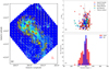 |
Fig. 1 Polarimetric results obtained toward the L1172/1174 cloud complex. (a) R-band (yellow) and Planck (white) polarization vectors (90° rotated) overlaid on the Herschel dust column density map of L1172/1174 obtained from André et al. (2010). The contours are drawn at 9 × 1020 cm−2 and 15 × 1020 cm−2 levels to reveal the cloud structure. HD 200775 is marked with a red star symbol. The dashed red circle represents the head region of the cloud complex. The green colored plus symbols show the locations of L1173 (south), L1172 (middle), and L1174 (north). The lengths and the orientations of the vectors correspondto the degree of polarization and the position angles measured with respect to the Galactic north increasing eastward, respectively. A polarization vector (red) corresponding to 2% and oriented at 90° is shown for reference. (b) Plot of degree of polarization versus position angle values for the 249 sources observed by us in the R band and Planck. The R-band polarization vectors from the head and the tail regions are shown using solid red and blue circles, respectively. Similarly, for Planck, the measurements from the head and the tail regions are shown using solid orange and cyan circles, respectively. The Planck polarization measurements from the ICM are shown with solid gray circles. (c) Histograms of the θR belonging tothe head and the tail regions of L1172/1174 obtained from our R-band polarization measurements with the bin size of ~9°. |
Polarimetric results in head and tail of L1172/1174 and ICM.
3.2 12CO gas distribution in L1172/1174 complex
The 12CO velocity forthe entire cloud complex ranges from −2.8 km s−1 to 7.8 km s−1. The average full width at half maximum (FWHM) of the 12CO is found to be ~2.0 km s−1. The cavity surrounding HD 200775 is conspicuous with high intensity peaks located along the rim of the cavity. The 12CO is found to show gas structures, especially to the east and west of HD 200775, where the gas components in the velocity range of −2.5 –0 km s−1 and 5.0–7.5 km s−1, respectively are located, supporting the earlier reporting of the presence of bipolar outflow lobes (Watt et al. 1986). The Vlsr =2.65 km s−1 of the cloud complex is determined from the N2 H+ line detected in the cores (Sharma et al. 2021, under preparation). The Vlsr is computed as a mean of L1174 (2.5 km s−1) and L1172 (2.8 km s−1) regions. Multiple velocity components in the 12CO line profiles are found in different parts of the cloud complex. The gas dynamics of the region surrounding HD 200775 will be presented in a subsequent article (Sharma et al. 2021, under preparation). In this work, we used the 12CO linewidths to calculate the strength of the BPOS.
4 Discussion
4.1 Magnetic field geometry of the L1172/1174 complex
Interstellar dust grains produce extinction of light from the background stars as well as emit thermal radiation. When the unpolarized starlight impinges on a series of aspherical dust grains, the electromagnetic wave is absorbed maximum along the long axis of grain. The transmitted radiation is parallel to the short axis and becomes partially plane polarized, oriented along the BPOS (Whittet 2005). On the other hand, thermal emission from the dust grains is maximum along the longer axis, thus becomes polarized perpendicular to BPOS. Since dust grains are coupled with the magnetic field, measurements of dust polarization provide information on the structure and the strength of the magnetic field. The value of position angle depends on the orientation of the BPOS and the efficiency of the dust grain alignment with the field. It also depends on the variation in the orientation of BPOS along the line-of-sight (Lee & Draine 1985). The polarization measurements in the optical bands trace the BPOS only in the outskirts of the molecular clouds where the extinction (AV) is relatively low (Guetter & Vrba 1989; Harjunpää et al. 1999). On the other hand, the polarization measurements in submillimeter or millimeter can infer the BPOS inside the cloud where AV is relatively high (e.g., Hildebrand et al. 1984; Goodman 1995; Greaves et al. 1999).
The measured polarization in optical wavelengths is caused by the dust grains that are lying all along the light of sight (within the pencil beam) between the star and us. Though the dust grains present within the cloud are mostly responsible for the observed polarization, those that are present foreground to the cloud can also contribute. To infer the amount of polarization caused by the dust grains within the cloud (thus the magnetic field geometry), it is necessary to remove the foreground component. Generally, the stars located foreground to the cloud are used to estimate the foreground component of the polarization. The PR versus distance and θR versus distance plots of the observed sources are shown in Figs. 3a,b in Saha et al. (2020), respectively,using solid gray triangles (in equitorial coordinate system). The sources having G magnitudes fainter than ~17 were also included in that figure. Among the stars observed by us, only one star, located at 306 pc, is foreground to the cloud. Therefore, we searched in Heiles (2000) catalog to get more foreground sources having polarization measurements. The search was made within a circular region of 6° radius about HD 200775. We obtained a total of 26 sources around HD 200775. In our analysis, we discarded four sources, HD 200775, HD 193533, HD 208947 and HD 203467 (reason for not considering these sources was explained in Saha et al. 2020). Of the remaining 22, we obtained the Gaia DR2 distance for 17 sources from the Bailer-Jones et al. (2018) catalog.
The degree of polarization (PH) in per cent and polarization position angles (θH) in degree of the 17 sources are also shown using filled circles in black in both a and b of Fig. 3 of Saha et al. (2020), respectively.As the foreground sources show significantly low degree of polarization, we set no constraints on the P/σP values during their selection. Of the 17 sources, 13 sources are found to be located at distances less than 335 pc (distance of L1172/1174) and four sources are at distances greater than 335 pc. The mean values of PH and θH for the 13 foreground sources are found to be 0.1% and 122°, respectively and the corresponding mean values for the four background sources are found to be 1.9% and 199°, respectively. Both PH and θH values of the four background sources are found to be consistent with the values of the sources observed by us toward L1172/1174. Using the mean values of PH and θH obtained for the 13 stars, we calculated the mean Stokes parameters Qfg(= Pcos2θ) and Ufg(= Psin2θ) as −0.043 and −0.089, respectively. We subtracted these values from the Stokes parameters of the observed stars vectorially to calculate the foreground-corrected percentage of polarization (Pc) and the position angle (θC) values. No significant changes are noticed in the results after correcting for the foreground polarization. As a result, the R-band polarization vectors (in yellow) presented in Fig. 1a represent the BPOS geometry toward the periphery of L1172/1174 complex.
As evident from Figs. 1a,b, the orientations of BPOS obtained from the R band (θR =203° for the head and θR =196° for the tail) and Planck (θP =212° for the head and θP =200° for the tail) observations are found to be in good agreement all along the structure of the cloud complex. Such correlations between the magnetic field geometries inferred from the optical and the Planck polarization measurements are reported in a number of studies (e.g., Soler et al. 2016; Planck Collaboration Int. XXXV 2016; Gu & Li 2019). This implies that the magnetic fields inferred from the Planck polarization and from the R-band polarization measurements toward the high-density parts and toward the outer envelope of L1172/1174, respectively, are well correlated with each other. Though consistent with the Planck measurements, small-scale substructures in the magnetic field toward the envelope region can be noticed in the R-band polarimetric results. The substructures do not appear in the Planck measurements as Planck traces the large-scale component of the magnetic field. Also, due to the relatively poor resolution, the Planck data could not reveal any effect on the magnetic field by the local kinematics and overall substructures at high-density regimes. Even the Planck polarization vectors from outside of the 9 × 1020 cm−2 contour thatrepresent the BPOS in ICM (θICM =190°) are correlated with both θR and θP implying that the cloud BPOS is threaded by the ICM BPOS surrounding the cloud.
In Fig. 2a we show the BPOS geometry of the head region of L1172/1174 inferred from our R-band and the Planck polarization results. In Figs. 2b,c we show the θR and PR values of the stars as a function of their angular separation from HD 200775, respectively. The Planck polarimetric values (θP and PP) are also shown in the same figures. The primary goal here is to investigate whether the presence of HD 200775 has any effect on the magnetic field geometry around it. Two components of BPOS (θR≥ 196° and < 196°) are apparent in Fig. 2b for the sources lying toward the head region. The changes in the θR and θP found beyond ~ 1° toward the tail are due to the curved geometry of BPOS, which is found to correlate well with the geometry of the cloud structure there. The median values of θR lying toward the head region and having θR ≥ 196° and <196° are found to be 211° and 179° respectively with the MAD of 8° for both the distributions. The distribution of θR in Fig. 2b actually reflects the distribution of the magnetic field vectors on the cloud as shown in Fig. 2a with 179° component lying predominantly to the northwestern parts of HD 200775 and the 211° component lying to the southeastern parts. Similar to Fig. 2b, a clear bimodal angle distribution (θR ≥ 196° and < 196°) of the histogram of θR in head region can be noticed in Fig. 1c. As evident from that figure, the histogram of θR in the tail peaks at the median θR (196°), almost overlapping with the higher θR values (≥196°), which is noticeable in Fig. 2b also. Figure 2c is similar to Fig. 1b, which shows that PP values are similar to the PR values. While we obtained the bimodal distribution both in θP and θR, there is no such bimodality present in PP and PR.
The four observed YSO candidates in Table 2 are all found to be located toward the head region. As evident from Figs. 1b,c, the polarimetric results of all the YSO candidates are found to be consistent with other observed stars. The PR and θR of YSO candidates agree well with the median values of the same in the head region of Table 3, except the θR of star ID 3. However, the latter falls well within the range of θR of the headregion. Except star ID 18 in Table 2, θR of other YSO candidates fall on the group of lower θR (< 196°) values.
To investigate the variation in the projected magnetic field orientations in more detail, we divided the head region into 8 equal sectors drawn within the circular area of 0.4° radius centered at HD 200775 as shown in Fig. 2a. The division of the region is made with respect to the symmetry axis of the outflow cavity believed to have been carved out by HD 200775 (Fuente et al. 1998). The star formation process is ongoing mainly in this circular region. The median values of PR (Col. 2), θR (Col. 3) and the MAD (Col. 4) of the θR for each sector are given in Table 4. The component showing the median value of 211° is dominant toward the sectors 2, 3, and 4, which lie to the south and southeast of HD 200775. The median value of PR for this component is 2.4%. The component showing the median value of 179° is largely distributed toward sectors 7 and 8, which lie to the north of HD 200775. The median value of PR for this component is 1.6%, which is relatively low (~2σ). Sectors 1, 5, and 6 show the presence of both the components. The median value of the θR in these three regions is found to be ~200°, which is roughly the average of the two (179° and 211°) components. The deviation in the θR (ΔθR) is found to be the lowest toward the tail region and highest toward sectors 5 and 6.
In Fig. 3 we show the average 12CO (J = 1–0) line profiles for the eight sectors identified toward the head region. The 12CO lines toward the lines-of-sight of the stars for which we have R-band polarization measurements are used for getting the average profiles. The average 12CO line profile for the tail region is also shown in Fig. 3. The measurements having S∕N ≥ 3 are used for generating the average profiles. The estimated Vlsr (=2.65 km s−1) of the cloud complex is also identified with a vertical line to show the presence of redshfited and blueshfited velocity components in different sectors. The 12CO line toward the tail region is found to be peaking at the Vlsr velocity with a FWHM (ΔV) value of 1.7 km s−1 obtained from a Gaussian fit to the profile. However, the profile shows a line profile skewed to the redder velocities, which is more likely to be due to the presence of high-velocity (both blue- and red-shifted) gas.
The average 12CO line profiles for sectors 3, 4, and 7 are found to be consistent with a Gaussian shape, though presence of high-velocity components are seen toward most of the sectors similar to what we observed toward the tail region. While the line peaks toward sectors 1, 3, 4, and 5 are shifted toward the bluer velocities, the line toward sector 7 shows a shift toward the redder velocity with respect to the Vlsr. Sectors 2 and 6 are found to peak at the Vlsr velocity. The line profiles at sectors 1 and 2 show additional components at bluer velocities, whereas a relatively narrow linewidth with high-velocity wings to the redder velocities are seen for the profile in sector 6. Compared to other sectors, sector 5 shows distinct profile with an additional velocity component to the redder side of the line center having both the peaks with comparable intensity. Thus, for sector 5, we fitted the observed line profile with the two Gaussian components and the linewidth (ΔV ≈ 1.3 km s−1) corresponding to the component closest to the Vlsr is used to estimate the magnetic field strength.
It is observed that the high-velocity gas is not widespread but localized. It is possible that the high-velocity gas present toward, especially, sectors 5 and 6 may be responsible for the disturbance of grain alignment and hence the relatively high ΔθR seen in these two regions where two components of θR (< 196° and ≥ 196°) are present. The symmetry axis of the cavity, believed to be carved out by the outflow from HD 200775 (Fuente et al. 1998), is found to be in a direction almost perpendicular to the magnetic field direction. The cavity located to the northwest of HD 200775 is found to be more extended suggesting that this part is relatively more affected by the star than the southeastern cavity. Presence of high-velocity gas in sector 6 supports this observation. In sector 5 also, the presence of additional velocity components disturbs the surrounding material, which results in a higher dispersion in θR. The additional velocity component is considered to originate from a loop structure close to L1172 (will be discussed in detail in Sharma et al., in prep.). The ΔV values estimated for the lines in all sectors are listed in Table 4.
From Fig. 3, it is evident that a majority of the average 12CO (J = 1–0) line profiles seem to have multiple velocity components, though we selected the outer envelope of the cloud complex (where we carried out the R-band polarimetric study), which is of relatively low density. This arises a possibility of overestimation of 12CO linewidth. It would have been better to use 13CO, which was not available in our study. Though we had C18O data toward this region, but being a high-density gas tracer, we could get emission only in the inner region of the cloud complex, where polarimetric measurements are not available. Therefore, we restrained the linewidth measurements using 12CO only.
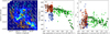 |
Fig. 2 Variation in the projected magnetic field geometry toward the L1172/1174 cloud complex. (a) Optical R-band and Planck polarimetric results overplotted on Herschel column density map. Location of HD 200775 (yellow star) is also shown. The green colored arrows imply the directions of outflow from HD 200775. The eight sectors are indicated using dashed white lines and also marked. Orange lines indicate the polarization measurements in the R band with θR ≥ 196° and cyan lines represent the same with θR < 196°. White lines represent Planck polarimetric results with 90° rotation. A polarization vector corresponding to 2% is shown for reference. (b) Variation in the θR of the sources with respect to the angular separation from HD 200775. Upto 0.4° (Sects. 1–8) there are sources located toward the head region with two sets of distribution of position angles ~211° (red filled circles, shown in orange lines in (a)) and ~179° (blue filled circles, shown in cyan lines in (a)). The green filled circles are the sources distributed toward the tail region. The dashed horizontal line indicates the mean θR value (~ 196°) of the same sources. Position angles obtained from Planck observations are shown using thick open black circles (shown in white lines in (a)). (c) Variation in the PR % and PP % with respectto the angular separation from HD 200775. The symbols represent the same as described in panel b. |
P%, Δθ, ΔV,
 , and BPOS in different sectors of L1172/1174 cloud complex.
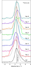 |
Fig. 3 Average 12CO (J = 1–0) line profiles for the eight sectors made toward the head. The average 12CO (J = 1–0) line profile for the tail region is shown in black. The Vlsr =2.65 km s−1 is shown using a dashed vertical line. The dashed curves are the Gaussian fitted lines used to obtain the ΔV. |
4.2 Magnetic field strength in L1172/1174
The strength of the plane-of-sky component of the magnetic field was estimated using the modified Chandrasekhar-Fermi (CF) relation (Chandrasekhar & Fermi 1953; Ostriker et al. 2001),
![\begin{equation*} {B}_{\textrm{POS}} = 9.3 \left[ \frac{{n}_{\textrm{H}_{2}}}{\mathrm{cm}^{-3}} \right]^{1/2} \left[ \frac{\Delta {V}}{\mathrm{km s}^{-1}} \right] \left[\frac{\Delta \theta}{1^{\circ}} \right]^{-1}~~\upmu G,\end{equation*}](/articles/aa/full_html/2021/11/aa39948-20/aa39948-20-eq9.png) (4)
(4)
where  represents the volume density of hydrogen gas in molecular clouds, ΔV is the FWHM obtained from the velocity dispersion σV (
 σV), and Δθ is the dispersion in the position angles. The CF method is applicable for Δθ < 25°. This method suggests that the strength can be estimated by the analysis of small-scale randomness in the magnetic field lines. The line-of-sight velocity dispersion causes an irregular scatter in the polarization position angles under the assumptions that there is a mean field component in the area of interest, that the turbulence responsible for the magnetic field perturbations is isotropic, and that there is equipartition between the turbulent kinetic and magnetic energy (Heitsch et al. 2001). The CF method of estimating BPOS is a statistical method that may be in error by a factor of ~2 for individual clouds.
The observed  is the joint contribution of both the intrinsic dispersion (ΔθR) and measurement uncertainties (
 ) (Lai et al. 2001). Therefore, we obtained the ΔθR using ΔθR =
  ). The
  is the average uncertainty, which was estimated using
  =
=  /N, where
  is the measured uncertainty of the ith star’s polarization angle and N is the total number of stars. The values of ΔV for sectors 1–8 and for the tail, as identified in Fig. 2a, are obtained by fitting Gaussian profiles (single component) to the average 12CO spectrum generated for the individual regions. The estimated values of ΔV are given in the Col. 5 of Table 4. ΔV is the combination of both thermal (ΔVth) and nonthermal (ΔVNT) gas components along the line-of-sight (ΔV =
 ) (Myers 1983). ΔVth can be estimated from
  , where σth is the thermal velocity dispersion of the gas, k is the Boltzmann constant, T is the kinetic temperature and m is molecular weight of the gas. T = 10 K was assumed to estimate the ΔVth in our analysis. We removed the thermal component from the observed linewidth in each sector. The angular extent of the head within the 9 × 1020 cm−2 contour is ~0.6°, which is ~3.5 pc considering its distance as ~335 pc (Saha et al. 2020). For the tail, based on the same contour level, the angular extent was found to be 0.5°, which translates to ~ 2.9 pc at 335 pc. Assuming a similar line-of-sight extent for the cloud and using the hydrogen column density values obtained toward individual stars for which we made R-band polarization measurements, we calculated an average value for
  for each sectors and the tail region. The
  thus obtained are given in Col. 6 of Table 4. The uncertainty in the measurement of
  is taken as 40% of the value (Pokhrel et al. 2016). The BPOS strength calculated for the head and the tail regions are given in Col. 7 of Table 4. The magnetic field strength is found to be weakest in sector 6, which is due to the combined effect of narrow ΔV and relatively high value of ΔθR. The average value of magnetic field strength for the entire cloud is found to be ~30 μG.
4.3 Large-scale magnetic field and bulk motion
Overall, the BPOS geometry in L1172/1174 cloud complex inferred from both the R band and Planck displays an “S” shape morphology with the field lines changing their orientations smoothly as we move from the head to the tail region with BPOS oriented almost parallel to the main filament of the cloud as traced by the 15 × 1020 cm−2 contour as seen in Fig. 1a. In Fig. 4a we show the magnetic field geometry of the region surrounding L1172/1174 and L1147/1158 (1.4° × 1.4°) cloud complexes. The large-scale survey carried out in 13CO (J = 1–0) line of the Cepheus and Cassiopia regions by Yonekura et al. (1997) suggests that both the complexes share similar radial velocities (2.7−2.9 km s−1) implying that the two regions are both spatially and kinematically connected. The distance of 340 ± 3 pc to L1147/1158 estimated using the Gaia DR2 parallax and the proper motion measurements of the YSOs associated with the complex (Sharma et al. 2020) suggests that both L1147/1158 and L1172/1174 are roughly at similar distance from us. At this distance, the spatial separation between the two complexes is ~ 9 pc.
In Fig. 4b we plot PP versus θP from four regions (square boxes of size 0.8° × 0.8°) selected around L1172/1174 cloud complex as shown in Fig. 4a to examine the large-scale magnetic field orientation in the surrounding medium and how it is related to the cloud field lines. The broken lines identify the median values of the two position angle components identified from θR toward the head and the median value of the θR toward the tail as shown in Fig. 2b. The median and MAD values of θP toward L1147/1158 are 182° and 4°, respectively. This is comparable to the 179° component of θR in the northwestern part of the head region of L1172/1174. The θP distribution found toward the regions 1, 2, and 3 resembles the θP distribution found over the whole cloud complex L1172/1174. This is true for both the R band and the Planck polarization results suggesting that the cloud is permeated with the ICM magnetic field. The R-band polarization seems to be consistent with the ICM large-scale magnetic field (derived from Planck) but shows substructures as it follows closely the column density contours (see Fig. 1a). The median values of θP for regions 1–4 are 193° ± 14, 191° ± 5, 175° ± 6, and 135° ± 7, respectively. The θP in regions 1 and 2 are consistent with the median value of θR obtained for the tail region. The median value of 175° obtained for the region 3 is consistent with the 179° component obtained toward sectors 7 and 8 in the head region suggesting that the magnetic field in the head inferred from the R-band polarization measurements is smoothly joining with the ICM field lines inferred from the Planck polarization measurements. The 135° component obtained for the region 4 resembles the change in the magnetic field geometry seen toward the tail part in R-band polarization measurements again suggesting a smooth merger between the cloud and ICM field lines. The θP is found to be relatively scattered in region 1 and in its northeastern part, the alignment of θP is similar to θR of sectors 2 and 3. Globally, regions in the northwest (L1147/1158, L1172/1174, 2, and 3) show θP ~ 180° whereas in the southeastern part (including 1 and 4) θP is highly disturbed.
Based on the Histogram of Relative Orientations analysis (HRO; Soler et al. 2013) with decaying supersonic turbulence, it was shown that in the high-magnetization scenario, the magnetic field changes direction from being parallel to perpendicular with respect to the density structures. The relative orientation becomes random or parallel in the intermediate- or low-magnetization scenario suggesting that the strength of magnetic field may also play a crucial role. The relative orientation is also found to change progressively with increasing column density, from mostly parallel or having no preferred orientation to mostly perpendicular (Planck Collaboration Int. XXXV 2016). Applying HRO analysis, Soler (2019) presented the orientation of BPOS for the Cepheus flare region using the Planck polarization data (Fig. 3: Soler 2019). It was noted that the elongated structure of the cloud complex and BPOS are almost parallel across all the column density values in L1172/1174 cloud complex while they are perpendicular in the L1147/1158 cloud complex, which is clearly visible in Fig. 4a. There is also a marked difference between the magnetic field orientation to the northwestern and southeastern parts of L1172/1174. While the magnetic fields show an almost uni-directional pattern (mostly along 180°) in the northwestern parts of L1172/1174 where L1147/1158 is also located, to the southeastern parts, the magnetic field lines show more twists and turns.
Studies conducted to investigate the relative orientation between the filamentary structure and the magnetic field in a sample of molecularclouds associated with the Gould Belt report a bimodal distribution of the angles between filaments and magnetic fields with the offsets being either parallel or perpendicular (Li et al. 2013; Gu & Li 2019). Results from simulations (Seifried & Walch 2015) and observational studies (Li et al. 2017) suggest that the bimodality may have implications in cloud’s evolution and subsequent star formation process. The molecular clouds with the long axes perpendicular to the magnetic field directions are shown to have more evenly distributed linear mass across the field lines (Law et al. 2019). Also, these clouds consistently show a lower star formation rate (SFR)/mass for clouds (Li et al. 2017). The perpendicular alignment of magnetic field lines possesses a significantly higher flux compared to the parallel orientation and thus provides a stronger support to the molecular clouds against self-gravity (Li et al. 2017). A total of twelve molecular clouds with their SFR/mass and relative orientations of their long axes with magnetic field lines are listed by Li et al. (2017), based on optical and Planck measurements. Of these twelve clouds, six have projected magnetic field aligned perpendicular to the longer axes, while this alignment isparallel for other six clouds. Li et al. (2017) found significant difference in SFR/cloud mass in these two sets of orientations (see Table 5). Our study makes further addition to the findings by Li et al. (2017).
We estimated the SFR in L1172/1174 complex using the total number of YSOs identified toward the cloud and by assuming a mean YSO mass of 0.5 ± 0.1 M⊙ and age of 2 ± 1 Myr (Evans et al. 2009, 2014; Heiderman et al. 2010; Li et al. 2017). A total of 74 YSOs have been identified so far toward L1172/1174 complex (Saha et al. 2020). Based on their positions on the color-magnitude diagram produced using the data from the Gaia DR2, Saha et al. (2020) found an age of ~1–2 Myr for the YSOs, which is consistent with the median age of ~1.6 Myr determined by Kun et al. (2009), and thus, in turn, similar to the age we assumed for the estimation of SFR in this cloud complex. Also, the majority of the sources identified so far in L1172/1174 complex are of low-mass M types (0.1–0.7 M⊙), which is found to be consistent with our assumptions. The SFR thus calculated is found to be 19 ± 10 M⊙ Myr−1. The mass of the cloud was estimated by summing up all those pixels having the hydrogen column density threshold of 9 × 1020 cm−2 (AV ≳ 1.0 magnitude) and using it in the expression M = N(H2)mHμA (Bresnahan et al. 2018), where M is the cloud mass per pixel, N(H2) indicates the H2 column density, mH represents mass of a hydrogen atom, μ = 2.86, the mean particle mass (assuming ~70% H2 by mass), and A represents the area of each pixel. We estimated the area A using (π/180/3600)2 D(cm)2 R(′′)2, where D is the distance to the cloud complex and R(′′) is the size of one pixel. We estimated a cloud mass of 950 ± 380 M⊙. The error is estimated by propagating the uncertainties in the column density estimation and in the distance. Recently, Di Francesco et al. (2020) estimated the mass of L1172/1174 as 1000 M⊙ with AV >1, which is consistent with the mass we obtained. Thus the SFR/mass estimated for L1172/1174 is 2.0 ± 1.3% Myr−1, which is comparable with the mean value 1.98 ± 0.92% Myr−1 obtained by Li et al. (2017), for the clouds with parallel alignments (e.g., Ophiuchus, Corona Australis, Aquila, Perseus etc.). Similarly, we estimated the SFR/mass of the neighboring cloud complex L1147/1158, which has its long axis almost perpendicular to the projected magnetic field direction. Considering the same hydrogen column density threshold (9 × 1020 cm−2) condition, the mass of L1147/1158 is estimated to be 800 ± 320 M⊙, which is consistent with the mass 790 M⊙, obtained by Di Francesco et al. (2020). A total of 14 YSO candidates (Kirk et al. 2009) including PV Cep are distributed within the defined threshold. The SFR is computed as 3.5 ± 1.9 M⊙ Myr−1. Therefore, the estimated SFR/mass for L1147/1158 is 0.4 ± 0.3% Myr−1, which is significantly lower than the same obtained for L1172/1174. But it is consistent with the mean value for the clouds having magnetic field lines perpendicular to their long axes (0.620 ± 0.37% Myr−1; Li et al. 2017). These results further support the claim by Li et al. (2017) that if the magnetic field lines are aligned parallel to the cloud’s long axis (like in L1172/1174, Ophiuchus, Aquila, Perseus etc.), the SFR is found to be higher than in the clouds where the magnetic field lines are aligned perpendicular to the cloud’s long axis (like in L1147/1158, IC 5146, Pipe Nebula, Taurus etc.).
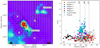 |
Fig. 4 Variation in the projected magnetic field geometry toward L1172/1174 shown in a wider (4° × 4°) area. (a) Magnetic field map (lines in black with white border) of the region covering L1147/1158 and L1172/1174 inferred from the Planck polarization measurements. The magnetic field map of L1172/1174 produced using our R-band polarizationmeasurements are also shown using black lines. (b) Regions from which we obtained Planck polarization measurements shown as boxes (1–4, L1172/1174, and L1147/1158), plotted along with our R-band polarization measurements in L1172/1174. |
SFR per unit cloud mass values (%) of molecular clouds from Li et al. (2017) and from our study.
5 Summary and conclusion
We present the results of our R-band polarization measurements of 249 sources projected on the cloud complex L1172/1174. Combining our results with those from the Planck polarization measurements of the region containing the complex, we studied the magnetic field geometry of the cloud and its relationship with the ICM magnetic field. We summarize the results obtained from this work below:
-
The magnetic field geometry inferred from our R-band polarization measurements and from Planck are found to be in good agreement throughout the cloud. The magnetic field is found to be smooth (not chaotic) and oriented along the hub-filament structure of the cloud. The only changes noticed are toward the extreme ends of the head and the tail regions where the magnetic field lines are found to join smoothly with the ambient magnetic fields in the ICM.
-
Overall, there is not much effect of the presence of HD 200775 on the magnetic field geometry of the surrounding region except toward the northwestern part of HD 200775 where field lines are showing a relatively large dispersion in the magnetic field vectors. The 12CO line profile shows a presence of high-velocity clouds in this region, which may be responsible for disturbing the magnetic field geometry.
-
The mean magnetic field strength for the entire cloud was found to be ~30 μG. Globally, the magnetic field geometry inferred from the Planck polarization is found to be oriented along a mean position angle of 180° toward the northwestern side of L1172/1174 where the cloud complex L1147/1158 is located. At the location of the cloud, the magnetic field lines change to a mean position angle of 200° and then to the southeastern side of L1172/1174, the magnetic field lines show more twists and turns.
-
The higher SFR/mass of 2.0 ± 1.3% Myr−1 found for L1172/1174, compared to 0.4 ± 0.3% Myr−1 for L1147/1158, is consistent with the earlier results, which suggests that the molecular clouds with magnetic field lines oriented parallel to the cloud elongation are found to show relatively high values of SFR compared to those with field lines perpendicular to the cloud elongation.
As a whole, this study helps us to understand the morphology of the projected magnetic field geometry toward the inner high-density as well as the outer low-density regions of the L1172/1174 cloud complex and also its impact in the SFR.
Acknowledgements
We thank Dr. Archana Soam and Neha Sharma, and all the supporting staff at ARIES, Nainital who made these observations possible. C.W.L was supported by the Basic Science Research Program (2019R1A2C1010851) through the National Research Foundation of Korea. T.G. acknowledges support from the Science and Engineering Research Board of the Department of Science and Technology, Govt. of India, grant number SERB/ECR/2018/000826. This work has made use of data from the following sources: (1) the Planck Legacy Archive (PLA) contains all public products originating from the Planck mission, and we take the opportunity to thank ESA/Planck and the Planck collaboration for the same. (2) European Space Agency (ESA) mission Gaia (https://www.cosmos.esa.int/gaia), processed by the Gaia Data Processing and Analysis Consortium (DPAC, https://www.cosmos.esa.int/web/gaia/dpac/consortium). Funding for the DPAC has been provided by national institutions, in particular the institutions participating in the Gaia Multilateral Agreement. This research also has made use of the SIMBAD database, operated at CDS, Strasbourg, France.
Appendix A Table
R-band polarimetric results of 249 stars observed toward L1172/1174.
References
- Alina, D., Ristorcelli, I., Montier, L., et al. 2019, MNRAS, 485, 2825 [Google Scholar]
- Alves, F. O., Franco, G. A. P., & Girart, J. M. 2008, A&A, 486, L13 [NASA ADS] [CrossRef] [EDP Sciences] [Google Scholar]
- André, R., & Kremer, G. M. 2014, ArXiv e-prints [arXiv:1411.6096] [Google Scholar]
- André, P., Men’shchikov, A., Bontemps, S., et al. 2010, A&A, 518, L102 [CrossRef] [EDP Sciences] [Google Scholar]
- Arzoumanian, D., André, P., Didelon, P., et al. 2011, A&A, 529, L6 [NASA ADS] [CrossRef] [EDP Sciences] [Google Scholar]
- Bailer-Jones, C. A. L. 2015, PASP, 127, 994 [Google Scholar]
- Bailer-Jones, C. A. L., Rybizki, J., Fouesneau, M., Mantelet, G., & Andrae, R. 2018, AJ, 156, 58 [Google Scholar]
- Ballesteros-Paredes, J., Klessen, R. S., Mac Low, M. M., & Vazquez-Semadeni, E. 2007, Protostars and Planets V, eds. B. Reipurth, D. Jewitt, & K. Keil (Tucson: University of Arizona Press), 63 [Google Scholar]
- Banerjee, R., Vázquez-Semadeni, E., Hennebelle, P., & Klessen, R. S. 2009, MNRAS, 398, 1082 [NASA ADS] [CrossRef] [Google Scholar]
- Bastien, P. 1982, A&AS, 48, 153 [NASA ADS] [Google Scholar]
- Bastien, P. 1985, ApJS, 59, 277 [NASA ADS] [CrossRef] [Google Scholar]
- Bastien, P., & Landstreet, J. D. 1979, ApJ, 229, L137 [NASA ADS] [CrossRef] [Google Scholar]
- Beattie, J. R., & Federrath, C. 2020, MNRAS, 492, 668 [Google Scholar]
- Bhatt, H. C., & Jain, S. K. 1992, MNRAS, 257, 57 [NASA ADS] [Google Scholar]
- Bohlin, R. C., Savage, B. D., & Drake, J. F. 1978, ApJ, 224, 132 [Google Scholar]
- Bresnahan, D., Ward-Thompson, D., Kirk, J. M., et al. 2018, A&A, 615, A125 [NASA ADS] [CrossRef] [EDP Sciences] [Google Scholar]
- Chandrasekhar, S., & Fermi, E. 1953, ApJ, 118, 113 [Google Scholar]
- Chapman, N. L., Goldsmith, P. F., Pineda, J. L., et al. 2011, ApJ, 741, 21 [NASA ADS] [CrossRef] [Google Scholar]
- Chen, C.-Y., & Ostriker, E. C. 2014, ApJ, 785, 69 [NASA ADS] [CrossRef] [Google Scholar]
- Chen, H.-R. V., Zhang, Q., Wright, M. C. H., et al. 2019, ApJ, 875, 24 [Google Scholar]
- Davis, Jr. L., & Greenstein, J. L. 1951, ApJ, 114, 206 [Google Scholar]
- Di Francesco, J., Keown, J., Fallscheer, C., et al. 2020, ApJ, 904, 172 [NASA ADS] [CrossRef] [Google Scholar]
- Dolginov, A. Z., & Mitrofanov, I. G. 1976, Ap&SS, 43, 291 [NASA ADS] [CrossRef] [Google Scholar]
- Draine, B. T., & Weingartner, J. C. 1996, ApJ, 470, 551 [NASA ADS] [CrossRef] [Google Scholar]
- Draine, B. T., & Weingartner, J. C. 1997, ApJ, 480, 633 [NASA ADS] [CrossRef] [Google Scholar]
- Dutta, S., Mondal, S., Samal, M. R., & Jose, J. 2018, ApJ, 864, 154 [NASA ADS] [CrossRef] [Google Scholar]
- Elsasser, H., & Staude, H. J. 1978, A&A, 70, L3 [NASA ADS] [Google Scholar]
- Eswaraiah, C., Pandey, A. K., Maheswar, G., et al. 2011, MNRAS, 411, 1418 [NASA ADS] [CrossRef] [Google Scholar]
- Eswaraiah, C., Pandey, A. K., Maheswar, G., et al. 2012, MNRAS, 419, 2587 [NASA ADS] [CrossRef] [Google Scholar]
- Eswaraiah, C., Lai, S.-P., Chen, W.-P., et al. 2017, ApJ, 850, 195 [NASA ADS] [CrossRef] [Google Scholar]
- Evans, Neal J., I., Dunham, M. M., Jørgensen, J. K., et al. 2009, ApJS, 181, 321 [NASA ADS] [CrossRef] [Google Scholar]
- Evans, Neal J., I., Heiderman, A., & Vutisalchavakul, N. 2014, ApJ, 782, 114 [CrossRef] [Google Scholar]
- Fiege, J. D., & Pudritz, R. E. 2000, MNRAS, 311, 105 [NASA ADS] [CrossRef] [Google Scholar]
- Franco, G. A. P., Alves, F. O., & Girart, J. M. 2010, ApJ, 723, 146 [Google Scholar]
- Fuente, A., Martin-Pintado, J., Rodriguez-Franco, A., & Moriarty-Schieven, G. D. 1998, A&A, 339, 575 [NASA ADS] [Google Scholar]
- Gaia Collaboration (Brown, A. G. A., et al.) 2018, A&A, 616, A1 [NASA ADS] [CrossRef] [EDP Sciences] [Google Scholar]
- Gold, T. 1952a, Nature, 169, 322 [NASA ADS] [CrossRef] [Google Scholar]
- Gold, T. 1952b, MNRAS, 112, 215 [NASA ADS] [Google Scholar]
- Gómez, G. C., & Vázquez-Semadeni, E. 2014, ApJ, 791, 124 [Google Scholar]
- Gómez, G. C., Vázquez-Semadeni, E., & Zamora-Avilés, M. 2018, MNRAS, 480, 2939 [Google Scholar]
- Goodman, A. A. 1995, ASP Conf. Ser., 73 [Google Scholar]
- Goodman, A. A. 1996, ASP Conf. Ser., 97, 325 [NASA ADS] [Google Scholar]
- Goodman, A. A., Bastien, P., Menard, F., & Myers, P. C. 1990, ApJ, 359, 363 [NASA ADS] [CrossRef] [Google Scholar]
- Goodman, A. A., Jones, T. J., Lada, E. A., & Myers, P. C. 1992, ApJ, 399, 108 [Google Scholar]
- Goodman, A. A., Jones, T. J., Lada, E. A., & Myers, P. C. 1995, ApJ, 448, 748 [NASA ADS] [CrossRef] [Google Scholar]
- Górski, K. M., Hivon, E., Banday, A. J., et al. 2005, ApJ, 622, 759 [Google Scholar]
- Greaves, J. S., Holland, W. S., Minchin, N. R., Murray, A. G., & Stevens, J. A. 1999, A&A, 344, 668 [Google Scholar]
- Gu, Q., & Li, H.-b. 2019, ApJ, 871, L15 [NASA ADS] [CrossRef] [Google Scholar]
- Guetter, H. H., & Vrba, F. J. 1989, AJ, 98, 611 [NASA ADS] [CrossRef] [Google Scholar]
- Hajigholi, M., Persson, C. M., Wirström, E. S., et al. 2016, A&A, 585, A158 [NASA ADS] [CrossRef] [EDP Sciences] [Google Scholar]
- Hall, J. S. 1949, Science, 109, 166 [NASA ADS] [CrossRef] [Google Scholar]
- Hamaker, J. P., & Bregman, J. D. 1996, A&AS, 117, 161 [NASA ADS] [CrossRef] [EDP Sciences] [Google Scholar]
- Harjunpää, P., Kaas, A. A., Carlqvist, P., & Gahm, G. F. 1999, A&A, 349, 912 [NASA ADS] [Google Scholar]
- Hartmann, L., Ballesteros-Paredes, J., & Bergin, E. A. 2001, ApJ, 562, 852 [NASA ADS] [CrossRef] [Google Scholar]
- Heiderman, A., Evans, Neal J., I., Allen, L. E., et al. 2010, ApJ, 723, 1019 [NASA ADS] [CrossRef] [Google Scholar]
- Heiles, C. 2000, AJ, 119, 923 [Google Scholar]
- Heitsch, F., Zweibel, E. G., Mac Low, M.-M., Li, P., & Norman, M. L. 2001, ApJ, 561, 800 [Google Scholar]
- Hennebelle, P. 2013, A&A, 556, A153 [NASA ADS] [CrossRef] [EDP Sciences] [Google Scholar]
- Heyer, M., Goldsmith, P. F., Yıldız, U. A., et al. 2016, MNRAS, 461, 3918 [NASA ADS] [CrossRef] [Google Scholar]
- Hildebrand, R. H., Dragovan, M., & Novak, G. 1984, ApJ, 284, L51 [NASA ADS] [CrossRef] [Google Scholar]
- Hill, T., Motte, F., Didelon, P., et al. 2011, A&A, 533, A94 [NASA ADS] [CrossRef] [EDP Sciences] [Google Scholar]
- Hiltner, W. A. 1949, ApJ, 109, 471 [NASA ADS] [CrossRef] [Google Scholar]
- Iffrig, O., & Hennebelle, P. 2017, A&A, 604, A70 [NASA ADS] [CrossRef] [EDP Sciences] [Google Scholar]
- Inutsuka, S.-i., Inoue, T., Iwasaki, K., & Hosokawa, T. 2015, A&A, 580, A49 [NASA ADS] [CrossRef] [EDP Sciences] [Google Scholar]
- Jiménez-Serra, I., Caselli, P., Fontani, F., et al. 2014, MNRAS, 439, 1996 [Google Scholar]
- Jeong, I.-G., Kang, H., Jung, J., et al. 2019, J. Korean Astron. Soc., 52, 227 [NASA ADS] [Google Scholar]
- Kirk, J. M., Ward-Thompson, D., Di Francesco, J., et al. 2009, ApJS, 185, 198 [NASA ADS] [CrossRef] [Google Scholar]
- Kirk, H., Myers, P. C., Bourke, T. L., et al. 2013, ApJ, 766, 115 [Google Scholar]
- Kirk, H., Klassen, M., Pudritz, R., & Pillsworth, S. 2015, ApJ, 802, 75 [NASA ADS] [CrossRef] [Google Scholar]
- Klessen, R. S., Heitsch, F., & Mac Low, M.-M. 2000, ApJ, 535, 887 [NASA ADS] [CrossRef] [Google Scholar]
- Koch, P. M., Tang, Y.-W., & Ho, P. T. P. 2013, ApJ, 775, 77 [NASA ADS] [CrossRef] [Google Scholar]
- Koch, P. M., Tang, Y.-W., Ho, P. T. P., et al. 2014, ApJ, 797, 99 [NASA ADS] [CrossRef] [Google Scholar]
- Kun, M., Balog, Z., Kenyon, S. J., Mamajek, E. E., & Gutermuth, R. A. 2009, ApJS, 185, 451 [Google Scholar]
- Lada, C. J., Lombardi, M., & Alves, J. F. 2010, ApJ, 724, 687 [Google Scholar]
- Lai, S.-P., Crutcher, R. M., Girart, J. M., & Rao, R. 2001, ApJ, 561, 864 [NASA ADS] [CrossRef] [Google Scholar]
- Law, C. Y., Li, H. B., & Leung, P. K. 2019, MNRAS, 484, 3604 [NASA ADS] [CrossRef] [Google Scholar]
- Lazarian, A., & Hoang, T. 2007, MNRAS, 378, 910 [Google Scholar]
- Lee, H. M., & Draine, B. T. 1985, ApJ, 290, 211 [Google Scholar]
- Li, H.-b., Dowell, C. D., Goodman, A., Hildebrand, R., & Novak, G. 2009, ApJ, 704, 891 [NASA ADS] [CrossRef] [Google Scholar]
- Li, H.-B., Blundell, R., Hedden, A., et al. 2011, MNRAS, 411, 2067 [NASA ADS] [CrossRef] [Google Scholar]
- Li, H.-b., Fang, M., Henning, T., & Kainulainen, J. 2013, MNRAS, 436, 3707 [NASA ADS] [CrossRef] [Google Scholar]
- Li, H. B., Goodman, A., Sridharan, T. K., et al. 2014, in Protostars and Planets VI, eds. H. Beuther, R. S. Klessen, C. P. Dullemond, & T. Henning (Tucson: University of Arizona Press), 101 [Google Scholar]
- Li, H.-B., Jiang, H., Fan, X., Gu, Q., & Zhang, Y. 2017, Nat. Astron., 1, 0158 [NASA ADS] [CrossRef] [Google Scholar]
- Lu, X., Zhang, Q., Liu, H. B., et al. 2018, ApJ, 855, 9 [Google Scholar]
- Luri, X., Brown, A. G. A., Sarro, L. M., et al. 2018, A&A, 616, A9 [NASA ADS] [CrossRef] [EDP Sciences] [Google Scholar]
- Lynds, B. T. 1962, ApJS, 7, 1 [NASA ADS] [CrossRef] [Google Scholar]
- Manoj, P., Bhatt, H. C., Maheswar, G., & Muneer, S. 2006, ApJ, 653, 657 [Google Scholar]
- Matthaeus, W. H., Pouquet, A., Mininni, P. D., Dmitruk, P., & Breech, B. 2008, Phys. Rev. Lett., 100, 085003 [CrossRef] [Google Scholar]
- Matthews, B. C., McPhee, C. A., Fissel, L. M., & Curran, R. L. 2009, ApJS, 182, 143 [NASA ADS] [CrossRef] [Google Scholar]
- Medhi, B. J., Maheswar, G., Pandey, J. C., Kumar, T. S., & Sagar, R. 2008, MNRAS, 388, 105 [NASA ADS] [CrossRef] [Google Scholar]
- Ménard, F. C. 2005, ASP Conf. Ser., 343, 128 [Google Scholar]
- Molina, F. Z., Glover, S. C. O., Federrath, C., & Klessen, R. S. 2012, MNRAS, 423, 2680 [NASA ADS] [CrossRef] [Google Scholar]
- Molinari, S., Swinyard, B., Bally, J., et al. 2010, A&A, 518, L100 [NASA ADS] [CrossRef] [EDP Sciences] [Google Scholar]
- Montier, L., Plaszczynski, S., Levrier, F., et al. 2015, A&A, 574, A135 [NASA ADS] [CrossRef] [EDP Sciences] [Google Scholar]
- Myers, P. C. 1983, ApJ, 270, 105 [Google Scholar]
- Myers, P. C. 2009, ApJ, 700, 1609 [Google Scholar]
- Nagai, T., Inutsuka, S.-i., & Miyama, S. M. 1998, ApJ, 506, 306 [NASA ADS] [CrossRef] [Google Scholar]
- Nakamura, F., & Li, Z.-Y. 2008, ApJ, 687, 354 [NASA ADS] [CrossRef] [Google Scholar]
- Neha, S., Maheswar, G., Soam, A., Lee, C. W., & Tej, A. 2016, A&A, 588, A45 [NASA ADS] [CrossRef] [EDP Sciences] [Google Scholar]
- Neha, S., Maheswar, G., Soam, A., & Lee, C. W. 2018, MNRAS, 476, 4442 [NASA ADS] [CrossRef] [Google Scholar]
- Ostriker, E. C., Stone, J. M., & Gammie, C. F. 2001, ApJ, 546, 980 [Google Scholar]
- Padoan, P., & Nordlund, Å. 2002, ApJ, 576, 870 [NASA ADS] [CrossRef] [Google Scholar]
- Padoan, P., Juvela, M., Goodman, A. A., & Nordlund, Å. 2001, ApJ, 553, 227 [Google Scholar]
- Palmeirim, P., André, P., Kirk, J., et al. 2013, A&A, 550, A38 [NASA ADS] [CrossRef] [EDP Sciences] [Google Scholar]
- Peretto, N., Fuller, G. A., André, P., et al. 2014, A&A, 561, A83 [NASA ADS] [CrossRef] [EDP Sciences] [Google Scholar]
- Pilbratt, G. L., Riedinger, J. R., Passvogel, T., et al. 2010, A&A, 518, L1 [NASA ADS] [CrossRef] [EDP Sciences] [Google Scholar]
- Pillai, T. G. S., Clemens, D. P., Reissl, S., et al. 2020, Nat. Astron., 4, 1195 [Google Scholar]
- Planck Collaboration I. 2014, A&A, 571, A1 [NASA ADS] [CrossRef] [EDP Sciences] [Google Scholar]
- Planck Collaboration I. 2016, A&A, 594, A1 [NASA ADS] [CrossRef] [EDP Sciences] [Google Scholar]
- Planck Collaboration Int. XIX. 2015, A&A, 576, A104 [NASA ADS] [CrossRef] [EDP Sciences] [Google Scholar]
- Planck Collaboration Int. XXX. 2016, A&A, 586, A133 [NASA ADS] [CrossRef] [EDP Sciences] [Google Scholar]
- Planck Collaboration Int. XXXV. 2016, A&A, 586, A138 [NASA ADS] [CrossRef] [EDP Sciences] [Google Scholar]
- Pokhrel, R., Gutermuth, R., Ali, B., et al. 2016, MNRAS, 461, 22 [NASA ADS] [CrossRef] [Google Scholar]
- Qiu, K., Zhang, Q., Menten, K. M., et al. 2014, ApJ, 794, L18 [NASA ADS] [CrossRef] [Google Scholar]
- Ramaprakash, A. N., Gupta, R., Sen, A. K., & Tandon, S. N. 1998, A&AS, 128, 369 [NASA ADS] [CrossRef] [EDP Sciences] [Google Scholar]
- Rautela, B. S., Joshi, G. C., & Pandey, J. C. 2004, Bull. Astron. Soc. India, 32, 159 [NASA ADS] [Google Scholar]
- Rayner, T. S. M., Griffin, M. J., Schneider, N., et al. 2017, A&A, 607, A22 [NASA ADS] [CrossRef] [EDP Sciences] [Google Scholar]
- Rector, T. A.,& Schweiker, H. 2013, AJ, 145, 35 [NASA ADS] [CrossRef] [Google Scholar]
- Saha, P., Gopinathan, M., Kamath, U., et al. 2020, MNRAS, 494, 5851 [NASA ADS] [CrossRef] [Google Scholar]
- Sato, S. 1988, Prog. Theor. Phys. Suppl., 96, 37 [CrossRef] [Google Scholar]
- Sato, S., Tamura, M., Nagata, T., et al. 1988, MNRAS, 230, 321 [NASA ADS] [CrossRef] [Google Scholar]
- Schmidt, G. D., Elston, R., & Lupie, O. L. 1992, AJ, 104, 1563 [Google Scholar]
- Schneider, N., Csengeri, T., Bontemps, S., et al. 2010, A&A, 520, A49 [CrossRef] [EDP Sciences] [Google Scholar]
- Seifried, D., & Walch, S. 2015, MNRAS, 452, 2410 [Google Scholar]
- Sharma, E., Gopinathan, M., Soam, A., et al. 2020, A&A, 639, A133 [NASA ADS] [CrossRef] [EDP Sciences] [Google Scholar]
- Shetty, R., & Ostriker, E. C. 2006, ApJ, 647, 997 [Google Scholar]
- Shimajiri, Y., André, P., Palmeirim, P., et al. 2019, A&A, 623, A16 [NASA ADS] [CrossRef] [EDP Sciences] [Google Scholar]
- Soam, A., Maheswar, G., Bhatt, H. C., Lee, C. W., & Ramaprakash, A. N. 2013, MNRAS, 432, 1502 [NASA ADS] [CrossRef] [Google Scholar]
- Soam, A., Maheswar, G., & Eswaraiah, C. 2014, Ap&SS, 350, 251 [CrossRef] [Google Scholar]
- Soam, A., Kwon, J., Maheswar, G., Tamura, M., & Lee, C. W. 2015a, ApJ, 803, L20 [NASA ADS] [CrossRef] [Google Scholar]
- Soam, A., Maheswar, G., Lee, C. W., et al. 2015b, A&A, 573, A34 [NASA ADS] [CrossRef] [EDP Sciences] [Google Scholar]
- Soam, A., Maheswar, G., Lee, C. W., Neha, S., & Andersson, B.-G. 2017, MNRAS, 465, 559 [NASA ADS] [CrossRef] [Google Scholar]
- Soam, A., Maheswar, G., Lee, C. W., Neha, S., & Kim, K.-T. 2018a, MNRAS, 476, 4782 [Google Scholar]
- Soam, A., Pattle, K., Ward-Thompson, D., et al. 2018b, ApJ, 861, 65 [Google Scholar]
- Soam, A., Lee, C. W., Andersson, B. G., et al. 2019, ApJ, 883, 9 [NASA ADS] [CrossRef] [Google Scholar]
- Soler, J. D. 2019, A&A, 629, A96 [NASA ADS] [CrossRef] [EDP Sciences] [Google Scholar]
- Soler, J. D., & Hennebelle, P. 2017, A&A, 607, A2 [NASA ADS] [CrossRef] [EDP Sciences] [Google Scholar]
- Soler, J. D., Hennebelle, P., Martin, P. G., et al. 2013, ApJ, 774, 128 [Google Scholar]
- Soler, J. D., Alves, F., Boulanger, F., et al. 2016, A&A, 596, A93 [NASA ADS] [CrossRef] [EDP Sciences] [Google Scholar]
- Stone, J. M., Ostriker, E. C., & Gammie, C. F. 1998, ApJ, 508, L99 [Google Scholar]
- Strom, S. E. 1977, IAU Symp., 75, 179 [NASA ADS] [Google Scholar]
- Sugitani, K., Nakamura, F., Tamura, M., et al. 2010, ApJ, 716, 299 [NASA ADS] [CrossRef] [Google Scholar]
- Sugitani, K., Nakamura, F., Watanabe, M., et al. 2011, ApJ, 734, 63 [Google Scholar]
- Tachihara, K., Onishi, T., Mizuno, A., & Fukui, Y. 2002, A&A, 385, 909 [NASA ADS] [CrossRef] [EDP Sciences] [Google Scholar]
- Tamura, M., Hashimoto, J., Kandori, R., et al. 2011, ASP Conf. Ser., 449, 207 [Google Scholar]
- Tazaki, R., Lazarian, A., & Nomura, H. 2017, ApJ, 839, 56 [NASA ADS] [CrossRef] [Google Scholar]
- The, P. S., de Winter, D., & Perez, M. R. 1994, A&AS, 104, 315 [NASA ADS] [Google Scholar]
- Treviño-Morales, S. P., Fuente, A., Sánchez-Monge, Á., et al. 2019, A&A, 629, A81 [NASA ADS] [CrossRef] [EDP Sciences] [Google Scholar]
- Tritsis, A., & Tassis, K. 2016, MNRAS, 462, 3602 [Google Scholar]
- Van Loo, S., Keto, E., & Zhang, Q. 2014, ApJ, 789, 37 [NASA ADS] [CrossRef] [Google Scholar]
- Vink, J. S., Drew, J. E., Harries, T. J., Oudmaijer, R. D., & Unruh, Y. 2005, MNRAS, 359, 1049 [CrossRef] [Google Scholar]
- Vrba, F. J., Strom, S. E., & Strom, K. M. 1976, AJ, 81, 958 [NASA ADS] [CrossRef] [Google Scholar]
- Wardle, J. F. C., & Kronberg, P. P. 1974, ApJ, 194, 249 [Google Scholar]
- Ward-Thompson, D., Kirk, J. M., Crutcher, R. M., et al. 2000, ApJ, 537, L135 [NASA ADS] [CrossRef] [Google Scholar]
- Ward-Thompson, D., Sen, A. K., Kirk, J. M., & Nutter, D. 2009, MNRAS, 398, 394 [NASA ADS] [CrossRef] [Google Scholar]
- Wareing, C. J., Pittard, J. M., Falle, S. A. E. G., & Van Loo, S. 2016, MNRAS, 459, 1803 [NASA ADS] [CrossRef] [Google Scholar]
- Watt, G. D., Burton, W. B., Choe, S. U., & Liszt, H. S. 1986, A&A, 163, 194 [NASA ADS] [Google Scholar]
- Weston, E. B. 1953, AJ, 58, 48 [Google Scholar]
- Whittet, D. C. B. 2005, ASP Conf. Ser., 343, 321 [NASA ADS] [Google Scholar]
- Williams, G. M., Peretto, N., Avison, A., Duarte-Cabral, A., & Fuller, G. A. 2018, A&A, 613, A11 [NASA ADS] [CrossRef] [EDP Sciences] [Google Scholar]
- Wolf, S., Launhardt, R., & Henning, T. 2003, ApJ, 592, 233 [NASA ADS] [CrossRef] [Google Scholar]
- Yonekura, Y., Dobashi, K., Mizuno, A., Ogawa, H., & Fukui, Y. 1997, ApJS, 110, 21 [NASA ADS] [CrossRef] [Google Scholar]
- Yuan, J.-H., Wu, Y., Li, J. Z., Yu, W., & Miller, M. 2013, MNRAS, 429, 954 [NASA ADS] [CrossRef] [Google Scholar]
- Zamora-Avilés, M., Ballesteros-Paredes, J., & Hartmann, L. W. 2017, MNRAS, 472, 647 [Google Scholar]
- Zonca, A., Singer, L., Lenz, D., et al. 2019, J. Open Source Softw., 4, 1298 [Google Scholar]
All Tables
SFR per unit cloud mass values (%) of molecular clouds from Li et al. (2017) and from our study.
All Figures
|
Fig. 1 Polarimetric results obtained toward the L1172/1174 cloud complex. (a) R-band (yellow) and Planck (white) polarization vectors (90° rotated) overlaid on the Herschel dust column density map of L1172/1174 obtained from André et al. (2010). The contours are drawn at 9 × 1020 cm−2 and 15 × 1020 cm−2 levels to reveal the cloud structure. HD 200775 is marked with a red star symbol. The dashed red circle represents the head region of the cloud complex. The green colored plus symbols show the locations of L1173 (south), L1172 (middle), and L1174 (north). The lengths and the orientations of the vectors correspondto the degree of polarization and the position angles measured with respect to the Galactic north increasing eastward, respectively. A polarization vector (red) corresponding to 2% and oriented at 90° is shown for reference. (b) Plot of degree of polarization versus position angle values for the 249 sources observed by us in the R band and Planck. The R-band polarization vectors from the head and the tail regions are shown using solid red and blue circles, respectively. Similarly, for Planck, the measurements from the head and the tail regions are shown using solid orange and cyan circles, respectively. The Planck polarization measurements from the ICM are shown with solid gray circles. (c) Histograms of the θR belonging tothe head and the tail regions of L1172/1174 obtained from our R-band polarization measurements with the bin size of ~9°. |
| In the text | |
|
Fig. 2 Variation in the projected magnetic field geometry toward the L1172/1174 cloud complex. (a) Optical R-band and Planck polarimetric results overplotted on Herschel column density map. Location of HD 200775 (yellow star) is also shown. The green colored arrows imply the directions of outflow from HD 200775. The eight sectors are indicated using dashed white lines and also marked. Orange lines indicate the polarization measurements in the R band with θR ≥ 196° and cyan lines represent the same with θR < 196°. White lines represent Planck polarimetric results with 90° rotation. A polarization vector corresponding to 2% is shown for reference. (b) Variation in the θR of the sources with respect to the angular separation from HD 200775. Upto 0.4° (Sects. 1–8) there are sources located toward the head region with two sets of distribution of position angles ~211° (red filled circles, shown in orange lines in (a)) and ~179° (blue filled circles, shown in cyan lines in (a)). The green filled circles are the sources distributed toward the tail region. The dashed horizontal line indicates the mean θR value (~ 196°) of the same sources. Position angles obtained from Planck observations are shown using thick open black circles (shown in white lines in (a)). (c) Variation in the PR % and PP % with respectto the angular separation from HD 200775. The symbols represent the same as described in panel b. |
| In the text | |
|
Fig. 3 Average 12CO (J = 1–0) line profiles for the eight sectors made toward the head. The average 12CO (J = 1–0) line profile for the tail region is shown in black. The Vlsr =2.65 km s−1 is shown using a dashed vertical line. The dashed curves are the Gaussian fitted lines used to obtain the ΔV. |
| In the text | |
|
Fig. 4 Variation in the projected magnetic field geometry toward L1172/1174 shown in a wider (4° × 4°) area. (a) Magnetic field map (lines in black with white border) of the region covering L1147/1158 and L1172/1174 inferred from the Planck polarization measurements. The magnetic field map of L1172/1174 produced using our R-band polarizationmeasurements are also shown using black lines. (b) Regions from which we obtained Planck polarization measurements shown as boxes (1–4, L1172/1174, and L1147/1158), plotted along with our R-band polarization measurements in L1172/1174. |
| In the text | |
Current usage metrics show cumulative count of Article Views (full-text article views including HTML views, PDF and ePub downloads, according to the available data) and Abstracts Views on Vision4Press platform.
Data correspond to usage on the plateform after 2015. The current usage metrics is available 48-96 hours after online publication and is updated daily on week days.
Initial download of the metrics may take a while.