| Issue |
A&A
Volume 654, October 2021
|
|
|---|---|---|
| Article Number | A2 | |
| Number of page(s) | 16 | |
| Section | The Sun and the Heliosphere | |
| DOI | https://doi.org/10.1051/0004-6361/202140987 | |
| Published online | 01 October 2021 | |
A fast multi-dimensional magnetohydrodynamic formulation of the transition region adaptive conduction (TRAC) method⋆
1
School of Mathematics and Statistics, University of St Andrews, St Andrews, Fife KY16 9SS, UK
2
Department of Physics and Astronomy, George Mason University, Fairfax, VA 22030, USA
3
NASA Goddard Space Flight Center, Greenbelt, MD 20771, USA
e-mail: This email address is being protected from spambots. You need JavaScript enabled to view it.
4
Rosseland Centre for Solar Physics, University of Oslo, PO Box 1029, Blindern, 0315 Oslo, Norway
5
Dipartimento di Fisica & Chimica, Università di Palermo, Piazza del Parlamento 1, 90134 Palermo, Italy
6
INAF-Osservatorio Astronomico di Palermo, Piazza del Parlamento 1, 90134 Palermo, Italy
Received:
2
April
2021
Accepted:
6
June
2021
Abstract
We have demonstrated that the transition region adaptive conduction (TRAC) method permits fast and accurate numerical solutions of the field-aligned hydrodynamic equations, successfully removing the influence of numerical resolution on the coronal density response to impulsive heating. This is achieved by adjusting the parallel thermal conductivity, radiative loss, and heating rates to broaden the transition region (TR), below a global cutoff temperature, so that the steep gradients are spatially resolved even when using coarse numerical grids. Implementing the original 1D formulation of TRAC in multi-dimensional magnetohydrodynamic (MHD) models would require tracing a large number of magnetic field lines at every time step in order to prescribe a global cutoff temperature to each field line. In this paper, we present a highly efficient formulation of the TRAC method for use in multi-dimensional MHD simulations, which does not rely on field line tracing. In the TR, adaptive local cutoff temperatures are used instead of global cutoff temperatures to broaden any unresolved parts of the atmosphere. These local cutoff temperatures are calculated using only local grid cell quantities, enabling the MHD extension of TRAC to efficiently account for the magnetic field evolution, without tracing field lines. Consistent with analytical predictions, we show that this approach successfully preserves the properties of the original TRAC method. In particular, the total radiative losses and heating remain conserved under the MHD formulation. Results from 2D MHD simulations of impulsive heating in unsheared and sheared arcades of coronal loops are also presented. These simulations benchmark the MHD TRAC method against a series of 1D models and demonstrate the versatility and robustness of the method in multi-dimensional magnetic fields. We show, for the first time, that pressure differences, generated during the evaporation phase of impulsive heating events, can produce current layers that are significantly narrower than the transverse energy deposition.
Key words: magnetohydrodynamics (MHD) / Sun: transition region / Sun: corona / Sun: chromosphere / Sun: flares / hydrodynamics
Movies associated to Figs. 4 and 8 are available at https://www.aanda.org
© ESO 2021
1. Introduction
By using multi-dimensional magnetohydrodynamic (MHD) models to study the physics of magnetically closed loops in the solar atmosphere, we have learned a great deal about the storage and release of energy in the corona (see e.g., Reale 2014; Pontin & Hornig 2020). Simulating the plasma response to the heating in such models requires a physical connection between the corona, transition region (TR), and chromosphere in order to account for field-aligned thermal conduction, optically thin radiation, and chromospheric evaporation. These processes control the evolution of the temperature and density of the confined plasma, which determine the brightness of the emission from the coronal loops.
One of the main difficulties encountered when including such additional physics in MHD models is the need to implement a grid that fully resolves the steep gradients in the TR, which are associated with thermal conduction between the corona and chromosphere (e.g., Antiochos & Sturrock 1978; Vesecky et al. 1979). Resolving these gradients in numerical simulations requires very small grid cell widths, typically less than 1 km (Bradshaw & Cargill 2013), which, in turn, acts as a major constraint on the time step, as required for numerical stability. Obtaining this spatial resolution in active-region-sized 3D MHD models poses a serious challenge (e.g., Reid et al. 2018, 2020; Knizhnik et al. 2019; Kohutova et al. 2020), for simulations to be run in a realistic time.
As pointed out by Bradshaw & Cargill (2013), the main consequence of not properly resolving the TR when using the standard Spitzer & Härm (1953, hereafter SH) conduction method is that the resulting coronal density (n) is artificially low. This happens because the downward heat flux is forced to jump across an under-resolved TR to the chromosphere, where the incoming energy is then strongly radiated. Since the emission measure scales with n2, such underestimations in the density can then potentially lead to inaccurate conclusions when numerical predictions are compared with real observational data.
Furthermore, for the case of steady footpoint heating, Johnston et al. (2019) demonstrated that inadequate TR resolution can result in the suppression of the thermal non-equilibrium cycles (Froment et al. 2018; Winebarger et al. 2018; Klimchuk & Luna 2019) that are present when the TR is properly resolved. Similar results were also reported by Zhou et al. (2021) for the formation of prominences (e.g., Antiochos et al. 1999; Xia et al. 2012). Both are examples where the predicted observational signatures are significantly different depending on the size of grid cells used in the TR.
In a recent paper, Johnston & Bradshaw (2019, hereafter JB19) demonstrated that modelling the transition region with the use of an adaptive conduction (TRAC) method successfully removes this influence of numerical resolution on the coronal density response to heating, while maintaining high levels of agreement with fully resolved hydrodynamic (HD) models. When employed with the coarser spatial resolutions, typically achieved in multi-dimensional MHD codes, the TRAC simulations gave peak density errors of less than 5%, whereas without TRAC, in the equivalent coarse resolution simulations, the errors can be as high as 75% (see e.g., Johnston et al. 2017a, 2020, JB19). This is achieved by enforcing adjustments to the parallel thermal conductivity (κ∥(T)), radiative loss (Λ(T)), and heating (Q) rates that are due, in their original form, to Lionello et al. (2009) and Mikić et al. (2013) and were subsequently extended by Johnston et al. (2020). These conditions act to broaden any unresolved parts of the TR, below an adaptive cutoff temperature (Tc), while ensuring that κ∥(T)Λ(T) and κ∥(T)Q(T) give the same function of temperature as for T ≥ Tc. Johnston et al. (2020) showed that modifications of this form allow the TR to be modelled in HD simulations with tractable grid sizes, of order 50 km, because they preserve the energy balance in the TR and conserve the total amount of energy that is delivered to the chromosphere, consistent with fully resolved models.
The natural extension of the original TRAC method, from 1D HD to multi-dimensional MHD, requires the tracing of magnetic field lines at each time step in order to identify the global cutoff temperature that is associated with each field line. Recently, Zhou et al. (2021) proposed such an approach, applying the 1D TRAC method in 2D MHD simulations of prominence formation by using two different field line tracing techniques. However, multi-dimensional implementations of TRAC that employ the original 1D formulation suffer from limitations that are associated with the need to prescribe a global cutoff temperature to individual field lines. In particular, tracing a sufficient number of magnetic field lines at every time step is computationally very time consuming because of the global communication that is required between all of the grid cells in the numerical domain. The outcome is that field line tracing implementations of the TRAC method are unlikely to be practical in 3D MHD simulations of coronal heating, where the energy release is generated self-consistently through the build-up of magnetic energy in the coronal field and subsequent dissipation through magnetic reconnection events (e.g., Hood et al. 2016; Reale et al. 2016; Reid et al. 2018, 2020).
In this paper, we address these shortcomings by presenting an extension of the TRAC method for use in multi-dimensional MHD simulations, without the need to trace magnetic field lines. This is achieved by prescribing an adaptive cutoff temperature local to each grid cell, using only local grid cell quantities. The full details of the MHD TRAC method are described in Sect. 2, where we also show that moving from a global to a local cutoff temperature preserves the properties of the original TRAC method. Section 3 outlines the numerical experiments, and in Sect. 4 we present the results from 2D MHD simulations that model the thermodynamic response to impulsive heating events in unsheared and sheared arcades of coronal loops. The unsheared arcade simulation is used to benchmark the MHD TRAC method against a series of 1D models, while the sheared arcade model demonstrates the performance of the MHD extension of TRAC in a multi-dimensional magnetic field configuration. We conclude with a discussion of the MHD TRAC method in Sect. 5 and present supplementary material in Appendix A.
2. The TRAC method
In Johnston et al. (2020), we presented an extensive description of the TRAC method for the highly efficient numerical integration of the field-aligned HD equations through the computationally demanding TR. The extension of the method to multi-dimensional MHD simulations will be presented in the following subsections.
2.1. MHD model
To model the magnetic field evolution and plasma response to heating, we considered the following set of MHD equations, which include gravitational stratification and an energy equation that incorporates the effects of thermal conduction and optically thin radiation,
 (1)
(1)
 (2)
(2)
 (3)
(3)
 (4)
(4)
 (5)
(5)
Here, ρ is the mass density, v is the velocity, P is the gas pressure, g is the gravitational acceleration, j is the electric current density, B is the magnetic field, Fvisc. represents the viscous force, ϵ = P/(γ − 1)ρ is the specific internal energy density (where γ = 5/3 is the ratio of specific heats), q is the heat flux vector, Qvisc. represents the viscous heating, Q is a heating function that includes uniform background heating and a time-dependent component that can be dependent on position, n is the number density (n = ρ/1.2mp, where mp is the proton mass), Λ(T) is the radiative loss function in an optically thin plasma, which we approximated using the piecewise continuous function defined in Klimchuk et al. (2008), σ is the electrical conductivity, η is the resistivity, kB is the Boltzmann constant and T is the temperature.
We solved the MHD Eqs. (1)–(5) using the Lagrangian Remap (Lare) code described in Arber et al. (2001). Two small shock viscosity terms were included to ensure numerical stability together with a small background viscosity (Reid et al. 2020). These contribute a force, Fvisc., on the right-hand side of the equation of motion (2) and a heating term, Qvisc., to the energy Eq. (3). The thermal conduction model is based on the Braginskii (1965) heat flux in the presence of a magnetic field, where the heat flux vector,
 (6)
(6)
recovers the anisotropic SH parallel thermal conductivity (Spitzer & Härm 1953) in the limit  . Here, κ∥(T) = κ0T5/2 is the SH parallel coefficient of thermal conduction with κ0 = 10−11 Jm−1 K−7/2 s−1 and the perpendicular conductivity is given by
 (7)
(7)
where  is used to approximate the square of the product between the electron gyrofrequency and electron collision time (ωceτe)2, with bmin = 0.1 G used throughout this paper. In the strong field limit, κ⊥(T) is proportional to κ∥(T)/B2 and when
  , we note that the thermal conductivity reduces to isotropic.
Time-splitting methods are used to update thermal conduction and optically thin radiation separately from the advection terms, as discussed in Appendix A of Johnston et al. (2017a). Furthermore, to treat thermal conduction, we use super time stepping methods, as described in Meyer et al. (2012, 2014) and discussed in Appendix B of Johnston et al. (2017a). This time integration strategy is a computational efficient way of dealing with the potentially large difference between the advection (dtadv) and conduction (dtcond) time step restrictions that are required for numerical stability in an explicit numerical scheme, since dtcond ≪ dtadv is typical for coronal plasma evolution.
2.2. The TRAC method: Extension to MHD models
The extension of the TRAC method to multi-dimensional MHD models requires a more sophisticated treatment than the field-aligned HD implementation. The main challenge that needs to be addressed is how the magnetic field evolution modifies the prescription of the adaptive cutoff temperature along a field line. As pointed out by Ruan et al. (2020), continuing with the same approach as JB19 and Johnston et al. (2020) requires the tracking of magnetic field lines and identification of a cutoff temperature, associated with each field line, at each time step of the numerical simulation. However, this approach, which was subsequently pursued by Zhou et al. (2021), is computationally expensive and non-trivial to parallelise with a strong scaling due to the substantial communication required between all of the grid cells in the numerical domain.
Therefore, it is desirable to develop an optimised extension of the TRAC method, for use in MHD simulations, that prescribes an adaptive cutoff temperature local to each grid cell, using only local grid cell quantities. The full details of such an implementation are described next, starting first with the field-aligned HD formulation, followed by the generalisation to multi-dimensional MHD.
2.2.1. Hydrodynamic implementation
To formulate the extension of the TRAC method, we begin with a steady state version of the energy equation that approximates the SH temperature gradient as given by Eq. (8) in Johnston et al. (2020),
![Mathematical equation: $$ \begin{aligned} \dfrac{T}{L_T} \! = \! \! \dfrac{ \! 5k_B J \! \! \pm \! \! \sqrt{ 25k_B^2J^2 \! \! + \! 4\dfrac{\!\kappa _\parallel (T)}{T} \left[ \left( \! \dfrac{\!P\!}{2k_BT\!} \! \right)^{\!\!2} \! \! \Lambda (T) \! - \! Q \right] \! \! } }{2\dfrac{\!\kappa _\parallel (T)}{T}}, \! \! \end{aligned} $$](/articles/aa/full_html/2021/10/aa40987-21/aa40987-21-eq11.gif) (8)
(8)
where
 (9)
(9)
is the temperature length scale, s is the spatial co-ordinate along the magnetic field, J = nv is the mass flux, and v is the velocity parallel to the magnetic field. We note that the positive (negative) root corresponds to an increasing (decreasing) temperature gradient.
The aim is to construct a conductivity model that broadens the TR, giving a new local temperature length scale (LT(s)) that satisfies the minimum resolution criteria of Johnston et al. (2017a,b). This requires that
 (10)
(10)
where LR(s) = Δs is the local grid cell width and δ = 1/2 is a parameter that controls the number of grid cells used to resolve LT(s).
Combining Eqs. (8) and (10), taking the absolute value of the mass flux term (see below) and considering only the positive root (to remove the dependence on sign of the local temperature gradient), we obtain the following expression for a conductivity model that is fitted to resolve the local temperature length scale,
![Mathematical equation: $$ \begin{aligned} \kappa _\parallel ^{\textsc{TRAC}}(T) \! = \! \! \dfrac{ \! 5k_B |J| \! \! + \! \! \sqrt{ 25k_B^2J^2 \! \! + \! 4\dfrac{\!\kappa _\parallel (T)}{T} \left[ \left( \! \dfrac{\!P\!}{2k_BT\!} \! \right)^{\!\!2} \! \! \Lambda (T) \! - \! Q \right] \! \! } }{\dfrac{2\delta }{L_R}} \! , \! \! \! \end{aligned} $$](/articles/aa/full_html/2021/10/aa40987-21/aa40987-21-eq14.gif) (11)
(11)
which we refer to as the TRAC parallel thermal conductivity. We note that Eq. (11) can also be interpreted as the calculation of a local cutoff temperature in each grid cell, using only local grid cell quantities.
As formulated, the TRAC conductivity only exceeds the SH value (κ∥(T)) in grid cells that would be under-resolved with the SH conductivity. That is locations in the TR where LT(s) < LR(s)/δ. On the other hand,  is smaller than the SH value in properly resolved grid cells (e.g., in the corona where LT(s) > LR(s)/δ). This is the case during the evaporation and peak density phases of an impulsively heated loop because the approximation of the SH temperature gradient, used in the calculation of the TRAC conductivity, reduces to the simplified expressions presented in Johnston et al. (2020), for the two limits of strong evaporation (neglecting radiation) and peak density (neglecting mass flux terms). Thus, the TRAC conductivity is calculated using an accurate approximation of the SH temperature gradient, during these first two phases.
We note that it is necessary to take the absolute value of the mass flux term in order to ensure that the TRAC conductivity remains smooth during the evaporation phase, when large upflows in the TR are accompanied by small downflows at the base of the TR (see e.g., Johnston et al. 2020). The evaporation phase is prioritised because this phase has the most severe requirements for resolving the downward heat flux. However, for the decay phase of an impulsively heated loop the mass flux term is negative (downflow). Therefore, the approximation of the temperature gradient used in Eq. (11) does not recover the radiative cooling limit (neglecting thermal conduction) due to the sign enforced by the |J| term. The outcome is that the TRAC conductivity can lead to an over-broadening of the TR during the decay phase.
To mitigate this over-broadening effect, we imposed a limiter on the TRAC conductivity, which is derived by neglecting the mass flux terms,
![Mathematical equation: $$ \begin{aligned} \kappa _\parallel ^{\textsc{LIM}}(T) \! = \dfrac{ \! \! \sqrt{ 4\dfrac{\!\kappa _\parallel (T)}{T} \left[ \left( \! \dfrac{\!P\!}{2k_BT\!} \! \right)^{\!\!2} \! \! \Lambda (T) \! - \! Q \right] \! \! } }{\dfrac{2\delta }{L_R}} \! . \! \! \end{aligned} $$](/articles/aa/full_html/2021/10/aa40987-21/aa40987-21-eq16.gif) (12)
(12)
This limited conductivity is used when grid cells would be under-resolved with the SH conductivity and over-resolved with the TRAC conductivity given by Eq. (11). Such grid cells are regarded as being over-resolved if the new local temperature length scale, given by Eq. (9), is broadened beyond twice the value intended by Eq. (10). Therefore, the threshold for transitioning to  is taken as LT(T) > 2LR(T)/δ.
Incorporating the TRAC conductivity with the broadening limiter, we set the parallel thermal conductivity to be of the form
 (13)
(13)
which increases the conductivity in under-resolved grid cells and reduces to the classical SH value elsewhere, as we show in the next subsection. This calculation of the  conductivity model comprises the first part of the TRAC method as described in JB19.
The second part of the method is to broaden the steep temperature and density gradients in the TR. This is achieved using an approach first proposed by Linker et al. (2001), Lionello et al. (2009) and Mikić et al. (2013).
Using the  conductivity model, we modify the radiative loss rate (Λ(T)) to preserve
  ,
,
 (14)
(14)
and the heating rate (Q(T)) to preserve  ,
,
 (15)
(15)
Reducing both Λ(T) and Q(T), in this way, ensures that the total radiation and heating, integrated across the TR remains the same for both the SH and TRAC methods (Johnston et al. 2020).
2.2.2. Comparison between the SH and TRAC models
Figure 1 shows the outcome of implementing the method outlined above for a loop of total length 60 Mm, in hydrostatic equilibrium with an apex temperature of 1.16 MK. In the upper two panels we focus on the TR, showing the temperature and density as a function of position. An enlargement about the broadened region that uses the TRAC conductivity, referred to as the TRAC region, is also shown inset. In the lower six panels, we show the parallel thermal conductivity, temperature length scale, local radiative losses, local background heating, integrated radiative losses and integrated background heating as functions of temperature. The integrated quantities are defined as being from the apex of the loop downwards to the base of the TR and are shown on a linear scale. In these panels, the solid red and dashed blue lines are the SH and TRAC solutions, respectively. The TRAC (SH) solution is calculated using a grid size of approximately 60 km (60 m). Starting from the left, the first dashed red (blue) vertical line shows the base of the TR for the TRAC (SH) solution, and the next dot-dashed red line the top of the TRAC region. The rightmost vertical dot-dashed blue line is the top of the actual TR, defined by where the downward conduction changes sign from a loss to a gain (e.g., Vesecky et al. 1979; Klimchuk et al. 2008).
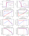 |
Fig. 1. Comparison of the SH and TRAC conduction methods for a one-dimensional loop in hydrostatic equilibrium. Upper two panels: temperature and density as functions of position along the loop. Lower six panels: parallel thermal conductivity, temperature length scale, local radiative losses, local background heating rate, integrated radiative losses, and integrated background heating as functions of temperature. The lines are colour-coded in a way that reflects the conduction method used with dashed blue (solid red) representing the TRAC (SH) solution. The dashed red (blue) vertical line indicates the base of the TRAC (SH) TR and the dot-dashed red (blue) vertical line the temperature at the top of the TRAC region (the temperature at the top of the TR). |
The upper two panels (row 1) show the TR broadening that is associated with the TRAC method, on the temperature and density structure in the lower TR. In particular, the TRAC region extends the TR both below and above the SH location, as was also shown for static loops by Lionello et al. (2009) and dynamic loops in response to heating by Johnston et al. (2020). The third panel demonstrates that the TRAC thermal conductivity is increased relative to the SH value only in under-resolved grid cells and reduces to the SH model elsewhere. This helps to broaden the temperature length scale (fourth panel) in grid cells that would be under-resolved with the SH conduction method. For example, the minimum LT with the TRAC (SH) conduction method is of order 100 km (1 km) for the loop shown in Fig. 1. Thus, the TRAC temperature length scale satisfies the minimum resolution criteria presented in Eq. (10), shown as the lower solid green line in the fourth panel, and the extent of the broadening is bounded by the over-resolution limit described above in Eq. (13) (shown as the upper solid green line). The broadened temperature length scale obtained with TRAC prevents the heat flux from jumping across any unresolved regions while maintaining accuracy in the properly resolved parts of the atmosphere (see e.g., JB19).
The lower four panels of Fig. 1 demonstrate that moving from a global to a local cutoff temperature conserves the properties of the original TRAC method. In particular, consistent with the analytical predictions of Johnston et al. (2020), the TRAC broadening modifications to the local radiative loss and heating rates (row 3), conserve the total radiative losses and total heating (row 4), when integrated over the loop. This preserves the energy balance in the TR and conserves the total amount of energy that is delivered to the chromosphere. The plots also show that the top of the TR is at 0.68 MK while the top of the TRAC region is at 0.17 MK, corresponding to roughly 60% and 15% of the maximum loop temperature, respectively. The thickness of the TRAC region is thus a small fraction of the TR thickness. Therefore, the TRAC method has limited influence on the coronal properties of the loop. The result is that the SH and TRAC temperature and density profiles converge a short distance above the top of the TRAC region.
We also tested this implementation of TRAC on loops that evolve dynamically in response to heating. These simulations show the same fundamental properties as the hydrostatic loop and excellent agreement with Johnston et al. (2020), as discussed further in Appendix A.
2.2.3. Magnetohydrodynamic implementation
Equations (11)–(15) describe the field-aligned formulation of the TRAC method that is used for the multi-dimensional implementation. The extension to MHD requires the generalisation of the mass flux (J), resolution (LR) and temperature length scale (LT) terms to account for the magnetic field evolution. We define the mass flux parallel to the magnetic field as
 (16)
(16)
the field-aligned resolution is given by
 (17)
(17)
where LR = (Δx, Δy, Δz), and the temperature length scale parallel to the magnetic field is defined as
 (18)
(18)
We note that, analogous to the conduction model described in Eq. (6), finite bmin is used here to make the TRAC conductivity isotropic when B = 0. Furthermore, when TRAC is employed in the MHD model, we calculate  in every grid cell and then solve the full set of MHD Eqs. (1)–(5), but with the use of the modified
  , Λ′(T) and Q′(T).
3. Numerical model and experiments
3.1. Unsheared and sheared arcades
To demonstrate the viability of the MHD implementation of TRAC, we consider a 2D coronal arcade given in cylindrical coordinates (R, θ, y) by
 (19)
(19)
where r is the radius and R, B0 and B1 are constants. If B1 = 0 G, then the arcade is unsheared.
In particular, we consider a surface given by r = R and express the azimuthal distance along the unsheared field as x = Rθ, where L = Rπ is the length of a field line. This variable transformation enables the derivatives along the magnetic field to be written in the form
 (20)
(20)
Hence, we can model an arcade of coronal loops using a straight field geometry with a spatially varying gravity, where x is the spatial coordinate along the magnetic field and y represents the transverse direction. The expression for the gravitational acceleration along the field is then given by
 (21)
(21)
For our unsheared arcade model, we take B0 = 100 G and consider a computational domain of dimensions (x, y) = 60 Mm × 2.4 Mm. The numerical grid used to resolve this domain is comprised of 1024 grid points in x (field-aligned direction), while the influence of using low and high resolution in y (cross-field direction) will be examined in Sects. 3.3 and 4.2.
We stratify the initial atmosphere using the broadened, field-aligned temperature and density profiles shown in Fig. 1, which are calculated using the TRAC conduction method and a grid size of approximately 60 km (Nx = 1024) along the field. It is demonstrated in Appendix A that this field-aligned resolution is adequate to fully resolve the TR, when the TRAC method is employed, for all of the simulations presented in this paper. Here, each field line in the arcade starts in static equilibrium and the total length of each field line (L = 60 Mm) includes a 5 Mm chromosphere at the base of each TR. Following Johnston et al. (2017a), the chromosphere is modelled as a mass reservoir with a constant temperature of 104 K, and gravitationally stratified density, while the optically thin radiative losses are reduced to zero to maintain the isothermal temperature (Klimchuk et al. 1987; Bradshaw & Cargill 2013).
To model a sheared arcade we set B1 = 4 G. This tilts the field so that the field lines are no longer aligned with the numerical grid. The initial conditions are adjusted accordingly to ensure the initial state is an equilibrium.
3.2. Non-uniform coronal heating pulse
The effectiveness of the MHD implementation of TRAC is investigated by considering a spatially non-uniform, impulsive coronal heating event, comprised of a short pulse that lasts for a total duration of 60 s, where the energy deposition is localised at the centre of the computational domain. The temporal profile of the heating pulse is triangular with a linear ramp up to the peak heating rate (QH0) followed by a linear decrease, while the field-aligned heating profile is square, confining the energy release to the uppermost 5 Mm located at the apex of the loop, as shown in Fig. 2 (Q(x) at y = 1.2 Mm is displayed in the upper panel as the red curve). However, we note that the coronal response to apex heating is similar to that of uniform heating because thermal conduction is very efficient at coronal temperatures (see e.g., Johnston et al. 2017a,b). Thus, the results presented here are not highly sensitive to the form of heating profile that is used in the field-aligned direction, given that the same total amount of energy is released at a sufficient height above the footpoints of the loop.
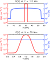 |
Fig. 2. Spatially non-uniform heating profile Q(x, y) (solid red line, left-hand axis) used in Sects. 3 and 4, imposed on top of the temperature initial condition (solid blue line, right-hand axis). Upper (lower) panel: variation of the heating profile in the field-aligned (transverse) direction at the time of peak heating. |
For the transverse direction, the spatial profile of the heating pulse is given by
 (22)
(22)
where QH0 is the maximum heating rate, yH = 100 km is the transverse length scale of heat deposition and we take yL = 1 Mm and yR = 1.4 Mm to give the maximal heating value at y = 1.2 Mm. This is broadly consistent with the spatial distributions of heating reported by Reid et al. (2020). We use a maximum heating rate of QH0 = 8 × 10⁻² Jm−3 s−1, which corresponds roughly to an active region nanoflare (Bradshaw & Cargill 2013).
A small spatially uniform background heating term is also present so that Q(x, y) = Qbg + QH(x, y), where Qbg = 2.2167 × 10⁻⁵ Jm−3 s−1. The initial state of the loop is determined using just Qbg, leading to an apex temperature of 1.16 MK. Defining the transverse heating length scale as
 (23)
(23)
the lower panel of Fig. 2 shows that moving outwards from y = 1.2 Mm, the transverse heating profile decreases smoothly from QH0 to Qbg with a minimum heating length scale of LQy = 50 km.
3.3. One-dimensional simulations of the unsheared arcade
First we solve the unsheared arcade model using a series of 1D field-aligned TRAC simulations that reconstruct the two-dimensional (2D) plasma response to the imposed non-uniform coronal heating pulse. In particular, we treat each field line independently by solving the field-aligned MHD equations with a heating function that is given by the transverse position of the field line in the 2D reconstruction.
The justification for using such an approach is two-fold. Firstly, the 2D reconstruction obtained from the HD simulations will be used as a benchmark solution for comparison with the MHD implementation of TRAC, due to our previous demonstration of excellent agreement with fully resolved field-aligned models (see e.g., JB19, Johnston et al. 2020). Secondly, the results from the 1D simulations also give predictions for the transverse resolution that is required in the MHD model in order to accurately capture all of the features that form in the 2D plasma response.
Figure 3 shows a snapshot at t = 150 s of a number of variables that are reconstructed from the 1D simulations, as a function of the transverse direction (y), at a coronal height of x = 25 Mm. This snapshot corresponds to the time of the first coronal density peak. In the four panels we focus on 0.4 Mm around the centre of the arcade, showing the temperature, density, pressure and field-aligned velocity (vx). Each quantity is shown imposed on top of the transverse heating profile (Q(y)), which is displayed as the red curve. In these panels, the solid blue and dashed green lines are 2D reconstructions that are calculated from the 1D simulations using Ny = 1024 and Ny = 64 grid points in the transverse direction, respectively. These transverse resolutions correspond to grid cell widths of approximately 2.3 km (solid blue curve) and 37.5 km (dashed green curve) in the 2D reconstructions, enabling both grids to fully resolve the minimum transverse heating length scale given by Eq. (23).
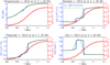 |
Fig. 3. Results for the reconstruction of the non-uniform coronal heating pulse using one-dimensional HD simulations of the unsheared arcade (Sect. 3.3). The panels show the temperature, density, pressure, and field-aligned velocity as functions of position across the arcade (left-hand axis), at a coronal height of x = 25 Mm, at the time of the first density peak (t = 150 s). The lines are colour coded in a way that reflects the transverse resolution used with solid blue (dashed green) representing the Ny = 1024 (Ny = 64) solution, which is imposed on top of the transverse heating profile (solid red line, right-hand axis). |
Starting with the temperature structure across the arcade, it is clear that the transverse variations in the temperature are consistent with the imposed heating function. This happens because the initial temperature evolution is being set by the direct in situ heating. Consequently, the temperature profiles calculated using Ny = 1024 and Ny = 64 grid points show good agreement as both solutions adequately resolve the resultant transverse temperature length scale.
On the other hand, it is striking that the transverse variations in the density have significantly shorter length scales than the heating profile. The minimum transverse density length scale (defined in the same was as the minimum transverse heating length scale) is of order 10 km, which is five times smaller than that of the heating function. Therefore, the density profiles show major differences between low (Ny = 64) and high (Ny = 1024) transverse resolution because the Ny = 64 grid is unable to resolve the narrow transverse variations that are observed with the Ny = 1024 solution.
The generation of these small length scales can be attributed to the coronal density evolution relying on the interplay in the TR between downward conduction and upward enthalpy, entangling the scaling with the imposed heating function (as discussed in detail in Sect. 4.1.1). This is also the case for the pressure, which shows small length scales that are of similar order to those seen in the density, with steep transverse gradients forming around y = 0.93 and y = 1.01 Mm.
Furthermore, the field-aligned velocity across the arcade shows the formation of two shear flow layers that are co-spatial with the steep transverse density and pressure gradients. However, the length scales that are associated with these shear flows are of order 1 km, making it more challenging to resolve the transverse variations in the field-aligned velocity than the density and pressure. The outcome is that there is considerable departure between the velocity profiles calculated using Ny = 1024 and Ny = 64 grid points, with the low resolution solution significantly under-resolving the shear flow layers. Therefore, based on the predictions of the length scales that result in the HD simulations, the MHD model will be run with a transverse resolution of 2.3 km (Ny = 1024), so that the steepness of the shear flow layers is captured reasonably well.
4. Results: Two-dimensional simulations
4.1. Unsheared arcade
Figure 4 summarises the temporal evolution of the MHD simulation of the unsheared arcade, in response to the non-uniform coronal heating pulse. The three columns show contour plots of the temperature, density and field-aligned velocity (vx). Each row shows a snapshot at a different time: t = 10 s (row 1), t = 60 s (row 2), t = 150 s (row 3) and t = 1000 s (row 4). These correspond to times during the heating phase, at the start of the evaporation phase, at the first coronal density peak, and during the arcade’s draining phase, respectively. The black curves on the contour plots show the top of the TRAC region on each of the field lines in the unsheared arcade.
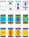 |
Fig. 4. Results for the non-uniform coronal heating pulse using a two-dimensional MHD simulation of the unsheared arcade (Sect. 4.1). Starting from the left, the columns show time ordered snapshots of the temperature (T), density (n) and field-aligned velocity (vx) for times during the heating, evaporation and decay phases. The contours are drawn according to the scales shown in the colour tables. The black curves indicate the top of the TRAC region at each of the footpoints of the unsheared arcade. Movies of the full time evolution of the T, n and vx contour plots can be viewed online. |
Individual field lines located inside the heated region follow an evolution characteristic of an impulsively heated loop (see e.g., Bradshaw & Cargill 2006; Klimchuk 2006; Klimchuk et al. 2008; Cargill et al. 2012a,b, 2015; Reale 2016). For such an evolution, the field-aligned flows associated with the draining phase are typically an order of magnitude smaller than during the evaporation phase (JB19, Johnston et al. 2020). Thus, the scale used for the colour table of the field-aligned velocity in Fig. 4, has been adjusted accordingly, to give an accessible range for the snapshot at t = 1000 s.
4.1.1. Shear flow formation
The collective evolution of the individual field lines leads to the formation of a shear flow layer across the arcade, as shown in Fig. 4. As only a small part of the corona is heated, this initially produces a region with high temperature and pressure. The high pressure causes a downflow, which pushes plasma out of the corona towards the footpoints, while the high temperature causes a conduction front to propagate downwards along the magnetic field, driving a heat flux into the TR.
While the conduction front on a particular field line propagates ahead of the flows generated by the pressure gradient, the speed of the conduction front depends on the temperature reached, which depends on the transverse heating profile. As the conduction front propagates downwards, the plasma lower in the corona is unable to radiate the excess conductive heating and so the gas pressure increases locally. The conduction front then slows down as it reaches the TR and the accompanying increased gas pressure piles up at the base of the TR. This creates an upward pressure gradient that drives an upflow of dense material from the TR to the corona, increasing the coronal density.
However, the timing of this upward pressure gradient depends on the amount of heating in the corona, which depends on the transverse position of the field line. Therefore, a shear flow occurs between strongly and weakly heated regions when there are transverse variations in the energy deposition. This shear flow formation is seen clearly at t = 60 s in the field-aligned velocity plot shown in Fig. 4. Furthermore, row 3 of Fig. 4 demonstrates that the shear flow remains present at the time of the first coronal density peak (t = 150 s). This corresponds to a time when the evaporation fronts on strongly heated field lines have rebounded at the apex and subsequently reversed, transporting the evaporated plasma back towards the footpoints, while the flows on weakly heated field lines are still evaporating mass upwards into the corona. The flows associated with the directly heated plasma do not show such short length scales across the arcade.
4.1.2. Comparison between the HD and MHD models
Figures 5 and 6 compare the response of the 2D MHD model with the results from the 1D HD reconstruction of the unsheared arcade. Hereafter, we refer to these simulations as the MHD and HD TRAC models, respectively. Starting with the coronal response, the two panels in Fig. 5 show the time evolution of the coronal averaged temperature and density, for both models, at four different transverse positions inside the heated region. The coronal averages are calculated by spatially averaging over the uppermost 50% of each field line. Each solid curve represents the particular coronal average on the selected field lines from the HD TRAC reconstruction and the dashed blue curves imposed on top are the corresponding averages from the MHD TRAC simulation.
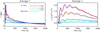 |
Fig. 5. Comparison of the coronal evolution obtained from the two different models of the unsheared arcade (Sect. 4.1), in response to the non-uniform coronal heating pulse. The panels show the coronal averaged temperature and density as functions of time, at four different positions across the magnetic field. The various solid curves represent the HD TRAC solution at these different transverse locations (with the lines colour coded in a way that reflects the distance across the field from the centre of the arcade) and the dashed blue curves correspond to the MHD TRAC solution at these locations. |
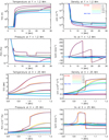 |
Fig. 6. Comparison of the field-aligned and transverse temporal evolution obtained from the two different models of the unsheared arcade (Sect. 4.1), in response to the non-uniform coronal heating pulse. Upper (lower) four panels: time ordered snapshots of the temperature, density, pressure and field-aligned velocity as functions of position along (across) the magnetic field at y = 1.2 Mm (x = 25 Mm). The various solid curves represent the HD TRAC solution at different times (with the lines colour coded in a way that reflects the temporal evolution) and the dashed blue curves correspond to the MHD TRAC solution at these times. |
Both models show excellent agreement across each of the field lines, with a rapid rise in temperature, followed by an increase in density due to evaporation, then, after the time of maximum density, a radiative cooling and draining phase (Bradshaw & Cargill 2010a,b). The density oscillations that are typical for the short heating pulse imposed (e.g., Reale 2016), are damped slightly faster in the MHD model, but the resulting differences are sufficiently small so that the correct draining rate is retained during the decay phase. Therefore, Fig. 5 demonstrates that the MHD code, with the multi-dimensional TRAC method, accurately captures the enthalpy exchange between the corona and TR, through all phases of an impulsive heating event.
This conclusion is confirmed by the temporal comparisons that are presented in Fig. 6. In the upper four panels, we focus on the field-aligned evolution of the unsheared arcade at y = 1.2 Mm, showing the temperature, density, pressure and field-aligned velocity as functions of position along the magnetic field. In the lower four panels, we show the transverse evolution of the same quantities at x = 25 Mm, which is consistent with the coronal height considered previously in Fig. 3. In these panels, using the same line styles as before, each solid curve represents a different snapshot from the HD TRAC model and the dashed blue curves imposed on top are the corresponding snapshots from the MHD TRAC simulation.
First we examine the field-aligned evolution. The third panel of Fig. 6 shows the high level of agreement between the HD and MHD TRAC models, for the evolution of the pressure gradients that form along the field. These pressure gradients subsequently drive the field-aligned flows. It therefore follows that the MHD TRAC solution correctly models the evolution of the field-aligned flows, throughout the evaporation and draining cycle, and this is confirmed in the fourth panel. The outcome is that the mass and energy exchange between chromosphere, TR, and corona is correctly captured by the MHD implementation of TRAC, which, in turn, ensures accuracy in simulating the coronal temperature and density evolution.
Next we look at the transverse evolution. As shown in the fifth panel of Fig. 6, the temperature structure across the arcade shows excellent agreement between the HD and MHD TRAC models, for each of the snapshots. Likewise, the evolution of the transverse variations in the density and pressure shows good agreement between the two models. However, there are some small differences. For example, while the steep transverse density and pressure gradients that form around y = 1.01 Mm, at the time of the first coronal density peak (t = 150 s, orange curve), are accurately captured by the MHD TRAC solution, the accompanying gradients that form further out, around y = 0.93 Mm, are slightly smoothed over by the MHD TRAC model.
Consequently, the MHD TRAC solution correctly models the shear flow layer in the field-aligned velocity that is co-spatial with the transverse gradients at y = 1.01 Mm, but slightly broadens the outer layer at y = 0.93 Mm. Thereafter, minor differences remain for the evolution of the transverse density and pressure structure in the heated region, before both models reconcile later in the decay phase. Overall, Fig. 6 shows that the TRAC method can be used to model the coronal plasma evolution with confidence in multi-dimensional MHD simulations.
4.1.3. MHD effects
Finally, the first panel of Fig. 7 shows that there is a modification to the magnetic field in the MHD simulation in order to keep the total pressure constant in the transverse direction. The second panel shows that this introduces a narrow current layer, which is co-spatial with the shear flow region that forms at y = 1.01 Mm, for the snapshot shown at t = 150 s. We note that this narrow current sheet is fundamentally different from a tangential discontinuity as proposed by Parker (1972) because it is driven by pressure differences instead of constant pressure across a tangentially discontinuous flux surface. Hence, this demonstrates for the first time that the thermodynamic response to spatially non-uniform heating events can generate small transverse length scales in the form of pressure driven current sheets, which are significantly shorter than those that are associated with the heating profile or mechanism.
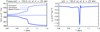 |
Fig. 7. Quantities from the MHD model of the unsheared arcade (Sect. 4.1), at a coronal height of x = 25 Mm, at the time of the first density peak (t = 150 s). Left-hand panel: gas pressure (dashed line), magnetic pressure (solid line), and total pressure (dash-dotted line) as functions of position across the arcade. We note that the gas pressure has been offset by 398.4 × 10⁻¹ Pa in the pressure plot. Right-hand panel: jz component of the current current density. |
4.2. Sheared arcade
Figure 8 shows the outcome of imposing the non-uniform coronal heating pulse in the sheared arcade model, in the same format as Fig. 4. The temporal evolution shows the same fundamental properties as the unsheared arcade, but with the TRAC region and thermodynamic response aligning with the tilted magnetic field accordingly. In particular, we see the formation of a shear flow layer between strongly and weakly heated field lines at the start of the evaporation phase (t = 60 s), which remains prominent at the time of the first coronal density peak (t = 150 s). Therefore, the shear flow is a signature of the evaporated plasma, which is not observed in the directly heated material.
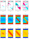 |
Fig. 8. Results for the non-uniform coronal heating pulse using a two-dimensional MHD simulation of the sheared arcade (Sect. 4.2). Notation is the same as that in Fig. 4. Movies of the full time evolution of the T, n and vb contour plots can be viewed online. |
We note that the simulation presented in Fig. 8 used a transverse resolution of 2.3 km (Ny = 1024) in order to resolve the resulting shear flow layer. However, such high spatial resolution across the magnetic field is not typically achieved in active region sized 3D MHD models. Thus, to study the influence of transverse resolution on the shear flow formation, we repeated the sheared arcade simulation using intermediate (Ny = 256) and low (Ny = 64) levels of transverse resolution.
Figure 9 contrasts the results with the shear flow formed in the high resolution simulation at t = 150 s, showing the temperature, density, pressure and velocity parallel to the magnetic field, as functions of position across the sheared arcade. The low (dashed green) and intermediate (dashed red) transverse resolution simulations both show broadened temperature, density and pressure profiles that smooth over the transverse gradients of the high resolution simulation (solid blue). Consistent with numerical diffusion artificially influencing the evolution (due to the finite grid), more significant broadening is associated with lower transverse resolution. This broadening makes it increasingly difficult to detect any local signatures of the shear flow when using lower transverse resolution.
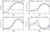 |
Fig. 9. Results for the non-uniform coronal heating pulse released in MHD simulations of the sheared arcade (Sect. 4.2), run with different levels of transverse resolution. The panels show the temperature, density, pressure and velocity parallel to the magnetic field (vb) as functions of position across the arcade, at a coronal height of x = 25 Mm, at the time of the first density peak (t = 150 s). The lines are colour coded in a way that reflects the transverse resolution used with solid blue representing the Ny = 1024 solution and dashed red (dashed green) corresponding to Ny = 256 (Ny = 64). |
However, Fig. 10 demonstrates that this has little effect on the global evolution of the corona because the evaporative response to heating is dominated by the field-aligned mass and energy exchange that takes place between the chromosphere, TR, and corona. A process which is modelled accurately by the TRAC method for each of the different levels of transverse resolution. The outcome is that the coronal averaged temperature and density show good agreement between the high (Ny = 1024), intermediate (Ny = 256) and low (Ny = 64) transverse resolution simulations of the sheared arcade. Therefore, lower transverse resolution does not lead to erroneous conclusions for the coronal plasma evolution when using the MHD implementation of TRAC.
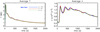 |
Fig. 10. Comparison of the coronal evolution obtained from the sheared arcade simultaions run with different levels of transverse resolution (Sect. 4.2). The panels show the coronal averaged temperature and density as functions of time, where the spatial average was calculated in both x and y over the uppermost 25% of the computational domain. The lines are colour coded in the same way as Fig. 9. |
5. Discussion and conclusions
This paper extends the work of JB19 and Johnston et al. (2020), presenting a highly efficient formulation of the TRAC method for use in multi-dimensional MHD simulations. Extending the TRAC method to MHD has required optimisation in order to efficiently account for the magnetic field evolution, without the need to trace field lines at each time step. In particular, to move from one-dimensional HD to multi-dimensional MHD, we have modified the method from requiring the calculation of a global cutoff temperature that is associated with individual field lines, to employing a local cutoff temperature that is calculated using only local grid cell quantities. However, despite this change from using a global to a local cutoff temperature for broadening the steep gradients in the TR, the total radiative losses and heating remain conserved under the MHD formulation. The outcome is that multi-dimensional MHD simulations using the MHD extension of the TRAC method can accurately model the coronal plasma evolution through all phases of an impulsive heating event.
The advantages of using this novel extension of the TRAC method over field line tracing approaches (see e.g., Zhou et al. 2021) are multiple. For multi-dimensional MHD models, the ability to side-step the need to trace magnetic field lines when applying the MHD TRAC method means that (1) the implementation of the method is substantially simpler, (2) the cutoff temperatures are calculated significantly faster at a fraction of the computational cost, (3) it is fundamentally easier to account for changes in field line connectivity, permitting the plasma response to be modelled accurately with relative ease in coronal heating simulations where the energy release is generated self-consistently through magnetic reconnection events (e.g., Hood et al. 2016; Reale et al. 2016; Reid et al. 2018, 2020) and (4) the method is more readily employed in large-scale 3D MHD simulations, which have more realistic and complex magnetic field configurations (e.g., Warnecke et al. 2017; Mikić et al. 2018; Martínez-Sykora et al. 2018; Knizhnik et al. 2019; Howson et al. 2019, 2020; Kohutova et al. 2020; Antolin et al. 2021). Furthermore, the MHD TRAC method only increases the thermal conductivity relative to the SH value in under-resolved grid cells, while reducing to the SH model elsewhere. Therefore, the method automatically switches off in properly resolved parts of the atmosphere.
While the MHD TRAC method successfully removes the influence of under-resolving the TR on the coronal density response to heating, the broadening modifications act only in the field-aligned direction. This means that full numerical resolution is still required in the transverse direction in order to resolve the current sheets that are responsible for the heating (see e.g., Leake et al. 2020). Moreover, in this paper, we have demonstrated that the evaporative response to impulsive heating events can generate transverse length scales that are much smaller than those associated with the heating mechanism. In particular, we presented the formation of a shear flow, which we identified as a unique signature of the evaporated plasma because such shortened length scales are not observed in the directly heated material, and associated pressure driven current sheets.
In summary, the MHD TRAC method efficiently addresses the difficulty of obtaining the correct evaporative response to impulsive heating events in multi-dimensional MHD simulations, without the need for high spatial resolution in the TR. Indeed, our results suggest that high levels of accuracy can be obtained with grid cell widths of order 50 km in the field-aligned direction, which is achievable in current three-dimensional MHD models. Therefore, the method helps to free up computational resources to better resolve the heating mechanism and subsequent shear flow dynamics. Furthermore, the MHD TRAC method is simple to implement, fast to run and is easily employed in MHD simulations of coronal heating that study the build-up of magnetic energy in complex field configurations and subsequent dissipation through magnetic reconnection.
Movies
Movie 1 associated with Fig. 4 (Fig_4_n_Unsheared_Arcade) Access Supplementary Material
Movie 2 associated with Fig. 4 (Fig_4_T_Unsheared_Arcade) Access Supplementary Material
Movie 3 associated with Fig. 4 (Fig_4_vx_Unsheared_Arcade) Access Supplementary Material
Movie 4 associated with Fig. 8 (Fig_8_n_Sheared_Arcade) Access Supplementary Material
Movie 5 associated with Fig. 8 (Fig_8_T_Sheared_Arcade) Access Supplementary Material
Movie 6 associated with Fig. 8 (Fig_8_vb_Sheared_Arcade) Access Supplementary Material
Acknowledgments
The research leading to these results has received funding from the UK Science and Technology Facilities Council (consolidated grant ST/N000609/1), the European Union Horizon 2020 research and innovation programme (grant agreement No. 647214). IDM received funding from the Research Council of Norway through its Centres of Excellence scheme, project number 262622. CDJ acknowledges support from the International Space Science Institute (ISSI), Bern, Switzerland to the International Teams on “Observed Multi-Scale Variability of Coronal Loops as a Probe of Coronal Heating” and “Interrogating Field-Aligned Solar Flare Models: Comparing, Contrasting and Improving”. We also acknowledge very helpful comments from the referee, Dr. Philip Judge. This work used the DiRAC Data Analytic system at the University of Cambridge, operated by the University of Cambridge High Performance Computing Service on behalf of the STFC DiRAC HPC Facility (www.dirac.ac.uk). This equipment was funded by BIS National E-infrastructure capital grant (ST/K001590/1), STFC capital grants ST/H008861/1 and ST/H00887X/1, and STFC DiRAC Operations grant ST/K00333X/1. DiRAC is part of the National e-Infrastructure.
References
- Antiochos, S. K., & Sturrock, P. A. 1978, ApJ, 220, 1137 [NASA ADS] [CrossRef] [Google Scholar]
- Antiochos, S. K., MacNeice, P. J., Spicer, D. S., & Klimchuk, J. A. 1999, ApJ, 512, 985 [NASA ADS] [CrossRef] [Google Scholar]
- Antolin, P., Pagano, P., Testa, P., Petralia, A., & Reale, F. 2021, Nat. Astron., 5, 54 [NASA ADS] [CrossRef] [Google Scholar]
- Arber, T. D., Longbottom, A. W., Gerrard, C. L., & Milne, A. M. 2001, J. Comput. Phys., 171, 151 [NASA ADS] [CrossRef] [Google Scholar]
- Bradshaw, S. J., & Cargill, P. J. 2006, A&A, 458, 987 [NASA ADS] [CrossRef] [EDP Sciences] [Google Scholar]
- Bradshaw, S. J., & Cargill, P. J. 2010a, ApJ, 710, L39 [NASA ADS] [CrossRef] [Google Scholar]
- Bradshaw, S. J., & Cargill, P. J. 2010b, ApJ, 717, 163 [NASA ADS] [CrossRef] [Google Scholar]
- Bradshaw, S. J., & Cargill, P. J. 2013, ApJ, 770, 12 [NASA ADS] [CrossRef] [Google Scholar]
- Braginskii, S. I. 1965, Rev. Plasma Phys., 1, 205 [Google Scholar]
- Cargill, P. J., Bradshaw, S. J., & Klimchuk, J. A. 2012a, ApJ, 752, 161 [NASA ADS] [CrossRef] [Google Scholar]
- Cargill, P. J., Bradshaw, S. J., & Klimchuk, J. A. 2012b, ApJ, 758, 5 [NASA ADS] [CrossRef] [Google Scholar]
- Cargill, P. J., Warren, H. P., & Bradshaw, S. J. 2015, Philos. Trans. Royal Soc. London Ser. A, 373, 20140260 [NASA ADS] [Google Scholar]
- Froment, C., Auchère, F., Mikić, Z., et al. 2018, ApJ, 855, 52 [Google Scholar]
- Hood, A. W., Cargill, P. J., Browning, P. K., & Tam, K. V. 2016, ApJ, 817, 5 [NASA ADS] [CrossRef] [Google Scholar]
- Howson, T. A., De Moortel, I., Reid, J., & Hood, A. W. 2019, A&A, 629, A60 [NASA ADS] [CrossRef] [EDP Sciences] [Google Scholar]
- Howson, T. A., De Moortel, I., & Reid, J. 2020, A&A, 636, A40 [CrossRef] [EDP Sciences] [Google Scholar]
- Johnston, C. D., & Bradshaw, S. J. 2019, ApJ, 873, L22 [NASA ADS] [CrossRef] [Google Scholar]
- Johnston, C. D., Hood, A. W., Cargill, P. J., & De Moortel, I. 2017a, A&A, 597, A81 [NASA ADS] [CrossRef] [EDP Sciences] [Google Scholar]
- Johnston, C. D., Hood, A. W., Cargill, P. J., & De Moortel, I. 2017b, A&A, 605, A8 [NASA ADS] [CrossRef] [EDP Sciences] [Google Scholar]
- Johnston, C. D., Cargill, P. J., Antolin, P., et al. 2019, A&A, 625, A149 [NASA ADS] [CrossRef] [EDP Sciences] [Google Scholar]
- Johnston, C. D., Cargill, P. J., Hood, A. W., et al. 2020, A&A, 635, A168 [NASA ADS] [CrossRef] [EDP Sciences] [Google Scholar]
- Klimchuk, J. A. 2006, Sol. Phys., 234, 41 [NASA ADS] [CrossRef] [Google Scholar]
- Klimchuk, J. A., & Luna, M. 2019, ApJ, 884, 68 [NASA ADS] [CrossRef] [Google Scholar]
- Klimchuk, J. A., Antiochos, S. K., & Mariska, J. T. 1987, ApJ, 320, 409 [NASA ADS] [CrossRef] [Google Scholar]
- Klimchuk, J. A., Patsourakos, S., & Cargill, P. J. 2008, ApJ, 682, 1351 [Google Scholar]
- Knizhnik, K. J., Antiochos, S. K., Klimchuk, J. A., & DeVore, C. R. 2019, ApJ, 883, 26 [NASA ADS] [CrossRef] [Google Scholar]
- Kohutova, P., Antolin, P., Popovas, A., Szydlarski, M., & Hansteen, V. H. 2020, A&A, 639, A20 [EDP Sciences] [Google Scholar]
- Leake, J. E., Daldorff, L. K. S., & Klimchuk, J. A. 2020, ApJ, 891, 62 [NASA ADS] [CrossRef] [Google Scholar]
- Linker, J. A., Lionello, R., Mikić, Z., & Amari, T. 2001, J. Geophys. Res., 106, 25165 [NASA ADS] [CrossRef] [Google Scholar]
- Lionello, R., Linker, J. A., & Mikić, Z. 2009, ApJ, 690, 902 [CrossRef] [Google Scholar]
- Martínez-Sykora, J., De Pontieu, B., De Moortel, I., Hansteen, V. H., & Carlsson, M. 2018, ApJ, 860, 116 [NASA ADS] [CrossRef] [Google Scholar]
- Meyer, C. D., Balsara, D. S., & Aslam, T. D. 2012, MNRAS, 422, 2102 [NASA ADS] [CrossRef] [Google Scholar]
- Meyer, C. D., Balsara, D. S., & Aslam, T. D. 2014, J. Comput. Phys., 257, 594 [NASA ADS] [CrossRef] [Google Scholar]
- Mikić, Z., Lionello, R., Mok, Y., Linker, J. A., & Winebarger, A. R. 2013, ApJ, 773, 94 [NASA ADS] [CrossRef] [Google Scholar]
- Mikić, Z., Downs, C., Linker, J. A., et al. 2018, Nat. Astron., 2, 913 [Google Scholar]
- Parker, E. N. 1972, ApJ, 174, 499 [NASA ADS] [CrossRef] [Google Scholar]
- Pontin, D. I., & Hornig, G. 2020, Liv. Rev. Sol. Phys., 17, 5 [NASA ADS] [CrossRef] [Google Scholar]
- Reale, F. 2014, Liv. Rev. Sol. Phys., 11 [Google Scholar]
- Reale, F. 2016, ApJ, 826, L20 [NASA ADS] [CrossRef] [Google Scholar]
- Reale, F., Orlando, S., Guarrasi, M., et al. 2016, ApJ, 830, 21 [NASA ADS] [CrossRef] [Google Scholar]
- Reid, J., Hood, A. W., Parnell, C. E., Browning, P. K., & Cargill, P. J. 2018, A&A, 615, A84 [NASA ADS] [CrossRef] [EDP Sciences] [Google Scholar]
- Reid, J., Cargill, P. J., Hood, A. W., Parnell, C. E., & Arber, T. D. 2020, A&A, 633, A158 [NASA ADS] [CrossRef] [EDP Sciences] [Google Scholar]
- Ruan, W., Xia, C., & Keppens, R. 2020, ApJ, 896, 97 [CrossRef] [Google Scholar]
- Spitzer, L., & Härm, R. 1953, Phys. Rev., 89, 977 [Google Scholar]
- Vesecky, J. F., Antiochos, S. K., & Underwood, J. H. 1979, ApJ, 233, 987 [NASA ADS] [CrossRef] [Google Scholar]
- Warnecke, J., Chen, F., Bingert, S., & Peter, H. 2017, A&A, 607, A53 [NASA ADS] [CrossRef] [EDP Sciences] [Google Scholar]
- Winebarger, A. R., Lionello, R., Downs, C., Mikić, Z., & Linker, J. 2018, ApJ, 865, 111 [Google Scholar]
- Xia, C., Chen, P. F., & Keppens, R. 2012, ApJ, 748, L26 [Google Scholar]
- Zhou, Y.-H., Ruan, W.-Z., Xia, C., & Keppens, R. 2021, A&A, 648, A29 [NASA ADS] [CrossRef] [EDP Sciences] [Google Scholar]
Appendix A: Influence of numerical resolution on coronal response to heating
Figure A.1 shows the temporal evolution of the coronal averaged temperature and density at y = 1.2 Mm, for the non-uniform coronal heating pulse considered in Sect. 3.3. The blue curves correspond to the TRAC method (first row) and the red curves represent the SH conduction method (second row). In the panels of each method, each curve corresponds to a simulation run with a different number of grid points that are uniformly spaced along the length of the loop. Simulations run with Nx = [512, 1024, 2048, 4096, 8192, 16384] are identified with different line styles, as shown in the figure legend on the temperature plot.
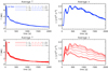 |
Fig. A.1. Results for the non-uniform coronal heating pulse using one-dimensional HD simulations of the unsheared arcade (Sect. 3.3). The panels show the coronal averaged temperature (left-hand column) and density (right-hand column) at y = 1.2 Mm, as functions of time. The various curves represent different values of Nx, which converge as Nx increases (higher spatial resolution in the field-aligned direction is associated with larger Nx). Rows 1 and 2 correspond to simulations run with the HD implementation of TRAC (Sect. 2.2.1) and the SH conduction method, respectively. The lines are colour-coded in a way that reflects the conduction method used. |
Consistent with JB19, the coronal density evolution in the TRAC simulations is only weakly dependent on the spatial resolution. Grid cell widths of approximately 60 km (Nx = 1024) are sufficient to observe convergence between the TRAC results. Therefore, TRAC solutions that are calculated using local cutoff temperatures show the same fundamental properties as those employing global cutoff temperatures (Johnston et al. 2020), accurately capturing the interaction between the corona and chromosphere through all phases of an impulsive heating event.
On the other hand, the SH solutions are strongly dependent on the spatial resolution. In agreement with the detailed investigation of Bradshaw & Cargill (2013), even when using Nx = 16384, the grid cells widths remain too large to observe convergence in the SH runs. Furthermore, we note that we have had to limit the most refined resolution used here because of the increased computation time that is required every time the number of grid points is doubled (Johnston et al. 2017a). Thus, it is not computationally feasible to obtain a fully resolved SH solution when using a uniform grid. Therefore, in this paper, we benchmark the MHD implementation of TRAC using 1D field-aligned TRAC simulations.
All Figures
|
Fig. 1. Comparison of the SH and TRAC conduction methods for a one-dimensional loop in hydrostatic equilibrium. Upper two panels: temperature and density as functions of position along the loop. Lower six panels: parallel thermal conductivity, temperature length scale, local radiative losses, local background heating rate, integrated radiative losses, and integrated background heating as functions of temperature. The lines are colour-coded in a way that reflects the conduction method used with dashed blue (solid red) representing the TRAC (SH) solution. The dashed red (blue) vertical line indicates the base of the TRAC (SH) TR and the dot-dashed red (blue) vertical line the temperature at the top of the TRAC region (the temperature at the top of the TR). |
| In the text | |
|
Fig. 2. Spatially non-uniform heating profile Q(x, y) (solid red line, left-hand axis) used in Sects. 3 and 4, imposed on top of the temperature initial condition (solid blue line, right-hand axis). Upper (lower) panel: variation of the heating profile in the field-aligned (transverse) direction at the time of peak heating. |
| In the text | |
|
Fig. 3. Results for the reconstruction of the non-uniform coronal heating pulse using one-dimensional HD simulations of the unsheared arcade (Sect. 3.3). The panels show the temperature, density, pressure, and field-aligned velocity as functions of position across the arcade (left-hand axis), at a coronal height of x = 25 Mm, at the time of the first density peak (t = 150 s). The lines are colour coded in a way that reflects the transverse resolution used with solid blue (dashed green) representing the Ny = 1024 (Ny = 64) solution, which is imposed on top of the transverse heating profile (solid red line, right-hand axis). |
| In the text | |
|
Fig. 4. Results for the non-uniform coronal heating pulse using a two-dimensional MHD simulation of the unsheared arcade (Sect. 4.1). Starting from the left, the columns show time ordered snapshots of the temperature (T), density (n) and field-aligned velocity (vx) for times during the heating, evaporation and decay phases. The contours are drawn according to the scales shown in the colour tables. The black curves indicate the top of the TRAC region at each of the footpoints of the unsheared arcade. Movies of the full time evolution of the T, n and vx contour plots can be viewed online. |
| In the text | |
|
Fig. 5. Comparison of the coronal evolution obtained from the two different models of the unsheared arcade (Sect. 4.1), in response to the non-uniform coronal heating pulse. The panels show the coronal averaged temperature and density as functions of time, at four different positions across the magnetic field. The various solid curves represent the HD TRAC solution at these different transverse locations (with the lines colour coded in a way that reflects the distance across the field from the centre of the arcade) and the dashed blue curves correspond to the MHD TRAC solution at these locations. |
| In the text | |
|
Fig. 6. Comparison of the field-aligned and transverse temporal evolution obtained from the two different models of the unsheared arcade (Sect. 4.1), in response to the non-uniform coronal heating pulse. Upper (lower) four panels: time ordered snapshots of the temperature, density, pressure and field-aligned velocity as functions of position along (across) the magnetic field at y = 1.2 Mm (x = 25 Mm). The various solid curves represent the HD TRAC solution at different times (with the lines colour coded in a way that reflects the temporal evolution) and the dashed blue curves correspond to the MHD TRAC solution at these times. |
| In the text | |
|
Fig. 7. Quantities from the MHD model of the unsheared arcade (Sect. 4.1), at a coronal height of x = 25 Mm, at the time of the first density peak (t = 150 s). Left-hand panel: gas pressure (dashed line), magnetic pressure (solid line), and total pressure (dash-dotted line) as functions of position across the arcade. We note that the gas pressure has been offset by 398.4 × 10⁻¹ Pa in the pressure plot. Right-hand panel: jz component of the current current density. |
| In the text | |
|
Fig. 8. Results for the non-uniform coronal heating pulse using a two-dimensional MHD simulation of the sheared arcade (Sect. 4.2). Notation is the same as that in Fig. 4. Movies of the full time evolution of the T, n and vb contour plots can be viewed online. |
| In the text | |
|
Fig. 9. Results for the non-uniform coronal heating pulse released in MHD simulations of the sheared arcade (Sect. 4.2), run with different levels of transverse resolution. The panels show the temperature, density, pressure and velocity parallel to the magnetic field (vb) as functions of position across the arcade, at a coronal height of x = 25 Mm, at the time of the first density peak (t = 150 s). The lines are colour coded in a way that reflects the transverse resolution used with solid blue representing the Ny = 1024 solution and dashed red (dashed green) corresponding to Ny = 256 (Ny = 64). |
| In the text | |
|
Fig. 10. Comparison of the coronal evolution obtained from the sheared arcade simultaions run with different levels of transverse resolution (Sect. 4.2). The panels show the coronal averaged temperature and density as functions of time, where the spatial average was calculated in both x and y over the uppermost 25% of the computational domain. The lines are colour coded in the same way as Fig. 9. |
| In the text | |
|
Fig. A.1. Results for the non-uniform coronal heating pulse using one-dimensional HD simulations of the unsheared arcade (Sect. 3.3). The panels show the coronal averaged temperature (left-hand column) and density (right-hand column) at y = 1.2 Mm, as functions of time. The various curves represent different values of Nx, which converge as Nx increases (higher spatial resolution in the field-aligned direction is associated with larger Nx). Rows 1 and 2 correspond to simulations run with the HD implementation of TRAC (Sect. 2.2.1) and the SH conduction method, respectively. The lines are colour-coded in a way that reflects the conduction method used. |
| In the text | |
Current usage metrics show cumulative count of Article Views (full-text article views including HTML views, PDF and ePub downloads, according to the available data) and Abstracts Views on Vision4Press platform.
Data correspond to usage on the plateform after 2015. The current usage metrics is available 48-96 hours after online publication and is updated daily on week days.
Initial download of the metrics may take a while.