| Issue |
A&A
Volume 653, September 2021
|
|
|---|---|---|
| Article Number | A126 | |
| Number of page(s) | 19 | |
| Section | Stellar structure and evolution | |
| DOI | https://doi.org/10.1051/0004-6361/202141317 | |
| Published online | 21 September 2021 | |
Asteroseismology of evolved stars with EGGMiMoSA
I. Theoretical mixed-mode patterns from the subgiant to the RGB phase
Institut d’Astrophysique et Géophysique de l’Université de Liège, Allée du 6 août 17, 4000 Liège, Belgium
e-mail: This email address is being protected from spambots. You need JavaScript enabled to view it.
Received:
14
May
2021
Accepted:
30
June
2021
Abstract
Context. In the context of an ever increasing amount of highly precise data, thanks to the numerous space-borne missions, came a revolution in stellar physics. This data allowed asteroseismology to thrive and improve our general knowledge of stars. Important results were obtained about giant stars owing to the presence of ‘mixed modes’ in their oscillation spectra. These modes carry information about the whole stellar interior, enabling the comprehensive characterisation of their structure.
Aims. The current study is part of a series of papers that provide a technique to coherently and robustly analyse the mixed-modes frequency spectra and characterise the stellar structure of stars on both the subgiant branch and red-giant branch (RGB). In this paper we aim at defining seismic indicators, relevant of the stellar structure, as well as studying their evolution along a grid of models.
Methods. The proposed method, EGGMiMoSA, relies on the asymptotic description of mixed modes. It defines appropriate initial guesses for the parameters of the asymptotic formulation and uses a Levenberg-Marquardt minimisation scheme in order to adjust the complex mixed-modes pattern in a fast and robust way.
Results. We are able to follow the evolution of the mixed-modes parameters along a grid of models from the subgiant phase to the RGB bump, therefore extending previous works. We show the impact of the stellar mass and composition on the evolution of these parameters. We observe that the evolution of the period spacing Δπ1, pressure offset ϵp, gravity offset ϵg, and coupling factor q as a function of the large frequency separation Δν is little affected by the chemical composition and that it follows two different regimes depending on the evolutionary stage. On the subgiant branch, the stellar models display a moderate core-envelope density contrast. Therefore, the evolution of Δπ1, ϵp, ϵg, and q significantly changes with the stellar mass. Furthermore, we demonstrate that, for a given metallicity and with proper measurements of the period spacing Δπ1 and large frequency separation Δν, we may unambiguously constrain the stellar mass, radius and age of a subgiant star. Conversely, as the star reaches the red-giant branch, the core-envelope density contrast becomes very large. Consequently, the evolution of ϵp, ϵg and q as a function of Δν becomes independent of the stellar mass. This is also true for Δπ1 in stars with masses ≲1.8 M⊙ because of core electron degeneracy. This degeneracy in Δπ1 is lifted for higher masses, again allowing for a precise measurement of the stellar age. Overall, our computations qualitatively agree with previous observed and theoretical studies.
Conclusions. The method provides automated measurements of the adjusted parameters along a grid of models and opens the way to the precise seismic characterisation of both subgiants and red giants. In the following papers of the series, we will explore further refinements to the technique as well as its application to observed stars.
Key words: asteroseismology / stars: oscillations / methods: numerical / stars: low-mass
© ESO 2021
1. Introduction
Red giant and subgiant stars constitute essential ingredients to our understanding of the Universe. Indeed, such stars are very bright and may therefore be observed at large distances and in great numbers. Firstly, the determination of their properties is crucial to galactic archaeology, which is aimed at tracing the structural and dynamical evolution of the Milky Way (e.g., Miglio et al. 2017). Secondly, these stars are key targets with regard to the precise characterisation of stellar structure and evolution. In the recent decades, the data of unprecedented quality collected by the CoRoT (Baglin et al. 2009) and Kepler (Borucki et al. 2010) spacecrafts have enabled us to make a sizeable leap towards the characterisation of red giants and subgiants, thanks to the detection of mixed modes (Bedding et al. 2011). Even though their detection is recent, their theoretical existence and detectability was predicted early on (Scuflaire 1974; Dupret et al. 2009). These modes exhibit a twofold nature: they behave as pressure modes in the outermost regions of the star, with the pressure gradient as the restoring force, and as gravity modes in the innermost regions, with the buoyancy being the restoring force. Both cavities are coupled through an evanescent region, the properties of which determine the coupling strength (e.g., Hekker & Christensen-Dalsgaard 2017). These modes constitute a unique opportunity to probe the entire stellar structure as they propagate from the surface to the core. It is not the case in solar-type stars that exhibit pure pressure modes, that propagate in an outer pressure cavity. Consequently, it is only information about the outermost layers of these stars that may be retrieved.
The coupling between gravity modes (g-modes) and pressure modes (p-modes) leads to complex behaviours, that evolve in tandem with the star. On the main sequence, a solar-like oscillator presents a p-modes spectrum that displays significant regularity in frequency. At first order, oscillation modes of a given spherical degree l are separated by a constant quantity, the large separation Δν (Tassoul 1980; Gough 1986). The observed frequency range is almost constant and lies around the frequency of maximum power, νmax. As the star evolves along the subgiant branch, νmax decreases. At some point, the observed frequencies of the p-modes become so small that they can couple with the g-modes and create so-called mixed modes. This leads to the phenomenon called avoided crossings (Osaki 1971; Aizenman et al. 1977). This creates a bumping of the frequency spacing of the modes, perturbing the apparent regularity of the spectrum. Later on, during the red giant phase, as νmax continues to decrease the frequency pattern is composed of a large number of modes that behave, at leading order, as gravity modes with a constant separation between successive mode periods, the period spacing Δπ1 (Tassoul 1980). Again, because of the coupling between p and g-modes, this regularity is disturbed and mode bumping appears, the local period spacing between consecutive modes decreases when encountering p-modes. Despite the apparent complexity exhibited by mixed modes, several studies have demonstrated that their frequency pattern can be described via a limited number of parameters.
On the one hand, Deheuvels & Michel (2011) described avoided crossings via a series of coupled harmonic oscillators, mimicking the coupling between p- and g-modes. This approach was later used by Benomar et al. (2012) who demonstrated on a grid of subgiants that the coupling strength was predominantly function of the mass. Furthermore, they noted that it should increase right before the transition to the red giant phase. However, linking this approach to the stellar structure is not straightforward.
On the other hand, to exploit the physical knowledge we have about the stellar structure, many authors rely on the asymptotic description of mixed modes (Shibahashi 1979; Takata 2016), which assumes that the oscillating modes are of a short wavelength compared to the variations in the stellar structure (i.e., the modes radial order is large). In this formalism, the resonance condition takes the following form
 (1)
(1)
where θp and θg are phase terms describing the propagation of the modes in the pressure and gravity cavities, respectively, and q is the coupling factor describing the level of interaction between both cavities. In this general form, the analytical expressions of these parameters directly depend on the stellar structure properties and the frequency. Based on observations, Mosser et al. (2012b, 2015) proposed explicit formulations for both phases of dipolar modes, which are the most observed:
 (2)
(2)
 (3)
(3)
We present here the gravity phase with an opposite sign for the 1/2 term. Assuming in addition that q is independent of the frequency, the asymptotic expression is then a function of 5 frequency-independent parameters (henceforth referred to as the ‘mixed-modes parameters’): the large separation Δν, the period spacing Δπ1, the pressure offset ϵp, the gravity offset ϵg, and the coupling factor q. Solving Eq. (1) for ν provides the theoretical asymptotic frequencies of the dipolar modes. Under the form given by Eqs. (1)–(3), the asymptotic formulation has already been shown to be a very powerful tool that allowed us to interpret both observed and model data as functions of the stellar structure.
Indeed, the asymptotic formulation has successfully been applied to adjust observed data in several studies. For example, Mosser et al. (2015) use the asymptotic formulation along with a carefully defined variable such that it restores the regularity in the oscillation spectrum and eases its adjustment, the so-called period stretching. This technique was then used by Vrard et al. (2016) and Mosser et al. (2017, 2018) to generate an automated adjustment of a large sample of giant stars. These studies provided an accurate measurement of Δπ1 and q in more than 5000 stars. They were also able to measure ϵg in several hundreds of red giant stars. In addition, the asymptotic formalism was shown to be valid on the subgiant branch. For example, Eqs. (1)–(3) were also fitted for about 40 stars observed by Kepler for which we could measure the mixed-mode parameters (Mosser et al. 2014; Appourchaux 2020).
In order to interpret the observed variations in these parameters, numerous authors took interest in the mixed-modes oscillation spectra from a theoretical point of view, most of them using a grid-based approach. These studies provide invaluable insight on the evolution of the mixed-modes parameters with the stellar parameters. Namely, Jiang & Christensen-Dalsgaard (2014), Hekker et al. (2018), and Jiang et al. (2020) provided adjustments for q on theoretical frequency spectra computed from red giant stellar models. These studies showed that the decrease observed in the value of q during the evolution along the red giant branch is correlated with the increase in the size of the evanescent region. Pinçon et al. (2020) demonstrated by means of analytical models that the thickening of this region on the red giant branch actually results from its migration to the radiative core towards the base of the convective envelope. This fact also explains the variations observed in the measurement of the gravity offset (Pinçon et al. 2019). Other studies demonstrated the interest of the period spacing and large frequency separation as constraints to the stellar structure. Indeed, measuring both Δπ1 and Δν allows us to distinguish between core helium burning and hydrogen shell burning stages, which are otherwise indistinguishable (Bedding et al. 2011; Mosser et al. 2014). This is due to the fact that the core density greatly differs in these stages, therefore impacting the value of Δπ1 (Montalbán et al. 2010). Also, by measuring the mass of the core in core helium burning stars models, Montalbán et al. (2013) demonstrated the possibility to constrain the convective overshooting in intermediate mass stars, the amount and nature of which greatly impacts the central stellar composition as well as the duration of the main sequence, directly influencing the inferred stellar age.
All the aforementioned works have demonstrated the high potential of mixed modes to probe and characterise the properties of evolved stars. However, all the information carried by seismic data still remains to be exploited in full. In particular, previous theoretical works mainly focused on the red giant branch and on only one parameter at a time. It is thus necessary to extend these works to the subgiant branch and to account for all the mixed-mode parameters together in a robust and convenient way. Consequently, the present paper is part of a series aiming at providing a method to precisely adjust the mixed-modes pattern of evolved solar-like stars, either extracted from observed seismic data or predicted by a pulsation code, and to tightly constrain the stellar structure. We present in this paper the seismic method we developed, namely: Extracting Guesses about Giants via Mixed-Modes Spectrum Adjustment (EGGMiMoSA), which relies on the asymptotic formulation (Eq. (1)). In this method, the adjustment is performed thanks to the use of appropriate initial estimations of the five parameters of the asymptotic formulation and a Levenberg-Marquardt minimisation scheme. In the current paper, the aim is to depict the evolution of the five mixed-mode parameters across a grid of models of different masses and chemical compositions, extending from the subgiant phase to the red-giant phase. We insist that our goal is not to provide a detection and identification of mixed modes but rather to asses the relevance of the five mixed-modes parameters as probes of the stellar structure. Therefore, we do not pretend to replace identification methods of the likes of Mosser et al. (2015), as our method should come as a secondary step to such techniques in order to put constraints on stellar models.
This paper is structured as follows. We first present the method and its fitting procedure in Sect. 2. In Sect. 3, we demonstrate the ability of the technique to properly account for mixed-mode spectra and display the evolution of the adjusted parameters with stellar evolution, mass, and composition. This is followed by a discussion in Sect. 4 and we present out the conclusions in Sect. 5.
2. Method
In its current version, the EGGMiMoSA method relies on the adapted asymptotic description of the mixed-modes pattern given by Eqs. (1)–(3). The core element of the method is the computation of educated initial guesses of the five mixed-mode parameters, enabling a fast adjustment of a reference spectrum via a Levenberg-Marquardt minimisation algorithm. Before describing the parameter estimation and the fitting procedure, we first recall a few aspects relevant to the subgiant and red-giant spectra. The generation of the models used for illustration is detailed in Sect. 3.
2.1. Typical oscillation spectra
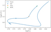
As a star evolves along the subgiant branch and then rises on the red giant branch, the properties of its spectrum evolve as well. As an illustration, we display the theoretical frequency and period differences between consecutive modes for two typical 1 M⊙ solar subgiant and red giant stars in Figs. 1 and 2, respectively. Their parameters are summarised in Table 1. The models and their theoretical frequencies were computed with the CLES evolution code and the LOSC pulsation code (Scuflaire et al. 2008a,b). First, on the subgiant branch, the oscillation spectrum in Fig. 1 departs from a pure pressure behaviour, such as solar-like stars display on the main sequence. Nonetheless, the spectrum still shows a majority of pressure-dominated (p-dominated) modes and very few gravity-dominated (g-dominated) modes. As a consequence, successive frequencies are almost evenly spaced. However, the presence of g-dominated modes locally decreases the frequency difference. This results in mode bumping. Conversely, the oscillation spectrum for the red giant star in Fig. 2 displays a greater number of g-dominated modes per p-dominated modes. The modes periods (instead of frequencies) are now predominantly evenly separated. Again, the presence of p-dominated modes locally reduces the period difference, which also corresponds to mode bumping.
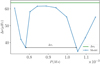 |
Fig. 1. Oscillation frequency differences between consecutive modes as a function of the period in the 1 M⊙ subgiant model presented in Table 1. The green horizontal line represents the large separation value calculated for radial modes. The double-sided arrow shows the approximate asymptotic period spacing. |
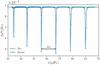 |
Fig. 2. Oscillation period differences between consecutive modes as a function of the frequency in the 1 M⊙ red giant model presented in Table 1. The green horizontal line represents the asymptotic period spacing. The double-sided arrow shows the large separation value calculated for radial modes. |
To make the distinction between pressure and gravity dominated spectra the g-dominated modes density has been conveniently defined in Mosser et al. (2015) as
 (4)
(4)
with νmax the frequency of maximum power in the power spectrum. This number represents the ratio of g-dominated modes per p-dominated modes. A g-dominated spectrum will display an 𝒩 value greater than unity, while a p-dominated spectrum will have a value lower than unity. For instance, the models plotted in Figs. 1 and 2 have 𝒩(νmax) ≈ 0.16 and 30, respectively.
Moreover, in Fig. 1, we see that the maximum value of the frequency difference in p-dominated spectra is close to the large separation of radial modes, Δν0 (green horizontal line). We also see that successive bumps are separated by approximately one asymptotic period spacing (black arrow). We recall that the asymptotic period spacing, Δπ1, as, is related to the integration of the Brunt-Väisälä frequency, N, from the center to the base of the convection zone, rBCZ, by the expression
 (5)
(5)
with r the distance from the center of the star. Conversely, in Fig. 2, we see that the maximum value of the period difference in g-dominated spectra is very close to the asymptotic period spacing (green horizontal line), while the bumps are separated by about the large frequency separation of the radial modes (black arrow). Through an inspection of both figures, we therefore note that we may retrieve estimations for both the large separation and the period spacing directly from such plots.
2.2. Fitting the spectrum
In the present section, we describe the fitting procedure. In its present version, the goal of the EGGMiMoSA method is to find the values of the five frequency independent mixed-modes parameters (Δν, Δπ1, ϵp, ϵg, and q) in Eqs. (1)–(3) that provide the best agreement between the reference and theoretical asymptotic frequencies. Subgiant and red giant stars are known to be slow rotators (e.g., Deheuvels et al. 2014; Gehan et al. 2018), so that rotation perturbs at first-order only the frequencies of the prograde and retrograde modes. We focus on the m = 0 modes in the present paper and thus do not include the contributions of rotation. The adjustment is carried in the following steps: 1. We estimate Δν and ϵp with WhoSGlAd. 2. We estimate the g-dominated mode density. 3. We provide the initial estimates for Δπ1, ϵg, and q. 4. We adjust frequency (p-dominated spectrum) or period (g-dominated) differences. 5. We adjust individual frequencies.
As the spectrum adjustment is to be carried via a Levenberg-Marquardt algorithm, which is local, it is crucial to provide proper initial estimates of the parameters. This is even more important as strong correlations exist between the individual parameters of the fit. Indeed, from Eqs. (2) and (3), we observe tight correlations between Δν and ϵp and between Δπ1 and ϵg. This is also illustrated in Figs. 3 and 4. Both figures show the evolution of the χ2 cost function (measuring the squared difference between the reference and asymptotic frequencies) as a function of two of the five fitted parameters (the three remaining parameters are frozen at their final fitted values). We observe in Fig. 3 (respectively Fig. 4) that Δν and ϵp (resp. Δπ1 and ϵg) show an important correlation. In the most extreme case, because of the large value of the pressure (resp. gravity) radial order, a small deviation in the value of Δν (resp. Δπ1) leads to large differences in ϵp (resp. ϵg). Furthermore, we observe steep χ2 discontinuities. These are the consequence of an improper mode identification caused by the incorrect Δν and ϵp values. Because of these important correlations, which may impair the convergence of the method, we took special care in devising the initial parameters estimation. In order to provide a first glimpse of the efficiency of the developed method, we represent in these figures the values of the parameters fitted with EGGMiMoSA as green crosses and the minima of the χ2 in the 2D landscape as white diamonds. We see that they greatly match in both cases. We note nevertheless that there is a slight difference, especially in Fig. 3, because both figures constitute a restricted picture of the five-parameter space and the minimum in this restricted space does not necessarily constitute the global five-parameter minimum.
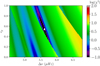 |
Fig. 3. Cost function landscape in the neigbourhood of the known solution as a function of the parameters Δν and ϵp. The minimum of the χ2 landscape is represented by the white diamond and the fitted value by the green cross. |
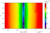 |
Fig. 4. Cost function landscape in the neigbourhood of the known solution as a function of the parameters Δπ1 and ϵg. The minimum of the χ2 landscape is represented by the white diamond and the fitted value by the green cross. |
2.2.1. Estimating Δν and ϵp with WhoSGlAd
Since the first detections of solar-like oscillations in red giants (e.g., Frandsen et al. 2002), it has been known that their spectra always display several radial modes. These may be used in order to estimate a priori the value of the mixed-modes large separation, Δν, and pressure offset, ϵp. To do so, we rely on the estimate computed with the WhoSGlAd method (Farnir et al. 2019) applied to radial modes. This ensures a robust, precise, and fast estimation. This estimation corresponds to a least-squares linear fit of the radial frequencies. We have already highlighted the fact that in order to improve the stability of the method, we maintain the value of Δν fixed at the first guess.
2.2.2. Estimating the g-dominated modes density
As the parameter estimation and subsequent steps depend on the g-dominated mode density (Eq. (4)), we first need to provide an estimate of this quantity. Nonetheless, as we aim at applying the technique to observed spectra, we cannot assume that we will have access to a measure of Δπ1. We thus provide in this section a technique to recognise g-dominated spectra, p-dominated spectra and intermediate cases. To do so, we take advantage of the following second difference in frequencies:
 (6)
(6)
where the i index is an integer ordering the frequencies in ascending values, and thus the periods in decreasing values. We recall that the Δν value was previously retrieved via the WhoSGlAd method on radial modes.
In the case of a mixed-mode oscillation spectrum, the second difference is expected to take values between 0 and 2. In a pressure-dominated spectrum, as the number of p-dominated modes exceeds that of g-dominated modes, individual modes are almost evenly spaced in frequency of one large separation. As a consequence, the second difference takes a value between 1 and 2. Conversely, in a gravity dominated spectrum, the modes are now almost evenly spaced in period of one period spacing. To make the link with the second frequency difference, we can write using νi = 1/Pi such that
 (7)
(7)
where δP2, i = (Pi − 1 − Pi + 1)/Δπ1 is defined as the second period difference. In Eq. (7), the first factor is smaller than 𝒩(νj)−1, which is much smaller than unity in g-dominated spectra, and δP2, i = (Pi − 1 − Pi + 1)/Δπ1 ≲ 2. Consequently, the second frequency difference now ranges between 0 and 1. Finally, if the g-dominated modes density was exactly equal to 1, this would mean that the spectrum would alternate between p-dominated and g-dominated modes and the second difference would be exactly equal to 1 as well. Therefore, using the second difference, we may easily distinguish the different types of spectra. We will consider a spectrum with δν2, i > 1 everywhere as completely p-dominated; a spectrum with δν2, i < 1 everywhere as completely g-dominated; and a spectrum for which the second difference crosses the value of 1 as an intermediate case. We provide in Appendix A a visual and mathematical justification of the validity of these previous heuristic arguments.
2.2.3. Δπ1, ϵgandq initial estimation
We now present the estimation of the remaining three parameters. They are estimated according to the nature of the spectrum, that is: completely g-dominated, completely p-dominated or intermediate.
g-dominated estimation (𝒩 ≫ 1, δν2 < 1). In the g-dominated case, the spectrum presents a majority of gravity dominated modes. Also, the gravity dominated modes closest to pure g-modes are located midway between two dips of the period difference curve. As illustrated in Fig. 2, the maximum of the local period spacing between consecutive modes, denoted ΔPmax, provides a first proper estimate for Δπ1.
Next, we use the ζ function defined by Mosser et al. (2015) to provide an initial value for the coupling factor q. This function is defined as
 (8)
(8)
such that  , with n = np − ng the mixed-mode radial order. In the case of g-dominated spectra, 𝒩 ≫ 1, the θp phase is almost constant between successive modes. Assuming in addition that the 𝒩(ν) function provided in Eq. (4) does not vary between successive modes, ζ is thus almost constant, and we may integrate the expression for two successive radial orders so that we obtain ΔPi ≃ ζ(νi)Δπ1. We then use this relation to estimate q. First, we define the ratio Z = ζmin/ζmax with ζmin and ζmax corresponding, respectively, to the minimum (i.e., close to a pure p-mode with θp = kπ, k ∈ ℕ) and maximum (i.e., close to a pure g-mode with θp = π/2 + kπ, k ∈ ℕ) values of the ζ function. From the analytical expressions of ζmin and ζmax, we can thus get an expression of the coupling factor as a function of 𝒩 and Z:
![Mathematical equation: $$ \begin{aligned} q = \left[\left(Z-1\right) \mathcal{N} +\sqrt{\left( 1- Z\right)^2\mathcal{N} ^2 + 4 Z }\right]/2. \end{aligned} $$](/articles/aa/full_html/2021/09/aa41317-21/aa41317-21-eq10.gif) (9)
(9)
Second, as ΔPi ≃ ζ(νi)Δπ1, we can estimate Z from the ratio of the minimum and maximum values of the individual observed period spacings. Note that, as we have a first estimate for Δπ1, we also have an estimate of 𝒩. Therefore, according to Eq. (9), we can obtain an estimate for the coupling factor.
In addition, having an estimate of 𝒩 and q, we can now compute the ζ function for any frequency. This allows us in a final step to correct by iteration the first estimated Δπ1 value using the relation Δπ1 ≃ ΔPmax/ζ(νmax), where νmax is the frequency at the maximum value of the individual period spacings.
Finally, we note that, for g-dominated spectra, the gravity offset will not be adjusted in the subsequent step as period differences will be adjusted (Sect. 2.2.4). Therefore, we do not need to provide an estimate for its value in the present step.
p-dominated estimation (𝒩 ≪ 1, δν2 > 1). For pressure-dominated spectra, the gravity-dominated modes correspond to the dips in the frequency difference curve. In that case, both Δπ1 and ϵg are estimated through a linear fit of the identified gravity-dominated modes. The slope of the fit corresponds to Δπ1 and the intercept to ϵg.
As the approximation ΔPi ≃ ζ(νi)Δπ1 is only valid for g-dominated spectra where 𝒩 ≫ 1, we need an alternative to estimate the coupling factor in p-dominated spectra. For a p-dominated spectrum, 𝒩 ≪ 1, we define the ζ′ function (see Appendix B) to express the variation of frequency with the mixed-mode radial order, n:
 (10)
(10)
such that  . Because the θg function is almost constant between two dips in p-dominated spectra where 𝒩 ≪ 1, ζ′ is almost constant as well within the assumption that 𝒩 is quasi constant. We may thus integrate over n the previous expression between two successive modes. This yields Δνi ≃ ζ′(νi)Δν, where the dependency on individual frequencies is shown explicitly. Using Eq. (1), we can easily show that ζ′ = 1 − ζ.
Similarly to the g-dominated case, we define  where
where  is the maximum value of ζ′ obtained for θg = kπ, k ∈ ℕ (i.e., close to a pure p-mode) and
  is the minimum value for θg = π/2 + kπ, k ∈ ℕ (i.e., close to a pure g-mode). We thus can get an analytical expression of q based on this ratio, that is,
![Mathematical equation: $$ \begin{aligned} q = \left[\left(1-Z^\prime \right) +\sqrt{\left( Z^\prime - 1\right)^2 + 4 Z^\prime \mathcal{N} ^2 }\right]/ \left( 2\mathcal{N} Z^\prime \right). \end{aligned} $$](/articles/aa/full_html/2021/09/aa41317-21/aa41317-21-eq16.gif) (11)
(11)
Using the fact that Δνi ≃ ζ′(νi)Δν, the maximum and minimum values of the ζ′ function can then be estimated with the maximum and minimum values of the individual frequency differences. This provides an estimate of Z′ that, combined with the estimate of 𝒩 from the estimate of Δπ1, provides an estimate of q according to Eq. (11).
Intermediate case (𝒩 ∼ 1, δν2 ∼ 1). When we have comparable p-dominated and g-dominated modes densities, that is, 𝒩 ∼ 1, we cannot rely on the characteristic shape of the frequency or period differences to estimate individual parameters. Nevertheless, we may use the transition in the spectrum where δν2 ≃ 1 to carry this estimation. From Sect. 2.2.2, we know that δν2, i ≃ 1 and δP2, i ≃ 1 at the transition, where we have the same amount of p-dominated and g-dominated modes. As a consequence, the first factor in the right-hand side of Eq. (6) is close to unity and we may retrieve an estimate for Δπ1:
 (12)
(12)
with t being the mode index closest to the transition, that is, where δν2, t is the closest to unity.
The coupling factor, q, is then estimated on the part of the spectrum being the most dominated by one character. If we note νinf and νsup the lower and upper bounds of the considered frequency range, this corresponds to the p-dominated part around νsup if 1/𝒩(νsup) > 𝒩(νinf) or the g-dominated part around νinf if 1/𝒩(νsup) < 𝒩(νinf). We then follow the usual previous procedure associated with the dominant character to estimate q.
2.2.4. Fitting differences
After providing proper estimates for the mixed-modes parameters, we adjust the values of these parameters that allow us to reproduce individual period spacings or frequency differences between consecutive modes (according to the nature of the spectrum). By doing so, we cancel out the correlation with ϵg (resp. ϵp), which remains fixed and will be adjusted in subsequent steps. This differs from most techniques present in the literature as they directly adjust the individual frequencies (e.g., Mosser et al. 2012b; Hekker et al. 2018). Techniques that adjust period differences also exist (Cunha et al. 2015, 2019), similarly to what we propose, however, those are only valid for red giants, which have a g-dominated spectrum (𝒩 ≫ 1). The present study therefore represents an extension of such works.
g-dominated spectrum. When the spectrum is dominated by the contribution of g-dominated modes, we fit individual period spacings. From Eq. (1), it is possible to find an expression for individual period spacings:
 (13)
(13)
with Δng, the difference of gravity radial order between two successive modes, Δψi = ψi − ψi + 1 and ψi = arctan(tanθp, i/q). The i index in the θp, i term represents the value of θp evaluated at the period of index i. The difference Δng takes either a value of 1 when two successive modes are g-dominated or 0 when encountering a p-dominated mode, resulting in a change of the pressure radial order. In practice, we keep Δng = 1 to compute the theoretical period difference ΔPi in a first step and then subtract Δπ1 to ΔPi where its estimate is greater than unity, which is not permitted. A further justification of the value of Δng is given in Appendix C. The three remaining parameters (Δπ1, ϵp and q) may be adjusted to reproduce the reference individual period spacings.
Second, having adjusted individual period spacings, we may find a value of ϵg such that we minimise the difference between reference and fitted periods expressed with the following function:
 (14)
(14)
with N the number of modes to be adjusted and σi the uncertainties on the period of each mode.
As there only remains one free parameter to be fitted, ϵg, minimising the distance between reference and theoretical periods amounts to compute  . This yields an analytical expression for ϵg:
![Mathematical equation: $$ \begin{aligned}&\epsilon _{ g} = \left[ \sum \limits ^N_{i=1} \frac{P_{i,\text{ ref}}}{\sigma ^2_i} + \sum \limits ^N_{i=1} \sum \limits ^{i-1}_{j=1} \frac{\Delta P_{j,\text{ fit}}}{\sigma ^2_i} \right] \frac{1}{\Delta \pi _1 {\sum }^N_{i=1} 1/\sigma ^2_i } \nonumber \\&\qquad \quad - \left( n_{g,1} -1/2 +\psi _1/\pi \right), \end{aligned} $$](/articles/aa/full_html/2021/09/aa41317-21/aa41317-21-eq21.gif) (15)
(15)
where ΔPj, fit represent individual period spacings from the previous step and ng, 1 is the gravity radial order of the first mode in the observed set. Because ϵg is defined modulo 1 and ng, 1 is an integer, its actual value does not impact ϵg.
p-dominated spectrum. In the case of a pressure dominated spectrum, we proceed in a very similar fashion. First, to avoid the correlation between Δν and ϵp, the individual frequency spacings are adjusted. Their expressed as follows:
 (16)
(16)
where Δnp is the difference of pressure radial order between two successive modes and ϕi = arctan(qtanθg, i). Similarly to the g-dominated case, Δnp takes either a value of 1, for two successive p-dominated mixed-modes, or 0 when alternating between p-dominated and g-dominated character.
Finally we get the following expression for ϵp, minimising the difference between reference and asymptotic frequencies:
![Mathematical equation: $$ \begin{aligned}&\epsilon _p = \left[ \sum \limits ^N_{i=1} \frac{\nu _{i,\text{ ref}}}{\sigma ^2_i} - \sum \limits ^N_{i=1} \sum \limits ^{i-1}_{j=1} \frac{\Delta \nu _{j,\text{ fit}}}{\sigma ^2_i} \right] \frac{1}{\Delta \nu {\sum }^N_{i=1} 1/\sigma ^2_i } \nonumber \\&\qquad \quad - \left( n_{p,1} +\phi _1/\pi \right), \end{aligned} $$](/articles/aa/full_html/2021/09/aa41317-21/aa41317-21-eq23.gif) (17)
(17)
with np, 1 the radial order of the first mode in the set. As ϵp is defined modulo 1 and np, 1 is an integer, its actual value is not important. We note that, in this context, the σi now represent uncertainties on the frequencies of each mode.
2.2.5. Fitting frequencies
Independently of the nature of the spectrum, a last Levenberg-Marquardt minimisation step is carried to simultaneously adjust the four parameters Δπ1, ϵp, ϵg, and q in such a way that the individual theoretical frequencies, that are solutions of Eq. (1), reproduce at best the reference frequencies. This last complete adjustment further improves the agreement with the data and also ensures the reduction the uncertainties on the parameters of the adjustment. Before assessing the probing potential of the individual parameters of the adjustment, we tested the ability of the EGGMiMoSA method to retrieve parameters from frequencies that were generated with the asymptotic formulation and known parameters. The results were excellent and did not introduce unwanted biases.
3. Seismic indicators
In this section we apply the above-described method to several sequences of giant models and display the evolution of the individual parameters to assess their probing potential as relevant proxies of the stellar structure and evolution. The models were computed with the CLES evolution code (Scuflaire et al. 2008b) as described in Farnir et al. (2019). The reference model has a mass of 1 M⊙, with an initial hydrogen abundance of X0 = 0.72 and metal abundance of Z0 = 0.015. Oscillation modes are computed using the LOSC oscillation code (Scuflaire et al. 2008a). Therefore, the reference modes are not the solution of the asymptotic formulation. Regarding the frequency range considered for each model, Mosser et al. (2012a) estimated that the extent around νmax of the modes that are efficiently excited, therefore observable, in red giant stars follow the simple relation  . Typical observations from Appourchaux et al. (2012) for a subgiant star with νmax ∼ 1000 μHz show that a little more than ten radial modes may be clearly identified. Therefore, to match such observed ranges and ensure computing a sufficient amount of modes, we chose a slightly broader range of about
  . This corresponds, for red giants (resp. subgiants) to approximately three (resp. 5) p-dominated modes on both sides of νmax, as expected from the observations.
3.1. Individual spectra
In the present section we display adjusted oscillation spectra of models typical of the Sun (1 M⊙, X0 = 0.72 and Z0 = 0.015) at different stages of evolution: at the beginning of the subgiant phase (subsequently referred to as ‘Sub’), at the transition between subgiant and red giant phases (‘Tran’) and at the tip of the red giant branch, before the luminosity bump (‘RGB’). These spectra are represented as frequency or period differences (resp. for pressure or gravity dominated spectra) as a function of the frequency. Those stages are represented in a HR diagram in Fig. 5 and correspond to 𝒩 values of respectively 0.16, 0.98, and 29.85. Figures 6–8 compare the reference spectra obtained with LOSC (in blue) with the fitted spectra (in orange). To produce these results, the adjustment was undertaken in an automated fashion following the methodology described in Sect. 2.
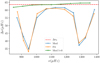 |
Fig. 6. Fitted frequency differences as a function of frequency for an early 1 M⊙ subgiant model, denoted ‘Sub’ in Fig. 5. |
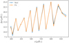 |
Fig. 7. Fitted frequency differences as a function of frequency for a 1 M⊙ model with similar numbers of p-dominated and g-dominated modes. It is denoted ‘Tran’ in Fig. 5. |
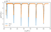 |
Fig. 8. Fitted individual period spacings as a function of frequency for a late 1 M⊙ red giant model. It is denoted ‘RGB’ in Fig. 5. |
Early subgiant. Figure 6 corresponds to an early subgiant model (marked ‘Sub’ in Fig. 5), the first one on the sequence displaying two local minima in the individual period spacing, corresponding to mixed modes. This is the much lower threshold of applicability with regard to the EGGMiMoSA technique. Nonetheless, we observe that it is very efficient at providing a qualitative adjustment of the data. Both the shape and position of individual bumps are properly accounted for. However, we note a slight offset in the bump height around a frequency of 1000 μHz. This offset is similar in amplitude to the error made by assuming the large separation of radial modes to be constant even though it presents a slight dependency with the frequency. This is illustrated by the dashed red line, corresponding to the constant estimate of the large separation of radial modes obtained with WhoSGlAd (Farnir et al. 2019), compared to the local value in green. We observe that the offset between the green and red curves is similar to that between the blue and orange ones.
Late subgiant. We represent a model presenting a comparable amount of pressure dominated modes and gravity dominated ones in Fig. 7 (marked ‘Tran’ in Fig. 5). It corresponds to 𝒩 ≃ 1. Although the shape of the spectrum is complex, we find a proper fit to the data. This is possible thanks to the proper estimation of the parameters beforehand.
Evolved red giant. For the more evolved star displayed in Fig. 8, we again observe a very good agreement with the data. However, we note a slight shift in the position of dips towards low frequencies. Furthermore, we also observe that the adjusted dips tend to be shallower than the data suggests. Possible reasons for such discrepancies will be discussed in Sects. 4.3 and 4.4.
3.2. Variation with mass along the evolution
We present in the current section the variation of the parameters of the adjustment with stellar evolution and mass. The models were computed from the beginning of the subgiant phase up to the RGB-bump. The results are displayed in Figs. 9 through 17. To ease the comparison with other works, stellar evolution goes from right to left.
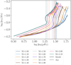 |
Fig. 9. Variation of Δπ1 with Δν0 for different masses, depicted by the colours. The dashed lines correspond to the asymptotic value. The dotted vertical lines correspond to the transition between subgiant and red-giant phases. |
3.2.1. Period spacing, Δπ1
Figure 9 represents the evolution of the period spacing as a function of the large separation of radial modes which decreases with evolution. The large separation is indeed a proxy of the mean density (Ulrich 1986; Farnir et al. 2019) which decreases with evolution during the subgiant and red giant phases. We represent tracks for stellar masses in the range [1.0 M⊙,2.1 M⊙] (0.1 M⊙ step) in different colours. We represent the transition between subgiant and red giant phases (at 𝒩 = 1) by dotted lines. We thus observe that the period spacing decreases with the evolution, at different rates according to the evolutionary phase, the decrease on the subgiant phase being the steepest.
We first note that our computations in Fig. 9 qualitatively agree with the observations of Mosser et al. (2014, see Fig. 1). This confirms that subgiant and red-giant stars occupy distinct regions in a seismic HR diagram. We also note an excellent agreement between the fitted period spacing and its asymptotic value, Δπ1, as, represented by dashed lines (see also Lagarde et al. 2016). Assessing the normalised difference between the fitted and asymptotic values of the large separation, given by  , we observe that it never exceeds 0.2% on the red-giant phase. On the subgiant phase, this difference is greater and decreases as the star evolves. It is below 10−15% at the beginning of the subgiant phase and quickly drops below 5−10%. This demonstrates that as ng increases, the validity of the asymptotic analysis improves. Finally, only a few models exceed the 15% disagreement and they correspond to models with only two g-dominated modes, which stands as the very limit of applicability of our technique. This suggests that the adjusted value is a valid proxy of the asymptotic one. This agreement demonstrates that, although the asymptotic approximation is questionable for g-dominated modes in the subgiant phase (the number of nodes of the g-dominated mode eigenfunction in the buoyancy cavity is ng ∼ 3 in an early subgiant, and its wavelength is thus large), it globally yields valid results. Using the asymptotic expression in Eq. (5), we can crudely estimate that Δπ1 is about inversely proportional to the maximum of the Brunt-Väisälä frequency in the radiative region, which was shown by Pinçon et al. (2020) to be approximately proportional to the square root of the helium core density. The evolution of the helium core density as a function of its mass is plotted in Fig. 10 for different stellar masses. During these stages, the helium core mass increases as Δν decreases. We can thus see that the helium core density progressively increases during evolution, leading to the global decrease in the period spacing, as expected.
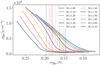 |
Fig. 10. Evolution of the helium core density as a function of its mass. The colours and different line styles have the same indications as in Fig. 9. |
We further note that the subgiant tracks in Fig. 9, corresponding to different masses, are separated to a significant extent. This trend with the stellar mass can again be explained by the dependence of the helium core density on the stellar mass during the subgiant branch as illustrated in Fig. 10. We see in Fig. 9 that the Δπ1 separation between successive tracks is much larger than the typical observed relative uncertainties from Appourchaux (2020), which are smaller than 1% in most cases. This demonstrates that the measure of both Δν0 and Δπ1 should allow us to infer the mass of an observed star with a precision much better than 0.1 M⊙. Consequently, because the age of a subgiant star is dominated by the duration of the main sequence phase, which is a function of the mass, we may in turn constrain the stellar age. This holds great promises for the accurate characterisation of stellar populations. To further demonstrate that the age of a subgiant may indeed be constrained by the measure of Δν0 and Δπ1, we display in Fig. 11, the evolution of the asymptotic period spacing, Δπas, with Δν0 along the subgiant phase. The colour gradient corresponds to the stellar age. We observe that individual tracks indeed represent distinct ages. We also show iso-radius values with the black symbols. Models with 2R⊙ are symbolised by a diamond, models with 3R⊙ by a pentagon and those with 4R⊙ by a star. We observe that measuring both Δπ1 and Δν0 allows us to position a star on this diagram and to constrain its mass, radius and age at a given metallicity. Nevertheless, assuming the duration of the main sequence to be mainly a function of the stellar mass only holds when there is no overshooting during this phase, as is the case for solar-like stars. However, stars with a mass greater than ∼1.2 M⊙ have a convective core, and the overshooting may therefore impact the inferred age. For example, Noll et al. (2021) demonstrated in the specific case of the KIC10273246 subgiant that models with a finite amount of overshooting are in better agreement with observed data that models without overshooting. Including the effect of overshooting will thus be mandatory in more quantitative studies that will follow the preliminary exploratory work presented here.
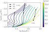 |
Fig. 11. Variation of Δπ1, as with Δν0 on the subgiant phase for different masses. The colour gradient represents the age. The black symbols correspond the models at fixed radius. The diamonds correspond to models of 2R⊙, pentagons to 3R⊙, and stars to 4R⊙. |
In red giants with masses ≲1.8 M⊙, we see in Fig. 9 that the evolution of Δπ1 as a function of Δν converges to a degenerate track. This degeneracy is actually the result of the electron degeneracy in the helium core at these low masses. In these evolved stars, the density contrast between the core and the envelope is such that the mass of the envelope is negligible compared to that of the core. Therefore, we may show by homology that the properties of the shell are determined by the mass and radius of the helium core (Refsdal & Weigert 1970; Kippenhahn et al. 2012). Furthermore, because of the central electron degeneracy, the mass and radius of the core are related and the density of the core is a function of the core mass only. As a consequence, the evolution of the helium core density, in these stars with a degenerate core, should be independent of the total stellar mass and vary only with the mass of the helium core. In particular, this is what we observe in Fig. 10. The low-mass tracks indeed converge to an identical evolution once the transition to the red-giant phase, represented by the dotted vertical lines, has been crossed. The consequence of this relation between the core mass and radius is that the properties of the shell are solely determined by the mass of the helium core. The temperature and luminosity of the shell, which, in turn determine the total luminosity, are then only a function of the mass of the core. As the effective temperature is almost constant on the red-giant branch, the stellar radius thus also predominantly depends on the mass of the core. This is also true for the mean density,  , as it is predominantly a function of the stellar radius. Consequently, the same goes for the large frequency separation Δν that is a proxy of the mean density. This results in a helium core density and a density contrast
  , with ρc the central density, which only depend on the mass of the helium core. These quantities are therefore degenerate as well as a function of the stellar mass for low mass stars with a degenerate core. This is indeed what we observe in Figs. 10 and 12. The consequence of this degeneracy in the core helium density as a function of Δν is the degeneracy in period spacing observed in Fig. 9. Finally, as the degeneracy is lifted in red-giant stars with masses ≳1.8 M⊙, it is theoretically possible to constrain the mass, radius and age of these stars by measuring Δν0 and Δπ1, similarly to the case of the subgiants. However, in practice, it might not be possible to observe such stars as they evolve fast.
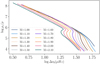 |
Fig. 12. Evolution of the ratio of the central density to the mean stellar density as a function the large separation of radial modes. The colours represent different total stellar masses, as in Fig. 9. |
3.2.2. Pressure offset, ϵp
Figure 13 shows the evolution of the pressure offset as a function of 𝒩, which increases with evolution. From now on, we restrict the sample of masses to a sub-sample (1.0, 1.2, 1.5 and 1.8 M⊙) for better clarity. The same trend is followed by models with masses above 1.8 M⊙. The first striking feature is that there exist two regimes, depending on the evolution stage. During the subgiant phase, we observe that ϵp mostly displays an increasing trend, of which the slope as a function of 𝒩 increases with mass. This increase is followed by a steady decrease along the red giant phase with a slope that is independent of the mass. This is in qualitative agreement with the measured evolution from (Mosser et al. 2013, Fig. 7). We note that their measurements are shifted up by 0.5. This is to be expected as they consider radial modes while we consider l = 1 dipolar modes, which introduces a shift of l/2.
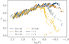 |
Fig. 13. Variation of ϵp as a function of 𝒩. The dashed line correspond to the value estimated with WhoSGlAd on the radial modes. |
We further investigate the two apparent regimes in the evolution of the pressure offset. As it represents the phase lag induced at the boundaries of the pressure cavities, we expect its behaviour to be influenced by their properties. As a consequence, we display in Fig. 14 the density contrast compared to the inner sphere at the lower boundary of the pressure cavity, corresponding to the outer edge of the evanescent region. The local density contrast is defined in Takata (2016) by:
 (18)
(18)
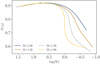 |
Fig. 14. Variation of the density contrast compared to the inner encapsulated sphere at the outer edge of the evanescent region, r2, as in Fig. 9. |
which compares the local density ρ and local mean density  , with m(r) the mass encapsulated by the sphere of radius r. As an example, a value of J = 0.7 means the inner sphere is in average three times denser than the local layer whereas a value of J = 0.9 means the inner sphere is, on average, ten times denser. As the density contrast compared to the inner sphere tends to zero, J tends towards unity. We observe that the density contrast at the outer edge of the evanescent region, r2, is moderate and strongly varies with the mass in the subgiant phase. Then, all the tracks converge towards a similar and high density contrast during the red giant phase (i.e., J ∼ 0.9). This matches the observations for the pressure offset, indicating that the pressure offset holds an information about the density contrast and the structure in the evanescent region. Indeed, Pinçon et al. (2020) showed that the structure of the intermediate evanescent region behaves as power laws of the radius when the density contrast between the core and the evanescent region is large, independently of the stellar mass. This also goes for the Brunt-Väisälä and Lamb frequencies, In contrast, the structure deviates from such a configuration for lower core-envelope density contrast as observed in subgiant stars (see also discussion in Sect. 3.2.4). This suggests that the evolution of the core-envelope density contrast between the subgiant and the red giant branches is the main responsible for the different regimes observed in the pressure offset.
In Fig. 13, during the red giant phase, we observe discontinuities, that result in a seesaw behaviour. This is a direct consequence of the set of modes considered and does not question the quality of the adjustment. Indeed, for such an extended evolution, we may not consider a fixed set of modes, that is, of fixed radial orders. As a consequence, the set shifts towards lower pressure modes orders and discontinuities in the evolution are representative of this shift. Such an effect is discussed in more details in Sect. 4.1.
In this figure, we also represent (as dashed lines) the ϵp, 0 value retrieved for the radial modes via WhoSGlAd. The displayed values account for the l/2 shift in value compared with dipolar modes. We observe that the trends of radial and dipolar modes are in excellent agreement, with a slight offset for the most evolved stars. This illustrates that it is a proper estimate for the pressure offset of the dipolar mixed modes. The seesawing of the radial value of ϵp further demonstrates that this is not caused by any improper convergence of the technique.
In addition, we note that the behaviour is rather erratic during the subgiant phase. This may be a direct consequence of the need to include higher order contributions to the pressure phase, θp, because of the extended set of modes. This aspect is further discussed in Sect. 4.4.
3.2.3. Gravity offset, ϵg
Figure 15 represents the evolution of ϵg with νmax (to ease the comparison with Pinçon et al. 2019, Fig. 4). This is, to our knowledge, the first representation of the gravity offset on a grid of models from the subgiant phase to the red giant phase. As for the case of the pressure offset, we observe two regimes, each depending on the evolutionary phase. We expect that this also stems from the qualitative difference in the evolution of the density contrast in the evanescent region.
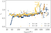 |
Fig. 15. Variation of ϵg as a function of νmax for different masses. |
On the red giant branch, when comparing our results with Fig. 4 of Pinçon et al. (2019) (which confronts their asymptotic computations with observations from Mosser et al. 2018) the agreement is convincing. We must bear in mind that we include an additional 1/2 term in the θg phase compared to their study. As a consequence, the values of ϵg we measure will be shifted up of that same factor compared to theirs. Indeed, in the red giant phase, we observe a plateau at a value of approximately 0.75 of the gravity offset. Accounting for the shift in values of 0.5, this is in excellent agreement with their observation of a plateau at an approximate value of 0.25. This plateau is then followed by a sudden drop of the gravity offset happening in the range of νmax ∈ [50 μHz,110 μHz].
The constant value of the gravity offset during the first part of the red giant branch comes from the fact that, as mentioned earlier, the profiles of the Brunt-Väisälä and Lamb frequencies may be assumed to be parallel and represented by a power-law of radius in the evanescent region because of the high density contrast between the core and the surface. The slope of the Brunt-Väisälä frequency is then constant and determines the gravity offset value. As the star evolves, νmax decreases along with the set of excited modes. Therefore, the evanescent region moves outwards, up to the point where it penetrates the convective zone. The Brunt-Väisälä frequency then suddenly drops. Both frequencies can no longer be considered parallel to one another. The gravity offset then drops, as observed in Fig. 15 and predicted by Pinçon et al. (2019).
In the subgiant phase, we first note that the evolution of ϵg depends on the stellar mass. Similarly to the pressure offset, we expect this dependence to stem from the low and mass-dependent density contrasts displayed by these stars in the evanescent region (see Fig. 14), in opposition to the high and almost mass-independent density contrasts in red giant stars. We also note that the behaviour is less regular than in the red giant phase. However, individual spectra are properly adjusted, as illustrated in Fig. 6 for the most extreme case. We thus expect this effect to either results from structural features or the necessity to extend the asymptotic formulation to higher orders. Another feature in the subgiant phase is the apparent oscillation for low-mass stars, which should be caused by variations in the evanescent region.
Finally, similarly to the case of the pressure offset, we note a seesaw behaviour. This is again a consequence of the varying set of modes. This will be addressed in the discussion (Sect. 4.1).
3.2.4. Coupling factor, q
The evolution of the coupling factor is displayed in Fig. 16. We see that the value of q first increases to a high value in the subgiant phase. This corresponds to the case of a strong coupling (Takata 2016). To be complete, we also note that, for the lowest masses (1.0 M⊙ and 1.2 M⊙), there is a local minimum of the coupling factor before the sharp increase at the end of the subgiant phase. Then it suddenly drops before the red giant phase. Finally, during the red giant phase, the coupling factor steadily decreases from a value of about 0.25 to approximately 0.10, corresponding this time to a weak coupling. Eventually, the value of q further drops by the end of the RGB phase. As our sequences stop at the RGB bump, this drop is not visible for all of them.
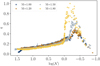 |
Fig. 16. Variation of q as a function of 𝒩 for different masses. |
This predicted evolution of the coupling factor is very similar to observations made by Mosser et al. (2017, namely Fig. 6). As demonstrated by Pinçon et al. (2020) under the assumption that the Brunt-Väisälä frequency and the Lamb frequency are log-parallel, the coupling strength should be a proxy of the width of the evanescent zone; thus the larger the evanescent zone, the lower the coupling. To check whether the width of the evanescent region is correlated with the coupling factor, we display in Fig. 17 the evolution of this relative width at νmax, denoted δev, as a function of the g-dominated modes density. It is defined as:
 (19)
(19)
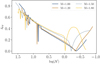 |
Fig. 17. Variation of width of the evanescent zone as a function of 𝒩 for different masses. |
with r1 and r2 the positions of the inner and outer edges of the evanescent region (respectively). For all masses, we indeed observe a global rapid decrease in the size of the evanescent zone during the subgiant phase (with 𝒩 < 1) followed by a steady increase of this size during the red giant phase (with 𝒩 > 1). This coincides with the evolution of the coupling factor. We note that the discontinuities in the evolution on the red giant branch come from the discontinuity in composition at the base of the convective envelope, which, in turn, creates a peak of the Brunt-Väisälä frequency (see for example Cunha et al. 2015).
Regarding the dependence of q with the stellar mass, the two regimes are again observed, as expected from the behaviour of the density contrast in the evanescent region. During the subgiant phase, the coupling factor strongly depends on the mass while, on the red giant branch, the coupling factor is much less sensitive to the stellar mass. In both cases, the same global trend is nevertheless observed: the higher the mass, the lower the q value. Firstly, on the red giant branch, the density contrast in the evanescent region compared to the inner sphere is large enough for the profiles of the Brunt-Väisälä and Lamb frequencies to be assumed to be parallel and the structure of the evanescent region is quite comparable for all the masses at a given value of 𝒩. The width of the evanescent region nevertheless depends slightly on the stellar mass, as seen in Fig. 17, explaining the slight dependence on q observed in Fig. 16 on the red giant branch. Only the position of the ultimate drop of the coupling factor by the end of the sequences appears to be significantly affected by the stellar mass. However, as we restricted ourselves to models before the luminosity bump, this drop is not visible for every track. Secondly, on the subgiant branch, the density contrast is moderate and depends on the stellar mass (see Fig. 14). Because of this lower density contrast than on the red giant branch, the Brunt-Väisälä profile does not follow a simple power-law relation with the radius and may not be assumed to be parallel to the profile of the Lamb frequency. This impacts the evolution of the width of the evanescent region for the different masses, as shown in Fig. 17, and thus explains the significant mass dependence of the coupling factor on the subgiant branch. We even note that the 1.8 M⊙ model exhibits an oscillation with regard to the size of its evanescent region. Indeed, both critical frequencies may cross in this model. As the star evolves, νmax decreases. It therefore reaches this crossing of the frequencies, corresponding to a very narrow evanescent region. Then, as the star continues to evolve, the evanescent region increases in size again. Furthermore, as the frequency profiles also evolve with time (mainly due to the evolution of the density contrast), the point at which they cross may evolve as well and other minima of the width of the evanescent zone may occur, as we observe in Fig. 17. This phenomenon will be further discussed in Pinçon et al. (in prep.).
3.3. Variation with chemical composition along the evolution
To study the impact of the chemical composition on the fitted parameters, we computed several tracks for a 1 M⊙ star with different initial hydrogen and metals abundances. We consider pairs of initial hydrogen and metal abundances in X0 ∈ [0.68,0.72] and Z0 ∈ [0.011,0.019]. The results are shown in Figs. 18–21 for Δπ1, ϵp, ϵg and q, respectively. In Fig. 18, we observe that the several tracks for Δπ1 are almost indistinguishable from one another during the red giant phase. Only a small difference is visible on the subgiant phase. Nevertheless, thanks to a close inspection of our Fig. 18, alongside Fig. 1 of Farnir et al. (2019), we expect that an improper determination of the metallicity will impact the inferred mass in a similar way as it does in the main sequence case. Indeed, at fixed Δπ1 and Δν0 values, a variation of 0.008 in Z0 could change the estimated mass of about 0.1 M⊙. This suggests that, in addition to the measurements of Δν and Δπ1, a spectroscopic measurement of the composition will be necessary to a good determination of the mass, radius and age of subgiant stars. Indeed, the initial composition may impact the inferred stellar mass, thus the inferred age. Regarding ϵp, we do not note any significant impact of the chemical composition on the evolution of this indicator, as illustrated in Fig. 19. Finally, concerning q and ϵg, we note in Figs. 20 and 21 that only the position (in either νmax or log 𝒩) of the drop in the values of ϵg and q just before the luminosity bump is significantly affected by the composition. As shown by Pinçon (2020), this likely results from a modification of the position of the base of the convective envelope.
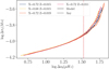 |
Fig. 18. Variation of Δπ1 as a function of Δν0 for 1 M⊙ models with several compositions, represented by the colours. The dashed lines correspond to the asymptotic values and the vertical dotted lines to the transition at 𝒩 = 1. |
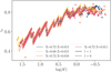 |
Fig. 19. Variation of ϵp as a function of 𝒩 for 1 M⊙ models with several compositions, represented by the colours. The dashed lines correspond to the values computed with WhoSGlAd on the radial modes. |
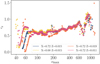 |
Fig. 20. Variation of ϵg as a function of νmax for 1 M⊙ models with several compositions, represented by the colours. |
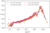 |
Fig. 21. Variation of q as a function of 𝒩 for 1 M⊙ models with several compositions, represented by the colours. |
The impact of the metallicity on the measured value of the period spacing and coupling factor has already been studied by Jiang et al. (2020). In this work, they looked at the evolution of these indicators on a grid of red-giant models, but their fits were made around a fixed value of the pressure radial order np only. While they also observe that there is no significant impact of the metallicity on the evolution of Δπ1, they note a slight impact of the metallicity on the rate of decrease of q. A close look at their Fig. 9 also seems to indicate that this dependency with metallicity mostly appears for the youngest stars. The individual trends seem to settle to a common one as the stellar evolution goes on during the red giant branch. Nevertheless, we do not observe such distinction with the composition. A possible reason for this difference might stem from the fact that they consider the coupling factor to depend on the radial order, np, and represent its evolution following specific modes; whereas we consider the coupling factor to be constant over the spectrum with a typical set of frequencies representative of the observations all along the subgiant and red giant branches. This is further discussed in Sect. 4.4.
Finally, what is striking in Figs. 18–21 is that some subtle features are present for every composition considered. For example, looking at the evolution of the gravity offset in Fig. 20, it stands out that the oscillation present on the subgiant phase is present for all the compositions. Furthermore, in Fig. 21, we also observe that the local minimum in the coupling factor, right before the transition at 𝒩 = 1, is present for every track. This might result from the fact that the changes in composition considered might not significantly affect the evolution on the subgiant phase and, therefore, the evolution of the indicators during this phase. Another striking feature is the homology between the track with X0 = 0.68 and Z0 = 0.015 and the one with X0 = 0.72 and Z0 = 0.011. The tracks are almost identical.
Overall, we may assert that the indicators are degenerate with the chemical composition on the red giant phase, except for the latest stages of evolution: for instance the drops in ϵg and q before the luminosity bump.
4. Discussion
In the present section, we further discuss the results presented in Sect. 3 as well as possible improvements of the EGGMiMoSA method.
4.1. Impact of the considered set of modes
In the present paper, we considered modes in the range of the width  around νmax, determined to include at least ten radial modes for the youngest subgiant models (Mosser et al. 2012b; Appourchaux 2020). We immediately see that this range evolves with νmax, both in terms of its central frequency νmax and in the number of modes. As the number of modes is discrete its evolution experiences discontinuities. This creates the saw-like pattern we observe in the pressure and gravity offsets (Figs. 13, 15, 19 and 20). To illustrate this effect, we plot in Fig. 22 the evolution of ϵp for the 1 M⊙ track as well as the mean radial order of pressure modes,
  . This value is divided by 15, an arbitrary value, such that ϵp and
  have comparable values. We observe that both behave as a seesaw and that the discontinuities in the values are synchronous along evolution. In the case of the observations, the set of modes also changes with evolution, which should also create the discontinuities we observe theoretically. Nevertheless, when attempting to carry stellar modelling of a given star considering ϵp as a constraint, this will not constitute a problem as the set of modes will be fixed by the observations.
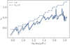 |
Fig. 22. Variation of ϵp with evolution for the 1 M⊙ track. The dashed line represents the variation of the estimation with WhoSGlAd on radial modes and the dot-dashed line the mean pressure radial order of modes considered divided by 15. |
4.2. Generalisation to spectra with holes
When adjusting the spectrum, we assume in this paper that the modes that are adjusted are successive, that is, the difference in radial order between the considered modes, Δng and Δnp, are equal to either 0 or 1. However, when applying the method on observational spectra, it may be the case that some modes are not detected. Consequently, the period and frequency difference formulations in Eqs. (13) and (16) will have to be adapted considering proper values for the Δng and Δnp parameters in these equations. This will thus require that a proper identification of the modes has been carried out.
Moreover, regarding the initial estimation of the parameters to be adjusted, the position and number of holes might be problematic in some specific cases. For example, as we estimated Δπ1 via the maximum of the local period differences in g-dominated spectra, missing several modes in the central region between dips would lead to an underestimation of its value. In addition, the coupling factor is estimated from the ratio between the maximum and minimum of the local difference in period (for g-dominated spectra) or in frequency (p-dominated). Therefore, missing modes close to these minima or maxima might severely impact the initial estimate of q. However, Mosser et al. (2018) have showed that, with Kepler data, g-dominated mixed modes should be below the limit of observability only for evolved giant stars with Δν ≤ 6 μHz, for which only p-dominated mixed modes would be detected. This actually corresponds to the most evolved stars, which are close to the luminosity bump, considered in this study. The number of observed g-dominated modes should increase as we go down the red giant branch, meaning that younger stars should constitute less of a problem. Therefore, it will be necessary in future studies to test the ability of the method to provide correct results in such evolved cases.
4.3. Higher order contributions to the asymptotic formulation
In the present paper, we considered the pressure phase, θp, to depend linearly on the frequency. However, because the set of modes is broad in the case of subgiant stars (about 10Δν wide), the large separation may not be considered to be constant over this interval. As an illustration, its relative variation in the subgiant star considered in Fig. 6 is of about  . Furthermore, the mean value of the pressure radial order is of np ∼ 20 in such stars. As a consequence, the product of both quantities, corresponding to the error made by considering only a linear pressure phase, is on the order of unity. It is therefore not negligible compared to typical observed uncertainties on ϵp. In such a case, the assumed formulation for the pressure phase may not be valid any more. Therefore, it may be necessary to include second-order contributions to this phase. This effect may be so important that it may result in the addition or removal of a p-dominated mode to the set of considered frequencies. Following this discussion, the case of the gravity phase of evolved red-giants naturally comes to mind, as such stars span a large range of gravity radial orders. However, Pinçon et al. (2019) analytically showed that the second order contribution to the gravity phase remains small compared to the current observed uncertainties on the gravity offset for stars typically observed before the luminosity bump.
For the evolved red giant stars, it may again be necessary to include higher order contributions to the pressure phase (Mosser et al. 2013). Indeed, we noted in Fig. 8 that there is a slight shift in the position of the ΔP dips as well as small differences in their exact magnitude. This can now be caused by the fact that the hypothesis that the number of nodes in the pressure cavity is large and thus that the local wavelength is small is not verified for the pressure dominated modes. Indeed, the radial order of p-dominated modes is very low, namely, np ∼ 5.
The inclusion of such higher order contributions to the pressure phase might be necessary to improve the robustness of the method and of the measured seismic indicators. As a consequence, it will be implemented and tested in subsequent papers of this series.
4.4. Frequency dependence of the coupling factor in evolved red giants
Cunha et al. (2019) showed that, for evolved models, the coupling factor may depend on the frequency. This is due to the fact that the evanescent zone has penetrated into the convective zone. As a consequence, the Brunt-Väisälä frequency drops to zero and is no longer log-parallel to the Lamb frequency. The relative width of the evanescent region defined in Eq. (19) may not be considered constant with respect to the frequency any longer. Therefore, the coupling factor may in turn depend on the frequency (Pinçon et al. 2020). To mimic this effect, we binned the oscillation spectrum of the evolved giant presented in Fig. 8 into sub-spectra containing only one dip each. The binned spectrum is shown in Fig. 23. We then fitted individual q values in each sub-spectra. The evolution of the coupling factor as a function of the central frequency of each bin is displayed in Fig. 24. We indeed observe that it may vary with the frequency in an almost linear fashion. Only the coupling factor in the lowest frequency bin strays far from the linear trend. This may result from the asymmetric number of modes around the dip. Finally, we note that the variation of the coupling factor on the spectrum is significant when compared to the constant fitted value. Indeed, while the fitted value is of about 0.12 (comparable to values in the literature, see Mosser et al. 2017), it changes from ∼0.11 to ∼0.22 along the spectrum. This illustrates the necessity to account for its dependency with the frequency in order to properly interpret its value.
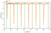 |
Fig. 23. Fitted individual period spacings as a function of frequency for the same red-giant model as in Fig. 8, but the spectrum has been binned for each individual bump. The green vertical dashed lines delimit each bin. |
4.5. Glitches
A further refinement of the technique would be the inclusion of glitches in the formulation used. These glitches are the result of a sharp variation (compared to the wavelength of the incoming mode) in the stellar structure. Their signature is an oscillating feature in the oscillation spectrum. Cunha et al. (2015) showed that buoyancy glitches, caused by a sharp variation in the Brunt-Väisälä frequency, are mainly found for red giant stars at the luminosity bump, at the early phases of helium core burning and at the beginning of helium shell burning. In this paper, we only consider models before the luminosity bump. Therefore, we should not expect the detection of such glitches in these models. Nonetheless, their inclusion will be a necessary step to the application of the EGGMiMoSA method to more evolved stellar models and data. Furthermore, such glitches carry essential information for constraining the stellar cores of giants as well as the transport processes of chemical elements.
Aside from buoyancy glitches, there are the acoustic glitches, found in the pressure part of the spectrum. In the case of red giants, we may observe the signature of the helium glitch, created by the second ionisation zone of helium. Therefore, it holds information about the surface helium content, providing additional constraints to stellar models. The study of such glitches in giant stars has been carried in the past (e.g., Miglio et al. 2010; Dréau et al. 2020). Combining the present method with WhoSGlAd (Farnir et al. 2019) we will be able to retrieve this signature in the p-dominated modes in a robust way. The inclusion of both the buoyancy and acoustic glitches in the dipolar modes will be discussed in subsequent papers of this series.
5. Conclusion
With the aim of defining relevant seismic indicators and relying on a prior modes extraction (e.g., Mosser et al. 2015; Gehan et al. 2018; Appourchaux 2020), we present a method of automated, consistent, robust, and fast adjustment of observed and theoretical mixed-mode oscillation spectra. Theoretical oscillations spectra of low-mass subgiant and red-giant stars are well adjusted, as illustrated in Figs. 6–8.
We explored the probing potential of the mixed-mode parameters (Δν, Δπ1, ϵp, ϵg, and q) as indicators of the stellar structure of subgiant and red giant stars, along a grid of models for masses between 1.0 M⊙ and 1.8 M⊙ (extended to 2.1 M⊙ in the case of Δπ1) and initial chemical compositions in X0 ∈ [0.68,0.72] and Z0 ∈ [0.011,0.019]. Overall, the evolution of the indicators displays clear trends and the chemical composition has only a slight impact. In contrast, we note that the evolution of the parameters with the mass follows two regimes, depending on the evolutionary stage of the star.
During the subgiant phase, because of a moderate core-envelope density contrast, the mixed-mode parameters evolve differently with Δν according to the stellar mass. Notably, the evolution of Δπ1 in subgiants is such that it may be used, combined with Δν and a proper measurement of the metallicity, to infer the stellar mass, radius and age (Fig. 11). We also demonstrate that the asymptotic period spacing tightly agrees with the fitted one. This came as a surprise as the contribution of the gravity modes departs from the asymptotic regime for these stars.
As the stars evolve to the red giant phase, the core-envelope density contrast becomes large. As a consequence, the structure of the evanescent region is almost independent of the stellar mass and the evolutions of the pressure offset, gravity offset, and coupling factor as a function of Δν are not really affected by the stellar mass in this phase. We showed that this is also true for Δπ1 in stars with masses ≲1.8 M⊙ because of the core electron degeneracy, which makes the helium core density quasi independent of the stellar mass at a given value of Δν. Above this threshold, the electron degeneracy is lifted and the evolution of Δπ1 again depends on the mass. Observing stars in that region would therefore allow us to constraint their masses, radii, and ages, similarly to the case of subgiants. However, such stars evolve swiftly and might not be observed.
Here, we provide the first depiction, to our knowledge, of the gravity offset evolution along a grid of models during both the subgiant and red giant phases. The evolution during the red-giant phase agrees with the observations of Mosser et al. (2018) and the asymptotic computations from Pinçon et al. (2019). As the gravity offset corresponds to the phase lag of the g-dominated modes induced at the inner edge of the evanescent region, we expect it should hold information about this region. However, some issues remain to be tackled as the behaviour of this indicator remains erratic in the subgiant phase.
The evolution of the coupling factor along our grid of models also qualitatively agrees with the observations of Mosser et al. (2017). We also show, based on the study of Pinçon et al. (2020), that its evolution is concordant with that of the width of the evanescent region (see Fig. 17).
Owing to the use of the asymptotic formulation and appropriate estimation of the mixed-mode parameters, the EGGMiMoSA technique offers a robust and fast1 adjustment of the mixed-mode spectra displayed by subgiant and red giant stars. Furthermore, we also plan on extending the method to include refinements of the asymptotic formulation such as higher order contributions and glitches. Finally, we expect that the technique would represent a great asset to the automated treatment of large samples of data as will be generated by spacecrafts such as PLATO (Rauer et al. 2014), which will observe a great number of subgiant stars (core program) and red-giant stars (secondary science program). Indeed, after a proper modes extraction, the measured seismic indicators can be used as constraints on stellar models to automatically compute stellar parameters with model search algorithms such as AIMS (Rendle et al. 2019).
Computation times are much smaller than those necessary to compute theoretical adiabatic frequencies.
We recall that Δnp < 2 between xj + 1 and xj − 1 when 𝒩 > 1, in a similar way that Δng > −2 when 𝒩 < 1.
Acknowledgments
M. F. is supported by the FRIA (Fond pour la Recherche en Industrie et Agriculture) – FNRS PhD grant. C. P. is supported by the F. R. S – FNRS as a Chargé de Recherche.
References
- Aizenman, M., Smeyers, P., & Weigert, A. 1977, A&A, 58, 41 [NASA ADS] [Google Scholar]
- Appourchaux, T. 2020, A&A, 642, A226 [NASA ADS] [CrossRef] [EDP Sciences] [Google Scholar]
- Appourchaux, T., Chaplin, W. J., García, R. A., et al. 2012, A&A, 543, A54 [NASA ADS] [CrossRef] [EDP Sciences] [Google Scholar]
- Baglin, A., Auvergne, M., Barge, P., et al. 2009, in Transiting Planets, eds. F. Pont, D. Sasselov, M. J. Holman, et al., IAU Symp., 253, 71 [Google Scholar]
- Bedding, T. R., Mosser, B., Huber, D., et al. 2011, Nature, 471, 608 [Google Scholar]
- Benomar, O., Bedding, T. R., Stello, D., et al. 2012, ApJ, 745, L33 [NASA ADS] [CrossRef] [Google Scholar]
- Borucki, W. J., Koch, D., Basri, G., et al. 2010, in American Astronomical Society Meeting Abstracts #215, BAAS, 42, 215 [Google Scholar]
- Cunha, M. S., Stello, D., Avelino, P. P., Christensen-Dalsgaard, J., & Townsend, R. H. D. 2015, ApJ, 805, 127 [Google Scholar]
- Cunha, M. S., Avelino, P. P., Christensen-Dalsgaard, J., et al. 2019, MNRAS, 490, 909 [Google Scholar]
- Deheuvels, S., & Michel, E. 2011, A&A, 535, A91 [NASA ADS] [CrossRef] [EDP Sciences] [Google Scholar]
- Deheuvels, S., Doğan, G., Goupil, M. J., et al. 2014, A&A, 564, A27 [NASA ADS] [CrossRef] [EDP Sciences] [Google Scholar]
- Dréau, G., Cunha, M. S., Vrard, M., & Avelino, P. P. 2020, MNRAS, 497, 1008 [CrossRef] [Google Scholar]
- Dupret, M. A., Belkacem, K., Samadi, R., et al. 2009, A&A, 506, 57 [NASA ADS] [CrossRef] [EDP Sciences] [Google Scholar]
- Farnir, M., Dupret, M. A., Salmon, S. J. A. J., Noels, A., & Buldgen, G. 2019, A&A, 622, A98 [NASA ADS] [CrossRef] [EDP Sciences] [Google Scholar]
- Frandsen, S., Carrier, F., Aerts, C., et al. 2002, A&A, 394, L5 [NASA ADS] [CrossRef] [EDP Sciences] [Google Scholar]
- Gehan, C., Mosser, B., Michel, E., Samadi, R., & Kallinger, T. 2018, A&A, 616, A24 [NASA ADS] [CrossRef] [EDP Sciences] [Google Scholar]
- Gough, D. O. 1986, Highlights Astron., 7, 283 [CrossRef] [Google Scholar]
- Hekker, S., & Christensen-Dalsgaard, J. 2017, A&ARv, 25, 1 [NASA ADS] [CrossRef] [EDP Sciences] [Google Scholar]
- Hekker, S., Elsworth, Y., & Angelou, G. C. 2018, A&A, 610, A80 [NASA ADS] [CrossRef] [EDP Sciences] [Google Scholar]
- Jiang, C., & Christensen-Dalsgaard, J. 2014, MNRAS, 444, 3622 [NASA ADS] [CrossRef] [Google Scholar]
- Jiang, C., Cunha, M., Christensen-Dalsgaard, J., & Zhang, Q. 2020, MNRAS, 495, 621 [Google Scholar]
- Kippenhahn, R., Weigert, A., & Weiss, A. 2012, Stellar Structure and Evolution (Heidelberg: Springer, Berlin Heidelberg) [Google Scholar]
- Lagarde, N., Bossini, D., Miglio, A., Vrard, M., & Mosser, B. 2016, MNRAS, 457, L59 [NASA ADS] [CrossRef] [Google Scholar]
- Miglio, A., Chiappini, C., Mosser, B., et al. 2017, Astron. Nachr., 338, 644 [NASA ADS] [CrossRef] [Google Scholar]
- Miglio, A., Montalbán, J., Carrier, F., et al. 2010, A&A, 520, L6 [NASA ADS] [CrossRef] [EDP Sciences] [Google Scholar]
- Montalbán, J., Miglio, A., Noels, A., Scuflaire, R., & Ventura, P. 2010, ApJ, 721, L182 [Google Scholar]
- Montalbán, J., Miglio, A., Noels, A., et al. 2013, ApJ, 766, 118 [NASA ADS] [CrossRef] [Google Scholar]
- Mosser, B., Goupil, M. J., Belkacem, K., et al. 2012a, A&A, 540, A143 [NASA ADS] [CrossRef] [EDP Sciences] [Google Scholar]
- Mosser, B., Elsworth, Y., Hekker, S., et al. 2012b, A&A, 537, A30 [NASA ADS] [CrossRef] [EDP Sciences] [Google Scholar]
- Mosser, B., Michel, E., Belkacem, K., et al. 2013, A&A, 550, A126 [NASA ADS] [CrossRef] [EDP Sciences] [Google Scholar]
- Mosser, B., Benomar, O., Belkacem, K., et al. 2014, A&A, 572, L5 [NASA ADS] [CrossRef] [EDP Sciences] [PubMed] [Google Scholar]
- Mosser, B., Vrard, M., Belkacem, K., Deheuvels, S., & Goupil, M. J. 2015, A&A, 584, A50 [NASA ADS] [CrossRef] [EDP Sciences] [Google Scholar]
- Mosser, B., Pinçon, C., Belkacem, K., Takata, M., & Vrard, M. 2017, A&A, 600, A1 [NASA ADS] [CrossRef] [EDP Sciences] [Google Scholar]
- Mosser, B., Gehan, C., Belkacem, K., et al. 2018, A&A, 618, A109 [NASA ADS] [CrossRef] [EDP Sciences] [Google Scholar]
- Noll, A., Deheuvels, S., & Ballot, J. 2021, A&A, 647, A187 [EDP Sciences] [Google Scholar]
- Osaki, Y. 1971, PASJ, 23, 485 [NASA ADS] [Google Scholar]
- Pinçon, C. 2020, in Stars and their Variability Observed from Space, eds. C. Neiner, W. W. Weiss, D. Baade, et al., 313 [Google Scholar]
- Pinçon, C., Takata, M., & Mosser, B. 2019, A&A, 626, A125 [NASA ADS] [CrossRef] [EDP Sciences] [Google Scholar]
- Pinçon, C., Goupil, M. J., & Belkacem, K. 2020, A&A, 634, A68 [CrossRef] [EDP Sciences] [Google Scholar]
- Rauer, H., Catala, C., Aerts, C., et al. 2014, Exp. Astron., 38, 249 [Google Scholar]
- Refsdal, S., & Weigert, A. 1970, A&A, 6, 426 [NASA ADS] [Google Scholar]
- Rendle, B. M., Buldgen, G., Miglio, A., et al. 2019, MNRAS, 484, 771 [Google Scholar]
- Scuflaire, R. 1974, A&A, 36, 107 [NASA ADS] [Google Scholar]
- Scuflaire, R., Montalbán, J., Théado, S., et al. 2008a, Ap&SS, 316, 149 [Google Scholar]
- Scuflaire, R., Théado, S., Montalbán, J., et al. 2008b, Ap&SS, 316, 83 [Google Scholar]
- Shibahashi, H. 1979, PASJ, 31, 87 [NASA ADS] [Google Scholar]
- Takata, M. 2016, PASJ, 68, 91 [NASA ADS] [CrossRef] [Google Scholar]
- Tassoul, M. 1980, ApJS, 43, 469 [Google Scholar]
- Ulrich, R. K. 1986, ApJ, 306, L37 [Google Scholar]
- Vrard, M., Mosser, B., & Samadi, R. 2016, A&A, 588, A87 [NASA ADS] [CrossRef] [EDP Sciences] [Google Scholar]
Appendix A: Bounds of the asymptotic frequency differences
The method presented in Sect. 2 takes advantage of the theoretical bounds of the first and second frequency differences of the asymptotic frequency pattern. On the one hand, the first frequency (resp. period) difference between two consecutive modes normalised by Δν (resp. Δπ1) is always smaller than unity. On the other hand, the second frequency difference in (Eq. (6)) displays values greater than 1 in a p-dominated spectrum while it presents values lower than 1 in g-dominated spectra. In the current section, we mathematically demonstrate these statements.
A.1. Case 𝒩 < 1 over the spectrum
In a first step, we study the properties of the asymptotic frequency pattern focusing on the case where the local g-dominated mode density 𝒩(ν) < 1. Using the expression of the pressure phase (Eq. (2)), we may first rewrite the asymptotic resonance condition (Eq. (1)) as a function of the independent variable x = ν/Δν. In this form, the asymptotic frequency pattern is obtained by solving the implicit relation
![Mathematical equation: $$ \begin{aligned} x = \mathcal{F} (n_p,x) = n_p + \epsilon _p +\frac{1}{\pi } \arctan \left[q \tan \left( \theta _g \left(x\right) \right)\right]\; , \end{aligned} $$](/articles/aa/full_html/2021/09/aa41317-21/aa41317-21-eq36.gif) (A.1)
(A.1)
where np is the pressure radial order and the gravity phase θg (Eq. (3)) is also expressed as a function of the variable x, that is,
![Mathematical equation: $$ \begin{aligned} \theta _g (x) = \pi \left[x \mathcal{N} (x)-\epsilon _g +1/2 \right], \end{aligned} $$](/articles/aa/full_html/2021/09/aa41317-21/aa41317-21-eq37.gif) (A.2)
(A.2)
with 𝒩(x) = (x2ΔνΔπ)−1 the local g-dominated modes density defined in Eq. (4) but rewritten in terms of the x variable.
As an illustration, the ℱ function in the case 𝒩(x) < 1 is plotted as a function of x in Fig. A.1 for different values of np. To plot this figure, we choose Δπ1Δν ≈ 200, which is a typical value for an observed subgiant star. The solutions of the implicit equation in Eq. A.1 are provided by the intersection between the ℱ function and the identity function f(x) = x represented by the solid black line. These solutions are shown as red filled circles. In this figure, a given value of np is associated with a horizontal strip located in the range [np + ϵp − 1/2, np + ϵp + 1/2[ in the vertical axis. In such a horizontal strip, we see that the ℱ function exhibits discontinuities as a function of x. These discontinuities occur at values, xng, which correspond to the frequencies of pure g-modes verifying the condition θg = (ng + 1/2)π with ng ∈ ℕ the gravity radial order. The values of xng are thus provided by
 (A.3)
(A.3)
The positions, xng, for different values of ng are represented by vertical dashed lines in Fig A.1. As the gravity phase θg has a local period in x of 𝒩(x) < 1, it is obvious that two consecutive pure gravity modes are such that: xng − xng + 1 > 1, as confirmed in Fig. A.1. Over a range Ing = ]xng + 1, xng] (referred to as ‘g-subset’) and for a given value of np, we also note that ℱ(np, x) is continuous and monotonically decreasing as a function of x, which can be easily checked by deriving this function with respect to x.
With framework set out thus far, it is now possible to study the bounds of the first and second differences of the solution pattern in a simple way. For the sake of convenience, we start the investigation with the first difference. Firstly, we focussed on a g-subset Ing. Over such an interval, we distinguished three cases:
-
On each subset Inp = [np+ϵp−1/2,np+ϵp+1/2[ (referred to as ‘p-subset’) such that Inp ⊂ Ing, the f function monotonically and continuously increases from np + ϵp − 1/2 to np + ϵp + 1/2. In contrast, the ℱ(np, x) function monotonically and continuously decreases and is such that: np + ϵp − 1/2 < ℱ(np, x) < np + ϵp + 1/2. Therefore, both functions intersect only once and there is only one solution in the p-subset Inp.
-
Over the subset
![Mathematical equation: $ I_{n_p^-}=]x_{n_g+1},n_p^- + \epsilon_p +1/2] $](/articles/aa/full_html/2021/09/aa41317-21/aa41317-21-eq39.gif) , where
, where  is the lowest integer such as
  , according to the continuity and the monotonic behaviour of the ℱ and f functions, we still have only one solution since
  and
and  .
. -
Over the subset
![Mathematical equation: $ I_{n_p^+}=[n_p^+ + \epsilon_p -1/2,x_{n_g}] $](/articles/aa/full_html/2021/09/aa41317-21/aa41317-21-eq44.gif) where
where  is the largest integer such as
  , according to the continuity and the monotonic behaviour of the ℱ and f functions, we again have only one solution since
  and
and 
 .
.
As a result, over a g-subset Ing, each solution is associated with a unique value of np. Now, because  since xng − xng + 1 > 1 when 𝒩 < 1, there are at least two solutions over Ing, and we call xk the solution associated with the pressure radial order
  with
with  . We thus have for each successive solutions
 (A.4)
(A.4)
where the last equality comes from the definition of the phase function (Eq. A.1) and the fact that the difference of pressure radial order between two successive solutions is Δnp = np, k + 1 − np, k = 1. Because θg(x) monotonically decreases over Ing, the ℱ function continuously decreases as well and we have:
 (A.5)
(A.5)
such that xk + 1 − xk < 1. Finally, the last case to tackle is when two successive solutions belong to two successive distinct g-subsets Ing and Ing − 1. We have just shown that these two solutions belong to the same p-subset Inp such as xng ∈ Inp. The difference of pressure radial order between these two successive solutions is thus Δnp = 0 and it is trivial to conclude that the difference between the two solutions remains lower than unity. All these findings are well illustrated in the square grey domains in Fig. A.1, which represent the ‘p-domain’ Inp × Inp that contains the solutions of the implicit relation. To summarize this first part, we have thus shown that the difference between two successive solutions of the implicit equation is smaller than unity. Converting this result as a function of the frequency νj (listed in ascending order with respect to the subscript j), we therefore obtain in pressure-dominated spectra such as 𝒩(ν) < 1, such that
 (A.6)
(A.6)
which in terms of period Pj = 1/νj is equivalent to
 (A.7)
(A.7)
because 𝒩(x) < 1 in the present case. Moreover, we have shown that the difference of pressure radial orders between two successive modes is either equal to unity when the modes belong to the same g-subset associated with a unique gravity radial order ng (i.e., Δnp = 1 and Δng = 0), or equal to zero when the modes belong to two successive distinct g-subsets associated with successive gravity radial orders ng and ng − 1, respectively (i.e., Δnp = 0 and Δng = −1).
Secondly, we now search the bounds of the second difference between two solutions xj + 1 and xj − 1. According to the previous paragraph, we always have xj + 1 − xj < 1 when 𝒩 < 1, so that the upper bound of the second difference is directly xj + 1 − xj − 1 < 2. Regarding the lower bound, we first note that when the three considered solutions, xj − 1, xj, and xj + 1, are part of the same g-subset Ing, they are associated with successive values of the pressure radial order; thus, it is obvious that 1 < xj + 1 − xj − 1 since Δnp = np, j + 1 − np, j − 1 = 2. When the three solutions are spread over two g-subsets, such that xj ∈ Ing and xj + 1 ∈ Ing − 1, we cannot directly draw a conclusion. To demonstrate that the result also holds in that case, we define the functions around the pure g-mode xng:
![Mathematical equation: $$ \begin{aligned} \tilde{\mathcal{F} }\left(n_p,x;x_{n_g} \right)&= \ n_p + \epsilon _p \\ \nonumber&+ \frac{1}{\pi }\arctan \left[q \tan \left\{ \tilde{\theta _g}\left(x;x_{n_g} \right) \right\} \right] \; , \end{aligned} $$](/articles/aa/full_html/2021/09/aa41317-21/aa41317-21-eq57.gif) (A.8)
(A.8)
and
 (A.9)
(A.9)
where we recall that θg(xng) = π(1/2 + ng). In an analogous way to the previous steps, we define the three consecutive solutions  ,
,  , and
, and  around xng of the new implicit equation:
 (A.10)
As shown previously, the solutions  and
and  around xng are respectively associated with the radial orders np, j + 1 and np, j − 1 = np, j + 1 − 1, as consecutive solutions on both sides of xng verify Δnp = 0. In this case, the
  function has a period of 1 and it is obvious that
  . To go further, we then express the θg phase in Eq. A.2 as
 (A.11)
where the second equality comes from Eq. (A.3). By comparing Eq. (A.11) with the definition of  in Eq. (A.10), we can determine that:
 (A.12)
since  and 𝒩(xng) < 1, which implies that
 (A.13)
In other words, this means that the identity function and the ℱ function do not intercept for  inside the considered interval Inp, j + 1 ∩ Ing − 1, so that they will necessarily intercept at a higher value (since we have shown before that there is a unique solution in such an interval), that is,
 (A.14)
Similarly, for  , we have:
 (A.15)
implying
 (A.16)
This means that the identity function and the ℱ function do not intercept for  inside the considered interval Inp, j − 1 ∩ Ing, so that they will necessarily intercept at a lower value, that is,
 (A.17)
As a result, we find that:
 (A.18)
In summary, we thus conclude that for 𝒩 < 1, the second frequency difference is bounded, such that:
 (A.19)
A.2. Case 𝒩 > 1 over the spectrum
In a g-dominated spectrum, the analysis can be put in a similar form to the case treated in App. A.1 if we apply the following substitutions
 (A.20)
Indeed, in the case 𝒩 > 1, we have 𝒩″ < 1, and it is possible to follow the same reasoning as in the previous section.
One the one hand, for the first difference, when 𝒩 > 1 over the considered spectrum, we obtain:
 (A.21)
 (A.22)
Moreover, the difference of gravity radial orders between two successive modes (i.e., still listed in ascending order with frequency) is either equal to −1 when the modes belong to the same p-subset associated with a unique pressure radial order np (i.e., Δng = −1 and Δnp = 0), or equal to zero when the modes belong to two successive distinct p-subsets associated with successive pressure radial orders np and np + 1, respectively (i.e., Δng = 0 and Δnp = 1).
On the other hand, for the second period difference, we obtain when 𝒩 > 1 over the considered spectrum
 (A.23)
For the second frequency difference, when 𝒩 > 1, we can solely determine:
 (A.24)
where an alternative definition for the g-dominated mode density naturally appears, namely,
 (A.25)
Since  , we have
  over the considered spectrum. As soon as 𝒩′> 2, Eq. (A.24) shows us that δν2, j < 1. In the case 1 < 𝒩′< 2, we can adapt the reasoning made in App. A.1. Indeed, either the solutions xj − 1 and xj + 1 are associated with the same pressure radial order (i.e., Δnp = 0 and Δng = −2) and xj + 1 − xj − 1 < 1, or the difference in np is equal to unity (i.e., with Δng = −1)2. In the second case, this means that the solutions xj − 1 and xj + 1 are located on both sides of a pure g-mode xng. Applying the reasoning as in App. A.1 to determine the bounds of the second frequency difference, we obtain xj + 1 − xj − 1 < 1 as 𝒩 > 1 in the present case. We therefore conclude that over a spectrum such as 𝒩 > 1, we have
 (A.26)
A.3. Case 𝒩 = 1 somewhere in the spectrum
The last case to tackle is when the two solutions that are compared are located from each side of the transition point x⋆ where 𝒩(x⋆) = 1.
For the first difference, the demonstration is simple. We denote xq (resp. xq + 1) as the largest (the smallest) solution lower (resp. greater) than x⋆. If we note  as the lowest gravity radial order such a
  , we have
  since otherwise
  would not be the highest lowest gravity radial order such that
  as xng − xng + 1 < 1 when 𝒩 > 1. Therefore, we have two cases. If
  , xq + 1 is then necessarily comprised in the same p-subset as xq. If
  , either
  and xq + 1 is then again necessarily comprised in the same p-subset as xq; or
  and xq + 1 then belongs to an adjacent p-subset to that of xq. In all cases, following the same reasoning as in Appendix A.1, we have xj + 1 − xj < 1, which is therefore unconditionally met over the whole spectrum. This is obviously also true for the difference in period.
For the second difference, we consider two solutions xj − 1 and xj + 1 such as xj − 1 < x⋆ and xj + 1 > x⋆. We also consider the solutions of the implicit equation:
 (A.27)
where  is defined in Eqs. A.8. It can be straightforward to see that xj − 1 is solution of Eq. (A.27). By considering the consecutive solutions
  and
and  of Eq. (A.27), we obviously have
  since the
  function has a period of 1. To go further, we then compute from Eq. A.9
 (A.28)
with  defined as in Eq. (A.25). Therefore, if
  , we have
  according to Eq. (A.28). This means that the
  function and the identity function intercept at higher values than xj + 1. In other words,
  , and thus xj + 1 − xj − 1 < 1. Conversely, if
  , we have
  . This means that the
  function and the identity function can intercept at lower values than xj + 1. In other words,
  , and thus xj + 1 − xj − 1 > 1.
Therefore,  appears to be a relevant proxy of the g-dominated modes density over the whole spectrum. Indeed, we remind that in the previous cases considered in Sects. A.1 and A.2, when 𝒩(νj + 1) > 1, then
  and δν2, j < 1, and when 𝒩(νj − 1) < 1, then
  and δν2, j > 1. Adding in the results of the present section, we thus conclude that over the whole spectrum:
 (A.29)
where sgn() denotes the sign function.
A.4. Illustration
We illustrate in Fig. A.2 the evolution of the second difference (Eq. (6)) with the reduced period, obtained by solving Eq. (1). We show this evolution for two choices of the coupling factor q = 0.1 and q = 0.4 in red and blue, respectively. We also show, as dashed lines, the evolution of the alternate definition for the g-dominated modes density 𝒩′ in Eq. (A.25). We observe that 𝒩′ and the second frequency difference cross at a value of 1, as expected from the previous sections. As a consequence, we may locate the transition where 𝒩j = 1 using the second frequency difference.
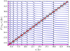 |
Fig. A.1. Evolution of the phase function with the frequency over the large speration. The phase function for different pressure radial orders is represented in blue. The straight line represents the identity function f(x) = x. Its intersections with the phase function are the solutions, in red. The grey square domains represent regions of constant np values. The vertical dashed lines are the positions of pure g-modes. The mixed-mode parameters used are q = 0.2 and ΔνΔπ1 = 200 |
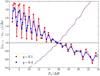 |
Fig. A.2. Second frequency difference δν2 as a function of the normalised period of mixed modes (dots). The red and blue colours are for q = 0.1 and q = 0.4, respectively. It is plotted for a typical value of ΔνΔπ1 = 200. The corresponding dashed curves show the evolution of 𝒩′. |
Appendix B: Deriving ζ′
With analogous reasoning as in Mosser et al. (2015), we may express the variation of frequency with the mixed-mode radial order, n = np − ng. Assuming the spectrum to be dominated by the pressure modes, 𝒩 ≪ 1, we consider that the frequency of a mixed mode experiences a perturbation from the evenly space frequencies, η. We write:
 (B.1)
(B.1)
Because of periodicity, when introducing this relation in the phase of pressure modes, θp (Eq. (2)), tanθp becomes
![Mathematical equation: $$ \begin{aligned} \tan \left[\pi \left(\frac{\eta }{\Delta \nu } - \epsilon _p\right)\right]. \end{aligned} $$](/articles/aa/full_html/2021/09/aa41317-21/aa41317-21-eq120.gif) (B.2)
(B.2)
The derivation of Eq. (1) with respect to n, assuming the five mixed-mode parameters to be constant with n, then yields
 (B.3)
(B.3)
Finally, using the relation  (obtained from Eq. (1)), using η = ν − nΔν, and the definition of the g-dominated modes density evaluated in ν (Eq. (4)), we retrieve the final expression:
![Mathematical equation: $$ \begin{aligned} \frac{d \nu }{d n} = \Delta \nu \left[1 + \frac{q\mathcal{N} }{\cos ^2 \theta _g + q^2 \sin ^2\theta _g} \right]^{-1}. \end{aligned} $$](/articles/aa/full_html/2021/09/aa41317-21/aa41317-21-eq123.gif) (B.4)
(B.4)
We note that θg and 𝒩 in Eq. (B.4) are two functions of frequencies provided by Eqs. (3) and (4).
Appendix C: Radial order difference between successive modes
Based Eq. (13), along with the fact that between two g-dominated modes there may exist a p-dominated mode, it is not obvious that Δng should be equal to zero or one. By carefully studying the behaviour of first and second frequency differences, Appendix A provides a justification for its value. Nevertheless, to focus only on the Δng parameter, we follow a slightly different but equivalent approach in the present section.
From Appendix A, we know that the local value of the period spacing is at most equal to the asymptotic value Δπ1. Furthermore, from the ordering of frequencies, ΔPi must be positive. We thus have (from Eq. (13)):
 (C.1)
(C.1)
Also, we have that θp is an increasing function of the frequency (see Eq. (2)), thus θp, i < θp, i + 1. As the arctan function is continuous and monotonous and the tan function is continuous and monotonous over a given interval θp ∈ [kπ−π/2,kπ+π/2], k ∈ ℕ, the ψi = arctan(tanθp, i/q) is continuous and monotonous over the same interval. In addition, in such an interval, ψi increases with θp, i. Thus, Δψi < 0. Using the definition of the arctan function, we know that ψ ∈ ]−π/2,π/2[ and Δψi/π must be greater than −1. We may thus conclude that:
 (C.2)
(C.2)
and, as ng only takes integer values, Δng = 1. This demonstration does not hold in the case where two successive modes span over different intervals θp ∈ [kπ−π/2,kπ+π/2], k ∈ ℕ, the tan function is discontinuous. In that case, Δψi > 0 and it is necessary to have Δng = 0 to ensure ΔPi/Δπ1 < 1. Physically speaking, this corresponds to the case when we alternate between a g-dominated and a p-dominated mode and this is the pressure radial order that changes, keeping a constant ng value.
Finally, with an analogous reasoning, we may conclude, for the case of p-dominated spectra that Δnp, appearing in Eq. (16), must also equal 1 for two successive p-dominated modes. Again, when two successive modes span over different intervals θg ∈ [kπ−π/2,kπ+π/2], k ∈ ℕ, we alternate between a p-dominated mode and a g-dominated mode, and the gravity radial order changes, keeping in a constant np value.
All Tables
All Figures
|
Fig. 1. Oscillation frequency differences between consecutive modes as a function of the period in the 1 M⊙ subgiant model presented in Table 1. The green horizontal line represents the large separation value calculated for radial modes. The double-sided arrow shows the approximate asymptotic period spacing. |
| In the text | |
|
Fig. 2. Oscillation period differences between consecutive modes as a function of the frequency in the 1 M⊙ red giant model presented in Table 1. The green horizontal line represents the asymptotic period spacing. The double-sided arrow shows the large separation value calculated for radial modes. |
| In the text | |
|
Fig. 3. Cost function landscape in the neigbourhood of the known solution as a function of the parameters Δν and ϵp. The minimum of the χ2 landscape is represented by the white diamond and the fitted value by the green cross. |
| In the text | |
|
Fig. 4. Cost function landscape in the neigbourhood of the known solution as a function of the parameters Δπ1 and ϵg. The minimum of the χ2 landscape is represented by the white diamond and the fitted value by the green cross. |
| In the text | |
|
Fig. 6. Fitted frequency differences as a function of frequency for an early 1 M⊙ subgiant model, denoted ‘Sub’ in Fig. 5. |
| In the text | |
|
Fig. 7. Fitted frequency differences as a function of frequency for a 1 M⊙ model with similar numbers of p-dominated and g-dominated modes. It is denoted ‘Tran’ in Fig. 5. |
| In the text | |
|
Fig. 8. Fitted individual period spacings as a function of frequency for a late 1 M⊙ red giant model. It is denoted ‘RGB’ in Fig. 5. |
| In the text | |
|
Fig. 9. Variation of Δπ1 with Δν0 for different masses, depicted by the colours. The dashed lines correspond to the asymptotic value. The dotted vertical lines correspond to the transition between subgiant and red-giant phases. |
| In the text | |
|
Fig. 10. Evolution of the helium core density as a function of its mass. The colours and different line styles have the same indications as in Fig. 9. |
| In the text | |
|
Fig. 11. Variation of Δπ1, as with Δν0 on the subgiant phase for different masses. The colour gradient represents the age. The black symbols correspond the models at fixed radius. The diamonds correspond to models of 2R⊙, pentagons to 3R⊙, and stars to 4R⊙. |
| In the text | |
|
Fig. 12. Evolution of the ratio of the central density to the mean stellar density as a function the large separation of radial modes. The colours represent different total stellar masses, as in Fig. 9. |
| In the text | |
|
Fig. 13. Variation of ϵp as a function of 𝒩. The dashed line correspond to the value estimated with WhoSGlAd on the radial modes. |
| In the text | |
|
Fig. 14. Variation of the density contrast compared to the inner encapsulated sphere at the outer edge of the evanescent region, r2, as in Fig. 9. |
| In the text | |
|
Fig. 15. Variation of ϵg as a function of νmax for different masses. |
| In the text | |
|
Fig. 16. Variation of q as a function of 𝒩 for different masses. |
| In the text | |
|
Fig. 17. Variation of width of the evanescent zone as a function of 𝒩 for different masses. |
| In the text | |
|
Fig. 18. Variation of Δπ1 as a function of Δν0 for 1 M⊙ models with several compositions, represented by the colours. The dashed lines correspond to the asymptotic values and the vertical dotted lines to the transition at 𝒩 = 1. |
| In the text | |
|
Fig. 19. Variation of ϵp as a function of 𝒩 for 1 M⊙ models with several compositions, represented by the colours. The dashed lines correspond to the values computed with WhoSGlAd on the radial modes. |
| In the text | |
|
Fig. 20. Variation of ϵg as a function of νmax for 1 M⊙ models with several compositions, represented by the colours. |
| In the text | |
|
Fig. 21. Variation of q as a function of 𝒩 for 1 M⊙ models with several compositions, represented by the colours. |
| In the text | |
|
Fig. 22. Variation of ϵp with evolution for the 1 M⊙ track. The dashed line represents the variation of the estimation with WhoSGlAd on radial modes and the dot-dashed line the mean pressure radial order of modes considered divided by 15. |
| In the text | |
|
Fig. 23. Fitted individual period spacings as a function of frequency for the same red-giant model as in Fig. 8, but the spectrum has been binned for each individual bump. The green vertical dashed lines delimit each bin. |
| In the text | |
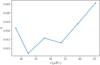 |
Fig. 24. Evolution of q throughout the binned spectrum presented in Fig. 23. |
| In the text | |
|
Fig. A.1. Evolution of the phase function with the frequency over the large speration. The phase function for different pressure radial orders is represented in blue. The straight line represents the identity function f(x) = x. Its intersections with the phase function are the solutions, in red. The grey square domains represent regions of constant np values. The vertical dashed lines are the positions of pure g-modes. The mixed-mode parameters used are q = 0.2 and ΔνΔπ1 = 200 |
| In the text | |
|
Fig. A.2. Second frequency difference δν2 as a function of the normalised period of mixed modes (dots). The red and blue colours are for q = 0.1 and q = 0.4, respectively. It is plotted for a typical value of ΔνΔπ1 = 200. The corresponding dashed curves show the evolution of 𝒩′. |
| In the text | |
Current usage metrics show cumulative count of Article Views (full-text article views including HTML views, PDF and ePub downloads, according to the available data) and Abstracts Views on Vision4Press platform.
Data correspond to usage on the plateform after 2015. The current usage metrics is available 48-96 hours after online publication and is updated daily on week days.
Initial download of the metrics may take a while.