| Issue |
A&A
Volume 642, October 2020
|
|
|---|---|---|
| Article Number | A226 | |
| Number of page(s) | 17 | |
| Section | Stellar structure and evolution | |
| DOI | https://doi.org/10.1051/0004-6361/202038834 | |
| Published online | 23 October 2020 | |
On attempting to automate the identification of mixed dipole modes for subgiant stars
Université Paris-Saclay, Institut d’Astrophysique Spatiale, UMR 8617, CNRS, Bâtiment 121, 91405 Orsay Cedex, France
e-mail: This email address is being protected from spambots. You need JavaScript enabled to view it.
Received:
3
July
2020
Accepted:
24
August
2020
Abstract
Context. The existence of mixed modes in stars is a marker of stellar evolution. Their detection serves for a better determination of stellar age.
Aims. The goal of this paper is to identify the dipole modes in an automatic manner without human intervention.
Methods. I used the power spectra obtained by the Kepler mission for the application of the method. I computed asymptotic dipole mode frequencies as a function of the coupling factor and dipole period spacing, as well as other parameters. For each star, I collapsed the power in an echelle diagramme aligned onto the monopole and dipole mixed modes. The power at the null frequency was used as a figure of merit. Using a genetic algorithm, I then optimised the figure of merit by adjusting the location of the dipole frequencies in the power spectrum. Using published frequencies, I compared the asymptotic dipole mode frequencies with published frequencies. I also used published frequencies to derive the coupling factor and dipole period spacing using a non-linear least squares fit. I used Monte-Carlo simulations of the non-linear least square fit to derive error bars for each parameter.
Results. From the 44 subgiants studied, the automatic identification allows one to retrieve within 3 μHz, at least 80% of the modes for 32 stars, and within 6 μHz, at least 90% of the modes for 37 stars. The optimised and fitted gravity-mode period spacing and coupling factor are in agreement with previous measurements. Random errors for the mixed-mode parameters deduced from the Monte-Carlo simulation are about 30−50 times smaller than previously determined errors, which are in fact systematic errors.
Conclusions. The period spacing and coupling factors of mixed modes in subgiants are confirmed. The current automated procedure will need to be improved upon using a more accurate asymptotic model and/or proper statistical tests.
Key words: asteroseismology / methods: data analysis / stars: interiors
© T. Appourchaux et al. 2020
 Open Access article, published by EDP Sciences, under the terms of the Creative Commons Attribution License (https://creativecommons.org/licenses/by/4.0), which permits unrestricted use, distribution, and reproduction in any medium, provided the original work is properly cited.
1. Introduction
The internal structure of stars has been derived with great detail with the advent of the space missions CoRoT and Kepler (Michel et al. 2008; Chaplin et al. 2010). The detection of pressure modes and mixed modes in red giants has provided a wealth of information about the internal structure of these stars (Mosser et al. 2014; Bedding et al. 2011) and their internal dynamics (Mosser et al. 2012a). Subgiant stars bridge the gap between the evolved red giants and the Main Sequence (MS) stars. Subgiant stars, being closer to MS stars, can help to infer information about the evolution of their interior and dynamics. For subgiant stars, Deheuvels et al. (2014) also measured their core rotation using these mixed modes. The properties of these mixed modes are such that they are easily detectable because they propagate like pressure modes until the surface of the star and they are excited by turbulent convection just as the pressure modes (Goldreich & Keeley 1977; Houdek et al. 1999; Dupret et al. 2009); however, these modes also propagate like gravity modes in the stellar core (Unno et al. 1989). Given these properties, these modes have also been searched for in the Sun with no positive results (Appourchaux et al. 2010).
The detection of these mixed modes in subgiant stars also provides an important marker of the age of these stars. The subgiants evolve away from the MS by burning hydrogen in shells after exhaustion on the hydrogen in the core. The time it takes for these stars to transition from the core exhaustion to the helium burning phase is called the first giant branch (Vassiliadis & Wood 1993). The time spent on this branch lasts about 15% to 30% of the time spent on the MS (Vassiliadis & Wood 1993). In addition, due to the presence of a helium core, there is a large increase in the Brunt-Vaïsala frequency, which makes the existence of a propagation zone for gravity modes possible (Dziembowski et al. 2001; Christensen-Dalsgaard 2004). It leads to the existence of the so-called mixed modes that have a pressure mode character in the outer stellar regions and a gravity mode character in the stellar core (Dziembowski et al. 2001; Christensen-Dalsgaard 2004). In addition, it is clear that since the change in the Brunt-Vaïsala frequency is so quick, the frequencies of the mixed modes change even faster because of their sensitivities to that frequency (Appourchaux et al. 2004). Therefore, the detection of mixed modes in subgiants is a powerful tool for getting a precise stellar age (Lebreton et al. 2014), even for getting a precise estimate of the mass (Deheuvels & Michel 2011).
A major challenge of the ESA PLATO mission is to derive stellar ages to better than 10% (Rauer et al. 2014) for the sample1 of stars that are brighter than mV = 11 magnitude and with an instrumental noise that is lower than 50 ppm h−1/2, provided with the 24 cameras (Marchiori et al. 2019; Moreno et al. 2019). The derivation of the stellar age is obtained by comparing theoretical mode frequencies to the observed mode frequencies (Lebreton et al. 2014). The number of stars in the P1 sample, for which an asteroseismic age with a precision can be derived to better than 10%, is larger than 8000. The measurement of the observed mode frequencies can be achieved using the following steps: detecting the stellar oscillation mode envelope, inferring the large separation of the modes (related to the diameter of the star), and tagging the degree of the modes and mode frequency fitting using either Maximum Likelihood Estimators or Markov chain Monte Carlo estimators. All of these steps can be automated in order to fit a large number of stars (see Mosser & Appourchaux 2009; Hekker et al. 2010, and references therein). These automated methods can be easily applied to MS stars that have no mixed modes (Fletcher et al. 2011).
It was already identified by Appourchaux et al. (2004) that the identification of mixed modes for a large number of in subgiants could be a challenge. For red giants having mixed modes, Vrard et al. (2016) devised a technique to automatically derive the gravity mode period spacing, allowing for one to fit the mixed modes. Their technique can be applied to stars for which the large separation is smaller than 18 μHz, but they used a guess for the gravity mode period spacing derived from Mosser et al. (2014); their technique is then not entirely automated. For subgiant stars, Bedding (2012) devised a replicated echelle diagram, allowing one to visually identify dipole mixed modes. For subgiants stars with a large separation typically higher than 30 μHz (Mosser et al. 2014), an automated detection procedure has recently been devised by Corsaro et al. (2020) for power spectra that have the l = 1 mode ridge slightly distorted. For a more complicated case, the mixed mode frequencies of the subgiant stars of Appourchaux et al. (2012a) were all identified by hand. In the case of PLATO, the manual identification becomes impractical for the mere 3000 subgiants of the P1 sample of PLATO, therefore requiring an automated procedure for that aim.
The goal of this paper is to present a way to automatically provide a guess for the frequencies of dipole mixed modes in subgiants. The first section recalls how the frequencies of these modes can be derived from an asymptotic expression based on the work of Shibahashi (1979) and of Mosser et al. (2015). The second section explains how one can build a diagnostic of the location of the mixed mode frequencies in a power spectrum derived from the Fourier transform of a stellar light curve (or from stellar radial velocity). The third section details how the diagnostic can be optimised to find the main characteristics of the parameters describing the location of the frequencies of the dipole mixed modes. The next three sections provides the results for about 44 subgiants and a few early red giants using the optimisation procedure and the fitting of available frequencies. I finally discuss the scientific implications and conclude.
2. Asymptotic mixed dipole mode frequency
The approach for the derivation of the asymptotic mixed mode frequency is based on the work of Mosser et al. (2015). The methodology is repeated here for completeness. The frequencies of the mixed dipole modes is asymptotic because the frequencies of the pressure modes and the gravity modes are assumed to follow the asymptotic description of Tassoul (1980). By definition, a mixed mode has a dual character of being both a pressure mode and a gravity mode. The main equation describing the mixed mode character is related to the following continuity equation provided by Shibahashi (1979):
 (1)
(1)
where θp and θg are the phase function of a dipole mixed mode frequency νpg, with respect to the frequency of p modes and g modes, and q is the coupling factor.
For the pressure mode phase function, the phase function θp is given by:
 (2)
(2)
where νnp, 1 is the frequency of the closest dipole pressure mode and Δν(np) is the large separation at order np. I note that νnp, 1 is given asymptotically by:
 (3)
(3)
where νnp, 0 is the radial mode frequency and d01 is the relative small separation between l = 0 and l = 1. In Mosser et al. (2015), they assume that the frequencies of the radial modes νnp, 0 are given by:
 (4)
(4)
where np is the order of the mode, ϵp is the p-mode phase offset, and α is the parameter describing the parabolic departure of the frequency from the asymptotic behaviour, nmax is the radial order at νmax, and Δν is the large separation. As a consequence, the large separation varies with the order as follows:
 (5)
(5)
Here, we note that the formulation of the l = 1 mode frequencies with respect to the l = 0 mode frequencies allows one to compensate for the surface effect directly. Since this effect is of a similar order for both, it is partly masked or even fully compensated for by the parabolic term in α.
For the gravity mode phase function, the phase function θg is given by:
 (6)
(6)
where νng, 1 is the frequency of the closest dipole gravity mode, ng is the order of the mode, and P1 is the period spacing of the dipole gravity mode. The frequency of the dipole gravity mode is given by:
 (7)
(7)
where ng is the g mode order (here it is positive) and ϵg is the g-mode phase offset. We note that P1 is related to P0 ( ).
).
For the asymptotic mixed mode frequencies, the frequencies νpg of the dipole mixed modes are then implicitly provided by solving the following equation:
 (8)
(8)
When there is no coupling q = 0, there are not any mixed modes νpg = νnp, 1. In practice, the steps involved in solving Eq. (8) is as follows:
-
Set Δν, ϵp, and α to the l = 0 mode frequencies (Eq. (4)).
-
Set d01 in order to get the l = 1 mode frequencies (Eq. (3)).
-
Set P1 and ϵg (Eq. (7)).
-
Set coupling factor q.
-
Compute phases using Eqs. (2) and (6). Set mixed mode frequency νng, 1 as a running frequency ν with a resolution of 1 nHz.
-
Compute the difference of the phase tangent as: δ(ν) = tanθp − qtanθg (Eq. (8)).
-
Compute the sign of δ. Since the derivative of δ(ν) wrt to ν is always positive, δ(ν) is an increasing function of ν, then the only transition through zero is when δ changes sign from negative to positive. When this occurs, it means that it has crossed the zero line, that is, we have a solution for a mixed-mode frequency.
-
The final detection of the location of the mixed-mode frequency is carried out by computing the first difference of the sign of δ. When there is a crossing from negative to positive, the first difference is then 2 (+1−(−1)).
This pseudo code can easily be implemented in any language.
3. Collapsing of mixed-mode peak power
The identification of dipole mixed modes in subgiant stars rely on a visual assessment of the location of the mixed modes. As mentioned earlier, the use of a replicated echelle diagram (Bedding 2012) or just plain experience of a regular or irregular echelle diagram is sufficient for most applications, that is, for tens of stars. For the PLATO mission, I had to devise an automated procedure that would make the identification more immune to human intervention. The novelty of the method developed in this section lies in the use of all the information available in the power spectrum for the monopole and dipole modes coupled with the asymptotic description introduced in the previous section. The information used allows one to derive a figure of merit that is related to the location of the dipole mode frequencies in the power spectrum.
The idea behind the derivation of the guess frequencies for the dipole mixed modes is based on the visualisation of the échelle diagram (Grec 1981) applied to a power spectrum of stellar time series. If one co-adds the power along each segment line of the échelle, one obtains the so-called collapsed power. An example of a collapsed power is shown in Fig. 1 where one can see two main doublets: one doublet for the l = 0−2 modes located at 0 μHz and one doublet for the l = 1−3 modes located at +63 μHz. The other patches of power located at −35 μHz and +18 μHz seen in Fig. 1 are due to the l = 4 modes and the l = 5 modes, respectively. Figure 1 was computed using data from the Luminosity Oscillations Imager (LOI) seeing the Sun as a star (Appourchaux et al. 1997). The additional sensitivity to the higher degree modes are due to the LOI pixels resolving the surface of the Sun (ibidem).
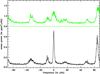 |
Fig. 1. Superposed power for the LOI data: power averaged over 15 modes centred on the l = 0 modes: (top, green) for a fixed large separation of 136 μHz; (bottom, black) for an optimised large separation of 134.7 μHz linearly dependent on frequency. The original power spectrum, smoothed to ten bins, is taken from one year of data of the Luminosity Oscillations Imager seeing the Sun as a star (Appourchaux et al. 1997). |
Figure 2 shows the collapsed power for a KIC 11137075, a star with l = 1 mixed modes already analysed by Tian et al. (2015). It is obvious that the power of the l = 1 mixed modes is not concentrated at all, compared to the l = 0−2 mode pairs. The idea was then to compute l = 1 mixed mode frequencies, resulting from solving Eq. (8), and to collapse the power around these frequencies. The power was then extracted around an l = 1 mixed frequency using a window of the size of the large separation (±Δν/2), then the power was summed up over all l = 1 mixed modes found from solving Eq. (8). Here, the total power was not averaged over the number of mixed modes because the division would prevent from having a large total power when more mixed modes correspond to the real peak of power. In addition, since I am interested in the location of the dipole mode frequencies, I compensated for the intrinsic fall out of mode power away from νmax by dividing the original power spectrum by the inverse of a Gaussian mode envelope whose full width at half maximum is 2/3 of the full mode frequency range defined as [νlow,νhigh]. This compensation permits one to give a lower weight to the modes close to νmax, and a higher weight to the modes on the edge of the p-mode range.
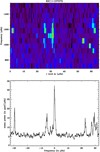 |
Fig. 2. Top: echelle diagram for KIC 11137075 with a large separation of 65 μHz. Bottom: superposed power for KIC 11137075 star: power averaged over eight modes centred on the l = 0 modes. The original power spectrum, smoothed to ten bins, is taken from 6 months of Kepler data. |
4. Optimisation of collapsed power
The computation of the collapsed power was performed as explained in the previous section. Then I needed a way to optimise the location of the l = 0 mode frequencies and of the l = 1 mode frequencies. The next idea was to compute the mean collapsed power within 1 μHz of the centre located at 0 μHz. I used this mean power as a figure of merit, which was then maximised. The procedure was done in the following steps:
-
Get a stellar power spectrum, smooth it over ten bins.
-
Select a frequency range for the p-mode power as [νlow,νhigh].
-
Divide the power spectrum by a proxy of the Gaussian envelope.
-
Optimise for the l = 0 mode frequencies:
-
(a)
Set a starting value for Δν, ϵp, and α for the l = 0 mode frequencies (Eq. (4)).
-
(b)
Compute the collapsed power and determine the figure of merit for l = 0.
-
(c)
Optimise (Δν, ϵp, and α) in order to obtain the highest figure of merit for l = 0.
-
(a)
-
Optimise for the l = 1 mode frequencies:
-
(a)
Use the previously determined (Δν, ϵp, and α) as fixed value.
-
(b)
Set d01 to determine the l = 1 p-mode frequencies (Eq. (3)).
-
(c)
Set starting values for P1 and ϵg in order to obtain the l = 1 g-mode frequencies (Eq. (7)).
-
(d)
Set a starting value for q.
-
(e)
Get l = 1 mixed mode frequencies from solving Eq. ((8)).
-
(f)
Compute collapsed power and get the figure of merit for l = 1.
-
(g)
Optimise (d01, P1, ϵg, q) to determine the highest figure of merit for l = 1.
-
(a)
The maximisation of the l = 0 figure of merit (step 2c) was performed using a regular steepest-descent method since it is clear that there is only one minima that is very local and very close to the guess value of Δν, ϵp, and α. The maximisation of the l = 1 figure of merit (step 5g) is a lot more complicated. Regular algorithms based on the steepest descent fail because of the many local extrema. An algorithm that is able to search for the extremum of local extrema must be used in order to find a proper solution. Different algorithms were attempted, such as the following ones: random search, Gaussian process prediction, genetic algorithm.
The random search is a brute force method, which consists in performing a 1 million evaluation of the l = 1 figure of merit taken from the four parameters taken at random in a hypercube for the four parameters that are to be searched. This algorithm was used for a similar problem involving solar g-mode detection (Appourchaux & Corbard 2019). The algorithm does find the global extremum, but it is very slow due to the large number of function evaluations.
Another approach tested was to use the Gaussian processes (GP) when evaluating and forecasting the figure of merit in the hypercube (see Frazier 2018, for a tutorial). An instructive application of GP can be found in Jones et al. (1998). The application of GP is most useful when the figure of merit that is to be computed takes a large amount of time in the hyperspace. Instead of computing the figure of merit on a very fine grid of the hyperspace in order to find the extremum, the idea is to forecast, with a small number of calculations, the shape of the figure of merit in hyperspace, and from there to sample the next point in hyperspace in order to check the extremum of the forecasted figure of merit. Usually the sampling of the next point in hyperspace is done by computing another figure of merit called the Expected Improvement (EI). The EI function can be much faster than the original figure of merit to compute on a fine grid of the hyperspace. Although this is a promising approach, the transfer of the optimisation problem from the figure of merit to EI works on a small number of parameters (i.e. less than three), but it fails for four parameters because the EI has local maxima that are Dirac-like, which are then easily missed unless the computing grid is extremely fine. The original figure of merit already has a large variation and it does not vary slowly; in hyperspace, the EI is then similar to an empty space, with a small hypersphere that is sparsely distributed.
The most useful algorithm for the current problem is based on a genetic approach. The optimisation is based on the Shuffled Complex Evolution (SCE) algorithm, which mixes evolutionary and simplex algorithms (Duan et al. 1993). This algorithm allows one to search for the best maximum overall, and then search for the highest maximum locally. This algorithm was used by Thi et al. (2010) to fit the absorption profile observed in the infrared with the European Southern Observatory’s Very Large Telescope. The fit employs an Interactive Data Language (IDL) software, which can be found at Thi’s home page2, which I used for the optimisation of the figure of merit. Owing to the random characteristics of the genetic algorithm, I also chose to run the SCE in several steps as follows:
-
(1)
Perform optimisation ten times using the SCE with the following parameters: d01 = [ − 0.2, 0.1], ϵg = [0.2, 0.7], q = [0.,0.8], P1 = [100.,1000.].
-
(2)
Determine the minimum and maximum of the optimised P1 amongst the ten. Compute
 ,
,  .
. -
(3)
Carry out optimisation ten times using the SCE with the following parameters and the same range for: d01, ϵg, q,
![Mathematical equation: $ P_1=[P_1^{\rm mean}-1.1\Delta_{P1}, P_1^{\rm mean}+1.1\Delta_{P1}] $](/articles/aa/full_html/2020/10/aa38834-20/aa38834-20-eq12.gif) .
.
This is more efficient than running a million evaluations of the figure of merit since it results in about ten fewer evaluations in total. Table 1 gives the parameters resulting from the optimisation for each star.
Optimised parameters.
Figures 3−5 show the results of the optimisation for three typical cases. The (P1, q) maps show the difficulties involved in finding the maximum of the figure of merit. The typical cases are as follows:
-
For a period spacing that is larger than 200−300 s, a maximum is clearly located below 0.2 for q. Lower local maxima are present but they can clearly be excluded (Fig. 3).
-
For a q that is larger than 0.2, several local maxima are located along parallel ridges along q.
-
For P1 that is less than 200 s, there are several isolated local maxima.
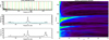 |
Fig. 3. Left, top: power spectrum as a function of frequency for KIC 6442183. The power spectrum is compensated for the p-mode envelope power. The vertical orange lines indicate the location of the l = 0 modes for which the power was set to zero. The vertical green lines indicate the location of the dipole mixed modes. The vertical red lines indicate the location of the gravity modes. Left, middle: superposed power as a function of the frequency for the dipole modes (l = 1); the horizontal cyan line indicates the level of noise. Left, bottom: superposed power as a function of frequency for the l = 0 modes. Right: map of the figure of merit for (P1, q) with all other parameters fixed. |
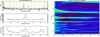 |
Fig. 4. Left, top: power spectrum as a function of the frequency for KIC 9512063. The power spectrum is compensated for the p-mode envelope power. The vertical orange lines indicate the location of the l = 0 modes for which the power was set to zero. The vertical green lines indicate the location of the dipole mixed modes. The vertical red lines indicate the location of the gravity modes. Left, middle: superposed power as a function of the frequency for the dipole modes (l = 1); the horizontal cyan line indicates the level of noise. Left, bottom: superposed power as a function of the frequency for the l = 0 modes. Right: map of the figure of merit for (P1, q) with all other parameters fixed. |
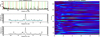 |
Fig. 5. Left, top: power spectrum as a function of frequency for KIC 12508433. The power spectrum is compensated for the p-mode envelope power. The vertical orange lines indicate the location of the l = 0 modes for which the power was set to zero. The vertical green lines indicate the location of the dipole mixed modes. The vertical red lines indicate the location of the gravity modes. Left, middle: superposed power as a function of the frequency for the dipole modes (l = 1); the horizontal cyan line indicates the level of noise. Left, bottom: superposed power as a function of the frequency for the l = 0 modes. Right: map of the figure of merit for (P1, q) with all other parameters fixed. |
The boundaries for these categories are by no means exact, but just rough indications. Some stars may fall in one category or the other, while still being outside of the defined boundaries. Even so, the three maps are typical of the various maps observed. From these maps, it is obvious that the optimisation is not a simple problem as many local minima may prevent one to find the global minimum (see Fig. 5).
5. Results from optimisation: Period spacing and coupling factor
I used two criteria that are useful to separate the red giants from the subgiants: the evolution criteria and the density of mixed modes. Mosser et al. (2014) provided a boundary for the evolution criteria that subgiants fulfill (Δν/36.5 μHz) (P1/126 s) > 1. The density of mixed modes is equivalent, to the first order, to the ratio of the gravity-mode order to the pressure mode-order (𝒩 ∼ ng/np); Mosser et al. (2012b) gave this density as  .
.
Figure 6 shows the comparison with the measurement made using the asymptotic relation as in Mosser et al. (2014), and using the same avoided crossing as in Li et al. (2020) for the period spacing. I note that the period spacing as derived from the asymptotic relation of Shibahashi (1979) cannot be directly compared with the formulation used by Deheuvels & Michel (2011) based on the avoided crossing for harmonic oscillators. For example, Benomar et al. (2013) and Li et al. (2020) provide several examples of echelle diagrams, indicating the location of the frequency of the gravity modes (γ modes) using the formalism of Deheuvels & Michel (2011). It is clear that the resulting frequencies of the mixed modes are greatly affected close to the frequency location of the gravity γ modes, that is, the mixed modes are further away than the regular l = 1 ridge. On the other hand, the mixed modes are closer to the original ridge in between the gravity γ mode frequencies. In the formalism of Shibahashi (1979), the situation is the opposite. That is to say, close to a gravity mode, the mixed mode frequency is close to the original dipole mode frequency since θg ∼ 0, then θp ∼ 0; but when θg ∼ π/2, then θp ∼ π/2, which means that the mixed mode frequency can be anywhere within a Δν. In the formalism of Shibahashi (1979), the gravity modes have a g-mode phase offset of 1/2 compared to the gravity γ mode of Benomar et al. (2013).
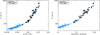 |
Fig. 6. Left: period spacing of the dipole modes as a function of the number of g modes. Right: period spacing of the dipole modes as a function of the evolution criteria. Black discs: from the optimisation procedure; blue crosses: from Mosser et al. (2014); orange crosses: from Li et al. (2020). |
Figure 7 shows the comparison with the measurement made by Mosser et al. (2017) for the coupling factor (supplemented by data shown in Mosser et al. 2017 but not published; Mosser, 2020, priv. comm.). The comparison shows very good agreement with the work of Mosser et al. (2014, 2017). The period spacings from the optimisation are also in agreement with the results of Deheuvels et al. (2014). The increase in the coupling factor for subgiant stars is due to a very thin zone where mixed modes are evanescent (Pinçon et al. 2020). This is the strong coupling assumption that leads to high transmission between the gravity mode cavity and that of the pressure mode cavity (Takata 2016).
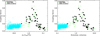 |
Fig. 7. Left: coupling factor as a function of the number of g modes. Right: coupling factor as a function of the evolution criteria. Black discs: from the optimisation procedure; blue crosses: from Mosser et al. (2017); green crosses: from Mosser (2020, priv. comm.) for Δν > 30 μHz but unpublished in Mosser et al. (2017). |
It is also quite clear that there is a simple relation between the evolution criteria and the density of mixed modes. Since νmax depends on the large separation, it can be shown that the density of mixed modes is inversely proportional to the power of the evolution criteria; depending on the state of evolution, the exponent factor varies from −1 (for subgiants) to −1.5 (for red giants). A better relation can be derived, but the end result is that the evolution criteria, as devised by Mosser et al. (2014), is sufficient for understanding the complexity of the mixed-mode pattern.
6. Results from optimisation: d01 and ϵp
Figure 8 shows the relative small separation obtained from the optimisation compared to previous measurements obtained by Benomar et al. (2013). The results are comparable with the relative small separation provided by Stello et al. (2012) for a 1 M⊙ star. The small separation d01 is much less powerful in terms of the asteroseismic diagnostic compared to the small separation d02 that can provide an estimate or proxy of stellar ages (Lebreton & Montalbán 2009; Appourchaux et al. 2015).
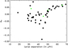 |
Fig. 8. Relative small separation d01 as a function of the large separation. Black discs: from the optimisation procedure; green discs: from Benomar et al. (2013). |
Figure 9 shows ϵp as a function of the effective temperature compared to a theoretical model from Li et al. (2020). This (ϵp, Teff) diagram can be used as a diagnostic to identify the l = 0−2 modes versus the l = 1 modes for stars with a high effective temperature for which the mode linewidth is larger than the small separation δ02 (White et al. 2011). In the case of subgiant stars, the identification is eased because of the presence of mixed modes. The dependence of ϵp with a high effective temperature for the subgiant stars is similar to that of White et al. (2011).
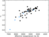 |
Fig. 9. ϵp as a function of the effective temperature. Black discs: from the optimisation procedure; blue discs: from the theoretical model of zero age MS stars given by Li et al. (2020). |
7. Results: Asymptotic frequencies versus fitted frequencies
For 35 stars out of the 44 stars, we fitted the frequencies available from Campante et al. (2011), Appourchaux et al. (2012b), Deheuvels et al. (2014), Tian et al. (2015), and Li et al. (2020). We used those frequencies for comparison purposes with the location of the asymptotic dipole frequencies that could have been used as a guess. For the remaining nine stars, I visually checked whether or not a mode was present close to the asymptotic dipole frequency. Table 1 provides the percentage of frequencies (fitted or visual) that are within 3 μHz of the asymptotic frequencies. The automatic identification allows one to retrieve, within 3 μHz, at least 80% of the modes for 32 stars and, within 6 μHz, at least 90% of the modes for 37 stars. Figure 10 shows the best and worst matching for stars with fitted frequencies. Figure 11 shows the best and worst matching for stars with visual frequencies. Figure A.1 give the comparison for all of the other stars with fitted frequencies.
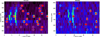 |
Fig. 10. Echelle diagram of the amplitude spectra with: dipole frequencies fitted on the power spectra (red circles); l = 0 frequencies from the optimisation (orange diamonds); asymptotic dipole frequencies from the optimisation (white diamonds); and dipole frequencies from fitting the asymptotic model to the fitted frequencies (red diamonds). Left: for a case where 100% of the asymptotic frequencies match the fitted frequencies. Right: for a case where 55% of the asymptotic frequencies match the fitted frequencies. |
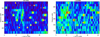 |
Fig. 11. Echelle diagram of the amplitude spectra with visual frequencies for the dipole modes (orange circles) and the asymptotic dipole frequencies from the optimisation (white and black crosses). Left: for a case where 100% of the asymptotic frequencies match the visual frequencies. Right: for a case where 80% of the asymptotic frequencies match the visual frequencies. |
It is known that the asymptotic approximation is not applicable for mixed modes in subgiants (Deheuvels et al. 2014). This is mainly due to the dipole mode frequency being of the same order of magnitude as that of the Brunt-Vaïsala frequency. In addition, Ong & Basu (2020) mention that the asymptotic approximation fails for low ng and high np, which is the case when the density of mixed mode 𝒩 is less than 1. For most of the stars, the agreement is quite remarkable (left of Fig. 10). Nevertheless a success rate of 80% is not satisfactory for an automatic guess determination. It means, for instance, that out of the 3000 subgiants from the P1 sample of PLATO, 900 stars have between 50% and 80% of their dipole mode frequencies properly fitted.
8. Results from least square fit: Period spacing, coupling factor, and d01
The optimisation procedure does not provide direct access to the error bars for each parameter. I could have derived the error bars from a Monte-Carlo simulation of the optimisation process, but this would have taken a vary long time. In addition, it would not have been particularly pertinent because the original goal of the optimisation was to obtain guess frequencies for the proper extraction of the dipole mode frequencies.
Therefore, I chose to directly fit the asymptotic frequencies to the fitted frequencies. In so doing, it is feasible to perform a Monte-Carlo simulation of the fitting by using the error bars provided for the fitted frequencies by several authors. As outline previously, the asymptotic model is far from perfect. For several stars, the deviation of the asymptotic frequencies to the fitted frequencies can be very large, amounting to more than 1000σ. In other words, the fit is plagued with systematic errors due to the model itself. Therefore, in order to fit the model using the fitted frequencies, I chose to minimise the unweighted least square fit. To compute error bars for the four parameters defining the location of the dipole mixed modes, I ran 100 Monte-Carlo simulations of the least square fitting using the fitted frequencies and their error bars as randomised input. For the least square fit, I also used the SCE algorithms with the following ranges: d01 = [ − 0.2, 0.2], ϵg = [0.,2.0], q = [0.,1.0], P1 = [0.6Poptim, 1.4Poptim]; where Poptim is the period spacing from the optimisation procedure. In contrast, Buysschaert et al. (2016) also used a non-linear least square fit, while also using a grid search for three parameters (ϵg, q, and P1). Table 2 provides the results of the fit with their error bars. I note that only the dipole mode frequencies were fitted in the process; the parameters defining the l = 0 mode frequencies were assumed to be the same as for the optimisation.
Fitted parameters.
Figure 12 provides the result of the fit compared to the optimisation for the coupling factor and the period spacing, which shows a good agreement between the two determinations. Figure 13 provides the errors from the Monte-Carlo simulation for the coupling factor and the period spacing. In this figure, I added the error bars derived by Mosser et al. (2014), which are rather large compared to the error bars derived from the Monte-Carlo simulation. A simple explanation for these large error bars is that the many solutions providing the period spacing can be mistreated as an error while it is a simple systematic error. Multiple solutions for the period spacing arise when, for a given g-mode frequency at ng, P1 can be expressed such that:
 (9)
(9)
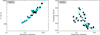 |
Fig. 12. Left: period spacing of the dipole modes as a function of the number of g modes. Right: period spacing of the dipole modes as a function of the evolution criteria. Black discs: from the optimisation procedure; cyan discs: from the fit of the frequencies. |
leading to
 (10)
(10)
I can replace (ng + 1 + ϵg) with Pmax/P1, where Pmax is the period corresponding to νmax. Then I have:
 (11)
(11)
This is a rather crude approximation since the next g-mode frequency (ng + 1) should have also been taken into account. It just gives a simple explanation for multiple solutions. The same equation as Eq. (11) was given by Vrard et al. (2016), but with a different meaning. As a matter of fact, this equation does not provide an estimate for an error, as stated by Vrard et al. (2016), but a separation between multiple solutions, or pseudo-periodic solutions. Figures 3–5 give good examples of the pseudo-periodic solutions that are roughly separated according to Eq. (11). As shown by Fig. 13, the error derived by Mosser et al. (2014) are very close to the systematic error provided by Eq. (11). This explains why my error bars for the period spacing are about 30−50 times smaller than these systematics errors.
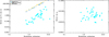 |
Fig. 13. Left: error on the period spacing of the dipole modes as a function of the number of g modes. Right: error on the coupling factor of the dipole modes as a function of the evolution criteria. Black discs: from the optimisation procedure; cyan discs: from the fit of the frequencies; blue crosses: error from Mosser et al. (2014); orange crosses: systematics from Eq. (11). |
Figure 14 shows the relative small separation obtained from the frequency fit compared to the optimisation and to previous measurements obtained by Benomar et al. (2013). The results with the fit are not very different from the optimisation procedure.
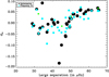 |
Fig. 14. Relative small separation d01 as a function of the large separation. Black discs: from the optimisation procedure; cyan discs: from the fit of the frequencies; green discs: from Benomar et al. (2013). |
9. Discussion
Several alleys for improvement of the method are envisaged that use a combination of an improved asymptotic description together with a detection scheme similar to that of Corsaro et al. (2020). The improvement should lead to an automatic identifying guess with a success rate that is better than 99%. The application of the optimisation procedure for the l = 2 and l = 3 mixed modes can be envisaged in a very similar fashion.
The current computation of the figure of merit does not take into account the variation in mode height due to the mode inertia, as was observed by Benomar et al. (2014) for a couple of subgiant stars. The extension of the method to red giants would require taking the variation of the mode height with the dipole mode frequency into account. Dupret et al. (2009) showed that many dipole mixed modes are strongly attenuated, and they would not contribute to any power in the figure of merit. Benomar et al. (2014) and Mosser et al. (2015) provide an asymptotic expression for the mixed mode inertia that can be used for both subgiant and red giants. Last but not least, the rotational splitting is not included in the current model, but it would be necessary as the rotation in red giants can be similar to the mixed mode spacing in Mosser et al. (2015).
10. Conclusion
In this paper, I present a new way of deriving the coupling factors and period spacing of dipole mixed modes. The results obtained are in agreement with previous measurements made by Mosser et al. (2014, 2017). I also obtained error bars on the parameters defining the dipole mixed modes using Monte-Carlo simulations. The automated procedure is far from being perfect as it can provide, for 32 stars out of 44 stars, 80% of the dipole mode frequencies to within ±3 μHz of the dipole peak power. The improvements of the method for subgiant stars and the extension to red giant stars are discussed.
Known as the P1 sample.
Acknowledgments
Many thanks to my family for the long standing support during the exploration, questioning, computing, and writing phase of this paper. Thanks also to the confinement, I had ample time to finish this cursed paper that merely took 18 months to complete. Thanks to the Kepler gang for allowing us to play with such wonderful data. This paper benefitted from discussions with Othman Benomar, Patrick Gaulme, Benoit Mosser, Charly Pinçon, and Mathieu Vrard. Several of my forefathers and colleagues contributed in absentia to this paper: Jacques-Emile Blamont, Pierre Connes, Vicente Domingo, Claus Fröhlich and David M. Rust.
References
- Appourchaux, T., & Corbard, T. 2019, A&A, 624, A106 [NASA ADS] [CrossRef] [EDP Sciences] [Google Scholar]
- Appourchaux, T., Andersen, B. N., Fröhlich, C., et al. 1997, Sol. Phys., 170, 27 [NASA ADS] [CrossRef] [Google Scholar]
- Appourchaux, T., Moreira, O., Berthomieu, G., & Toutain, T. 2004, in Stellar Structure and Habitable Planet Finding, eds. F. Favata, S. Aigrain, & A. Wilson, ESA SP, 538, 109 [Google Scholar]
- Appourchaux, T., Belkacem, K., Broomhall, A.-M., et al. 2010, A&ARv, 18, 197 [NASA ADS] [CrossRef] [Google Scholar]
- Appourchaux, T., Benomar, O., Gruberbauer, M., et al. 2012a, A&A, 537, A134 [NASA ADS] [CrossRef] [EDP Sciences] [Google Scholar]
- Appourchaux, T., Chaplin, W. J., García, R. A., et al. 2012b, A&A, 543, A54 [NASA ADS] [CrossRef] [EDP Sciences] [Google Scholar]
- Appourchaux, T., Antia, H. M., Ball, W., et al. 2015, A&A, 582, A25 [NASA ADS] [CrossRef] [EDP Sciences] [Google Scholar]
- Bedding, T. R. 2012, in Progress in Solar/Stellar Physics with Helio- and Asteroseismology, eds. H. Shibahashi, M. Takata, & A. E. Lynas-Gray, ASP Conf. Ser., 462, 195 [Google Scholar]
- Bedding, T. R., Mosser, B., Huber, D., et al. 2011, Nature, 471, 608 [NASA ADS] [CrossRef] [PubMed] [Google Scholar]
- Benomar, O., Bedding, T. R., Mosser, B., et al. 2013, ApJ, 767, 158 [NASA ADS] [CrossRef] [Google Scholar]
- Benomar, O., Belkacem, K., Bedding, T. R., et al. 2014, ApJ, 781, L29 [NASA ADS] [CrossRef] [PubMed] [Google Scholar]
- Buysschaert, B., Beck, P. G., Corsaro, E., et al. 2016, A&A, 588, A82 [NASA ADS] [CrossRef] [EDP Sciences] [Google Scholar]
- Campante, T. L., Handberg, R., Mathur, S., et al. 2011, A&A, 534, A6 [NASA ADS] [CrossRef] [EDP Sciences] [Google Scholar]
- Chaplin, W. J., Appourchaux, T., Elsworth, Y., et al. 2010, ApJ, 713, L169 [NASA ADS] [CrossRef] [Google Scholar]
- Christensen-Dalsgaard, J. 2004, Sol. Phys., 220, 137 [Google Scholar]
- Corsaro, E., McKeever, J. M., & Kuszlewicz, J. S. 2020, A&A, 640, A130 [CrossRef] [EDP Sciences] [Google Scholar]
- Deheuvels, S., & Michel, E. 2011, A&A, 535, A91 [NASA ADS] [CrossRef] [EDP Sciences] [Google Scholar]
- Deheuvels, S., Doğan, G., Goupil, M. J., et al. 2014, A&A, 564, A27 [NASA ADS] [CrossRef] [EDP Sciences] [Google Scholar]
- Duan, Q. Y., Gupta, V. K., & Sorooshian, S. 1993, J. Optim. Theor. Appl., 76, 501 [CrossRef] [Google Scholar]
- Dupret, M. A., Belkacem, K., Samadi, R., et al. 2009, A&A, 506, 57 [NASA ADS] [CrossRef] [EDP Sciences] [Google Scholar]
- Dziembowski, W. A., Gough, D. O., Houdek, G., & Sienkiewicz, R. 2001, MNRAS, 328, 601 [NASA ADS] [CrossRef] [Google Scholar]
- Fletcher, S. T., Broomhall, A. M., Chaplin, W. J., et al. 2011, MNRAS, 413, 359 [NASA ADS] [CrossRef] [Google Scholar]
- Frazier, P. I. 2018, ArXiv e-prints [arXiv:1807.02811] [Google Scholar]
- Goldreich, P., & Keeley, D. A. 1977, ApJ, 212, 243 [NASA ADS] [CrossRef] [Google Scholar]
- Grec, G. 1981, PhD Thesis, Université de Nice [Google Scholar]
- Hekker, S., Broomhall, A. M., Chaplin, W. J., et al. 2010, MNRAS, 402, 2049 [NASA ADS] [CrossRef] [Google Scholar]
- Houdek, G., Balmforth, N. J., Christensen-Dalsgaard, J., & Gough, D. O. 1999, A&A, 351, 582 [NASA ADS] [Google Scholar]
- Jones, D. R., Schonlau, M., & Welch, W. J. 1998, J. Glob. Optim., 13, 455 [CrossRef] [MathSciNet] [Google Scholar]
- Lebreton, Y., & Montalbán, J. 2009, in The Ages of Stars, eds. E. E. Mamajek, D. R. Soderblom, & R. F. G. Wyse, IAU Symp., 258, 419 [Google Scholar]
- Lebreton, Y., Goupil, M. J., & Montalbán, J. 2014, EAS Pub. Ser., 65, 177 [CrossRef] [Google Scholar]
- Li, Y., Bedding, T. R., Li, T., et al. 2020, MNRAS, 495, 2363 [CrossRef] [Google Scholar]
- Marchiori, V., Samadi, R., Fialho, F., et al. 2019, A&A, 627, A71 [CrossRef] [EDP Sciences] [Google Scholar]
- Michel, E., Baglin, A., Auvergne, M., et al. 2008, Science, 322, 558 [NASA ADS] [CrossRef] [PubMed] [Google Scholar]
- Moreno, J., Vielba, E., Manjón,, A., et al. 2019, in SPIE Conf. Ser., Proc. SPIE, 11180, 111803N [Google Scholar]
- Mosser, B., & Appourchaux, T. 2009, A&A, 508, 877 [NASA ADS] [CrossRef] [EDP Sciences] [Google Scholar]
- Mosser, B., Goupil, M. J., Belkacem, K., et al. 2012a, A&A, 548, A10 [NASA ADS] [CrossRef] [EDP Sciences] [Google Scholar]
- Mosser, B., Goupil, M. J., Belkacem, K., et al. 2012b, A&A, 540, A143 [NASA ADS] [CrossRef] [EDP Sciences] [Google Scholar]
- Mosser, B., Benomar, O., Belkacem, K., et al. 2014, A&A, 572, L5 [NASA ADS] [CrossRef] [EDP Sciences] [PubMed] [Google Scholar]
- Mosser, B., Vrard, M., Belkacem, K., Deheuvels, S., & Goupil, M. J. 2015, A&A, 584, A50 [NASA ADS] [CrossRef] [EDP Sciences] [Google Scholar]
- Mosser, B., Pinçon, C., Belkacem, K., Takata, M., & Vrard, M. 2017, A&A, 600, A1 [NASA ADS] [CrossRef] [EDP Sciences] [Google Scholar]
- Ong, J. M. J., & Basu, S. 2020, ApJ, 898, 127 [CrossRef] [Google Scholar]
- Pinçon, C., Goupil, M. J., & Belkacem, K. 2020, A&A, 634, A68 [CrossRef] [EDP Sciences] [Google Scholar]
- Rauer, H., Catala, C., Aerts, C., et al. 2014, Exp. Astron., 38, 249 [NASA ADS] [CrossRef] [Google Scholar]
- Shibahashi, H. 1979, PASJ, 31, 87 [NASA ADS] [Google Scholar]
- Stello, D. 2012, in Progress in Solar/Stellar Physics with Helio- and Asteroseismology, eds. H. Shibahashi, M. Takata, & A. E. Lynas-Gray, ASP Conf. Ser., 462, 200 [Google Scholar]
- Takata, M. 2016, PASJ, 68, 91 [NASA ADS] [CrossRef] [Google Scholar]
- Tassoul, M. 1980, ApJS, 43, 469 [NASA ADS] [CrossRef] [Google Scholar]
- Thi, W. F., van Dishoeck, E. F., Pontoppidan, K. M., & Dartois, E. 2010, MNRAS, 406, 1409 [Google Scholar]
- Tian, Z., Bi, S., Bedding, T. R., & Yang, W. 2015, A&A, 580, A44 [CrossRef] [EDP Sciences] [Google Scholar]
- Unno, W., Osaki, Y., Ando, H., Saio, H., & Shibahashi, H. 1989, Nonradial Oscillations of Stars, 2nd edn. (Tokyo: University of Tokyo Press) [Google Scholar]
- Vassiliadis, E., & Wood, P. R. 1993, ApJ, 413, 641 [NASA ADS] [CrossRef] [Google Scholar]
- Vrard, M., Mosser, B., & Samadi, R. 2016, A&A, 588, A87 [NASA ADS] [CrossRef] [EDP Sciences] [Google Scholar]
- White, T. R., Bedding, T. R., Stello, D., et al. 2011, ApJ, 743, 161 [NASA ADS] [CrossRef] [Google Scholar]
Appendix A: Additional figures
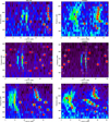 |
Fig. A.1. Echelle diagram for six stars. Frequencies fitted on the power spectra (red circles). Frequencies from the optimisation: l = 0 (orange diamonds), l = 1 (white diamonds). Frequencies from fitting the asymptotic model on the fitted frequencies (red diamonds). |
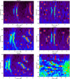 |
Fig. A.1. continued. |
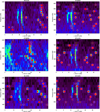 |
Fig. A.1. continued. |
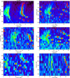 |
Fig. A.1. continued. |
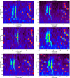 |
Fig. A.1. continued. |
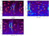 |
Fig. A.1. continued. |
All Tables
All Figures
|
Fig. 1. Superposed power for the LOI data: power averaged over 15 modes centred on the l = 0 modes: (top, green) for a fixed large separation of 136 μHz; (bottom, black) for an optimised large separation of 134.7 μHz linearly dependent on frequency. The original power spectrum, smoothed to ten bins, is taken from one year of data of the Luminosity Oscillations Imager seeing the Sun as a star (Appourchaux et al. 1997). |
| In the text | |
|
Fig. 2. Top: echelle diagram for KIC 11137075 with a large separation of 65 μHz. Bottom: superposed power for KIC 11137075 star: power averaged over eight modes centred on the l = 0 modes. The original power spectrum, smoothed to ten bins, is taken from 6 months of Kepler data. |
| In the text | |
|
Fig. 3. Left, top: power spectrum as a function of frequency for KIC 6442183. The power spectrum is compensated for the p-mode envelope power. The vertical orange lines indicate the location of the l = 0 modes for which the power was set to zero. The vertical green lines indicate the location of the dipole mixed modes. The vertical red lines indicate the location of the gravity modes. Left, middle: superposed power as a function of the frequency for the dipole modes (l = 1); the horizontal cyan line indicates the level of noise. Left, bottom: superposed power as a function of frequency for the l = 0 modes. Right: map of the figure of merit for (P1, q) with all other parameters fixed. |
| In the text | |
|
Fig. 4. Left, top: power spectrum as a function of the frequency for KIC 9512063. The power spectrum is compensated for the p-mode envelope power. The vertical orange lines indicate the location of the l = 0 modes for which the power was set to zero. The vertical green lines indicate the location of the dipole mixed modes. The vertical red lines indicate the location of the gravity modes. Left, middle: superposed power as a function of the frequency for the dipole modes (l = 1); the horizontal cyan line indicates the level of noise. Left, bottom: superposed power as a function of the frequency for the l = 0 modes. Right: map of the figure of merit for (P1, q) with all other parameters fixed. |
| In the text | |
|
Fig. 5. Left, top: power spectrum as a function of frequency for KIC 12508433. The power spectrum is compensated for the p-mode envelope power. The vertical orange lines indicate the location of the l = 0 modes for which the power was set to zero. The vertical green lines indicate the location of the dipole mixed modes. The vertical red lines indicate the location of the gravity modes. Left, middle: superposed power as a function of the frequency for the dipole modes (l = 1); the horizontal cyan line indicates the level of noise. Left, bottom: superposed power as a function of the frequency for the l = 0 modes. Right: map of the figure of merit for (P1, q) with all other parameters fixed. |
| In the text | |
|
Fig. 6. Left: period spacing of the dipole modes as a function of the number of g modes. Right: period spacing of the dipole modes as a function of the evolution criteria. Black discs: from the optimisation procedure; blue crosses: from Mosser et al. (2014); orange crosses: from Li et al. (2020). |
| In the text | |
|
Fig. 7. Left: coupling factor as a function of the number of g modes. Right: coupling factor as a function of the evolution criteria. Black discs: from the optimisation procedure; blue crosses: from Mosser et al. (2017); green crosses: from Mosser (2020, priv. comm.) for Δν > 30 μHz but unpublished in Mosser et al. (2017). |
| In the text | |
|
Fig. 8. Relative small separation d01 as a function of the large separation. Black discs: from the optimisation procedure; green discs: from Benomar et al. (2013). |
| In the text | |
|
Fig. 9. ϵp as a function of the effective temperature. Black discs: from the optimisation procedure; blue discs: from the theoretical model of zero age MS stars given by Li et al. (2020). |
| In the text | |
|
Fig. 10. Echelle diagram of the amplitude spectra with: dipole frequencies fitted on the power spectra (red circles); l = 0 frequencies from the optimisation (orange diamonds); asymptotic dipole frequencies from the optimisation (white diamonds); and dipole frequencies from fitting the asymptotic model to the fitted frequencies (red diamonds). Left: for a case where 100% of the asymptotic frequencies match the fitted frequencies. Right: for a case where 55% of the asymptotic frequencies match the fitted frequencies. |
| In the text | |
|
Fig. 11. Echelle diagram of the amplitude spectra with visual frequencies for the dipole modes (orange circles) and the asymptotic dipole frequencies from the optimisation (white and black crosses). Left: for a case where 100% of the asymptotic frequencies match the visual frequencies. Right: for a case where 80% of the asymptotic frequencies match the visual frequencies. |
| In the text | |
|
Fig. 12. Left: period spacing of the dipole modes as a function of the number of g modes. Right: period spacing of the dipole modes as a function of the evolution criteria. Black discs: from the optimisation procedure; cyan discs: from the fit of the frequencies. |
| In the text | |
|
Fig. 13. Left: error on the period spacing of the dipole modes as a function of the number of g modes. Right: error on the coupling factor of the dipole modes as a function of the evolution criteria. Black discs: from the optimisation procedure; cyan discs: from the fit of the frequencies; blue crosses: error from Mosser et al. (2014); orange crosses: systematics from Eq. (11). |
| In the text | |
|
Fig. 14. Relative small separation d01 as a function of the large separation. Black discs: from the optimisation procedure; cyan discs: from the fit of the frequencies; green discs: from Benomar et al. (2013). |
| In the text | |
|
Fig. A.1. Echelle diagram for six stars. Frequencies fitted on the power spectra (red circles). Frequencies from the optimisation: l = 0 (orange diamonds), l = 1 (white diamonds). Frequencies from fitting the asymptotic model on the fitted frequencies (red diamonds). |
| In the text | |
|
Fig. A.1. continued. |
| In the text | |
|
Fig. A.1. continued. |
| In the text | |
|
Fig. A.1. continued. |
| In the text | |
|
Fig. A.1. continued. |
| In the text | |
|
Fig. A.1. continued. |
| In the text | |
Current usage metrics show cumulative count of Article Views (full-text article views including HTML views, PDF and ePub downloads, according to the available data) and Abstracts Views on Vision4Press platform.
Data correspond to usage on the plateform after 2015. The current usage metrics is available 48-96 hours after online publication and is updated daily on week days.
Initial download of the metrics may take a while.