| Issue |
A&A
Volume 700, August 2025
|
|
|---|---|---|
| Article Number | A1 | |
| Number of page(s) | 11 | |
| Section | Stellar structure and evolution | |
| DOI | https://doi.org/10.1051/0004-6361/202555255 | |
| Published online | 25 July 2025 | |
Weak or strong: Coupling of mixed oscillation modes on the red giant branch
1
Heidelberg Institute for Theoretical Studies, Schloss-Wolfsbrunnenweg 35, D-69118 Heidelberg, Germany
2
Zentrum für Astronomie Heidelberg (ZAH/LSW), Heidelberg University, Königstuhl 12, D-69117 Heidelberg, Germany
⋆ Corresponding author.
Received:
22
April
2025
Accepted:
3
June
2025
Abstract
Context. The high precision of recent asteroseismic observations of red giant stars has revealed mixed dipole modes in the oscillation spectra of these stars. These modes offer a look inside the stars. One of the parameters that are used to characterize mixed modes is the coupling strength q, which is sensitive to the stellar structure in the evanescent zone near the bottom of the convective envelope.
Aims. We probe the validity of the weak- and strong-coupling approximations, which are commonly used to calculate q, during stellar evolution along the red giant branch (RGB).
Methods. To test the approximations empirically, we calculated q-values in the weak and strong limit for stellar models on the RGB and compared them to the coupling derived from the mixed-mode frequency pattern obtained from numerical solutions to the oscillation equations.
Results. The strong-coupling approximation describes the mixed-mode frequency pattern well on the early RGB, when the evanescent zone lies in the radiative layer immediately above the hydrogen-burning shell; and the weak-coupling approximation is applicable when the evanescent zone is situated in the convective envelope. This is consistent with earlier studies. We additionally found that, in the mass range we considered here (1.00 M⊙ ≤ M ≤ 2.00 M⊙), the weak-coupling approximation can be used as an estimate for q in the intermediate regime.
Conclusions. The width of the evanescent zone serves as a good measure for which approximation to use. The serendipitous alignment of the weak-coupling approximation with the observable q in the regime in which neither approximation is expected to be valid simplifies the asymptotic calculation of mixed-mode properties.
Key words: asteroseismology / stars: interiors / stars: low-mass
© The Authors 2025
 Open Access article, published by EDP Sciences, under the terms of the Creative Commons Attribution License (https://creativecommons.org/licenses/by/4.0), which permits unrestricted use, distribution, and reproduction in any medium, provided the original work is properly cited.
This article is published in open access under the Subscribe to Open model. This email address is being protected from spambots. You need JavaScript enabled to view it. to support open access publication.
1. Introduction
Conventional observations limit astronomers to studying the properties of the very outer layers of stars. Asteroseismology opens a window to look inside the stars by studying periodic perturbations to the equilibrium stellar structure, which can be observed as variations in the brightness of a star. Different oscillation modes are sensitive to different depths beneath the stellar surface, and this allows features such as structure parameters, rotation rates, or magnetic field strengths to be investigated across the stellar profile (cf. Hekker & Christensen-Dalsgaard 2017 for a review of asteroseismology of red giant stars in particular). To extract these features from observations, it is necessary to understand the interaction of the different modes with each other and how this interaction affects observables such as the eigenfrequencies. The coupling of mixed modes in red giant stars, which is the subject of this paper, is such an interaction, which makes it possible to study stellar parameters for the core and the envelope of these stars differentially.
The oscillations of solar-like oscillators (including red giants) are stochastically driven by the transfer of energy from turbulent convective motions in the envelope to resonant modes, with frequencies similar to the inverse of the convective timescale. This leads to excitation within a Gaussian power envelope around the frequency of maximum oscillation power νmax, which is related to the stellar mass M, the stellar radius R, and the effective temperature Teff (e.g. Kjeldsen & Bedding 1995),
 (1)
(1)
Using this scaling relation and solar reference values, we can use νmax as a measure for the global stellar M and R.
Red giant stars have two regions in which perturbations of the equilibrium stellar structure can oscillate: a gravity (g)-mode cavity in the core, where buoyancy acts as the restoring force, and a pressure (p)-mode cavity in the envelope, where oscillations behave like sound waves. A layer in which perturbations decay exponentially lies in between. This is the so-called evanescent zone (e.g. Hekker & Christensen-Dalsgaard 2017). During the evolution along the red giant branch (RGB), the evanescent zone first lies in the radiative layer above the hydrogen-burning shell, and it later moves farther outward into the bottom of the convective envelope (e.g. van Rossem et al. 2024; Pinçon et al. 2020).
Although different in nature, internal g modes and p modes can resonate at similar frequencies in red giant stars. This allows the two cavities to couple, which leads to mixed modes. These mixed modes have a dual character: They oscillate as g modes in the core and as p modes in the envelope of the star. Just like for the coupling of harmonic oscillators, this affects the eigenfrequencies of the modes compared to their values for separate cavities. The resulting mixed-mode frequency pattern was first asymptotically described by Shibahashi (1979), who also introduced the notion that the strength of the coupling is governed by the properties of the evanescent zone. This region between the hydrogen-burning shell and the bottom of the convective envelope is otherwise inaccessible because it does not significantly contribute to the energy production of the star and is also not in chemical equilibrium with the surface through convective mixing.
In the limit of weak coupling, corresponding to a relatively wide evanescent zone, Shibahashi (1979) derived a first expression for the coupling strength q that confined its value to q ≤ 1/4. Observations of red giants, however, revealed that this upper limit is exceeded in some of the stars, especially in the red clump (e.g. Mosser et al. 2012). In an effort to explain the observed high values of the coupling strength, Takata (2016a) derived an alternative prescription in the contrasting limit of strong coupling, that is, a relatively narrow evanescent zone. Mosser et al. (2017) also observed subgiant and early-RGB stars with q > 1/4, which showed that strong coupling is also relevant for these evolutionary stages.
Since then, the validity of the two approximations has been widely discussed in the literature, for instance, by comparing their predictions to ensemble observations (Pinçon et al. 2020) and to a fit of the pattern of the multiple g modes coupling to each p mode of models (Jiang et al. 2022). These studies reported that the strong-coupling approximation is valid as long as the evanescent zone lies in the radiative layer directly above the hydrogen-burning shell, while the weak-coupling approximation is applicable when the evanescent zone is located in the convective envelope. A prescription for the transition in between is still lacking. The evolution of the evanescent-zone properties in models has been studied in detail by van Rossem et al. (2024).
By comparing the coupling derived from the pattern of numerically computed mixed modes of stellar models across multiple acoustic orders to the weak and strong coupling calculated for the same models, we test these findings empirically along the stellar evolution on the RGB in a setting that is more closely related to an observational approach. Jiang et al. (2020) showed that the coupling strength derived from the mixed-mode pattern varies with frequency. When working with observations, however, an order-wise fitting as performed by Jiang et al. (2022) is not feasible because only a limited fraction of the mixed modes is detectable, and therefore, the statistical information in one acoustic order does not suffice for a meaningful analysis. Similarly, our fitting procedure uses the full observed frequency range to obtain a singular coupling strength. We investigate how this single value relates to the range of theoretical values calculated at all frequencies individually. We also test the effect of different treatments of the chemical discontinuity that is left behind by the first dredge-up.
It is vital to know the coupling strength to calculate the mixed-mode eigenfrequencies of stellar models asymptotically, which is an efficient approach to asteroseismic analysis. The localized link of q to the stellar structure also means that it potentially enables the inference of structure parameters from observations. For both applications, it is essential to know which coupling prescription to use in which circumstances. This is the objective of this study.
2. Theory
2.1. Asymptotic eigenfrequency pattern
The eigenfrequencies ν of pure p modes are to evenly spaced to first order (Shibahashi 1979), and hence, for radial order np and angular degree l, they are typically written as
 (2)
(2)
with the large frequency separation Δν (proportional to the inverse of the sound travel time through the star) and p-mode offset ϵp, l induced by the behavior at the turning points (Tassoul 1980). Gravity modes, on the other hand, are asymptotically equidistant in period space (Shibahashi 1979). Therefore, the eigenfrequency of a g mode of radial order ng (ng < 0 by convention) and degree l is usually expressed in terms of the oscillation period Π = ν−1 as
 (3)
(3)
with the g-mode offset ϵg and the period spacing ΔΠl, which is inversely proportional to the integral of the Brunt-Väisälä frequency over the g-mode cavity (Tassoul 1980).
By the exchange of mode energy through the evanescent zone, oscillations of the same angular degree l in the two cavities can couple and form mixed modes. The loss and gain of mode energy at the turning points imposes a shift relative to the eigenfrequencies of the pure modes, such that the resonance condition for mixed modes can be formulated as (Takata 2016b)
 (4)
(4)
where a coupling strength q = 0 means no and q = 1 means maximum coupling. The phases Θp, g describe the deviation of the mixed-mode frequency from the corresponding pure p and g mode (e.g., Shibahashi 1979; Takata 2016b; cf. also Jiang et al. 2018),
 (5)
(5)
 (6)
(6)
Since radial g modes do not exist and the observation of mixed modes with degree l ≥ 2 is difficult due to a weaker coupling (caused by a smaller extent of the p-mode cavity and a therefore wider evanescent zone), we focused on studying dipole modes. We therefore drop the index l for degree-dependent quantities whenever we refer to l = 1 in the following.
2.2. Link to the stellar structure
Using a propagating-wave ansatz similar to the ansatz that is used to study the tunneling of quantum-mechanical wave functions through a potential barrier, Takata (2016b) derived a general formula that links the coupling strength to the more fundamental transmission coefficient T, the square of which describes the fraction of mode energy that passes through the evanescent zone and is not reflected back into the cavity,
 (7)
(7)
The coefficient T can be linked to stellar structure parameters in the evanescent zone. In this way, the study of mixed modes provides a direct window into the region around the bottom of the convective envelope. This has been discussed in two different limits so far: in the weak- and in the strong-couplingapproximation.
In the weak-coupling approximation (first described by Shibahashi 1979), the evanescent zone is assumed to be wide, such that the turning points can be neglected and the behavior of perturbations of the stellar structure can be described by the asymptotic dispersion relation,
 (8)
(8)
where ω = 2πν is the angular frequency, c is the local sound speed, and  and
and  are the Lamb and Brunt-Väisälä frequency, respectively. The behavior of the characteristic frequencies across the stellar profile is shown in Fig. 1. The hat indicates that these frequencies are modified from their canonical form in order to take perturbations of the gravitational potential into account. Takata (2006) showed that this modification can be reduced to a factor,
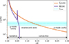 |
Fig. 1. Propagation diagram of the inner 30% of a red giant model with M = 1.25 M⊙, Z = 0.020. Characteristic frequencies |


 (9)
(9)
 (10)
(10)
where ρ is the local density of stellar material, and ρin is the average density of the spherical volume within the radius at which it is evaluated. The characteristic frequencies S and N are functions of fundamental stellar structure parameters such as the density ρ, the pressure p, the gravitational acceleration g, the local sound speed c, the adiabatic coefficient Γ1, and the gradients with respect to the radius coordinate r thereof. In oscillation cavities, k2 > 0 denotes the square of the radial wave vector, and conversely, in evanescent zones, k2 < 0 corresponds to the squared exponential decay length of the general radial solution x(r)∝eikr. The transmission coefficient in the weak-coupling approximation Tw is therefore given by the e-foldings across the evanescent zone,
 (11)
(11)
where the limits of the integral are the inner (rin) and outer (rout) boundaries of the evanescent zone (i.e., zeros of k2). Applying a Taylor expansion to Eq. (7) (since Tw is expected to be small) and inserting Eq. (11) for T, we obtain the expression found by Shibahashi (1979) (although via different reasoning) for the coupling strength in the weak-coupling limit,
 (12)
(12)
which we refer to as weak coupling in the following.
Takata (2016a) derived the transmission coefficient in the strong-coupling approximation. The treatment of the singularities in the oscillation equations at rin, out introduces an additional term to the transmission coefficient in this limit,
 (13)
(13)
which we here abbreviate as ∇2(r0) to indicate that it is a positive term containing gradients of the characteristic frequencies, which need to be evaluated at a radius r0 located in the middle of the evanescent zone (for the full expression for ∇2 as a function of radius, cf. Appendix A). ∇2(r0)≥0 implies that Ts ≤ Tw. Physically, this means that the behavior of oscillations around the turning points suppresses the coupling further from the exponential decay over the width of the evanescent zone. This expression was derived explicitly assuming a narrow evanescent zone, however, such that both turning points affect the form of the wave function simultaneously, and the contribution from ∇2(r0) is comparable with that from the decay length, while this effect is overestimated when the evanescent zone becomes too wide. Inserting Eq. (13) into the general expression Eq. (7), we obtain what we call the strong coupling,
 (14)
(14)
Since both expressions have been derived in the framework of asymptotic analysis, they share the underlying assumption that the stellar structure (in particular, the characteristic frequencies) vary only slowly across the evanescent zone compared to the local decay length. Because Ts contains gradients of  and
and  , however, the value of the strong coupling is more severely affected by the violation of this assumption.
3. Methods
3.1. Stellar models
We calculated multiple models on the RGB along seven tracks with masses1M ∈ {1.00, 1.25, 1.50, 1.75, 2.00} M⊙ (for Z = 0.02) and initial metallicities Z ∈ {0.015, 0.020, 0.025} (for M = 1.25 M⊙) using version r24.08.1 of the publicly available stellar evolution code MESA (“Modules for Experiments in Stellar Astrophysics”; Paxton et al. 2011, 2013, 2015, 2018, 2019; Jermyn et al. 2023). We chose standard input physics, including the solar composition described by Grevesse & Sauval (1998), and we neglected rotation, overshooting, and magnetic fields. We added a slight artificial diffusion to smooth the profiles, however, which improved the calculation of the strong coupling (cf. Sect. 3.2). We ensured that this did not significantly affect the evolution of the stars2. The output of the models notably contained values for ρ, p, g, Γ1, c, S, N, and the polytropic index  along the radial profile of the star, as well as global parameters such as the luminosity L, the effective temperature Teff, and an estimate for νmax from the scaling relation Eq. (1). In Fig. 2 we show the computed tracks in Hertzsprung-Russel diagrams.
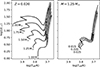 |
Fig. 2. Evolutionary tracks of stars with various masses M at an initial metallicity Z = 0.020 (left) and various Z at M = 1.25 M⊙ (right). The circles mark the positions of the models for which we evaluated the coupling strength. |
The profile data served as input to the stellar oscillation code GYRE (Townsend & Teitler 2013), which we used to solve the oscillation equations numerically and to compute the order, degree, and eigenfrequency of modes at which the star can resonate. For each model, we calculated the radial (l = 0) and dipole (l = 1) modes within [νmax − 3Δν, νmax + 3Δν], with an estimate for Δν from the sound-crossing time. Since the numeric solution does not rely on asymptotic approximations, we regarded it as an independent way to obtain oscillation frequencies and refer to them as observed frequencies.
3.2. Calculating the coupling strength
With the characteristic frequencies, the sound speed, and the density as a function of radius given from the models, we calculated the squared asymptotic radial wave vector k2 according to the dispersion relation Eq. (8) and determined its zeros via sign changes. Discarding zeros close to the stellar center or surface (and potentially those from the spike in the Brunt-Väisälä frequency, i.e., the sharp feature in  in Fig. 1 arising from the mean molecular weight discontinuity caused by the first dredge-up), we identified the remaining two as the limits of the evanescent zone. The integral in Eqs. (12) and (13) can then beapproximated by a Riemann sum between these turning points.
The calculation of the gradient term ∇2 as a function of the radius coordinate is outlined in Appendix A. With the turning points identified as above, we were also able to calculate  according to Eq. (A.1). We then used the two grid points in the stellar profile with radius coordinates closest to r0 to estimate ∇2(r0) by linear interpolation between them. When the spike in the Brunt-Väisälä frequency lies in the evanescent zone, the steep variation in the characteristic frequency and the additional zeros in k2 violate the underlying assumption of smooth variations in the stellar structure and make it impossible to evaluate this term meaningfully (cf. Jiang 2022 for a detailed analysis of the effects), and hence, we did not attempt to calculate qs for frequencies where this was the case. To investigate the effect of the Brunt-Väisälä-spike on the weak coupling and the evolution of the strong coupling without this feature, we evaluated the two couplings a second time for each model after we removed the spike by linearly interpolating N2 and the polytropic index between the spike base-points.
With the integral and gradient terms evaluated in these ways, we calculated qw and qs for each model, for the corresponding νmax, and for all dipole-mode frequencies identified by GYRE that we used in the asymptotic fit described in the following section. In this way, we probed the frequency dependence of k2 and its zeros (cf. Eq. (8)).
3.3. Asymptotic fitting
Starting from the mixed-mode resonance condition Eq. (4), we derived an asymptotic formula for the period of mixed modes following the arguments by Christensen-Dalsgaard (2012), which were used in a similar way by Hekker et al. (2018). Inserting the definitions Eqs. (5, 6) into Eq. (4) and rearranging the terms, we obtain
![Mathematical equation: $$ \begin{aligned} \Pi _\mathrm{as} =\Delta \Pi \cdot \left(-n_\mathrm{pg} +\epsilon _\mathrm{g} +\frac{1}{2}-\frac{\arctan \left[q\cot \left(\pi \left(\frac{\nu }{\Delta \nu }-\epsilon _\mathrm{p} \right)\right)\right]}{\pi }+n_\mathrm{p} \right)\,, \end{aligned} $$](/articles/aa/full_html/2025/08/aa55255-25/aa55255-25-eq26.gif) (15)
(15)
where the periodicity of the tangent function with mπ, m ∈ ℤ is used to replace ng by the more straightforward total radial order npg = np + ng, which always increases by 1 for the mode with the same degree and the next higher eigenfrequency (when all consecutive modes are present in the sample). The addition of the acoustic radial order np lifts the degeneracy (that is introduced when the tangent of the expression is inverted) in such a way that Πas becomes a smooth function of ν. Since np is sometimes misassigned by GYRE, we replaced it by a parameter nφ that explicitly fulfills this purpose by defining
 (16)
(16)
where the index i labels the observed modes in order of ascending eigenfrequency, and ![Mathematical equation: $ \varphi=\arctan\left[q\cot\left(\pi\left(\frac{\nu}{\Delta\nu}-\epsilon_{\mathrm{p}}\right)\right)\right] $](/articles/aa/full_html/2025/08/aa55255-25/aa55255-25-eq28.gif) .
.
In observations, the radial orders npg and np, 0 would be unknown and would therefore appear as free parameters. Working with models, however, we were able to treat them as given quantities, just as the eigenfrequencies. The five remaining parameters are {qas, Δν, ΔΠ, ϵp, ϵg}, where we refer to the coupling strength obtained from the asymptotic periods as asymptotic coupling. We fit for the five free parameters by minimizing the χ2-sum
![Mathematical equation: $$ \begin{aligned} \chi ^2=\sum \limits _i\left[\frac{1}{\nu _i}-\Pi _\mathrm{as} (\nu _i,n_{\mathrm{pg} ,i},n_{\varphi ,i};q_\mathrm{as} ,\Delta \nu ,\Delta \Pi ,\epsilon _\mathrm{p} ,\epsilon _\mathrm{g} )\right]^2 \end{aligned} $$](/articles/aa/full_html/2025/08/aa55255-25/aa55255-25-eq29.gif) (17)
(17)
over the modes i we found for each model.
This χ2-sum has multiple local minima. The parameters are also strongly correlated. These two facts make a numerical optimization difficult because the minimization algorithm can converge to a local instead of to the global minimum in one parameter, which then also affects the values of the other parameters. To circumvent this, we performed multiple optimizations per model with varying initializations. The flowchart in Fig. 3 visually represents the fitting procedure outlined in the following paragraphs.
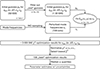 |
Fig. 3. Flowchart outlining our fitting procedure. |
From the distributions specified in Table 1, we drew 50 000 sets of initial guesses for the parameters. To save computation time, we only kept those that corresponded to a sufficiently low initial χ2 sum,
Properties of the initial-guess sampling.
 (18)
(18)
that is, the average deviation was no larger than 3% of the period corresponding to the mean frequency of the sample ⟨ν⟩. Typically, these were still about 30 000 sets. To avoid chance alignments and simulate observational noise, we also applied a Monte Carlo sampling with a standard deviation of 0.01 μHz and 100 realizations to the observed frequencies. For each combination of initial parameter guesses and perturbed frequencies, we then used the curve_fit function included in the Python package scipy.optimize with the implementation of the dogbox algorithm to minimize the χ2 sum Eq. (18). To ensure that all local minima were sampled, we only allowed the parameters Δν and ΔΠ, which are most strongly subjected to aliasing, to vary by ±0.5% from the initial guess. In turn, we set the tolerance for the termination of the algorithm rather high, which had the side effect that the fit sometimes converged too early close to the limits. This especially affected the fitting for qas, which has a hard limit at 0. In models in which the actual value of q was low (lower than ∼0.1), the χ2 sum of these limit convergences can become comparable to the global minimum, and it therefore affected the statistics of the best-fit distributions. To avoid errors from this effect, we only accepted fits that converged to qas ≥ 5 ⋅ 10−3 for further consideration.
We subsequently normalized the optimized χ2 sum to make it more comparable among the different models. As an estimate for the degrees of freedom, we used the number of modes available to the fit Nmodes minus the number of expected modes per acoustic order, which define the shape of the mixed-mode pattern and therefore needed to be fixed, while the availability of multiple acoustic orders introduced the redundancy that allowed the fit to improve. Since the width of an acoustic order is given by Δν, we approximated the latter by
 (19)
(19)
to give the normalized χ2 sum
 (20)
(20)
This normalization would also disfavor aliases arising from oversampling of the modes if the npg were unknown because the higher chance for some of the asymptotic modes to align well with the observed modes at a higher density of mixed modes would be counteracted by the increase in NΔν. By this normalized  sum, we selected the 100 best fits (i.e., those with the lowest
  ) and calculated the final estimate of the fit parameters as the median of their distribution among this best subset, with uncertainties as the difference to the first and third quartile, respectively.
4. Results
In Fig. 4 we show the results of the computations outlined in Sect. 3 for a modeled star with M = 1.25 M⊙ and Z = 0.02 along its evolution up the RGB. The coupling was evaluated for the models indicated with circles in the Hertzsprung-Russel diagram in Fig. 2. Since a star ascending the RGB expands in radius at (nearly) constant mass, νmax decreases with evolution, meaning that the star moves from right to left in the figure. We visually analyzed the trends in this and similar figures to discuss our results.
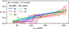 |
Fig. 4. Values of the coupling strength q computed in the three ways presented in Sect. 3 as a function of νmax for stellar models with M = 1.25 M⊙, Z = 0.020 along the RGB. The star evolves from right to left. The solid lines represent qw(νmax) (dark blue for the full profile, and light blue for profile without the N2 spike) and qs(νmax) (red for the full profile, and purple without the spike), and the shaded areas show the range of values we calculated for the frequencies in the sample used for the fit. The green markers show qas with the uncertainties as described in Sect. 3.3. Below 100 μHz, the x-axis ticks show spacings of 10 μHz; above 100 μHz, the major ticks show spacings of 100 μHz and the minor ticks continue in steps of 10 μHz. The arrow indicates the model that is further analyzed in Fig. 10. |
4.1. Applicability of the approximations
The asymptotic coupling initially agrees with the values predicted in the strong-coupling approximation. Where the ranges of qw and qs overlap, qas is in some cases also consistent with the weak-coupling approximation. Coming from high values on the subgiant branch, the data show that the asymptotic coupling follows qs along the early RGB (for νmax ≳ 110 μHz), even when the reduction of the transmitted mode energy due to the second term in Eq. (13) is so strong that qs < qw. In more evolved models (νmax ≲ 70 μHz), the strong coupling has very low values. The data points show, however, that the weak-coupling approximation is more appropriate to reproduce the coupling observed in the mixed-mode pattern in this regime.
In intermediate models (110 μHz ≳ νmax ≳ 70 μHz), qs could not be calculated from the full stellar profile because of the spike in the Brunt-Väisälä frequency (as discussed in Sect. 3.2). A removal of the spike revealed that the strong coupling drops quite steeply. The time step at which this drop occurs depends on the frequency, which explains the wide range of values of qs in this regime, as represented by the purple shaded area.
The weak coupling gives a good estimate for the asymptotic values in this intermediate regime. The comparison of qw for profiles with and without the spike shows that the spike mainly increases the integral over the decay length  , and it hence gradually decreases the coupling as it moves up through the evanescent zone. When νmax falls below
  at the base of the spike, the evanescent zone abruptly narrows, and qw steps up to agree with the spike-free value again. The deviation is marginal compared to the range given by the frequency dependence, however.
When the asymptotic coupling is consistent with the strong-coupling approximation, the fit values mostly fall close to the middle of the range in coupling strengths qs evaluated at the different frequencies. They tend to lie closer to the upper end of the shaded area when they follow the weak coupling, however.
4.2. Mass and metallicity dependence
While the mass of the red giant affects the value of the coupling as a function of νmax (cf. Fig. 5), the overall trend stays the same: Coming from the subgiant branch, where the coupling can reach very high values, qas continues to closely follow the strong-coupling approximation as long as the calculation in this limit is still possible. The models without the spike also show a similar behavior as those with the spike. We therefore omitted the results of the former for clarity.
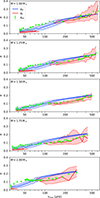 |
Fig. 5. Values of the coupling strength q as a function of frequency of maximum oscillation power νmax for RGB models with different masses M, as indicated in each panel, and the initial metallicity Z = 0.020. Cf. Fig. 4 for the meaning of the colors and symbols. Stars evolve from right to left. |
With increasing mass, the onset of the RGB phase occurs at lower νmax because the corresponding radius also increases. On the lower RGB, the coupling strength is lower for a higher stellar mass at the same νmax. To rule out that this effect is solely due to the radius evolution as well, we plotted q as a function of the evanescent zone width in terms of the number of asymptotic e-foldings W,
 (21)
(21)
Figure 6 shows that for the same width W, the coupling indeed tends to be weaker in higher-mass stars on the early RGB (most prominently at W ∼ 0.2). With qw(νmax) being a mass-independent function of W as per Eq. (12), the blue line can serve as a good visual reference.
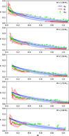 |
Fig. 6. Values of the coupling strength q as a function of evanescent zone width W for RGB models with different masses M, as indicated in each panel, and the initial metallicity Z = 0.020. Cf. Fig. 4 for the meaning of the colors and symbols. Stars evolve from left to right. |
As soon as the calculation of the strong-coupling approximation breaks down due to the spike in the Brunt-Väisälä frequency, all models in the mass range we considered can be described using the weak-coupling approximation within three times the width of the uncertainties. While the νmax at which this transition occurs varies with mass (cf. Fig. 5), the corresponding evanescent zone width is fairly constant at W ∼ 0.4 (cf. Fig. 6).
Metallicity does not significantly influence the coupling strength of dipolar mixed modes in red giants. Figure 7 shows that the evolution of q is very similar for the three 1.25 M⊙ models calculated with different initial metallicities.
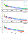 |
Fig. 7. Values of the coupling strength q as a function of evanescent zone width W for RGB models with different initial metallicities Z, as indicated in each panel, and the mass M = 1.25 M⊙. Cf. Fig. 4 for the meaning of the colors and symbols. Stars evolve from left to right. |
5. Discussion
In agreement with, for example, Pinçon et al. (2020), Jiang et al. (2022), we find that along the RGB the coupling strength generally decreases with evolution. While the evanescent zone lies in the radiative layer above the hydrogen-burning shell, the asymptotic coupling is consistent with the values predicted in the strong-coupling approximation. When the evanescent zone is located at the bottom of the convective envelope, qas is well described by the weak coupling. Although this distinction by the radiative or convective nature of the evanescent zone is not directly visible in the results presented in Figs. 4–7, we can infer the two regimes discussed from the transient of the spike in the Brunt-Väisälä frequency (which is visible in the figures from the fact that we cannot calculate qs when it lies in the evanescent zone). Since the spike forms at the deepest extent of the convective envelope and the evanescent zone moves outward during evolution, the latter must lie in the radiative layer before the spike appears. After it has passed through, the evanescent zone is predominantly convective because the convective envelope has not receded much by this point (van Rossem et al. 2024). This assumption is supported by the analysis of the relevant stellar profiles, for instance, in Fig. 1 for the model with νmax ∼ 55 μHz in Fig. 4. Considering that  in convective regions because it is related to the Schwarzschild criterion for convection, this propagation diagram shows that most of the evanescent zone in this model is convective for the considered frequency range.
While Pinçon et al. (2020) argued there should be an intermediate regime in which none of the two approximations holds, our model calculations suggest that the range of qw agrees with qas (within three times the uncertainties at most) as soon as the width of the evanescent zone W ≥ 0.4 in units of the local decay length. For W < 0.4, qs can still be calculated for at least some frequencies in the observable range. We therefore suggest a selection of the coupling formula to use as described by
 (22)
(22)
The quality of this selection for our models is shown in Fig. 8, which demonstrates the good agreement of the theoretical with the observed values using this straightforward prescription. The cutoff of W = 0.4 corresponds to a weak coupling of qw ∼ 0.11 following Eq. (12).
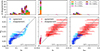 |
Fig. 8. Comparison of the coupling strengths obtained via asymptotic fitting and theoretical calculations. From left to right, the theoretical prescription used is the weak coupling, strong coupling, and the selection of one of the two as given by Eq. (23). Bottom row: qas (with uncertainties as described in Sect. 3.3) on the y-axis vs. theoretical values (the error bars indicate the range across the fitted frequencies) on the x-axis. Models that agree with the one-to-one line (gray diagonal) within the error bars are shown in dark blue resp. red for qw resp. qs, and those that disagree are shown in light blue resp. purple. Percentages relative to the total number of models we fit. Top row: histograms of the distribution of disagreeing models over the theoretical coupling values. The stacked-up colors represent models of different masses as indicated in the legend. |
The values of observables such as νmax corresponding to the W = 0.4 cutoff depend on the mass: The transition occurs at lower νmax for higher masses (cf. Fig. 9). The dependence is nonlinear. Metallicity might also affect the value of νmax at which W = 0.4, albeit less strongly. These dependences make it difficult to determine whether the evanescent zone of an observed red giant is radiative or convective. Because the variation of q with evolution is rather slow in this regime, the use of Eq. (23) to observationally differentiate the two stages is also limited.
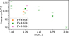 |
Fig. 9. Values of νmax corresponding to models with threshold evanescent zone width as a function of stellar mass (M = 1.25 M⊙ markers are slightly offset for clarity). The horizontal bars show νmax of the models with W closest to 0.4 on either side, and crosses show the linearly interpolated values for W = 0.4. The metallicity is distinguished by color, as indicated in the legend. |
5.1. Strong coupling
The lower values of qs in an equal evanescent zone width W for more massive stars can be explained by the fact that, owing to the larger extent of the convective core on the main sequence, a higher proportion of the stellar mass is confined to the inert helium core of the red giant. As the core contracts and the envelope expands along the RGB, this means that the gradient  is more strongly negative in the evanescent zone of more massive stars (which lies in the expanding region and therefore has a lower density than the core). This increases the gradient of the modified Brunt-Väisälä frequency in Eq. (A.4), and thus, increases the second term in Eq. (13).
Across all masses and metallicities we considered, the width of the red shaded area at small W ≤ 0.4 (i.e., on the early RGB) is rather large. This is not due to the real frequency dependence of qs, but rather to numerical noise along the stellar radial profile that affects the evaluation of the gradient term in Eq. (13). This is also the reason for the nonmonotonous evolution of qs with νmax or even W. Since a shift in frequency also shifts the turning points rin, out and thus r0, where the gradients are evaluated, the centroid of the shaded area can be seen as an estimate for the true strong-coupling value, which reproduces the behavior of qas well in this regime. This is expected because the evanescent zone lying in the radiative layer immediately above the hydrogen-burning shell is very narrow during this phase (van Rossem et al. 2024).
At the bottom of the convective envelope,  abruptly falls below zero. This drop in the Brunt-Väisälä frequency (while the Lamb frequency maintains a similar power-law shape to what it was below the envelope; cf. Fig. 1) means that the evanescent zone widens rapidly (i.e., W increases), which means that the weak-coupling approximation becomes applicable (Pinçon et al. 2020). Meanwhile, the second term in Eq. (13) remains of the same order of magnitude, so that Ts is still strongly suppressed compared to Tw. The steep gradient of
  around the bottom of the convection zone (which remains the inner turning point rin) actually even increases ∇2 everywhere between the turning points. This implies that the suppression of Ts below Tw is even stronger when the evanescent zone lies in the convective envelope. This explains why the drop of qs is quite sudden when the evanescent zone moves into the convective envelope, as shown for the models without the spike in Fig. 4.
5.2. Weak coupling
In models with a convective evanescent zone, the asymptotic coupling strength tends to fall closer to the maximum of qw calculated from the frequency sample than to the central value. This can be due to both an error in the weak-coupling approximation and an incompleteness in the asymptotic formula (15), which does not account for the frequency dependence of the coupling (cf. also Jiang et al. 2020). As discussed by Pinçon et al. (2020) (and also shown in Fig. 4 by the width of the blue shaded area), the frequency dependence of the weak coupling is much stronger for evanescent zones that lie in the convective envelope because of the radial profile of the characteristic frequencies shown in Fig. 1: In the radiative zone, both characteristic frequencies have a similar slope, and thus, the width of the evanescent zone only changes little with a change in frequency. At the bottom of the convective envelope, however, the steep slope of the Brunt-Väisälä frequency keeps the inner turning point almost fixed when the frequency changes. Thus, modes at slightly higher frequencies already have a substantially narrower evanescent zone, and they are therefore more strongly coupled. Since the asymptotic formula treats qas as a frequency-independent parameter, the fit converges to some average value.
To assess whether this average is biased toward higher frequencies, we performed fits to two subsets of modes: A subset with a frequency below the 75th and another subset above the 25th percentile of the full sample by number of dipole modes. Fig. 10 shows that the fit over the full frequency range indeed lies significantly closer to the fit that only includes the higher frequencies. This suggests that these dominate the χ2 sum (Eq. (18)) for the variation in qas, which leads to a convergence to a parameter set with qas systematically higher than qw(νmax). This can be explained by the fact that at higher frequencies, the number of mixed modes per acoustic order is lower (cf. also Eq. (20)), and therefore, there are more orders (contributing to the average) in a sample with the same number of modes. This suggests that in order to match the observed coupling strengths in the weak-coupling regime, it is advisable to calculate qw not at νmax, but rather at a frequency close to the maximum of the observed range. At the same time, it is clear that the error introduced by the assumptions of a wide evanescent zone (e.g., the Taylor expansion of Eq. (7) and the neglect of the behavior of k at the turning points in Tw) affects the more strongly coupled modes with higher frequencies more. The systematic offset of qas from qw(νmax) is therefore a combined effect of the ignored frequency dependence and incompleteness of the weak-coupling approximation. For some models with very weak coupling, qas falls below qw(νmax) against this general trend. These might still be subject to the effect of limit convergences, which become very difficult to distinguish from the statistics of the actual best-fit subset.
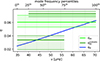 |
Fig. 10. Coupling strength for the model marked with an arrow in Fig. 4 as a function of mode frequency. The fit values qas were fit to modes in the frequency range indicated by the width of the marker, and the uncertainties were estimated as described in Sect. 3.3. The solid dark blue line shows the weak coupling calculated as per Eq. (12). The vertical dotted lines indicate the frequencies of the model’s radial modes. |
The fact that the weak coupling can be used already for W ∼ 0.4 is somewhat fortuitous because for a value of q ∼ 0.1, the Taylor expansion used in Eq. (12) alone deviates by ∼25% from the full expression. This underestimates qw for a given transmission coefficient Tw. It appears, however, that this roughly cancels with the fact that neglecting the turning points compared to the derivation by Takata (2016a) overestimates the transmission coefficient in these narrow evanescent zones. This empirical result simplifies the calculation of the coupling strengths enormously. We note that the error of this result depends on the mass: The agreement is worst for M = 2.00 M⊙ (cf. Fig. 6), where qas systematically deviates from the highest qw by up to three times of the uncertainties for models with 0.6 ≲ W ≲ 0.9. Therefore, we cannot expect to be able to apply this result to stars with even higher masses. The cancellation of the aforementioned effects works best for our tracks with masses of 1.50 M⊙ and 1.75 M⊙ (cf. top row of Fig. 8). While the actual effect of the turning points is hard to quantify (for this reason, only the coupling prescriptions in the limits of explicitly wide and narrow evanescent zones have been derived so far), it is clear that it depends on the stellar structure in a different way than the quality of the Taylor expansion, which is determined by W alone. This different dependence allows the quality of the cancellation to vary with stellar mass in the way we observe it: The error introduced by the Taylor expansion is larger than the error from the neglect of the turning points in the models with M ∈ {1.00, 2.00} M⊙, while they are similar in models with masses in between.
In principle, while the spike at the mean molecular weight discontinuity lies in the evanescent zone, it should act as another buoyancy cavity in which the mode energy can be trapped; in the practical calculation of qw, however, we ignored it and integrated  across the spike, as if the mode also decayed there. Fig. 4 shows that this effect is small, which can be explained by the fact that the spike is significantly narrower than k−1. We therefore conclude that it is not necessary to adapt the stellar profiles when calculating the coupling strength because the strong-coupling approximation no longer adequately describes the evolution of the coupling when the spike becomes relevant anyway, and the value of the weak coupling is only marginally affected. The asymptotic coupling values might follow a similar evolution as qw in response to the chemical discontinuity that causes the spike. The temporary increase in qas as the spike leaves the evanescent zone is most notable for the 1.75 M⊙ track (cf. fourth panel of Fig. 5). This feature is not significant compared to the uncertainties of the values, however, and further studies are needed to investigate this behavior.
6. Conclusion
We empirically verified that the validity regimes in which the strong- and weak-coupling approximations are applicable on the RGB coincide with the evanescent zone being fully radiative and convective, respectively (as discussed by, e.g., Pinçon et al. 2020; Jiang et al. 2022. The left two columns of Fig. 8 show that the theoretical couplings agree well with the asymptotic values in the respective regimes, while qw overestimates the coupling when the model lies in the strong-coupling regime and qs underestimates the coupling when it is weak. This is also consistent with Jiang et al. (2022), for example, who reported qualitatively similar results (cf. Fig. 5 of that paper) for their order-wise fitting approach. We also showed that for the transition from one limit to the other, no additional prescription is needed to approximate the fit values using the stellar structure within the considered mass range. To explore this simplification in coupling strength calculation further, we found the evanescent zone width W (in units of local decay length) as a straightforward mass-independent parameter of the stellar structure to differentiate between the two regimes: For narrow evanescent zones with W ≤ 0.4 e-foldings, the strong coupling (evaluated at frequencies for which the Brunt-Väisälä spike does not lie in the evanescent zone) approximates the asymptotic coupling strength well; above (W > 0.4), the weak coupling can be used as an estimate in the mass range we considered here (1.00 M⊙ ≤ M ≤ 2.00 M⊙). This conclusion is supported by the good agreement of qsel (introduced in Eq. (23)) with qas, as shown in the bottom right panel of Fig. 8. It adds to the observation by Jiang et al. (2022) (who also found that the frequency-fit coupling strength typically aligns with one of the theoretical values) by adding an independent constraint on which approximation to use.
We emphasize that the applicability of the weak-coupling approximation at these small evanescent zone widths is purely empirical and relies on the serendipitous cancellation of different assumptions. We do not expect it to necessarily hold for stellar models with masses outside the range we studied here, especially because the agreement is worst for the models along the lowest- and highest-mass evolutionary tracks (cf. top right panel of Fig. 8). Still, these findings can aid future work because they offer a possibility to estimate the coupling strength in a straightforward way. This is a key ingredient for the asymptotic calculation of mixed modes.
We further demonstrated that it is beneficial to calculate the coupling across a frequency range rather than just for νmax in both limits: Noise that appears in the evaluation of the strong coupling can be treated by taking a suitable average of qs over the frequency range; and calculating the weak coupling at frequencies close to the upper limit of the frequency range sampled by observations increases the agreement with the values found from the mixed-mode pattern (which typically assumes qas to be a frequency-independent parameter), as we showed in the bottom right panel of Fig. 8 from the fact that most theoretical values qsel lie left of the one-to-one line in the regime of weak coupling. On the other hand, no explicit treatment (or removal) of the spike in the Brunt-Väisälä frequency caused by the chemical discontinuity left behind by the first dredge-up is required when calculating the coupling strength in an RGB model.
We also tested the influence of the stellar mass on the evolution of the coupling: In the strong-coupling regime, q tends to be lower for higher masses because the gradient of the modified Brunt-Väisälä frequency is steeper. The mass also affects the evolution of νmax in relation to the evanescent zone width W, which is more relevant for the calculation of the coupling strength. Except for the stronger suppression on the early RGB, q evolves as a function of W almost independent of mass or metallicity.
Since mass loss is negligible during the evolutionary phases up to the most evolved model we studied, we did not consider it in our models.
Our MESA inlists and run_star_extras.f90 are publicly available on Zenodo (doi: https://doi.org/10.5281/zenodo.15261756)
Acknowledgments
We thank Chen Jiang for refereeing this paper and helping increase its clarity and rigor with useful comments. We also thank Nicholas Proietti for contributing ideas to the start of the project. The research leading to the presented results has received funding from the European Research Council Consolidator Grant DipolarSound (grant agreement No. 101000296).
References
- Christensen-Dalsgaard, J. 2012, in Progress in Solar/Stellar Physics with Helio- and Asteroseismology, eds. H. Shibahashi, M. Takata, & A. E. Lynas-Gray, ASP Conf. Ser., 462, 503 [NASA ADS] [Google Scholar]
- Grevesse, N., & Sauval, A. J. 1998, Space Sci. Rev., 85, 161 [Google Scholar]
- Hekker, S., & Christensen-Dalsgaard, J. 2017, A&ARv, 25 [Google Scholar]
- Hekker, S., Elsworth, Y., & Angelou, G. C. 2018, A&A, 610, A80 [NASA ADS] [CrossRef] [EDP Sciences] [Google Scholar]
- Jermyn, A. S., Bauer, E. B., Schwab, J., et al. 2023, ApJS, 265, 15 [NASA ADS] [CrossRef] [Google Scholar]
- Jiang, C. 2022, Astron. Nachr., 343, e20220051 [Google Scholar]
- Jiang, C., Christensen-Dalsgaard, J., & Cunha, M. 2018, MNRAS, 474, 5413 [Google Scholar]
- Jiang, C., Cunha, M., Christensen-Dalsgaard, J., & Zhang, Q. 2020, MNRAS, 495, 621 [Google Scholar]
- Jiang, C., Cunha, M., Christensen-Dalsgaard, J., Zhang, Q. S., & Gizon, L. 2022, MNRAS, 515, 3853 [NASA ADS] [CrossRef] [Google Scholar]
- Kjeldsen, H., & Bedding, T. R. 1995, A&A, 293, 87 [NASA ADS] [Google Scholar]
- Mosser, B., Goupil, M. J., Belkacem, K., et al. 2012, A&A, 540, A143 [NASA ADS] [CrossRef] [EDP Sciences] [Google Scholar]
- Mosser, B., Pinçon, C., Belkacem, K., Takata, M., & Vrard, M. 2017, A&A, 600, A1 [NASA ADS] [CrossRef] [EDP Sciences] [Google Scholar]
- Paxton, B., Bildsten, L., Dotter, A., et al. 2011, ApJS, 192, 3 [Google Scholar]
- Paxton, B., Cantiello, M., Arras, P., et al. 2013, ApJS, 208, 4 [Google Scholar]
- Paxton, B., Marchant, P., Schwab, J., et al. 2015, ApJS, 220, 15 [Google Scholar]
- Paxton, B., Schwab, J., Bauer, E. B., et al. 2018, ApJS, 234, 34 [NASA ADS] [CrossRef] [Google Scholar]
- Paxton, B., Smolec, R., Schwab, J., et al. 2019, ApJS, 243, 10 [Google Scholar]
- Pinçon, C., Goupil, M. J., & Belkacem, K. 2020, A&A, 634, A68 [Google Scholar]
- Shibahashi, H. 1979, PASJ, 31, 87 [NASA ADS] [Google Scholar]
- Takata, M. 2006, PASJ, 58, 893 [Google Scholar]
- Takata, M. 2016a, PASJ, 68, 109 [NASA ADS] [CrossRef] [Google Scholar]
- Takata, M. 2016b, PASJ, 68, 91 [NASA ADS] [CrossRef] [Google Scholar]
- Tassoul, M. 1980, ApJ, 43, 469 [Google Scholar]
- Townsend, R. H. D., & Teitler, S. A. 2013, MNRAS, 435, 3406 [Google Scholar]
- van Rossem, W. E., Miglio, A., & Montalbán, J. 2024, A&A, 691, A177 [NASA ADS] [CrossRef] [EDP Sciences] [Google Scholar]
Appendix A: Strong coupling approximation
In the strong coupling approximation, the evanescent zone is assumed to be so narrow that the behavior of a structure perturbation near the zeros of the asymptotic wave vector k2 (cf. Eq. (8)) becomes relevant to the overall behavior of the mode. Since the oscillation equations show singularities at these points, Takata (2016a) introduces a change of coordinates such that the dependent variables become complex and solutions can be derived. The corresponding independent (radius) variable s is defined by
 (A.1)
(A.1)
where rS, N are the turning points where  , respectively. The identification with rin, out depends on the choice of oscillation frequency and model, since they determine whether ω2 crosses
  or
or  first. On the RGB, typically rin = rN, rout = rS (cf. Fig. 1). The radius r0 as it appears in Eq. (13) is defined by s(r0) = 0.
Upon relating the solutions in this frame of coordinates back to physical quantities and using an order-of-magnitude argument that explicitly requires the coupling to be strong, Takata (2016a) finds expression (13) for the transmission coefficient, where
![Mathematical equation: $$ \begin{aligned} \nabla ^2(r_0)=\frac{\pi }{2}\left[\sqrt{\frac{s_0^2-s^2}{\mathcal{P} \mathcal{Q} }}\left(\frac{\mathrm{d} \ln \mathfrak{c} }{\mathrm{d} s}\right)^2\right]_{s = 0}\,. \end{aligned} $$](/articles/aa/full_html/2025/08/aa55255-25/aa55255-25-eq49.gif) (A.2)
(A.2)
For a wide evanescent zone, the shape of the wave function would change and this term would no longer appear in leading order and hence, the suppression of Ts is overestimated.
The reference coordinate s0 is given by
 (A.3)
(A.3)
and can be both positive or negative. The gradient  contains multiple terms:
 (A.4)
(A.4)
In this expression,
 (A.5)
(A.5)
relate to the modified Lamb and Brunt-Väisälä frequency in the new coordinate frame, respectively, and therefore
 (A.6)
(A.6)
correspond to the two bracketed terms in the asymptotic dispersion relation Eq. (8) in terms of a dimensionless frequency
 (A.7)
(A.7)
This means that 𝒫 and 𝒬 are zero at rS, N, respectively, and therefore their logarithmic derivatives appearing in Eq. (A.4) diverge at the limits of the evanescent zone, which demonstrates that  needs to span a vast range of values within this narrow region. Therefore, the noise created by numerically evaluating the many gradients of stellar structure would affect the value of the transmission coefficient (and hence qs) strongly.
To mitigate this, we used two equilibrium (static) equations of stellar structure to evaluate as many derivatives analytically as possible: The continuity equation
 (A.8)
(A.8)
where m(r) is the mass contained within radius r; and the equation of hydrostatic equilibrium
 (A.9)
(A.9)
Using these, we can write:
![Mathematical equation: $$ \begin{aligned} \mathcal{V}&= \frac{1}{\Gamma _1J}\frac{Gm\rho }{pr}\\ \mathcal{A}&= \frac{1}{J}\frac{Gm\rho }{pr}\underbrace{\left(\frac{\mathrm{d} \ln \rho }{\mathrm{d} \ln p}-\frac{1}{\Gamma _1}\right)}_{=: \Gamma _\mathcal{A} ^{-1}} \\ \frac{\mathrm{d} J}{\mathrm{d} r}&= \frac{\rho }{r\rho _{in}}\left(\frac{Gm}{r}\frac{\rho }{p}\frac{\mathrm{d} \ln \rho }{\mathrm{d} \ln p}-3J\right)\\ \frac{\mathrm{d} \ln \mathcal{P} }{\mathrm{d} \ln r}&= \frac{r}{\mathcal{P} }\left[2\frac{\mathrm{d} J}{\mathrm{d} r}-\omega ^2\frac{\rho r^2}{p}\frac{1}{\Gamma _1J}\left(\frac{Gm\rho }{pr^2}\left(1-\frac{\mathrm{d} \ln \rho }{\mathrm{d} \ln p}\right)\right.\right.\nonumber \\ &\qquad \left.\left.+\frac{2}{r}+\Gamma _1\frac{\mathrm{d} }{\mathrm{d} r}\left[\frac{1}{\Gamma _1}\right]-\frac{1}{J}\frac{\mathrm{d} J}{\mathrm{d} r}\right)\right]\\ \frac{\mathrm{d} \ln \mathcal{Q} }{\mathrm{d} \ln r}&= \frac{r}{\mathcal{Q} }\left[\frac{\mathrm{d} J}{\mathrm{d} r}-\frac{G^2}{\omega ^2}\frac{\rho m^2}{pr^4}\frac{1}{\Gamma _\mathcal{A} J}\left(\frac{Gm\rho }{pr^2}\left(1-\frac{\mathrm{d} \ln \rho }{\mathrm{d} \ln p}\right)+\frac{8\pi \rho r^2}{m}\right.\right.\nonumber \\ &\qquad \left.\left.-\frac{4}{r}+\Gamma _\mathcal{A} \frac{\mathrm{d} }{\mathrm{d} r}\left[\frac{1}{\Gamma _\mathcal{A} }\right]-\frac{1}{J}\frac{\mathrm{d} J}{\mathrm{d} r}\right)\right] \end{aligned} $$](/articles/aa/full_html/2025/08/aa55255-25/aa55255-25-eq59.gif) (A.10)
(A.10)
The remaining two gradients of the adiabatic index Γ1 and polytropic index  still need to be computed numerically as differential quotients. Since both quantities only vary slowly across the stellar profile, this is feasible – however, these terms still are the main source of noise, especially since the polytropic index being calculated from tabulated values for the equation of state is already subject to numerical noise itself.
All Tables
All Figures
|
Fig. 1. Propagation diagram of the inner 30% of a red giant model with M = 1.25 M⊙, Z = 0.020. Characteristic frequencies |
| In the text | |
|
Fig. 2. Evolutionary tracks of stars with various masses M at an initial metallicity Z = 0.020 (left) and various Z at M = 1.25 M⊙ (right). The circles mark the positions of the models for which we evaluated the coupling strength. |
| In the text | |
|
Fig. 3. Flowchart outlining our fitting procedure. |
| In the text | |
|
Fig. 4. Values of the coupling strength q computed in the three ways presented in Sect. 3 as a function of νmax for stellar models with M = 1.25 M⊙, Z = 0.020 along the RGB. The star evolves from right to left. The solid lines represent qw(νmax) (dark blue for the full profile, and light blue for profile without the N2 spike) and qs(νmax) (red for the full profile, and purple without the spike), and the shaded areas show the range of values we calculated for the frequencies in the sample used for the fit. The green markers show qas with the uncertainties as described in Sect. 3.3. Below 100 μHz, the x-axis ticks show spacings of 10 μHz; above 100 μHz, the major ticks show spacings of 100 μHz and the minor ticks continue in steps of 10 μHz. The arrow indicates the model that is further analyzed in Fig. 10. |
| In the text | |
|
Fig. 5. Values of the coupling strength q as a function of frequency of maximum oscillation power νmax for RGB models with different masses M, as indicated in each panel, and the initial metallicity Z = 0.020. Cf. Fig. 4 for the meaning of the colors and symbols. Stars evolve from right to left. |
| In the text | |
|
Fig. 6. Values of the coupling strength q as a function of evanescent zone width W for RGB models with different masses M, as indicated in each panel, and the initial metallicity Z = 0.020. Cf. Fig. 4 for the meaning of the colors and symbols. Stars evolve from left to right. |
| In the text | |
|
Fig. 7. Values of the coupling strength q as a function of evanescent zone width W for RGB models with different initial metallicities Z, as indicated in each panel, and the mass M = 1.25 M⊙. Cf. Fig. 4 for the meaning of the colors and symbols. Stars evolve from left to right. |
| In the text | |
|
Fig. 8. Comparison of the coupling strengths obtained via asymptotic fitting and theoretical calculations. From left to right, the theoretical prescription used is the weak coupling, strong coupling, and the selection of one of the two as given by Eq. (23). Bottom row: qas (with uncertainties as described in Sect. 3.3) on the y-axis vs. theoretical values (the error bars indicate the range across the fitted frequencies) on the x-axis. Models that agree with the one-to-one line (gray diagonal) within the error bars are shown in dark blue resp. red for qw resp. qs, and those that disagree are shown in light blue resp. purple. Percentages relative to the total number of models we fit. Top row: histograms of the distribution of disagreeing models over the theoretical coupling values. The stacked-up colors represent models of different masses as indicated in the legend. |
| In the text | |
|
Fig. 9. Values of νmax corresponding to models with threshold evanescent zone width as a function of stellar mass (M = 1.25 M⊙ markers are slightly offset for clarity). The horizontal bars show νmax of the models with W closest to 0.4 on either side, and crosses show the linearly interpolated values for W = 0.4. The metallicity is distinguished by color, as indicated in the legend. |
| In the text | |
|
Fig. 10. Coupling strength for the model marked with an arrow in Fig. 4 as a function of mode frequency. The fit values qas were fit to modes in the frequency range indicated by the width of the marker, and the uncertainties were estimated as described in Sect. 3.3. The solid dark blue line shows the weak coupling calculated as per Eq. (12). The vertical dotted lines indicate the frequencies of the model’s radial modes. |
| In the text | |
Current usage metrics show cumulative count of Article Views (full-text article views including HTML views, PDF and ePub downloads, according to the available data) and Abstracts Views on Vision4Press platform.
Data correspond to usage on the plateform after 2015. The current usage metrics is available 48-96 hours after online publication and is updated daily on week days.
Initial download of the metrics may take a while.