| Issue |
A&A
Volume 653, September 2021
|
|
|---|---|---|
| Article Number | A27 | |
| Number of page(s) | 14 | |
| Section | The Sun and the Heliosphere | |
| DOI | https://doi.org/10.1051/0004-6361/202141215 | |
| Published online | 03 September 2021 | |
Sunspot tilt angles revisited: Dependence on the solar cycle strength
1
School of Space and Environment, Beihang University, Beijing, PR China
e-mail: This email address is being protected from spambots. You need JavaScript enabled to view it.
2
Key Laboratory of Space Environment Monitoring and Information Processing of MIIT, Beijing, PR China
3
Key Laboratory of Solar Activity, National Astronomical Observatories, Chinese Academy of Sciences, Beijing 100101, PR China
4
School of Astronomy and Space Science, University of Chinese Academy of Sciences, Beijing, PR China
Received:
30
April
2021
Accepted:
28
May
2021
Abstract
Context. The tilt angle of sunspot groups is crucial in the Babcock-Leighton (BL) type dynamo for the generation of the poloidal magnetic field. Some studies have shown that the tilt coefficient, which excludes the latitudinal dependence of the tilt angles, is anti-correlated with the cycle strength. If the anti-correlation exists, it will be shown to act as an effective nonlinearity of the BL-type dynamo to modulate the solar cycle. However, some studies have shown that the anti-correlation has no statistical significance.
Aims. We aim to investigate the causes behind the controversial results of tilt angle studies and to establish whether the tilt coefficient is indeed anti-correlated with the cycle strength.
Methods. We first analyzed the tilt angles from Debrecen Photoheliographic Database (DPD). Based on the methods applied in previous studies, we took two criteria (with or without angular separation constraint Δs > 2.°5) to select the data, along with the linear and square-root functions to describe Joy’s law, and three methods (normalization, binned fitting, and unbinned fitting) to derive the tilt coefficients for cycles 21–24. This allowed us to evaluate different methods based on comparisons of the differences among the tilt coefficients and the tilt coefficient uncertainties. Then we utilized Monte Carlo experiments to verify the results. Finally, we extended these methods to analyze the separate hemispheric DPD data and the tilt angle data from Kodaikanal and Mount Wilson.
Results. The tilt angles exhibit an extremely wide scatter due to both the intrinsic mechanism for its generation and measurement errors, for instance, the unipolar regions included in data sets. Different methods to deal with the uncertainties are mainly responsible for the controversial character of the previous results. The linear fit to the tilt-latitude relation of sunspot groups with Δs > 2.°5 of a cycle carried out without binning the data can minimize the effect of the tilt scatter on the uncertainty of the tilt coefficient. Based on this method the tilt angle coefficient is anti-correlated with the cycle strength with strong statistical significance (r = −0.85 at 99% confidence level). Furthermore, we find that tilts tend to be more saturated at high latitudes for stronger cycles. The tilts tend to show a linear dependence on the latitudes for weak cycles and a square-root dependence for strong cycles.
Conclusions. This study disentangles the cycle dependence of sunspot group tilt angles from the previous results that were shown to be controversial, spurring confusion in the field.
Key words: Sun: magnetic fields / sunspots / Sun: activity / dynamo
© ESO 2021
1. Introduction
The line connecting the two polarities of a sunspot group usually tilts with respect to the east-west direction. The average tilt angle increases with increasing latitude, which is known as Joy’s law (Hale et al. 1919). Besides the systematic property, there is a large scatter of the individual tilt angles about the mean (Howard 1991b; Kitchatinov & Olemskoy 2011; Jiang et al. 2014a). One widely accepted mechanism characterizing Joy’s law is that the Coriolis force acts on toroidally oriented flux tubes in the north-south direction as they rise buoyantly to the surface through the convection zone (D’Silva & Howard 1993; Fisher et al. 1995; Caligari et al. 1995). Convective turbulent buffeting on the rising flux tube generates the tilt scatter (Longcope et al. 1996; Weber et al. 2012). Alternatively, it has been suggested that the tilt represents a general orientation (Babcock 1961; Kosovichev & Stenflo 2008) or non-zero twist (helicity) of toroidal flux tubes prior to their rise throughout the convection zone. Recently, Schunker et al. (2020) suggested that Joy’s law is caused by an inherent north-south separation speed present when the flux first reaches the surface.
Although the accurate physical origin of the tilt is still not clear, it plays a central role in the Babcock-Leighton (BL) type dynamo models (Babcock 1961; Leighton 1969), where the tilt angle is an essential ingredient in the evolution of the surface poloidal field. Sunspot groups with larger tilt angles tend to produce greater contributions to the poloidal field including the polar field. Due to its importance, there are plenty of studies to investigate the properties of tilt angles based on white light images (e.g., Howard 1991b, 1993, 1996a; Sivaraman et al. 1999; Senthamizh Pavai et al. 2015) and magnetograms (e.g., Wang & Sheeley 1989; Li & Ulrich 2012; Stenflo & Kosovichev 2012; Li 2017, 2018; Jha et al. 2020). Previous studies have mainly focused on three aspects: 1) their own properties, such as the average value, standard deviation, difference between different data sets, and so on; 2) their relationships with other parameters, such as latitude (i.e., Joy’s law), magnetic flux, rotation, cycle phase, and so on; 3) the evolution of the properties and relationships during the lifetime of a sunspot group. There landmark of the tilt angle studies was given by Dasi-Espuig et al. (2010), who investigated the relation between the solar cycle strength and the tilt angle.
Dasi-Espuig et al. (2010), (as well as their corrigendum Dasi-Espuig et al. 2013) analyzed tilt angle data sets from the Mount Wilson (MW) Observatory and Kodaikanal (KK) observations covering solar cycles 15–21. Sunspots in stronger cycles lie at higher latitudes (Solanki et al. 2008; Jiang et al. 2011), so that stronger cycles would have larger mean tilt angles merely due to Joy’s law. Hence, they removed the effect of latitudes by introducing the parameter ⟨α⟩/⟨|λ|⟩, where ⟨α⟩ and ⟨|λ|⟩ are the cycle averaged tilt angle and unsigned latitude. We designate the parameter of tilt angle excluding the effect of latitude as the tilt coefficient, T. The method normalizing the sunspot mean tilt by its mean latitude to derive the tilt coefficient is designated as the normalization method. For the first time they found an anti-correlation between ⟨α⟩/⟨|λ|⟩ and the strength of the cycles. The correlation coefficients (CCs) are r = −0.79 (p = 0.1) and r = −0.93 (p = 0.02) for MW and KK, respectively. If average tilt angle itself is considered without the normalization by latitude, the correlation decreases to r = −0.59 (p = 0.3) and r = −0.77 (p = 0.04), respectively. They also considered linear fits using α = m|λ| to the relationship between mean tilt angle for bins of 5° unsigned latitudes and mean tilt. We refer to this method to analyze the cycle dependence of the tilt coefficient as the binned fitting method. The results show that the slope of the regression line has considerable scatter from cycle to cycle. Each bin contains a different number of points, which affect the slope strongly.
Cameron et al. (2010) included the observed cycle-to-cycle variation of sunspot group tilts into their surface flux transport model. The model reproduces the empirically derived time evolution of the solar open magnetic flux and the reversal times of the polar fields. Hence, they offer a reasonable solution to a long-held problem. That is, observed variations in the cycle amplitudes would lead to a secular drift of the polar field suggested by Schrijver et al. (2002). Later, the cycle dependence of the tilt coefficient was demonstrated as an efficient mechanism for dynamo saturation when Karak & Miesch (2017), Lemerle & Charbonneau (2017) included the property as the nonlinearity in the bipolar magnetic region (BMR) emergence in their BL-type dynamo models. The effect of the cycle dependence of tilt coefficient on the solar cycle is referred to as tilt quenching. Its existence provides a strong evidence supporting that the global solar dynamo is BL-type. Jiang (2020) recently demonstrated that the systematic change in latitude has similar nonlinear feedback on the solar cycle (latitudinal quenching) as tilt does (tilt quenching). Both forms of quenching lead to the expected final total dipolar moment being enhanced for weak cycles and saturated to a nearly constant value for normal and strong cycles. This explains observed long-term solar cycle variability.
However, the cycle-dependence of sunspot group tilt angles proposed by Dasi-Espuig et al. (2010) was quickly subject to criticism. Ivanov (2012) repeated the analysis. They found a strong anti-correlation (r = −0.91, p = 0.02) in the case of KK and a much weaker anti-correlation (r = −0.65, p = −0.09) in the case of MW. Moreover, in the latter case, the dependence is mainly based on the low mean tilt for the anomalously strong cycle 19 and falls sharply to r = −0.23 if this point is excluded. The Pulkovo data set for cycles 18–21 even indicated a weak positive correlation (r = 0.25). Besides the normalization method to analyze the cycle dependence of the tilt coefficient, they also considered the binned fitting method. The correlation changes significantly from r = −0.91 to r = −0.62 in the case of KK.
The question on the cycle dependence of tilt angles has been persistent since then. By analyzing the MW data set, McClintock & Norton (2013) showed that ⟨α⟩/⟨|λ|⟩ for cycles 15 to 21 is anti-correlated with cycle strength (r = −0.75, p = 0.05). If only ⟨α⟩ is considered, the correlation falls sharply to r = −0.16, p = 0.67. Their study confirmed the result given by Dasi-Espuig et al. (2010). Wang et al. (2014) investigated the tilt angles from MW magnetograms during cycles 21–23, from MW white-light images during cycles 16–23, and from Debrecen Photoheliographic Data (DPD) sunspot catalog during cycles 21–23. They binned measurements of each cycle into 5° wide intervals of |λ| between 0°−5° and 30°−35°. Then they used the straight line α = m|λ|+α0 to fit the six points from |λ| = 0° up to |λ| = 30°. Ultimately, they came to the conclusion that neither the magnetic nor the white-light tilt angles show any clear evidence for systematic variations based on the analysis of the cycle dependence of m-values. Please note that the effects of the intercept α0 were not taken into account. The authors also considered the tilt coefficient using the normalization method. Although the CCs increased notably, they still showed no statistical significance. Tlatova et al. (2018) used digitized sunspot drawings from MW Observatory in solar cycles 15 to 24 to investigate the cycle dependence of tilt coefficient. As in Wang et al. (2014), they used the linear fit with a y-intercept to fit the binned data using 5° wide intervals of latitude. Due to the high uncertainty at high latitudes and low latitudes rising from less number of data points, they only considered a few points at middle latitudes from 10 − 25°. Finally, they found that latitudinal dependence of tilts varied from cycle to cycle, but larger tilts do not seem to occur in weaker solar cycles. The CC between m-values and the cycle strength is −0.4 based on their Table 3. Işık et al. (2018a) used the sunspot drawing database of Kandilli Observatory for cycles 19–24. They calculated ⟨α⟩/⟨|λ|⟩ for different cycles. They found that the CC heavily depended on the selection criteria, namely, the angular separation of the two polarities Δs. It is r = 0.57 (p = 0.23) and r = −0.75 (p = 0.08) when Δs > 3° and Δs > 2.5°, respectively. They concluded that the previously reported anti-correlation with the cycle strength requires further investigation. Since the tilt of sunspot groups is not linearly dependent on latitude at latitudes above 25 − 30° and also displays saturation (Baranyi 2015; Ivanov 2012), Cameron et al. (2010), Jiang (2020) used the square-root function to replace the linear function used by Dasi-Espuig et al. (2010) to investigate the relationship. They combined KK and MW data and confirmed the anti-correlation (r = −0.7, p = 0.06).
The controversial statistics on the cycle dependence of the tilt coefficient described above are summarized in Table 1. It shows that the results significantly depend on the analysis methods and data sets. We consider the reasons behind the differing results and which method is best for investigating the cycle dependence of the tilt coefficient. Also, we ask whether the anti-correlation indeed exists. These questions motivated us to set up this study. At present, cycle 24 has just come to an end. It has been the weakest cycle over the past 100 yr. The relative variation of the cycle strength compared with its earlier cycles is about 100%. Moreover, DPD provides a set of complete, continuous and homogenous observations of solar cycles from 21 to 24. These provide a rare opportunity to deeply investigate the cycle dependence of the tilt coefficient.
Summary of the controversial statistics on the cycle dependence of the tilt coefficient.
The paper is structured as follows. We introduce the data sets used in the paper and the data selection criteria in Sect. 2. Our main results are given in Sect. 3. We first apply and evaluate different methods adopted by previous studies to analyze the DPD data for cycles 21–24. Then we use Monte Carlo experiments to further evaluate the methods. Finally, we apply the methods to analyze the separate hemispheric DPD data and the tilt angle data from MW and KK. The conclusions of this study are summarized in Sect. 4. For convenience, we summarize the abbreviations used in this article and their meanings in Table 2.
Notations used in the paper and their meanings.
2. Data and analysis
2.1. Tilt angle data sets
2.1.1. DPD data
The longest sunspot group tilt angle data set available after the termination of MW/KK databases is from DPD. The data we use is from January 1974 to January 2018. It covers the whole scope of solar cycles 21 to 23. Although cycle 24 ends at the end of 20191, we still regard that the data also covers all of cycle 24 since there are 208 and 274 spotless days in the years 2018 and 2019, respectively2. The website of Debrecen Heliophysical Observatory3 only provides the data from 1974 to 2016. The rest of the data was personally provided by Tünde Baranyi. We used the data in Jiang et al. (2019) to analyze each sunspot group’s contribution to the Sun’s polar field. The data set provides sunspot-group tilt angles derived in two different methods. One was computed by using the spots and their corrected whole spot area as weight. The other was computed by using only the umbral position and area data. We use the first one since the method is closer to the magnetograph measurements of tilt angles.
The DPD tilt angles are measured on daily white-light full-disk photographic plates as they were carried out in Greenwich Photo-heliographic Results (Győri et al. 2011). In order to ensure the completeness of the data, in some cases the DPD data are derived from cooperative ground-based observatories and satellite-borne imagery (Baranyi et al. 2016; Gyori et al. 2016). Although the DPD data are white-light observation without polarity information, the magnetogram information is referenced while grouping the sunspot groups. To a certain extent, the DPD data are closer to the magnetogram than other white-light observations, avoiding measuring tilt angles of sunspots of the same polarity (Baranyi 2015).
We only chose the data of the sunspot groups within the ±60° central meridian distance (CMD) in order to avoid distortions caused by foreshortening near the edge of the Sun, because the positional accuracy drops significantly beyond this limit (Baranyi 2015; Senthamizh Pavai et al. 2016). Then we used various filters to pre-process the data and further to verify their effects on the results. Baranyi (2015), Wang et al. (2014) indicate that the filter of polarity angular separation Δs is an effective method to remove unipolar groups from the data set. Hence in Sect. 3, we consider two cases: (1) without the angular separation filter, that is, Δs > 0°; and (2) with an angular separation filter, namely, Δs > 2°.5. The polarity separation of the leading and following parts is calculated on the solar sphere as
 (1)
(1)
where λf, λl are the latitudes of the following and leading polarities, respectively. And ϕf, ϕl are the corresponding longitudes. We remark that what Baranyi (2015), Wang et al. (2014) used was an approximate formula, namely, Δs = [(Δϕ cos λ)2 + (Δλ)2]1/2, where Δϕ = |ϕf − ϕl| and Δλ = |λl − λf|.
During the lifetime of a sunspot group, its tilt angle changes from time to time (Kosovichev & Stenflo 2008; Schunker et al. 2020). The lifetime of sunspot groups may be up to months or a few hours mainly depending on their magnetic flux. DPD has the continuous records of each sunspot group once per day. This makes it possible for us to compare the two groups of data. One is to follow the method used in Wang et al. (2014) for treating multiple measurements of a single sunspot group as if they represented measurements of different sunspot groups. We designate this group of data as DPDall. This procedure gives larger weight to longer-lived spots. The other is to include each sunspot group once in the data at its maximum area development so that the sunspot groups can be seen as evolving to the same stage. We designate this group of data as DPDmax. The acronyms of data and their meanings used in the paper are shown in Table 2.
Table 3 shows the comparisons of the average tilt angles,  , and the standard deviations, σα. The value of
  for DPDall with Δs ≥ 0° is
  . While
  with
with  is
is  , which is notably larger than that with Δs ≥ 0°. The results are roughly consistent with the corresponding values
  and
and  , respectively, given by Table 1 of Wang et al. (2014), who considered the data during cycles 21–23 and within the ±45° CMD. Wang et al. (2014) suggested that the white-light measurements generally underestimate the tilt angle of sunspot groups. Their results show that
  from MW magnetograph measurement is
  . Hence removing the unipolar groups by the filter
  can bring the tilt angle measurements based on white-light images and magnetograms into a good agreement. The previous underestimation of the tilt angle probably results from a large number of unipolar sunspot groups. In the case of DPDmax, the difference of
  between Δs ≥ 0° and
  is minor. Furthermore, in the case of Δs ≥ 0°,
  for DPDmax is slightly larger than that for DPDall. While in the case of
  ,
,  of DPDmax becomes smaller. This might result from the evolution of the tilt angle during the lifetime of sunspot groups (Kosovichev & Stenflo 2008; Schunker et al. 2020).
Comparisons of the average tilt angles,  , and the standard deviations, σα.
Tilt angles show a large scatter, which represents the random component of the data. Table 3 shows that the data with  has a smaller σα compared with the data with Δs ≥ 0. We see that σα decreases from
  to
to  for DPDall and from
  to
to  for DPDmax. It also shows that DPDmax has a smaller σα than DPDall. Removing the randomness associated with the evolution of sunspot groups, the data become more stable. Jiang et al. (2014a) studied the relationship between σα and sunspot group area. They fitted the function based on the MW and KK data sets, where the area of the sunspot group was represented by only the umbra area of the group. In our study, we consider both umbral and penumbral area of each group. We use the same method as Jiang et al. (2014a) did to perform a fit to the relationship based on the DPD data. Figure 1 shows σα as a function of sunspot group area, Area. The fitted equation is shown below:
 (2)
(2)
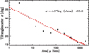 |
Fig. 1. Standard deviations of the observed tilt angle distributions binned in the logarithmic area. The error bars indicate one standard error estimates. The dashed line represents the fitting result given by Eq. (2). |
We use Eq. (1) in Sect. 3 to calculate σα, which is used for weighted fits to Joy’s law.
2.1.2. MW and KK data
Previous studies on tilt angles have depended heavily on the historical MW and KK4 data sets because they provide the longest available records of sunspot tilt angles. Both sets of data are based on white-light observations. The MW solar observatory has been conducting daily broadband observations of the entire disk since 1906. Images from 1917–1985 were measured using the method described by Howard et al. (1984) to determine the tilt angle of the sunspot group. The same measurement method was applied to the white-light images of KK to determine the tilt angle of the sunspot for the years 1906–1987.
We first follow what Dasi-Espuig et al. (2010) did to remove the invalid data by neglecting all zero tilt angles and the data that the distance between the leading and following portions is larger than 16°. We further neglect the data having zero leading or following polarity latitude and the data containing no spots in either portion of a group. Then we select the remaining MW and KK data within the ±60° CMD. Finally, we consider two cases of the selected data, namely, with or without the polarity separation filter  . There is no lifetime information in the two data sets because they did not keep track of any groups for more than two consecutive days. Hence, we cannot select the maximum phase of each sunspot group as we do in the case of the DPD data set. We consider the tilt angle of each group recorded on the first day. Since the three tilt angle data sets overlap from 1974 to 1985, we go on to choose the tilt angle data during this time period to compare their differences.
Table 4 shows the comparisons of the amount of data, the mean tilt angle,  , and standard deviation, σα among the four data sets (DPDmax, DPDall, KK, and MW). The amount of DPDall is about 6 times more than that of DPDmax. The amount of DPDmax is slightly less than that of KK and MW in the case of Δs ≥ 0° and is more than that of KK and MW in the case of
  . These result from that more sunspots with Δs < 2.5, most of which are regarded as the unipolar spots, are included in the KK and MW data sets. About 45% and 40% spots with Δs < 2.5 are included in KK and MW, respectively. In contrast, there are just 25% spots with Δs < 2.5 in DPD. This shows the superiority of the DPD data set and the importance to include the filter
  in KK and MW. We see a notable increase of
  with the filter of
  for the KK and MW data sets. In contrast,
  decreases for DPDmax with the filter
  . This might imply that for large sunspot groups, their tilt angles decrease before reaching their maximum area development. Another prominent property is that with the filter
  , the values of σα decrease, especially for the KK and MW data sets. As a whole, the DPD data are more stable and less affected by selection conditions by comparing with the KK and MW data sets. In comparing the KK and MW data, we see that
  for MW with
  is closer to the DPDall result than that for KK. The σα value for MW with
  (
( ) is smaller than that for KK (
 ). The σα value for DPDall (
 ) is the largest among the data sets with the filter
  . This is because that different evolution stages of big spots in DPDall provide extra contributions to the tilt scatter.
Comparisons among different data during 1974 to 1985.
2.2. Sunspot number data and sunspot area data
Two kinds of data, namely, 13-month smoothed monthly average total sunspot number5 and 13-month smoothed monthly averages of the daily sunspot areas6 (in units of millionths of a hemisphere, hereafter μHem.), were used to obtain the solar cycle strength. The latter contains the data for the full Sun and the separate northern and southern hemispheres. As shown in Fig. 2, the cycle amplitudes change obviously. The amplitude, indicated by both the sunspot number and area, is significantly weak in cycle 24. We use the maximum value of the 13-month averaged total area of sunspots as the cycle strength Sn for Sect. 3.4.1, where the separate hemispheres are considered. In the remaining part of the paper, we use the maximum value of the 13-month smoothed monthly average sunspot number as the cycle strength Sn.
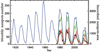 |
Fig. 2. Two kinds of solar cycle strength data. The blue curve shows the 13-month smoothed monthly sunspot number during cycles 15 to 24. The black (red) curve is the 13-month smoothed monthly averages of the daily sunspot areas in the northern (southern) hemisphere. And the total sunspot areas are represented by the green curve. |
At the beginning of a cycle, sunspots emerge at higher latitudes, while at lower latitudes some sunspots remain belonging to the previous cycle. Since there is an overlap of 2–4 yr between cycles, we take the time domain of one and a half years before and after the cycle minimum year as the cycle overlap. Data above a latitude threshold during the cycle overlap is allocated to the next cycle, and data below the latitude threshold is allocated to the previous cycle. Ultimately, our data is divided by solar cycles as shown in Fig. 3, and the data within each cycle is shown in different colors. We comment that some studies on the analysis of Joy’s law did not concern the separation of the two adjacent cycles during the overlap. This might give misleading results about the tilts near the equator and at high latitudes, especially the disputation of the tilt at the equator and the decrease of tilt at high latitudes (Tlatova et al. 2018).
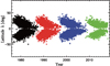 |
Fig. 3. Time-latitude diagram of sunspot groups based on DPDmax with individual cycles indicated by different colors. Cycles 21 to 24 are shown in black, red, blue, and green, respectively. |
3. Result
We first analyze the cycle-averaged tilt angle itself without removing the latitudinal dependence. Table 5 shows results based on DPD data for cycles 21–24 in the case of Δs ≥ 0°. The smallest and largest values of  are
are  (cycle 21) and
  (cycle 24), respectively. The difference between the two mean values of
  is only 0°.89. However, the uncertainty range of the mean, that is, standard error of the mean
  , is about half of it. The CC between
  and Sn is r = −0.83 (p = 0.10). We argue that this anti-correlation has no statistical significance whatever the CC is since
  is too large. We suggest a criterion to judge the statistical significance based on a parameter c, which is defined as follows:
 (3)
(3)
Tilt coefficients obtained by different methods based on DPD with Δs ≥ 0°.
where T represents the parameters listed in the second column of Table 5, while max(T) and min(T) are the maximum and minimum values of T for cycles 21–24, respectively, and max(σT) is the maximum standard error. We take c = 3.0 as the critical value. A larger c corresponds to a smaller σT, a larger difference of T among the investigated cycles, and hence a stronger statistical significance. If c is less than 3.0, we regard that there is no statistical significance. The smallest and largest values of  are
are  (cycle 21) and
  (cycle 24), respectively. Obviously,
  is much smaller than
  . This mainly results from about 6 times of data points in the case including all measurements. The corresponding c is 5.3. The CC between
  and Sn is r = −0.71 (p = 0.16).
Table 6 shows the same results as Table 5, but with the filter  . Both
  and
and  are smaller than those based on the cases without the filter. And the corresponding c-values are larger than those based on the cases without the filter. These show the importance to include the angular filter in the data selection so that the unipolar sunspot groups can be removed. Although the CC between
  and Sn is slightly increased compared with the case without the filter (−0.75 vs −0.71), the confidence level, 86%, is still lower than the widely accepted value, 95%. Tilt angles depend on latitudes. Stronger cycles tend to have sunspot emergence at higher latitudes, which show an opposite dependence on the solar cycle as the tilt angle does. Hence, we chose to investigate the tilt coefficients of different cycles, as suggested by Dasi-Espuig et al. (2010), and we discuss this in the following subsections.

3.1. Recovering Joy’s law
Different functions were used in previous studies to describe the increase of the tilt angle with increasing latitudes, namely, Joy’s law. The linear equation:
 (4)
(4)
is the most common to describe Joy’s law, where Tlin is the tilt coefficient corresponding to the linear function. Observations show that the trend of increasing tilt angle with latitude is saturated at high latitudes (Tlatov et al. 2013; Baranyi 2015). We refer to this phenomenon as high latitude saturation. A similar phenomenon has been found in numerical studies of sun-like stars for a range of rotation rates (Işık et al. 2018b). Hence Cameron et al. (2010), Jiang (2020) suggested the square-root function,
 (5)
(5)
describing Joy’s law, where Tsqr is the tilt coefficient corresponding to the square-root function. Both the linear and the square-root functions pass through the origin. There are also some studies (e.g., Wang & Sheeley 1991; Leighton 1969; Stenflo & Kosovichev 2012; Weber et al. 2012; Isik 2015; Jha et al. 2020; Yeates 2020) that use the sinusoidal function to fit Joy’s law. The sinusoidal function reflects the physical process if the origin of the systematic tilt is related to the Coriolis force since this force varies with latitude as sin λ. In the latitude belt where sunspots emerge frequently, the sinusoidal function is basically linear and almost identical to Eq. (4). Thus, we do not consider the sinusoidal form in this study. Furthermore, functions containing y-intercepts α0 have also been used (e.g., Wang & Sheeley 1991; Norton & Gilman 2005; Li & Ulrich 2012; Stenflo & Kosovichev 2012). Whether the average tilt angle at the equator is zero remains an open question (Kleeorin et al. 2020; Kuzanyan et al. 2019). Physically we prefer a zero tilt angle at the equator. And a cycle dependence of α0 also complicates the study. Hence, we do not consider functions containing y-intercepts in the study.
There are three major methods for obtaining the tilt coefficients, Tlin and Tsqr, of Joy’s law based on previous studies. We refer to the first one as the normalization method. Assuming the scatter in the tilt angles is random and unbiased, Dasi-Espuig et al. (2010), Cameron et al. (2010), Jiang (2020) calculate the normalized tilt coefficient  via:
via:
 (6)
(6)
and  via:
via:
 (7)
(7)
respectively. Here, Aj, λj and αj are the area, latitude, and tilt angle of the sunspot group j during a cycle, respectively. The area-weighted tilt angles are used to give more importance to the bigger sunspot groups, which have less tilt angle scatter.
The method used more widely is what we refer to as binned fitting method. The tilt angle data is grouped into bins by latitudes, and then the averages of the tilt angles in the latitude bins are fitted by the method of least squares. The method has been widely used to recover Joy’s law in many studies (e.g., McClintock & Norton 2013; Wang et al. 2014; Tlatov et al. 2013; Baranyi 2015). A valid and optimal choice for the number of bins is required. In most cases, 10 to 20 bins are the most predominant in practice (Cattaneo et al. 2019). However, people usually use bins of 5° latitudes, so that fewer than ten bins are used for curve fittings since most sunspot groups are within ±40°. A smaller bin width in latitudes brings more data points for linear or square-root fittings. But, simultaneously, a smaller bin width brings large errors in the average tilt angle of each bin because of less amount of sample points. Hence, there is the intrinsic problem with the method. Past studies have shown that even with the same data, different ways to deal with binning cause significantly different tilt coefficients, Tlin and Tsqr. McClintock & Norton (2013) even showed that for some cycles, Joy’s law appeared weak since they binned the tilt angle data of each cycle in 3° of latitude.
People usually perform a binned fit to data because the trend of the data can be better seen when the fitted form is unknown. But in the case that the function describing Joy’s law is already known, we can perform unbinned fits to the data so that no information is lost due to binning. We refer to the third method as the unbinned fitting method.
In the following, we calculate the tilt coefficients for cycles 21–24 using the above three methods based on DPDall and DPDmax, both with and without the filter,  . The results are presented in Table 5 (Δs ≥ 0°) and Table 6 (
 ). When we use the binned fitting method to obtain the tilt coefficients Tlin and Tsqr, we take into account that each fitted point has a different uncertainty, σα. We use 1/
 of each latitude bin as the weight. Figure 4 shows the tilt angles averaged over latitude bins versus latitude based on DPDall (left two panels) and based on DPDmax (right two panels) with Δs ≥ 0°. The tilt angles are separated by latitude bins in 5° except the last bin. The last bin contains data with latitudes greater than 30°, where there are relatively fewer sunspot records. The same method is adopted to analyze the data filtered by
  .
.
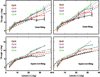 |
Fig. 4. Joy’s law obtained by the binned fitting method. The upper panels show the linear fitting and the lower panels show the square-root fitting. The left column is based on DPDall with Δs ≥ 0° and the right column is based on DPDmax with Δs ≥ 0°. Cycles 21 to 24 are shown in black, red, blue, and green, respectively. The dashed lines show the fitting result of the average values in 5° latitude bins by the least square method (the last bin contains data with latitudes greater than 30°). The error of the mean is the standard deviation of the bin sample divided by |

Figure 4 shows that there are differences between the two Joy’s law equations. In order to evaluate which one has a better fit to the data, we take into account the statistical parameter, χ2 as the goodness-of-fit. Table 5 shows that in the case of binned fitting method, χ2 varies from 7.30 (strong cycle 21) to 1.07 (weak cycle 24) for  , while χ2 varies from 1.74 (strong cycle 21) to 3.14 (weak cycle 24) for
  . The phenomena that the linear fits to the data of weaker cycles have smaller χ2-value and the square-root fits to the data of stronger cycles have smaller χ2-value are also presented by the DPDmax data and by the two data sets with the filter
  (Table 6). These indicate that the tilts tend to show a linear dependence on the latitudes for weak cycles and a square-root dependence for a strong cycle. In other words, the strong cycles tend to have the high latitude saturation of Joy’s law. Some studies have pointed out the high latitude saturation (e.g., Baranyi 2015; Tlatova et al. 2018; Nagovitsyn et al. 2021), but it seems that the cycle dependence of the saturation has not been pointed out based on our best knowledge.
A reason for the weak increase of the tilt angle at middle latitudes is the photospheric differential rotation, which has a strong effect at mid-latitudes and acts to decrease the tilts after the sunspot group emerges. The left and right panels of Fig. 4 corresponding to DPDall and DPDmax, respectively, show that DPDall have smaller tilt angles at middle latitudes than that of DPDmax. But still DPDmax for cycle 21 shows the square-root dependence on the latitudes. This might imply the saturation results from the flux emergence process. Previous efforts based on magnetograms gave different trends for cycle 21. Using tilt angles at each sunspot group maximum area development corresponding to the DPDmax data, Wang & Sheeley (1989) found a regular increase of the tilt angle with latitudes. Using tilt angles derived from daily magnetograms corresponding to the DPDall data, Howard (1989, 1991a) obtained a less regular increase at latitudes lower than 25° latitudes, and a strong decrease above that. A small bin size, 2.5°, could be a cause of the different latitude dependence.
For the unbinned fitting method, we also optimize the importance of the data by performing weighted fits. Sunspot groups with larger areas tend to have smaller uncertainties in tilts. We use Eq. (1) obtained in Sect. 2 to calculate each sunspot group’s tilt angle uncertainty σα. We add 1/ to each data point as a weight to increase the importance of the tilt angle data having smaller scatters. Figure 5 shows the dependence of the tilt angle on the unsigned latitude for the DPDmax data with
  . The same method is applied to deal with the DPDall data and the cases without the filter
  .
.
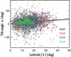 |
Fig. 5. Joy’s law obtained by the unbinned fitting method based on the DPDmax with |

The last 4 lines of Tables 5 and 6 show the results using the unbinned fitting method for the cases without and with the filter  , respectively. Like the results shown by the binned fitting method, square-root fitting to Joy’s law of stronger cycles tends to have smaller χ2-values. And linear fitting to Joy’s law of weaker cycles tend to have smaller χ2-values. But the difference of χ2-values between the strong and weak cycles is much smaller than that derived using the binned fitting method. For example, Table 5 shows that the χ2 values for the strong cycle 21 for
  and
and  are 1.15 and 1.09, respectively. The χ2 value for the weak cycle 24 for
  and
and  are 0.89 and 0.90, respectively.
In this subsection, we have described how to obtain the tilt coefficients with three methods and two Joy’s law equations. We have found that the tilts tend to show a linear dependence on the latitudes for weak cycles and a square-root dependence for strong cycles. In the next subsection, we analyze the cycle-to-cycle variations of the tilt coefficients and look for the relationship between the tilt coefficient and the cycle strength.
3.2. Cycle dependence of the tilt coefficient for cycles 21–24
The tilt coefficients of cycles 21–24 obtained by different methods are shown in Table 5 (Δs ≥ 0°) and Table 6 ( ). The CCs between the tilt coefficients and Sn along with the p-values are listed in the last 2 columns for different cases. They show varied CCs from r = −0.98 (p = 0.05) to r = −0.62 (p = 0.22) depending on the methods, similar to what we have presented in the introduction. Another prominent variation is the standard error of the tilt coefficient, σT, which results from the large uncertainty of the tilt. As Eq. (3) shown, the value of σT affects the statistical significance of the correlation.
Comparing the two sets of DPD, we see that the value of σT for DPDmax is almost twice that of DPDall. For  and
and  , typical values of σT for different methods are about 0.03 and 0.015, respectively. The results of
  are consistent with the last two lines of Table 1 of Wang et al. (2014), who also calculated the values. For a given cycle, but with the use of different methods to derive the tilt coefficients, the mean values of Tmax are similar to the mean values of Tall. According to the criterion of the statistical significance, namely, c ≥ 3.0, DPDmax data tend to have no statistical significance to analyze the correlation between the tilt coefficient and Sn. The large σT of DPDmax mainly results from the dramatic decline of the data amount from DPDall to DPDmax for a given cycle. Hence, although DPDmax corresponds to the clear evolution stages and without bias to large spots, the large uncertainties of the tilt coefficients lead to that it is inferior to DPDall to be used to investigate the correlation. We note that although σT of
  is large, it is still much smaller than the uncertainties of the tilt coefficients, which are roughly 0.05 based on Fig. 4 of Dasi-Espuig et al. (2010). This further demonstrates that the DPD data are more stable and have less ambiguous records than other data sets. In the following, we mainly investigate the tilt angle property based on DPDall for convenience. The cycle dependence of the sunspot group tilts at different evolution stages, including the maximum area development, will be investigated in our subsequent studies.
Comparing the three methods (normalization, binned, and unbinned fitting methods), we see that the normalization method has the largest σT and the unbinned fitting method has the smallest σT. For example, σT calculated by the three methods using DPDall for cycle 21 are 0.015, 0.012, and 0.01, respectively. This implies that the unbinned fitting method is effective in decreasing σT. To evaluate the linear fits and the square-root fits to Joy’s law, we compare their c-values. For each data set, the linear fit always has a larger c than that of the square-root fit. For example, in the case of the binned fitting method, the values of c for the linear fit and the square-root fit are 7.3 and 5.7, respectively. This indicates that, overall, the linear fit to Joy’s law is more effective in decreasing σT.
Comparing the results based on DPDall between Tables 5 and 6, we find that the average tilt coefficients in Table 6 are always larger than that in Table 5. The standard errors, σT, in Table 6 are always smaller than those in Table 5. The c-values are larger. These indicate that the filter  is also effective in minimizing the uncertainty by removing unipolar regions. Moreover, the increased tilt coefficient, that is, the slope of linear fit to Joy’s law is close to that measured based on magnetograms given by Wang et al. (2014). Wang et al. (2014) inferred systematic smaller tilts based on white-light images than that from magnetograms. This might result from the ambiguous data due to unipolar groups. Wang et al. (2014) suggest that although filtering out the unipolar groups brings the different data sets into better agreement with each other, the magnetic measurements still provide an upper bound on the tilt angles based on their Tables 1 and 2. Plage areas in the magnetograph measurements contribute to the remaining discrepancy, which was first pointed out by Howard (1996b).
We have shown that although it exists for all cases, the anti-correlation between the tilt coefficient and Sn has some uncertainty, which depends on the method analyzing the data. The method of linear unbinned fitting can minimize the uncertainty. To investigate the effects of different methods analyzing the tilt angle data on the results of the relationship, we present how we carried out the Monte Carlo experiments in the next subsection.
3.3. Evaluating different statistical methods with Monte Carlo experiments
In order to investigate how much the tilt scatter affects the relationship between the tilt coefficient and the cycle strength and to further evaluate which statistical method can minimize the uncertainty of the tilt coefficient, we employed the Monte Carlo simulations in the next step.
Our Monte Carlo experiments are based on the DPDall data with Δs ≥ 0°. The tilt angle of each sunspot group in the data set is artificially synthesized. Other parameters of each sunspot group are kept the same as their observed values. The major steps to synthesize the artificial tilt angles are as follows. We first assume that the tilt coefficient and the cycle strength are fully correlated. We consider both the linear and square-root Joy’s law equations. The corresponding tilt coefficients are Tlin and Tsqr, respectively. The relationships between the tilt coefficients and Sn are Tlin = −0.00067 * Sn + 0.53 and Tsqr = −0.0019 * Sn + 1.98, respectively. Please note that the two equations for the cycle dependence of the tilt coefficient are not the final ones we suggest. They are derived based on Table 5. Their profiles have no effects on the Monte Carlo results. Then we take the observed cycle amplitude, Sn, into these two equations. We obtain two sets of ideal tilt coefficients of each cycle for the linear and square-root forms of Joy’s law. Next we use the two sets of ideal tilt coefficients and the observed latitudes to obtain the ideal artificial tilt angles satisfying Joy’s law. Finally, we add random numbers to the ideal artificial tilt angle data. The artificial tilt angle of each sunspot group is derived as follows:
 (8)
(8)
 (9)
(9)
where N(0, 1) is a random number drawn from the Normal distribution, and σα is the standard deviation. We simulate the magnitude of tilt angle scatter by varying the range of σα. Observations show that the maximum scatter of tilt angles is within 30°. So we equably increase σα from 0° to 30° with 5° interval. We generate 10,000 sets of artificial tilt angles for each σα based on Eqs. (8) and (9).
We now analyze the effects of different tilt scatters on the CCs for different analysis methods based on the synthesized tilt angles data. The procedures are the same as those described in Sect. 3.1. The tilt coefficients are calculated using the three methods, namely: the normalization method, binned, and unbinned fitting methods, for both the linear and square-root Joy’s law equations. Then the new tilt coefficients are used to calculate the CCs, as described in Sect. 3.2. We average 10 000 sets of CCs calculated by artificial tilt angles for each σα. We plot the variations of the CCs with σα, shown in Fig. 6. The dashed curves are fitted functions of the relationships between tilt angle scatters σα and CCs. The equations of the curves are:
 (10)
(10)
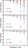 |
Fig. 6. Variations of the CCs with σα based on the Monte Carlo simulations. Panel a: results of the normalization method. Panel b: results of the binned fitting method. Panel c: results of the unbinned fitting method. The blue and red dotted curves depict the best-fit of the tilt angle scatter and correlation coefficients for the linear form and the square-root form of Joy’s law, respectively. Error bars represent one standard error for 10 000 correlation coefficients sets in each tilt angle scatters. |
where k is a constant for each data analysis method.
Figure 6 shows that the CC between the tilt coefficient and cycle strength decreases with increasing tilt angle scatter. When σα is 0°, the CCs are r = −1.0 for all cases. When σα is 30°, the mean CCs for the linear form of Joy’s law based on the three methods are −0.90, −0.97, and −0.97, respectively. The standard deviations of the CCs are 0.13, 0.02, and 0.02, respectively. These indicate that it is the large tilt scatter that causes the remarkably different CCs for different analysis methods. For the normalization method, around 95% of the CCs (2σα) for the 10 000 realizations in the case of σα = 30° are within the ranges from r = −0.64 to r = −1.0. When σα is equal to 30°, the mean CCs for the square-root form of Joy’s law based on the three methods are −0.80, −0.88, and −0.96, respectively. These values are all much lower than that for the linear form of Joy’s law. The standard deviations of CCs are 0.25, 0.19, and 0.08, respectively. They all are much larger than that for the linear form of Joy’s law. There is the possibility (about 0.3%, 3σα) that the CC is close to zero. The experiments demonstrate that the CCs obtained by the normalization method and square-root form of Joy’s law are strongly affected by the tilt angle scatter. And the CCs obtained by the unbinned fitting method and linear form of Joy’s law are less affected. We may conclude by the Monte Carlo experiments that the scatter of tilt angle leads to uncertainty in the CCs. The unbinned fitting method and linear form of Joy’s law can effectively minimize the effects of the uncertainty.
3.4. Extension of the data
3.4.1. Cycle dependence of the tilt coefficient for separate hemispheres of cycles 21–24
We have shown that in opting for a reasonable method to deal with the DPDall data during cycles 21–24, the CC between the tilt coefficient and cycle strength can reach −0.95. However, due to the fact that there are fewer sample points than in the case of the KK and MW data sets, the confidence level is 0.06. In order to further verify the anti-correlation, we increase the sample points by two approaches. This subsection describes the first one, separating the northern and southern hemispheres.
Previous studies have suggested that the tilt angle is asymmetric between the northern and southern hemispheres (Baranyi 2015; Işık et al. 2018a). Hale’s polarity law demonstrates the separate toroidal flux in the two hemispheres. The Coriolis force involved in the formation of the tilt angle depends on the local expansion rate of the rising flux tube and the local rotation rate. Hence, we consider that the tilt angles of the two hemispheres are independent and uncoupled. We use 13-month smoothed monthly averages of the daily sunspot areas to obtain the solar cycle strength, Sn since the sunspot number data for separate hemispheres is not directly available. We separate the data for the northern and southern hemispheres according to the positive and negative latitudes. We do not consider the normalization method to derive the tilt coefficients since it has been demonstrated that the method gives the largest uncertainty of the tilt coefficients. Furthermore, we only consider the results based on DPDall for the same reason.
The results are shown in Table 7. In comparing these results with those of Tables 5 and 6, we see that σT values tend to be slightly higher. This results from the decreased sample points for statistics. Although the σT-values are increased, c-values are larger than 3.0 for all cases. Values of σT based on the unbinned fitting method are prominently smaller than the corresponding values based on the binned fitting method. This adds another piece of evidence that the unbinned fitting method is advantageous when investigating the anti-correlation. We demonstrated in Sect. 3.1 that the tilts tend to show a linear dependence on the latitudes for weak cycles and a square-root dependence on strong cycles. This property exists for the separate hemispheres. We still take the strong cycle 21 and the weak cycle 24 as examples. For the linear form of Joy’s law and the fitting method to the binned Δs ≥ 0° data, the χ2 values for cycle 21 for the northern and southern hemispheres are 3.91 and 4.24, respectively. For the square-root form of Joy’s law, the corresponding χ2-values are 1.18 and 1.33, respectively. Each value is smaller than that from the linear form of Joy’s law. The strong cycle 22 shows the same property. In contrast, for the linear form of Joy’s law, the χ2 values for cycle 24 for the northern and southern hemispheres are 1.11 and 1.19, respectively. For the square-root form of Joy’s law, the corresponding χ2-values are 2.48 and 1.71, respectively. Each value is larger than the corresponding one from the linear form of Joy’s law. The weak cycle 23 shows the same property. Results from other methods, for instance, the unbinned fitting method and the data with  display the same property.
Tilt coefficients of each hemisphere obtained by fitting methods based on DPDall.
Table 7 shows that the tilt coefficient is strongly anti-correlated with the solar cycle strength. The CCs based on the unbinned fitting method are larger than those based on the binned fitting method. For example, for the data with the filter  , the CC is r = −0.76 at 97% confidence level in the case of the linear form of Joy’s law and binned fitting method. The corresponding CC is r = −0.81 at 98% confidence level for
  . The CCs based on the linear form of Joy’s law are larger than those based on the square-root form of Joy’s law. For example, for the data with the filter
  , the CC is r = −0.54 at 87% confidence level in the case of the square-root form of Joy’s law and the binned fitting method. The corresponding CC is r = −0.76 at 97% confidence level for the linear form of Joy’s law.
3.4.2. Combining DPD data with MW and KK data
In this subsection, we carry out the second approach to extend solar cycles by combining DPD data with MW and KK data. Both MW and KK data cover cycles 15 to 21. DPD data covers cycles 21 to 24. We have data covering ten solar cycles, which is advantageous when investigating the anti-correlation between the tilt coefficient and the cycle strength, if we can combine the two kinds of data sets. What we use here is the DPDall data.
Previous subsections have shown that the unbinned fitting method performs better with smaller calculation errors to get the tilt coefficient, so we adopt this method to deal with the MW and KK data. We still consider two cases of MW and KK data, which are with and without the polarity separation  . Both linear and square-root forms of Joy’s law are used to obtain the tilt coefficients. Because the area data of the sunspot group based on MW and KK is represented by only the umbra area of the group, we use Eq. (1) of Jiang et al. (2014a) to calculate σα, which are used for weighted fits to Joy’s law. Results for cycles 15 to 21 are shown in Table 8.
Tilt coefficients obtained by the unbinned fitting method based on MW and KK.
Compared with previous studies on KK and MW tilt angle analyses (e.g., Dasi-Espuig et al. 2010; Ivanov 2012), a prominent difference is concentrated on the uncertainty of each cycle’s tilt coefficient, σT. Our results are several times lower than those of previous studies, which is a benefit of the unbinned fitting method. For all cases, c-values are larger than 3.0. Hence, they all show statistical significance.
Comparing the results between Δs ≥ 0° and  , we see that the average tilt coefficients in the case of
  are much stronger, typically 30%, than that in the case of Δs ≥ 0°. The difference based on MW data is even larger than that based on KK data. Although Table 5 (DPD data with Δs ≥ 0°) shows smaller tilt coefficients than that from Table 6 (DPD data with
  ), the relative difference is smaller than that based on both KK and MW data sets. This implies that MW data could include more unipolar regions than the other two data sets. The DPD data has the best quality at least in identifying the two polarities of each sunspot group.
For the linear form of Joy’s law, the CCs are r = −0.65 (p = 0.08) and r = −0.84 (p = 0.03) based on the MW data without and with the filter of the angular separation, respectively. In contrast, for the square-root form of Joy’s law, the corresponding CCs are −0.54 (p = 0.15) and −0.79 (p = 0.04), respectively. The results based on the square-root form of Joy’s law show much weaker CCs. KK data presents the same property. This further implies that overall the linear form of Joy’s law better captures the property of sunspots’ latitudinal dependence.
The last column of Table 8 shows the ratios between the cycle 21 tilt coefficient derived based on different methods for the KK and MW data sets and the corresponding value based on DPDall. We designate the ratio as the factor, f. The f-values based on KK data in the cases of Δs ≥ 0° show large deviations from 1.0; namely, they are 1.27 and 1.39 for the linear and square-root forms of Joy’s law, respectively. The f values of other cases are close to 1.0. Especially for the linear form of Joy’s law based on MW data with  , the f value is 1.0, which means that our filter method and the unbinned fitting method are more reliable to study the relationship. Hence we combine MW data with
  with the corresponding DPDall data. We address that the filter
  has to be included to make the two data sets homogenous. Eq. (4) of Baranyi (2015) also gave the calibration factor between DPD and MW tilt data using the same selection criteria. The calibration factor is 1.01 ± 0.01, which is consistent with our result. The tilt coefficients of cycles 15 to 24 are calculated using the unbinned fitting method. The linear form of Joy’s law is adopted. The relationship between the tilt coefficients of cycles 15 to 24 and the corresponding cycle strength are shown in Fig. 7.
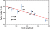 |
Fig. 7. Tilt coefficients based on the combined data versus the strength of cycles 15 to 24. The blue dots represent coefficients based on MW with |


The blue dots in Fig. 7 indicate the tilt coefficients calculated based on MW data. The black squares indicate the values calculated based on DPDall. The CC between the tilt coefficients Tlin for cycles 15 to 24 and the cycle strength Sn is r = −0.85 (p = 0.01). The red solid line indicates the least-square fit to their relationship. The linear fit between Tlin and Sn is shown in Eq. (11):
 (11)
(11)
For a given cycle, the tilt angles based on Eq. (11) are about 18% larger than those based on the results given by Dasi-Espuig et al. (2010), Jiang (2020). This is mainly because that the filter  was not included in the previous studies.
Figure 7 shows that except cycle 15, the weakest cycle 24 during cycles 15–24 has the largest tilt coefficient. The tilt coefficient of cycle 15 has a large uncertainty. This is due to the incomplete recording of MW data (the rising phase of cycle 15 is not recorded). The strongest cycle 19 during cycles 15–24 has the smallest tilt coefficient. Ivanov (2012) claimed that the abnormally strong cycle 19 contributed most to the anti-correlation. McClintock & Norton (2013) pointed out that southern hemispheric tilt angles for cycle 19 are responsible for the low mean tilt angles for the whole Sun in cycle 19. We investigate the number density distribution of cycles 15–21 for separate hemispheres. The southern hemisphere of cycle 19 shows a deviation from other hemispheric data of different cycles, which present a consistent number density distributions. The origin of the abnormal southern hemisphere of cycle 19 remains to be investigated. With the filter  , the deviation of cycle 19 tilt coefficient from the fitted line is much less than that shown by Ivanov (2012) and Dasi-Espuig et al. (2013). Aside from two controversial cycles (15 and 19), the tilt coefficients’ uncertainty of the remaining cycles is much smaller than that given by Ivanov (2012), Dasi-Espuig et al. (2013). The maximum σT given by us and by Dasi-Espuig et al. (2013) are 0.031 (cycle 16) and 0.37 (cycle 16, estimated based on their Fig. 1), respectively. For cycles 16–18 and 20–21, the difference between max(σT) and min(σT) is much larger than that given by Ivanov (2012), Dasi-Espuig et al. (2013), whose c values are less than 0.1. Our c value is 2.6. If we only remove cycles 15 and 19 from the 10 cycles, the c value is 3.2. The CC based on the remaining 8 cycles is r = −0.87 with p-value of 0.01. All these results show that our method is improved compared with previous ones, and there is clearly an anti-correlation between the tilt coefficient and the cycle strength with a significant confidence level. The improvements owe to the filter
  and the unbinned fitting method used in analyzing the data.
4. Conclusions and discussion
As remarked by van Driel-Gesztelyi & Green (2015), Joy’s law studies have been “studded with confusing and controversial results”. The dependence of Joy’s law on the solar cycle is a typical example. Our main objectives have been to pin down the causes of the controversial results and to find out the relationship between the tilt angles and the cycle strength. Besides the widely used historical MW and KK tilt angle data sets, we employed the more recent DPD data set for cycles 21–24. We have applied different filters to the data sets, for instance, with and without the angular separation,  , so that we can investigate the effects of filters on the properties of tilt angles. We also applied three previous main methods to analyze the data: the normalization method, binned fitting method, and unbinned fitting method. Furthermore, we assessd our results by utilizing Monte Carlo experiments. We summarize our main conclusions as follows.
-
The controversial statistics about the dependence of Joy’s law on the solar cycle result from the extremely wide scatter of tilt angles. Two factors contribute to the tilt angle scatter. One is due to the generation mechanism of the tilt angle which may involve the turbulent convection. The other is due to measurement errors. For example, some measurements have been carried out based on unipolar regions.
-
The filter, that is, the angular separation,
 is effective in removing the ambiguous measurements of unipolar regions. With the filter,
  , average tilt angles for different cycles based on the DPD, KK, or MW data sets are larger than that without the filter. They show consistent results with the tilt angles measured based on magnetograms. The corresponding standard deviations have a significant decrease, especially for KK and MW data.
 -
The tilts tend to show a linear dependence on the latitudes for weak cycles and a square-root dependence for strong cycles. In other words, the strong cycles tend to have the high latitude saturation of Joy’s law. The widely used linear Joy’s law equation shows the best fit to data of weaker cycles. The property is demonstrated by both the DPDall and DPDmax data. A square-root Joy’s law equation shows the best fit to data of stronger cycles. The mechanisms responsible for the latitudinal saturation are yet to be investigated.
-
The results based on the widely used binned fitting method are sensitive to the bins. Compared with the widely employed normalization method and the binned fitting method, the unbinned fitting method can minimize the effect of the tilt scatter on the uncertainty of the tilt coefficients. The result is supported by the Monte Carlo experiments.
-
The KK (∼45%) and MW (∼40%) data sets include more ambiguous measurement satisfying
 than the DPD data set (∼25%). The DPD data shows a good agreement with MW data during the overlapped cycle 21 after filtering out the
  measurements. The agreement during the two data sets provides the possibility to combine MW data for cycles 15–21 with DPD data for cycles 21–24.
 -
Based on the method generating the minimum uncertainty of the tilt coefficients, the tilt angle coefficients Tlin show an anti-correlation with the cycle strength Sn with a strong statistical significance (r = −0.85, p = 0.01) for cycles 15–24. The fitted relationship between Sn and Tlin follows Tlin = −0.00107 * Sn + 0.61. The DPD data for cycles 21–24 also shows a strong anti-correlation (r = −0.96). But the confidence level is slightly lower (p = 0.06) because of less sample data points. The separate hemispheric DPD data show a correlation coefficient as r = −0.84 (p = 0.02). The linear form of Joy’s law gives higher correlation coefficient than the square-root form of Joy’s law.
The confirmed anti-correlation between the tilt coefficient and the cycle strength provides a nonlinear mechanism to modulate the polar field generation for the variable amplitudes of solar cycles since the axial dipole moment contributed by each sunspot group is proportional to its tilt angle (Jiang et al. 2014b; Petrovay 2020). The polar field corresponds to the major component of the poloidal field in the framework of the BL-type dynamo (Cameron & Schüssler 2015). The generation of the toroidal field from the poloidal field is a quasi-linear process. Hence the anti-correlation works as a nonlinearity to modulate the solar cycle (Karak & Miesch 2017; Jiang 2020).
The cycle-dependent tilt angles have been included in surface flux transport simulations of Cameron et al. (2010), Jiang et al. (2011) to get the regular polar field reversals consistent with the observations. But the tilt coefficients used by these studies are based on the data without filtering out the unipolar regions. Tilt angles derived based on Eq. (11) are about 18% larger than what they used. The magnetic activity relevant inflows toward activity belts (Gizon & Rempel 2008; Cameron & Schüssler 2012) have been incorporated in these studies by a simplified factor g = 0.7 to mimic the effects of inflows on the tilts. With the larger tilt angles, stronger inflows are required to get the regular polar field reversals in surface flux transport models, which brings new constraints on the amplitudes of inflows.
Recent surface flux transport simulations assimilated the realistic magnetic configuration of sunspot groups as the flux sources into their models (e.g., Wang et al. 2020; Yeates 2020). Some sunspot groups with complex configurations usually give strikingly different contributions to the polar field compared with the BMR approximations (Jiang et al. 2019; Yeates 2020; Wang et al. 2020). Wang et al. (2021) recently proposed a generalized algebraic method to quickly predict the axial dipole contribution of a sunspot group with an arbitrary configuration. The complex configurations of sunspot groups are beyond the description of tilt angles. Although there has been recent progress in improving the understanding of the importance of the realistic configurations on the polar field evolution, we argue that it is still essential to investigate the statistical properties of tilt angles, especially their cycle dependence. Most spots and most cycles obey the statistical properties, namely, Joy’s law and the cycle dependence of tilt coefficients. Investigations of tilt angles help to identify the randomness mechanism of the solar cycle and to understand the flux tube emergence. The statistical properties are helpful in the reconstruction of the long-term behavior of the solar magnetic field.
As a sunspot group evolves over the solar surface, its tilt angle varies with time. The properties at different evolutionary stages help us understand the physical origin of tilt angles. The DPD data continuously recorded the each sunspot group every day. The data sets enable studies on tilt angle evolution. In this work, we have carried out simple investigations on the maximum phase of each sunspot group. We will address the evolutionary processes in a subsequent study.
Acknowledgments
We thank the referee for the valuable comments and suggestions on improving the manuscript. This research was supported by the National Natural Science Foundation of China through grant Nos. 11873023 and 11522325, the Fundamental Research Funds for the Central Universities of China, Key Research Program of Frontier Sciences of CAS through grant No. ZDBS-LY-SLH013, the B-type Strategic Priority Program of CAS through grant No. XDB41000000. JJ acknowledges the International Space Science Institute Teams 474 and 475.
References
- Babcock, H. W. 1961, ApJ, 133, 572 [Google Scholar]
- Baranyi, T. 2015, MNRAS, 447, 1857 [NASA ADS] [CrossRef] [Google Scholar]
- Baranyi, T., Gyori, L., & Ludmány, A. 2016, Sol. Phys., 291, 3081 [NASA ADS] [CrossRef] [Google Scholar]
- Caligari, P., Moreno-Insertis, F., & Schussler, M. 1995, ApJ, 441, 886 [Google Scholar]
- Cameron, R. H., & Schüssler, M. 2012, A&A, 548, A57 [NASA ADS] [CrossRef] [EDP Sciences] [Google Scholar]
- Cameron, R., & Schüssler, M. 2015, Science, 347, 1333 [NASA ADS] [CrossRef] [Google Scholar]
- Cameron, R. H., Jiang, J., Schmitt, D., & Schüssler, M. 2010, ApJ, 719, 264 [NASA ADS] [CrossRef] [Google Scholar]
- Cattaneo, M. D., Crump, R. K., Farrell, M., & Feng, Y. 2019, FRB of New York Staff Report, No. 881 [Google Scholar]
- Dasi-Espuig, M., Solanki, S. K., Krivova, N. A., Cameron, R., & Peñuela, T. 2010, A&A, 518, A7 [NASA ADS] [CrossRef] [EDP Sciences] [Google Scholar]
- Dasi-Espuig, M., Solanki, S. K., Krivova, N. A., Cameron, R., & Peñuela, T. 2013, A&A, 556, C3 [NASA ADS] [CrossRef] [EDP Sciences] [Google Scholar]
- D’Silva, S., & Howard, R. F. 1993, Sol. Phys., 148, 1 [NASA ADS] [CrossRef] [Google Scholar]
- Fisher, G. H., Fan, Y., & Howard, R. F. 1995, ApJ, 438, 463 [NASA ADS] [CrossRef] [Google Scholar]
- Gizon, L., & Rempel, M. 2008, Sol. Phys., 251, 241 [NASA ADS] [CrossRef] [Google Scholar]
- Győri, L., Baranyi, T., & Ludmány, A. 2011, in Physics of Sun and Star Spots, eds. D. Prasad Choudhary, & K. G. Strassmeier, 273, 403 [Google Scholar]
- Gyori, L., Ludmány, A., & Baranyi, T. 2016, MNRAS, 465, 1259 [Google Scholar]
- Hale, G. E., Ellerman, F., Nicholson, S. B., & Joy, A. H. 1919, ApJ, 49, 153 [NASA ADS] [CrossRef] [Google Scholar]
- Howard, R. F. 1989, Sol. Phys., 123, 271 [NASA ADS] [CrossRef] [Google Scholar]
- Howard, R. F. 1991a, Sol. Phys., 132, 49 [NASA ADS] [CrossRef] [Google Scholar]
- Howard, R. F. 1991b, Sol. Phys., 136, 251 [NASA ADS] [CrossRef] [Google Scholar]
- Howard, R. F. 1993, Sol. Phys., 145, 105 [NASA ADS] [CrossRef] [Google Scholar]
- Howard, R. F. 1996a, Sol. Phys., 167, 95 [CrossRef] [Google Scholar]
- Howard, R. F. 1996b, Sol. Phys., 169, 293 [NASA ADS] [Google Scholar]
- Howard, R., Gilman, P. I., & Gilman, P. A. 1984, ApJ, 283, 373 [NASA ADS] [CrossRef] [Google Scholar]
- Işık, E., Işık, S., & Kabasakal, B. B. 2018a, Proc. Int. Astron. Union, 13, 133 [Google Scholar]
- Işık, E., Solanki, S. K., Krivova, N. A., & Shapiro, A. I. 2018b, A&A, 620, A177 [NASA ADS] [CrossRef] [EDP Sciences] [Google Scholar]
- Isik, E. 2015, ApJ, 813, L13 [NASA ADS] [CrossRef] [Google Scholar]
- Ivanov, V. G. 2012, Geomag. Aeron., 52, 999 [NASA ADS] [CrossRef] [Google Scholar]
- Jha, B. K., Karak, B. B., Mandal, S., & Banerjee, D. 2020, ApJ, 889, L19 [NASA ADS] [CrossRef] [Google Scholar]
- Jiang, J. 2020, ApJ, 900, 19 [Google Scholar]
- Jiang, J., Cameron, R. H., Schmitt, D., & Schüssler, M. 2011, A&A, 528, A83 [NASA ADS] [CrossRef] [EDP Sciences] [Google Scholar]
- Jiang, J., Cameron, R. H., & Schüssler, M. 2014a, ApJ, 791, 5 [Google Scholar]
- Jiang, J., Hathaway, D. H., Cameron, R. H., et al. 2014b, Space Sci. Rev., 186, 491 [Google Scholar]
- Jiang, J., Song, Q., Wang, J.-X., & Baranyi, T. 2019, ApJ, 871, 16 [Google Scholar]
- Karak, B. B., & Miesch, M. 2017, ApJ, 847, 69 [NASA ADS] [CrossRef] [Google Scholar]
- Kitchatinov, L. L., & Olemskoy, S. V. 2011, Astron. Lett., 37, 656 [NASA ADS] [CrossRef] [Google Scholar]
- Kleeorin, N., Safiullin, N., Kuzanyan, K., et al. 2020, MNRAS, 495, 238 [NASA ADS] [CrossRef] [Google Scholar]
- Kosovichev, A. G., & Stenflo, J. O. 2008, ApJ, 688, L115 [NASA ADS] [CrossRef] [Google Scholar]
- Kuzanyan, K. M., Safiullin, N., Kleeorin, N., Rogachevskii, I., & Porshnev, S. 2019, Astrophysics, 62, 261 [CrossRef] [Google Scholar]
- Leighton, R. B. 1969, ApJ, 156, 1 [Google Scholar]
- Lemerle, A., & Charbonneau, P. 2017, ApJ, 834, 133 [NASA ADS] [CrossRef] [Google Scholar]
- Li, D. 2017, Res. Astron. Astrophys., 17, 040 [Google Scholar]
- Li, J. 2018, ApJ, 867, 89 [CrossRef] [Google Scholar]
- Li, J., & Ulrich, R. K. 2012, ApJ, 758, 115 [NASA ADS] [CrossRef] [Google Scholar]
- Longcope, D. W., Fisher, G. H., & Arendt, S. 1996, ApJ, 464, 999 [NASA ADS] [CrossRef] [Google Scholar]
- McClintock, B. H., & Norton, A. A. 2013, Sol. Phys., 287, 215 [NASA ADS] [CrossRef] [Google Scholar]
- Nagovitsyn, Y. A., Osipova, A. A., & Pevtsov, A. A. 2021, MNRAS, 501, 2782 [NASA ADS] [CrossRef] [Google Scholar]
- Norton, A. A., & Gilman, P. A. 2005, ApJ, 630, 1194 [NASA ADS] [CrossRef] [Google Scholar]
- Petrovay, K. 2020, Liv. Rev. Sol. Phys., 17, 2 [Google Scholar]
- Schrijver, C. J., De Rosa, M. L., & Title, A. M. 2002, ApJ, 577, 1006 [Google Scholar]
- Schunker, H., Baumgartner, C., Birch, A. C., et al. 2020, A&A, 640, A116 [NASA ADS] [CrossRef] [EDP Sciences] [Google Scholar]
- Senthamizh Pavai, V., Arlt, R., Dasi-Espuig, M., Krivova, N. A., & Solanki, S. K. 2015, A&A, 584, A73 [NASA ADS] [CrossRef] [EDP Sciences] [Google Scholar]
- Senthamizh Pavai, V., Arlt, R., Diercke, A., Denker, C., & Vaquero, J. 2016, Adv. Space Res., 58, 1468 [NASA ADS] [CrossRef] [Google Scholar]
- Sivaraman, K. R., Gupta, S. S., & Howard, R. F. 1999, Sol. Phys., 189, 69 [NASA ADS] [CrossRef] [Google Scholar]
- Solanki, S. K., Wenzler, T., & Schmitt, D. 2008, A&A, 483, 623 [NASA ADS] [CrossRef] [EDP Sciences] [Google Scholar]
- Stenflo, J. O., & Kosovichev, A. G. 2012, ApJ, 745, 129 [NASA ADS] [CrossRef] [Google Scholar]
- Tlatov, A., Illarionov, E., Sokoloff, D., & Pipin, V. 2013, MNRAS, 432, 2975 [NASA ADS] [CrossRef] [Google Scholar]
- Tlatova, K., Tlatov, A., Pevtsov, A., et al. 2018, Sol. Phys., 293, 118 [NASA ADS] [CrossRef] [Google Scholar]
- van Driel-Gesztelyi, L., & Green, L. M. 2015, Liv. Rev. Sol. Phys., 12, 1 [NASA ADS] [CrossRef] [Google Scholar]
- Wang, Y. M., & Sheeley, N R., Jr. 1991, ApJ, 375, 761 [NASA ADS] [CrossRef] [Google Scholar]
- Wang, Y. M., Sheeley, N. R., Jr. 1989, Sol. Phys., 124, 81 [NASA ADS] [CrossRef] [Google Scholar]
- Wang, Y.-M., Colaninno, R. C., Baranyi, T., & Li, J. 2014, ApJ, 798, 50 [NASA ADS] [CrossRef] [Google Scholar]
- Wang, Z.-F., Jiang, J., Zhang, J., & Wang, J.-X. 2020, ApJ, 904, 62 [Google Scholar]
- Wang, Z.-F., Jiang, J., & Wang, J.-X. 2021, A&A, 650, A87 [NASA ADS] [CrossRef] [EDP Sciences] [Google Scholar]
- Weber, M. A., Fan, Y., & Miesch, M. S. 2012, Sol. Phys., 287, 239 [Google Scholar]
- Yeates, A. R. 2020, Sol. Phys., 295, 1 [Google Scholar]
All Tables
Summary of the controversial statistics on the cycle dependence of the tilt coefficient.
Tilt coefficients of each hemisphere obtained by fitting methods based on DPDall.
All Figures
|
Fig. 1. Standard deviations of the observed tilt angle distributions binned in the logarithmic area. The error bars indicate one standard error estimates. The dashed line represents the fitting result given by Eq. (2). |
| In the text | |
|
Fig. 2. Two kinds of solar cycle strength data. The blue curve shows the 13-month smoothed monthly sunspot number during cycles 15 to 24. The black (red) curve is the 13-month smoothed monthly averages of the daily sunspot areas in the northern (southern) hemisphere. And the total sunspot areas are represented by the green curve. |
| In the text | |
|
Fig. 3. Time-latitude diagram of sunspot groups based on DPDmax with individual cycles indicated by different colors. Cycles 21 to 24 are shown in black, red, blue, and green, respectively. |
| In the text | |
|
Fig. 4. Joy’s law obtained by the binned fitting method. The upper panels show the linear fitting and the lower panels show the square-root fitting. The left column is based on DPDall with Δs ≥ 0° and the right column is based on DPDmax with Δs ≥ 0°. Cycles 21 to 24 are shown in black, red, blue, and green, respectively. The dashed lines show the fitting result of the average values in 5° latitude bins by the least square method (the last bin contains data with latitudes greater than 30°). The error of the mean is the standard deviation of the bin sample divided by |
| In the text | |
|
Fig. 5. Joy’s law obtained by the unbinned fitting method based on the DPDmax with |
| In the text | |
|
Fig. 6. Variations of the CCs with σα based on the Monte Carlo simulations. Panel a: results of the normalization method. Panel b: results of the binned fitting method. Panel c: results of the unbinned fitting method. The blue and red dotted curves depict the best-fit of the tilt angle scatter and correlation coefficients for the linear form and the square-root form of Joy’s law, respectively. Error bars represent one standard error for 10 000 correlation coefficients sets in each tilt angle scatters. |
| In the text | |
|
Fig. 7. Tilt coefficients based on the combined data versus the strength of cycles 15 to 24. The blue dots represent coefficients based on MW with |
| In the text | |
Current usage metrics show cumulative count of Article Views (full-text article views including HTML views, PDF and ePub downloads, according to the available data) and Abstracts Views on Vision4Press platform.
Data correspond to usage on the plateform after 2015. The current usage metrics is available 48-96 hours after online publication and is updated daily on week days.
Initial download of the metrics may take a while.