| Issue |
A&A
Volume 653, September 2021
|
|
|---|---|---|
| Article Number | A102 | |
| Number of page(s) | 14 | |
| Section | Interstellar and circumstellar matter | |
| DOI | https://doi.org/10.1051/0004-6361/202140670 | |
| Published online | 14 September 2021 | |
The ionization fraction in OMC-2 and OMC-3
1
Green Bank Observatory,
155 Observatory Road,
Green Bank,
WV
24915,
USA
e-mail: This email address is being protected from spambots. You need JavaScript enabled to view it.
2
Max-Planck-Institut fur Radioastronomie,
Auf dem Hügel 69,
53121
Bonn,
Germany
3
National Radio Astronomy Observatory,
520 Edgemont Road,
Charlottesville,
VA
22903,
USA
4
Haystack Observatory, Massachusetts Institute of Technology,
Westford,
MA
01886,
USA
5
Leiden Observatory, Leiden University,
PO Box 9513,
2300
RA
Leiden,
The Netherlands
Received:
26
February
2021
Accepted:
24
June
2021
Abstract
Context. The electron density (ne−) plays an important role in setting the chemistry and physics of the interstellar medium. However, measurements of ne− in neutral clouds have been directly obtained only toward a few lines of sight or they rely on indirect determinations.
Aims. We use carbon radio recombination lines and the far-infrared lines of C+ to directly measure ne− and the gas temperature in the envelope of the integral shaped filament (ISF) in the Orion A molecular cloud.
Methods. We observed the C102α (6109.901 MHz) and C109α (5011.420 MHz) carbon radio recombination lines (CRRLs) using the Effelsberg 100 m telescope at ≈2′ resolution toward five positions in OMC-2 and OMC-3. Since the CRRLs have similar line properties, we averaged them to increase the signal-to-noise ratio of the spectra. We compared the intensities of the averaged CRRLs, and the 158 μm-[CII] and [13CII] lines to the predictions of a homogeneous model for the C+/C interface in the envelope of a molecular cloud and from this comparison we determined the electron density, temperature and C+ column density of the gas.
Results. We detect the CRRLs toward four positions, where their velocity (vLSR ≈ 11 km s−1) and widths (σv ≈ 1 km s−1) confirms that they trace the envelope of the ISF. Toward two positions we detect the CRRLs, and the 158 μm-[CII] and [13CII] lines with a signal-to-noise ratio ≥5, and we find ne− = 0.65 ± 0.12 cm−3 and 0.95 ± 0.02 cm−3, which corresponds to a gas density nH ≈ 5 × 103 cm−3 and a thermal pressure of pth ≈ 4 × 10⁵ K cm−3. We also constrained the ionization fraction in the denser portions of the molecular cloud using the HCN(1–0) and C2H(1–0) lines to x(e−) ≤ 3 × 10⁻⁶.
Conclusions. The derived electron densities and ionization fraction imply that x(e−) drops by a factor ≥100 between the C+ layer and the regions probed by HCN(1–0). This suggests that electron collisional excitation does not play a significant role in setting the excitation of HCN(1–0) toward the region studied, as it is responsible for only ≈10% of the observed emission.
Key words: ISM: lines and bands / radio lines: ISM / ISM: clouds
© ESO 2021
1 Introduction
The electrondensity,  , plays a fundamental role in the physics, chemistry, and dynamics of the neutral (atomic or molecular) interstellar medium (ISM). Collisions with electrons ejected through the photo-ionization of polyciclic aromatic hydrocarbons (PAHs) and small dust grains provide the main heating mechanism in regions exposed to far-ultraviolet (FUV) photons with energies < 13.6 eV (e.g., Watson 1972; Hollenbach & Tielens 1999). The electron density also determines the rate of fast ion-neutral reactions in molecular clouds, one of the main channels for the build-up of molecular complexity (e.g., Herbst & Klemperer 1973; Oppenheimer & Dalgarno 1974). In addition, the abundance of electrons relative to the neutrals, the ionization fraction (
 ), mediates the coupling between neutral gas and magnetic fields through ion-neutral friction (e.g., Mestel & Spitzer 1956). Finally, large dipole moment molecules, such as HCN and CN, have large inelastic collision cross sections with electrons, which leads to the significant rotational excitation of these molecules in regions where x(e−) ≥ 10−5 (e.g., Dickinson et al. 1977; Black & van Dishoeck 1991; Goldsmith & Kauffmann 2017).
The regions of the neutral ISM where FUV photons regulate the heating and chemistry are known as photodissociation regions (PDRs). In the outer layers of PDRs, the gas is neutral and carbon is singly ionized since it has a lower ionization potential than hydrogen (11.2 eV). This makes carbon one of the main donors of free electrons in the outer layers of PDRs. As we move deeper into a PDR, away from the source of FUV photons, the number of FUV photons drops and C+ recombines with free electrons in the C+/C interface. After recombination, carbon can be found in a highly excited electronic state as a Rydberg atom, and while the electron cascades to the ground energy levels it will emit at radio frequencies. The lines observed from this cascade are known as carbon radio recombination lines (CRRLs, Gordon & Sorochenko 2009), and along with the far-infrared line of C+ at 158 μm, [CII], they are important tracers of PDRs. Since the intensities of [CII] and CRRLs have different dependencies on the gas temperatureand density, their combined use is a powerful probe of the gas properties in a PDR (e.g., Natta et al. 1994; Sorochenko & Tsivilev 2010; Tsivilev 2014; Salgado et al. 2017b; Cuadrado et al. 2019; Salas et al. 2019; Siddiqui et al. 2020), such as the envelopes of molecular clouds.
Deeper into the PDR, past the C+/C interface, most of the carbon is in the form of CO and the electron density is mainly set by cosmic-ray ionization. In the dense cores of molecular clouds, the cosmic ray ionization rate (CRIR) is typically ~ 10−17 s−1 (Caselli et al. 1998; van der Tak & van Dishoeck 2000), leading to x(e−)~10−9–10−6 (e.g., Caselli et al. 1998; Goicoechea et al. 2009). In a stationary, onion-like, view of molecular clouds it is in these dense cores that the abundances of molecules are high enough for their emission to be detected. However, porosity of the PDR to FUV radiation might leave the cold clouds exposed to FUV radiation. Measuring the ionization fraction at different depths in a PDR provides insight into the structure of PDRs, the penetration of FUV radiation and the excitation of molecules with large dipole moments, for example, HCN.
Due to its high optically thin critical density (~ 105 cm−3, e.g., Shirley 2015), HCN(1–0) has been used as a tracer of dense molecular gas ( cm−3, e.g., Gao & Solomon 2004). However, recent studies of molecular clouds in our Galaxy show that a large fraction of the HCN(1–0) emission traces regions where the gas density is ~ 103 cm−3 (e.g., Kauffmann et al. 2017; Pety et al. 2017). Since the gas density is an essential parameter in our theories of star formation (e.g., McKee & Ostriker 2007), it is important to determine the characteristic density of the gas traced by HCN, and what processes dominate the excitation of HCN(1–0) at different densities. Some of the mechanisms responsible for the HCN(1–0) emission at low densities include additional collisional excitation of the transition due to collisions with electrons in high ionization fraction regions (e.g., Dickinson et al. 1977; Black & van Dishoeck 1991; Goldsmith & Kauffmann 2017), an elevated gas temperature due to cosmic ray heating (e.g., Meijerink et al. 2011; Vollmer et al. 2017) and radiative trapping due to a large line optical depth (e.g., Evans 1999; Shirley 2015). To assess the importance of these mechanisms it is necessary to obtain independent constraints on the gas properties, such as its temperature and density.
At a distance of 414 pc (Menten et al. 2007; Zari et al. 2017) Orion A is the closest molecular cloud where massive stars have recently formed. In the northern most portion of Orion A, Bally et al. (1987) identified an integral shaped filament (ISF) ~ 13 pc long. The northern half of the ISF is composed of OMC-2 and OMC-3 (Gatley et al. 1974; Morris et al. 1974). Their masses, as inferred from C18 O observations, are 113 M⊙ and 140 M⊙, respectively(Dutrey et al. 1993), and they cover an area ≈ 2.5 × 2.5 pc2. The mild radiation field and the presence of embedded stars (e.g., Megeath et al. 2012) make OMC-2 and OMC-3 representative of an average star forming molecular cloud in the Milky Way. It is also toward these clouds that Kauffmann et al. (2017) studied HCN(1–0) emission, and by modeling the ISF as a cylinder with a diameter of 2 pc they conclude that 50% of the HCN(1–0) emission traces regions with densities below ~ 103 cm−3.
In this work we target five regions toward OMC-2/3 to study how the ionization fraction changes from the envelope of the molecular cloud to its denser core. We use CRRLs and [CII] to measure the temperature and electron density of the molecular cloud’s envelope, and we use observations of molecular gas tracers (i.e., HCN and C2 H) to constrainthe ionization fractions deeper into the cloud. We use these constraints on x(e−) to determine the role of collisions with electrons in the excitation of the HCN(1–0) line. When quoting uncertainties we give the 1σ ranges unless otherwise noted.
2 Observations
2.1 5 GHz RRLs
We observed the n = 110, 109 and 102 α1 CRRLs at 4876.588, 5011.420 and 6109.901 MHz, respectively, with the Effelsberg 100m radio telescope during 2019 December and 2020 March. We used the wide-band Effelsberg C-band receiver (S45mm) at the secondary focus, which uses linear polarization feeds. The spectra were recorded with fast Fourier transform spectrometer backends (Klein et al. 2012). They provide two 200 MHz-wide bands with 65 536 channels each and a channel width of 38.1 kHz. We place these at 4941.0 MHz to capture the n = 110 and 109 α CRRLs, and at 6111.0 MHzfor the n = 102α CRRL. A summary of the radio recombination lines (RRLs) covered by the spectral setup is presented in Table 1.
We targeted five regions, shown in Fig. 1 and presented in Table 2. The observationswere done in position switching, with the reference position listed as “OFF” in Table 2. As flux calibrator we observed NGC 7027 (2105+420, Ott et al. 1994) at the beginning of each session. The pointing was checked regularly on 3C161 or 0420-014, with a typical pointing accuracy of ≲5′′. We also observed M42 as a reference before each observation.
The observations were reduced with the Effelsberg reduction pipeline, based on standard single-dish techniques as described in Kraus (2009). We reduced each 200-MHz-wide band separately, and verified that frequency-dependent effects of the bandpass, system temperature and the noise diode (Winkel et al. 2012) were marginal (≲ 3%) in our setup. The pipeline used the new water vapor radiometer for atmospheric opacity correction (Roy et al. 2004). The native channel width is 0.15 km s−1 and 0.18 km s−1 at 6111 MHz and 4941 MHz, respectively. Due to gridding of the spectra to the Kinematic Local Standard of Rest (LSRK) frame (Reid et al. 2009) in the reduction process the final spectral resolution is degraded by a factor of two with respect to the native channel width. The absolute flux calibration was done by comparing pointing observations with a flux density model of NGC 7027 which is based on regular Effelsberg monitoring (Kraus et al., priv. comm.). Typical system temperatures during the observations were ≈ 50 K. The beam sizes are 114′′ and 138′′, the sensitivity in K Jy−1 is 1.63 and 1.66 and the main beam efficiency is 0.65 and 0.64 for the bands at 6111 MHz and 4941 MHz, respectively, which were used to convert the observed antenna temperatures to main beam temperatures. The absolute flux calibration is accurate to 10–20%.
Once the spectra have been calibrated we average the C109α and C102α lines (rest frequencies 5011.422 and 6109.902 MHz, respectively2), after bringing them to the same velocity grid with a channel size of 0.18 km s−1 and a velocity resolution of ~ 0.36 km s−1. The C110α line is contaminated by radio frequency interference, so we do not include it. The averaged spectra have a mean frequency of 5557.9 MHz, which lies between that of the C106α and C105α lines. In the following we adopt a frequency of 5446.976 MHz, which corresponds to a transition with a principal quantum number n = 106, and a beam size of 126′′ for the averaged CRRL spectra.
The data contain additional ripples at very low intensity (< 0.50 mK peak-to-trough variations). The ripples are of sinusoidal shape with typical frequencies of 5.8 MHz (~ 300 km s−1 at the observed frequencies). Since they are much broader than then narrow CRRLs (~ 1 km s−1, e.g., Cuadrado et al. 2019), we remove a 1st order polynomial baseline around the expected velocity of the CRRLs. To recover information on the detection of hydrogen radio recombination lines (HRRLs), which are broader (~ 20–30 km s−1, e.g., Luisi et al. 2019), we model the baseline on a scan-by-scan basis by fitting a sinus function over at least three periods. Further baselines are removed after stacking. We compare this to interpolating the 5.8 MHz frequency of the baseline in Fourier space. The HRRLs toward EFF1 and EFF2 are detected in both methods. EFF4 is detected marginally after smoothing and stacking with a signal-to-noise ratio (S/N) of 5. We do not report detections for EFF3 and EFF5, since EFF3 is not detected when removing the baseline in Fourier space, and EFF5 is detected in neither method.
 |
Fig. 1 Location of the Effelsberg 5 GHz RRL observations presented in this work. Left: map of the peak temperature of the [CII] line over a one square degree centered on the Trapezium stars (Pabst et al. 2019). A green rectangle shows the extent of the region displayed on the right. Right: Spitzer IRAC 8 μm image of the OMC-2/3. The regions observed in 5 GHz RRLs are marked with solid black circles 1.′89 in diameter, while the dashed gray circles show the C76α observationsof Kutner et al. (1985) at 2′ resolution. The small green circles show the location of the sources detected in 3.6 cm radio continuum (Reipurth et al. 1999). |
Spectral setup of the C-band observations with the Effelsberg 100 m radio telescope.
Regions observed with the Effelsberg 100 m radio telescope.
2.2 Literature data
2.2.1 FIR C+
We use the 158 μm-[CII] line cube presented by Pabst et al. (2019). This data cube resulted from observations with the upGREAT receiver (Heyminck et al. 2012; Risacher et al. 2016) onboard the Stratospheric Observatory for Infrared Astronomy (SOFIA, Young et al. 2012). The [CII] cube has a spatial resolution of 16′′ and a velocity resolution of 0.2 km s−1, and covers a region of roughly 1° × 1°. To compare the FIR cube to the radio observations we convolve it to a spatial resolution of 126′′.
2.2.2 Dust
To determine the dust conditions toward the regions observed in RRLs we use the temperature and opacity maps of Lombardi et al. (2014). These maps constructed by combining FIR data obtained with Herschel and Planck and provide the dust properties at a resolution of 36′′. We use the dust opacity as a proxy for the column density of the neutral gas, N(H) = N(H2 + HI). To convert from optical depth to extinction at K band we adopt their conversion AK = 2640τ850 mag, a ratio AK∕AV = 0.112 and N(H)∕AV = 2.07 × 1021 cm−2 mag−1. Additionally, we use the dust temperature to estimate G0, the FUV radiation field at the surface of the PDR in Habing units (1.6 × 10⁻³ erg s−1 cm−2, Habing 1968), from  K (Hollenbach et al. 1991).
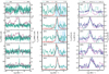 |
Fig. 2 CRRL spectra observed toward the northern part of the ISF with the Effelsberg 100 m radio telescope. The CRRL is an average of the C109α and C102α lines. We compare the averaged CRRL to the averaged HRRL (an average of the H109α and H102α lines, on the left), the FIR [CII] and [13CII] F = 2– 1 lines (center), and HCN(1–0) and C2 H(1–0) (right). In the center panels the [13CII] F = 2– 1 line is scaledto match the peak of the averaged CRRL, while on the right panels the CRRL is scaled to match the peak of the HCN(1–0) line. |
2.2.3 Molecular gas
As a measure of the column density of molecular hydrogen we use the N(H2) map of Berné et al. (2014) derived from the 12CO(2–1) and 13CO(2–1) lines at ≈11′′. For the temperature and line widths of the dense molecular gas we use the NH3 data cubes produced as part of the Green Bank Ammonia Survey (GAS) data release 1 (Friesen et al. 2017). We rederive the line properties and gas temperature at the spatial resolution of the CRRL observations using pySpecKit (Ginsburg & Mirocha 2011). We also use the HCN(1–0) and C2 H(1–0) (J = 1∕2–1∕2) data cubes of Melnick et al. (2011), as their ratio can be used as a probe of x(e−) (Bron et al. 2021). The C2 H(1–0) data cube includes the fine structure components F = 0–1 and F = 1–1 within the observed range of frequencies. When comparing the NH3, HCN(1–0) and C2 H(1–0) (J = 1∕2–1∕2) lines to the CRRLs we smooth their data cubes to a spatial resolution of 126′′.
3 Results
Here we present the results from our RRL observations, and a comparison between the RRL, [CII] and molecular line spectra.
3.1 RRLs
We detected the C102α and C109α CRRLs in four out of the five positions observed. The averaged CRRL spectra are shown in Fig. 2.
To quantify the line properties we decompose the observed spectra using Gaussian line profiles. For the averaged CRRL the broadening effects that produce Lorentzian line wings are negligible, hence the line profiles should be Gaussian (e.g., Hoang-Binh & Walmsley 1974; Salgado et al. 2017b). During the fitting process we do not restrict the number of velocity components, and we determine how many to include in the fit using the Akaike information criterion (AIC, Akaike 1974). The AIC will have its lowest score when the fit residuals are at a minimum for the smallest number of velocity components necessary to reproduce the spectra. We compute the AIC under the assumption of normally distibuted errors and include a second order bias correction to account for the small number of channels (e.g., Burnham & Anderson 2004). For each spectra we assign up to three velocity components, with starting parameters determined by visual inspection. Then, for each spectra we start by fitting a single velocity component, for the brightest feature in the spectrum, and compute the AIC. We increase the number of velocity components in the fit byone until three are included simultaneously. Finally, we select the number of velocity components that gives the lowest AIC. If the difference between the fit with the lowest AIC and the next one is less than 2, we select the fit with the lowest number of velocity components.
The best fit parameters of the Gaussian fits to the averaged CRRL spectra are presented in Table 3. All the detected lines are well fit by a single velocity component. The velocity centroid of the lines varies between 10 and 12 km s−1 and their full width at half maximum between Δv ≈ 1.4 and 2.8 km s−1, consistent with observations of the ISF in other tracers of neutral gas. The line widths of the CRRLs are similar to the ones found by Cuadrado et al. (2019) toward the Orion Bar (Δv ≈ 2.6 ± 0.4 km s−1), where the CRRLs trace the C+/C interface of the PDR, and are not associated with the warm ionized gas.
In EFF1, EFF2 and EFF4 we also detect the HRRL, associated with warm ionized gas, at a velocity of ≈ − 4 km s−1 and a line width of Δv ≈ 28 km s−1 (Fig. 2 left). This line width is significantly broader than that of the CRRLs, and suggests that the gas traced by the HRRLs is warmer than that traced by the CRRLs. The differences between the broad HRRLs and the narrow CRRLs confirms that these lines trace different volumes of gas (see also, e.g., Goicoechea et al. 2015).
The RRLs from helium (HeRRLs) have a rest frequency which corresponds to a ≈ 27.4 km s−1 velocity shift with respect to CRRLs. The HeRRLs, like the HRRLs, are expected to trace warm ionized gas, hence we expect them to have a velocity of ≈ − 4 km s−1. This means that the HeRRLs would appear at a velocity of ≈ 23 km s−1 in the CRRL spectra. The CRRL spectra in Fig. 2 show no significant emission at this velocity.
Best fit CRRL properties.
Best fit [13CII] F = 2– 1 line properties.
3.2 Comparison with [CII]
The averaged CRRLs, [CII] and [13CII] F = 2–1 ([13 CII] hereafter) lines are compared in the central panel of Fig. 2. To quantitatively compare [CII] and [13 CII] with the averaged CRRLs we decompose their line profiles using Gaussian components and the same criteria used for the averaged CRRLs, but including up to six velocity components. The models with the lowest AIC for the [CII] line have three or more velocity components toward each region, while for the [13 CII] line a single velocity component produces the minimum AIC. The best fit parameters of the Gaussian profile are presented in Table 4 for [13CII] and Table A.1 for [CII].
The averaged CRRLs and [13CII] lines have consistent widths and centroids (Fig. 2, and Tables 3 and 4), which suggests that both lines trace similar volumes of gas. On the other hand, the composite [CII] line profile is broader and has a different velocity centroid than the averaged CRRLs and the [13 CII] line. This isparticularly evident toward EFF5, where the peak of the averaged CRRLs and the [13 CII] line is at 11.6 ± 0.06 km s−1, while that of the composite [CII] line is at 10.9 ± 0.03 km s−1. However, when we consider the decomposition of the [CII] profile, there are [CII] components whose centroid agrees with that of the CRRLs and [13CII]. A comparison between the velocity centroids and widths of the individual velocity components in the [CII] line and those of the averaged CRRLs is presented in Fig. 3. This comparison shows that toward each position, there is at least one [CII] velocity component whose velocity centroid agrees with that of the averaged CRRLs (Z score 3, upper middle panel in Fig. 3), but that even for this component the [CII] line is broader than the CRRLs (bottom panel in Fig. 3).
The difference between the line widths of [CII] and those of the averaged CRRLs and [13 CII] can be explained either by the [CII] line being optically thick, it tracing multiple velocity components along the line of sight, or it also tracing photoevaporating gas from the surface of the ISF. An optically thick line would appear broader due to the effects of opacity broadening, similar to the effect caused by a blend of multiple velocity components. Photoevaporation would result in a broader line profile as the photoevaporating gas is red and/or blue-shifted with respect to the bulk of the gas. Typical velocity shifts of photoevaporating gas are 0.5– 1 km s−1 (Tielens 2005), in line with the observed velocity shift for EFF5. It is also possible that a combination of the above scenarios is at play. We return to the width of the [CII] line when we analyze the gas properties (Sect. 4.1.2).
In Fig. 4 we show the [CII] line and the [13 CII] line scaled by the 13C abundance ([12 C/13C] = 67, Langer & Penzias 1990) and the relative strength of its hyperfine component (0.625, Ossenkopf et al. 2013), toward EFF4 and EFF5. In both cases the scaled [13 CII] line is brighter than the [CII] line. This indicates that the [CII] line is optically thick, or that there is foreground absorption (see e.g., Guevara et al. 2020). The prescence of foreground absorption can be inferred from the prescence of absorption features in the IRAC 8 μm image (Fig. 1). Cold foreground dust is observed toward EFF3, partially toward EFF2 and EFF4, but not toward EFF1 and EFF5. The prescence of cold 8 μm absorption toward EFF4 suggests that in this region there could be [CII] self-absorption, while the lack of it toward EFF5 suggests that the [CII] line is optically thick.
To determine the effect of [CII] self-absorption toward EFF4 we model the line profile as the superposition of background emission and foreground absorption, both modeled using Gaussian line profiles. We also consider two velocity components to account for the wings of the [CII] line profile. The best fit line profile is presented in Fig. 4, and its parameters in Table A.1. We note that this model has an AIC which is larger than that of the best fit model considering only components in emission (ΔAIC = 6), which makes it a less likely solution. We use this self-absorbed profile to consider the effects of cold foreground [CII] absorption during our analysis. Toward EFF5 we are not able to find a model with self-absorption that reproduces the observed [CII] line profile (ΔAIC = 140 with respectto the best fit model without self-absorption).
From the comparison between the [CII] line and the CRRLs, we also note that the [CII] line is detected toward EFF1, the only region not detected in CRRLs. Toward this region the [13 CII] line is not detected as well. The nondetections of the CRRLs and the [13 CII] line toward EFF1, also suggests that the C+ column density is lower toward this region.
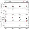 |
Fig. 3 Comparison between the velocity centroids, vc, and line widths, Δv, of the [CII] and CRRL line profiles. vc and Δv are determined from a multicomponent Gaussian fit to the observed spectra (Fig. 2). The top panel shows the velocity centroids, the upper middle panel shows the difference between the closest velocity centroids in units of its error, Z score, the lower middle panel shows the standard deviation of the Gaussian line profile, and the lower panel shows the ratio Δv([CII])∕Δv([CRRL]). The starred symbols show the [CII] components that are closest in velocity to the CRRLs. |
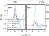 |
Fig. 4 Spectra of the [CII] and [13CII] F = 2– 1 lines toward EFF4 (left) and EFF5 (right). The [13CII] line has beenscaled by the 13C abundance ([12C/13C] = 67, Langer & Penzias 1990), and the relative strength of its hyperfine component (0.625, Ossenkopf et al. 2013). The scaled [13CII] line is brighter than the [CII] line, which suggests that the latter is optically thick, or that there is self-absorption. In the left panel we show the results of modeling the [CII] emission considering self-absorption of the background emission by a foreground component. In this figure, we averaged the [13 CII] line to a channel width of 0.8 km s−1. |
3.3 Comparison with molecular gas tracers
We compare the averaged CRRLs to the HCN(1–0) and C2 H(1–0) lines in the right panels of Fig. 2. There is good agreement between the line profiles, with offsets < 1 km s−1 in the velocity centroids of the lines. In terms of their widths, the CRRLs are slightly broader than the molecular lines, though their widths are consistent given the uncertainties. The overall agreement between the molecular lines and the CRRLs confirms that the CRRL emission is associated with the neutral gas in the ISF.
Toward EFF1 the HCN(1–0) and C2 H(1–0) lines are detected at a velocity of ≈ 12 km s−1, redshifted with respect to the [CII] line (≈ 10 km s−1, Fig. 2). The detection of the molecular lines shows that there is molecular gas along the line of sight, and the velocity shift with respect to the warmer neutral material indicates that these gases are not moving at the same speed. The nondetection of the CRRLs along the ≈ 2 km s−1 velocity shift between [CII] and HCN suggests that the gas in this region is being dispersed, and that the C+ layer is less dense than in other regions.
In Fig. 5 we compare the intensity of the averaged CRRLs and the HCN(1–0) line. There, we observe that their intensities are anticorrelated, HCN(1–0) is brighter toward EFF1 and its intensity decreases as we move to EFF5, while the CRRLs are not detected toward EFF1 and are brighter toward EFF5. Naively, we would assume that this anticorrelation can be explained by an increase in the C+ column density as we move from EFF1 to EFF5. We return to this anticorrelation in Sect. 4.1.2, once we have derived the properties of the C+ layer.
The similarity between the CRRL profile and those of other tracers of the neutral gas in the ISF (Fig. 2), confirms that the CRRL emission is associated with the neutral gas in the envelope of the ISF. During the rest of the analysis, we assume that the CRRLs trace the C+ layer in the envelope of the ISF.
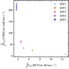 |
Fig. 5 Intensity of the averaged CRRLs as a function of the intensity of the HCN(1–0) line. The intensities of both lines are anticorrelated. The error bars are 1σ, and the inverted triangle shows the 3σ upper limit for the CRRL intensity toward EFF1. |
4 Analysis
In this section we derive the electron density, temperature, C+ column density and size along the line of sight of the C+ layer of the ISF using the averagedCRRLs, [CII] and [13CII] F = 2–1 lines. Then,we constrain the ionization fraction deeper into the ISF using the HCN(1–0) and C2 H(1–0) J = 1∕2–1∕2 lines.
4.1 C+ layer properties
In this subsection we focus on the properties of the C+ layer. We start by describing the model used to derive the properties of this layer, then we present the gas properties derived by comparing the observations to the model predictions, and we end by discussing the uncertainties of this modeling.
4.1.1 Model
We model the properties of the C+ layer of the PDR on the surface of a molecular cloud as a plane parallel homogenoeus slab of gas. We assume that throughout the slab carbon is singly ionized, and that it is the dominant donor of free electrons so x(C+) = x(e−) = 1.5 × 10⁻⁴ (Sofia et al. 2004). This is a good approximation in the C+ layer of a PDR (e.g., Salas et al. 2019). We also assume that the amount of molecular and atomic gas in the slab is the same, that is,  . Since we assume that the gas properties are homogeneous in the C+ layer, we have that the CRRL, [CII] and [13CII] F = 2–1 emission originates from the same volume of gas and that their emission fills the telescope beam.
The brightness temperature of the FIR C+ line is given by (e.g., Goldsmith et al. 2012)
![Mathematical equation: \begin{equation*}T_{\mathrm{B}}(\mbox{[CII]})\,{=}\,T^{*}\left(\frac{1}{e^{T^{*}/T^{\mathrm{ex}}}-1}-\frac{1}{e^{T^{*}/T^{\mathrm{bg}}}-1}\right)(1-e^{-\tau}),\end{equation*}](/articles/aa/full_html/2021/09/aa40670-21/aa40670-21-eq10.png) (1)
(1)
with
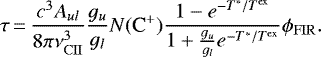 (2)
(2)
Here Aul = 2.36 × 10⁻⁶ s−1 is the spontaneous decay rate for the 158 μm-[CII] line (Wiese & Fuhr 2007), νCII is the frequency of the line (1900.5369 GHz for [CII] and1900.4661 GHz for [13CII] F = 2–1, Cooksy et al. 1986), gu and gl are the statistical weights of the upper (J = 3∕2) and lower (J = 1∕2) levels, T* = ΔE∕kB = 91.25 K is the energy difference between the upper and lower levels, Tex is the excitation temperature, Tbg is the temperature of the background continuum and ϕFIR the line profile in units of km s−1. Tex is determined from the solution to the detailed balance problem, considering collisions with electrons, atomic and molecular hydrogen, and the rates given in Goldsmith et al. (2012). We assume the same excitation temperature for the [CII] and [13 CII] lines. To predict the brightness temperature of the [13CII] F = 2–1 line we adopt a [12 C/13C] abundance ratio of 67 (Langer & Penzias 1990), and a relative strength of 0.625 (Ossenkopf et al. 2013).
For a transition from upper level n′ to n the brightness temperature of a CRRL is given by (e.g., Dupree 1974)
 (3)
(3)
with
 (4)
(4)
where bn and  are the departure coefficients, Tcont the brightness temperature of the background continuum, h Planck’s constant, e the electron charge, kB the Boltzmann constant,
  the mass of the electron, c the speed of light, χn = 157 800n−2T−1,
  the oscillator strength of the transition, T is the gas temperature,
  is the density of electrons,
  is the column density of ionized carbon, ϕCRRL the line profile in units of Hz−1 and l is the size of the C+ layer along the line of sight. To compute the departure coefficients we follow Salgado et al. (2017a), and compute them for
  between 0.01 and 200 cm−3 and T between 10 and 103 K. For the oscillator strength we use the approximation by Menzel (1968), valid for transitions of hydrogenic atoms at large n and small Δn = n′− n.
To determine the gas properties, we compare the averaged CRRLs, [CII] and [13 CII] F = 2–1 lines and their ratios to the model predictions. We require that the model matches the observations to within 3σ, and the FIR data are convolved to 126′′ to match the resolution of the radio lines. For the [CII] line we use the brightest velocity component that is consistent with the velocity centroid of the averaged CRRLs and [13CII] F = 2–1 lines.
In summary, our model takes as inputs the gas temperature, electron density and C+ column density, and from these inputs it predicts the intensities of the n = 106 CRRL, and the FIR lines of C+. These intensities are then compared to the observations (Tables 3, 4 and A.1) to determine the temperature,  and N(C+). From these values we also derive the size of the C+ layer along the line of sight, the thermal pressure, and the thermal and nonthermal line widths.
Gas and line properties derived from the analysis of the CRRLs and the FIR C+ lines.
Column densities.
4.1.2 Gas properties
The gas properties derived using our model are presented in Table 5. For EFF4 and EFF5 the gas properties are well constrained, while for EFF2 the lower S/N of the spectra results in larger uncertainties. For regions without a [13 CII] detection (EFF1 and EFF3), we do not derive gas properties. For EFF4 and EFF5,  cm−3 which corresponds to a gas density nH ~5 × 103 cm−3.
The thermal pressure for the gas is pth = (4.0 ± 0.5) × 105 K cm−3 and (2.3 ± 0.4) × 105 K cm−3 for EFF5 and EFF4, respectively. These thermal pressures are smaller than those in the PDRs of NGC 1977 ((4– 9) × 105 K cm−3, Pabst et al. 2020) and the Orion Bar ((2– 4) × 108 K cm−3, Cuadrado et al. 2019), both of which are exposed to a higher radiation field than the regions studied here.
The C+ column densities (Table 5) are converted to hydrogen column densities using N(H) = N(C+)∕x(C+) and are presented in Table 6. The derived N(H) is 20 and 80% of the dust derived column density for EFF4 and EFF5, respectively. The warmer region (EFF5) shows a higher fraction of the gas in the C+ layer. This might reflect the fact that EFF5 is exposed to a higher radiation field, hence has a larger C+ layer, or that for warmer regions the assumption of isothermal dust along the line of sight biases the dust derived column densities toward lower values.
Our model and the observations are consistent with optically thick [CII] lines (Table 5). For a [CII] optical depth τ([CII]) ≈ 10 the lines would appear to be a factor of two broader due to opacity broadening. This is consistent with the measured line widths (Fig. 3 bottom).
In Fig. 5 we observed an anticorrelation between the intensities of the CRRLs and the HCN(1–0) line. The derived C+ column densities (Table 5) increase from EFF2 to EFF5, which would explain the observed relation. As the C+ column density increases, so does the CRRL intensity, while the HCN column density and the HCN(1–0) intensity decrease. This implies that, in general, the detection of molecular gas and/or bright [CII] does not guarantee the detection of CRRLs. Given the present observations we detect the C102α and C109α CRRLs from regions with N(C+) ≳ 5 × 1016 cm−2. This means that C-band (4–8 GHz) observationsof CRRLs, where a total of 24 Cα RRLs can be observed, is limited to the study of regions with N(C+) ≳ 1 × 1016 cm−2 using current instruments. This is a loose lower limit, as colder and/or denser regions could be observed at lower column densities.
4.1.3 Uncertainties
The largest uncertainties in the derived gas properties arise from (i) the decomposition of the [CII] line profiles into Gaussian components, (ii) the prescence of foreground [CII] absorption and (iii) the assumption that [CII], [13 CII] and the CRRLs trace the same volume of gas. Here we explore how these effects affect the derived gas properties.
To test how (i), the decomposition of the [CII] line profiles into Gaussian components, affects our results we vary the [CII] intensity. We perform this analysis toward EFF4 and EFF5 as these are the regions with the highest S/N detections. For EFF5 we find that decreasing the intensity of the [CII] line by a factor of 0.8 increases the electron density to 1.4 ± 0.2 cm−3 and lowers the temperature to 50 ± 5 K, while the C+ column density remains almost the same, (4 ± 0.3) × 1018 cm−2. And, if we increase the [CII] intensity by a factor of 1.5 we have T = 60 ± 7 K,  cm−3 and N(C+) = (3.8 ± 0.4) × 1018 cm−2. For EFF4 if we increase the intensity of the [CII] line by 1.5 the derived temperature is 65 ± 11 K,
 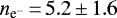 cm−3 and N(C+) = (1.6 ± 0.5) × 1018 cm−2. This shows that altough the derived gas properties are sensitive to the decomposition of the [CII] line profiles, the results remain consistent.
The effects of (ii), the presence of foreground [CII] absorption, would depress the background [CII] line profile. Toward EFF4 we could use the results of the [CII] line decomposition (Table A.1) when considering self-absorption. However, when we use this decomposition our model only provides a lower limit to the gas temperature and electron density because of the large uncertainties in the best fit line parameters. We place upper limits to the temperature of the gas in the C+ layer using the results from the PDR toolbox (Kaufman et al. 2006; Pound & Wolfire 2008). The PDR toolbox predicts the gas temperature at the surface of the PDR given G0 and the gas density. For G0, we use the values derived from the dust temperature, and for the density the lower limits to the electron density (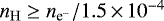 ). Toward EFF4 we have that the gas is exposed to a radiation field of G0 ≈ 35 and has a density > 103 cm−3, thus the surface temperature is expected to be ≤100 K. This sets an upper limit to the electron density of
  cm−3. Then, from the upper and lower limits, the electron density is constrained to 0.3 cm−3 ≤
 ≤ 10 cm−3 and the gas temperature to 30 K ≤ T ≤ 100 K. The lower limits are consistent with the electron density and temperature derived from the emission only analysis, but the upper limits on the density is a factor of 15 larger. We note that the upper limit is unlikely, since it would imply a gas thermal pressure of pth ≈ 7 × 10⁶ K cm−3, which is larger than the thermal presure in the PDR of NGC 1977 (Pabst et al. 2020), and would conflict with the nondetection of the C76α line toward EFF4 by Kutner et al. (1985). When considering self-absorption, the [CII] optical depth is 0.5 (1.6) and Tex ≈ 200 K (80 K) for the background (foreground) components, resulting in a similar column density N(C+) ~ 1018 cm−2. This analysis shows that when we consider the prescence of [CII] self-absorption, the gas temperature and density could be consistent or larger than the values presented in Table 5.
To test (iii), assuming that [CII], [13CII] and the CRRLs trace the same volume of gas, we compare the predictions of our model to independent observations. We compare to results of the C76α observations that Kutner et al. (1985) obtained with the NRAO 43 m telescope at 120′′ resolution. EFF4 and EFF5 show significant overlap with some of their observations (Fig. 1 right). Close to EFF5 they report a line peak of 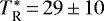 mK, a line width of Δv = 0.8 km s−1 and an intensity
 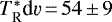 mK for the line at vc = 11.5 km s−1. Given the values and uncertainties they report, we find that the line intensity and its uncertainty are underestimated. Here we compute an intensity of
 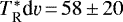 mK, given the line peak and width (adopting an error on the line width of 0 km s−1). Toward EFF5 we predict a C76α intensity of 95 ± 2 mK km s−1, consistent with the value we derived. Close to EFF4 they report a nondetection of the C76α line with a 3σ upper limit of
  mK, for which we predict
  mK. The agreement between our model predictions and the C76α observations suggests that modeling the FIR [CII] and [13CII] lines as arising from the same volume as the CRRLs is a reasonable assumption.
An additional test to our model comes from comparing the derived gas properties to those derived by Kutner et al. (1985). Kutner et al. (1985) derive a temperature of T ≈ 35 K and  cm−3 from the C110α and C76α line ratio at 396′′ resolution on the edge of the HII region NGC 1977, encompassing EFF5. They estimate a factor of two uncertainty in the gas properties, which could explain the difference in temperature, but not the factor of three difference in
  . The remaining difference in density can be explained by the different departure coefficients used (bn ≈ 0.05 using Walmsley & Watson (1982) and bn ≈ 0.07 using Salgado et al. (2017a) for ne = 10 cm−3 and T = 20 K) and the use of an approximation to compute the Cnα optical depth by Kutner et al. (1985) (they approximate the last term in parenthesis in Eq. (4), which is not a good approximation for n < 100). These differences would lead us to derive densities that are a factor of two lower than those of Kutner et al. (1985), bringing our results into agreement.
For a fixed temperature and size of the region along the line of sight the electron density is proportional to the square root of the brightness of the CRRLs. Thus, if the observed lines are beam diluted at 126′′ resolution then the derived electron densities are underestimated. Conversely, for a fixed line brightness  increases with temperature and decreases for larger column densities. If the CRRL and [CII] emission have a similar spatial extent (as suggested by the observations of Wyrowski et al. 1997 on 0.02 pc scales toward the Orion Bar), then beam dilution is not significant at 126′′.
Our observations sample the gas at 126′′ resolution (0.25 pc at the distance of Orion A). At this resolution we expect that multiple clumps and structures will be unresolved, hence the derived gas properties are an average of the properties of individual clumps and filaments within the beams. Additionally, since the line intensities of the CRRLs and the [CII] line have different dependencies on the gas temperature and density, they will trace different portions of the C+ layers within the telescope’s beam. If the temperature and density gradients are large in the C+ layer, then using an homogeneous model will result in biased gas properties. In particular, the gas temperatures and densities could be biased toward higher values. The comparison between the predictions of our model and the results of Kutner et al. (1985) suggests that in the regions studied these gradients are small enough that this effect does not significantly affect our results. Using a model that takes into account the temperature and density gradients can reduce these biases (e.g., Salas et al. 2019). Another consequence of the differences in how the radio and FIR C+ lines respond to temperature and density, is that on scales <0.02 pc we expect to start observing differences between their spatial distributions. If the differences between the spatial distributions of the CRRLs and the [CII] line are resolved, then the use of a homogeneous model for the C+ layer is also expected to produce biased results.
Lastly, we consider the influence of the choice of the molecular gas fraction, and the principal quantum number adopted for the averaged CRRLs. We estimate that the molecular gas fraction has a small effect on the derived gas proprieties. If we use  , the derived gas density and temperature are lower by 8 and 13%, respectively. Increasing the fraction of molecular gas to 90% has no noticeable effect on the derived gas properties. For the principal quantum number, if we used n = 109 for the averaged CRRLs, then the gas temperature increases by 10% and there is no noticeable change in the electron density.
4.2 Gas traced by HCN
Here we focus on the properties of the gas traced by HCN. First we assess whether the CRRLs and HCN(1–0) trace the same volume of gas, and then we proceed to derive the ionization fraction of the gas using molecular lines.
4.2.1 HCN & CRRLs
The comparison between the HCN(1–0) line and the CRRLs (Sect. 3.3) shows that both trace the ISF. However, from our data alone it is not clear whether both lines probe the same volumes of gas. Here, we use results from the literature and the gas properties derived for the C+ layer to answer this.
Wyrowski et al. (2000) observed NGC 2023 at higher spatial resolution (≈10′′) in CRRLs and HCN(1–0). Their observations show differences in the spatial distribution of both tracers, with CRRLs tracing gas closer to the exciting star than the HCN(1–0) line. Although the properties of NGC 2023 are different from those of the OMC-2/3, their results suggest that both lines do not trace the same volumes of gas.
Another comparison between CRRLs and HCN(1–0) comes from the gas temperature. Hacar et al. (2020) showed that the HCN/HNC intensity ratio, for the J = 1–0 lines, is an accurate probe of the gas temperature, and that the temperatures derived from this ratio are similar to the ones derived from the lines of ammonia (Friesen et al. 2017) and analysis of the FIR emission from dust (Lombardi et al. 2014). In Table 7 we present the gas temperature derived from the ammonia lines (Friesen et al. 2017), the HCN/HNC ratio (Hacar et al. 2020) and that derived for the C+ layer (Sect. 4.1). The temperatures derived from the ammonia lines and the HCN/HNC ratio are consistent, while the C+ layer is warmer. This confirms that in the OMC-2/3 the HCN(1–0) line probes a different volume of gas than the CRRLs.
Gas temperature.
4.2.2 Ionization fraction of the molecular gas
To constrain the ionization fraction of the gas traced by the HCN(1–0) line we use the analytical fits of Bron et al. (2021). These analytical fits provide x(e−) as a function of the ratios of the intensity or the column density of different tracers. The analytical fits are derived by varying the physical conditions (e.g., temperature, density, radiation field, AV, CRIR) usedas input for the chemical network of Roueff et al. (2015). This produces column densities for the species being considered which are then used to estimate line intensities using the non-LTE radiative transfer program RADEX (van der Tak et al. 2007). We use their results for dense cold clouds, as the visual extinction is > 7 toward the regions studied.
Here we use the intensity ratios of the C2 H(1–0) J = 1∕2–1∕2 F = 0–1 and HCN(1–0) lines. We use this ratio, as the lines have been observed simultaneously (Melnick et al. 2011), and variations in this intensity ratio can be explained by variations in x(e−) (Bron et al. 2021). One major caveat of using these lines is that they do not trace the same volume of gas. As shown by observations of the Orion Bar by van der Wiel et al. (2009), HCN and C2 H do not trace the same volumes of gas, with C2H tracing gas closer to the source of radiation (the Trapezium stars). Since the analytical expressions derived by Bron et al. (2021) are based on a one zone model (i.e., there is no spatial information), this implies that the ionization fractions derived from this ratio will be an average of the ionization fractions in the volumes probed by C2 H and HCN, and thus can only be usedas upper limits to x(e−) in the gas probed by the HCN(1–0) line.
The line ratios for EFF1, EFF4 and EFF5 are presented in Fig. 6. The ratios are consistent with being constant along the RA direction and have values ≈0.06, which corresponds to x(e−) ≲ 3 × 10⁻⁶ in the gas probed by HCN. This upper limit to the ionization fraction is a factor of a few larger than the typical values found toward dense cores x(e−) ~ 10−8–10−6 (e.g., Caselli et al. 1998; Bergin et al. 1999).
Away from the spine of the ISF the C2 H(1–0) J = 1∕2–1∕2 F = 0–1 line is not detected. In these regions we use the C2 H(1–0) J = 1∕2–1∕2 F = 1–1 line to estimate the ionization fraction by assuming a ratio of 2 between the F = 1–1 and F = 0–1 lines. The ratio shows small variations along the slices and is consistent with the ionization fraction observed toward the center of the ISF (Fig. 6 bottom). These results show that the average ionization fraction remains relatively high (x(e−) ≈ 3 × 10⁻⁶) in the lowercolumn density regions away from the spine of the ISF. If we use the analytical expressions for translucent clouds then the derived ionization fractions would be a factor of 2.5 larger.
Additional information on the ionization fraction of the molecular gas can be obtained from observations of deuterated molecules. Assuming steady-state chemistry it can be shown that RD ≡[DCO+]/[HCO+] (e.g., Caselli et al. 1998; Caselli 2002). Around EFF5, Kutner et al. (1985) reports a DCO+/H13CO+ intensity ratio of ≈0.5 (their Fig. 10). For comparison, Bergin et al. (1999) finds DCO+/H13CO+ intensity ratios ≈(1.3–3.8) toward massive cores in Orion A and Orion B, which they use to derive an average ionization fraction x(e−) = (7.7 ± 0.1) × 10−8 for their sample of massive cores. Then, the results of Kutner et al. (1985) suggest that toward EFF5 the ionization fraction is higher than in the massive cores observed by Bergin et al. (1999). In either case, the properties of the molecular gas in EFF5 are reminiscent of those of a PDR rather than a massive core, and this higher level of ionization may reflect the photo-ionization of trace atoms with low ionization potentials such as S, Mg and Fe by penetrating UV photons.
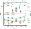 |
Fig. 6 Ratio between C2H(1–0) J = 1∕2–1∕2 and HCN(1–0) for EFF1, EFF4 and EFF5. We use this ratio to put an upper limit to x(e−) in the gas traced by HCN using the models of Bron et al. (2021) (right axis). Top: ratio between C2 H(1–0) J = 1∕2–1∕2 F = 0–1 and HCN(1–0) for EFF1, EFF4 and EFF5. Bottom: ratio between C2H(1–0) J = 1∕2–1∕2 F = 1–1 and HCN(1–0) for EFF1, EFF4 and EFF5. The intensity of the F = 1–1 line is scaled to that of the F = 0–1 line by assuming a 2:1 ratio. The ratios are computed by averaging over a slice of 2′ in the Dec direction centered in the regions. The offsets are shown along the RA direction and are referenced to the center of the region (Table 2). Inverted triangles show 3σ upper limits. |
5 Discussion
5.1 Velocity structure
High spatial (≈4′′) and spectral resolution observations of the ISF using optically thin tracers show the presence of multiple velocity components (e.g., Hacar et al. 2018; Zhang et al. 2020). These velocity components reflect a superposition of gas at different velocities along the line of sight, and are associated with the substructures, or fibers, that make up the ISF. At the spatial resolution of our CRRL observations these velocity components are likely to be blended (Hacar et al. 2018), which means that the measured line widths are likely overestimated.
Due to its high collisional excitation rates the FIR [CII] line probes a variety of physical conditions (neutral and ionized gas). The decomposition of the [CII] line profiles shows that 60–70% of the [CII] intensity is associated with the gas traced by CRRLs in the C+/C interface. The remaining velocity components in the [CII] line could be associated with photoevaporating gas from the surface of the molecular cloud. This gas would be warmer and less dense than the components associated with 5 GHz CRRL emission, resulting in the lack of CRRL detections from these velocity components.
5.2 Turbulence
The line widths contain information about the turbulence of the gas. Once the gas temperature is known, the nonthermal contribution to the line widths can be estimated from  , with
  and m the mass of the atom/molecule.
Toward EFF4 and EFF5, the line widths are dominated by nonthermal broadening (Table 5). The sound speed,  , of the neutral gas (μ = 1.6) is 0.48 ± 0.03 km s−1 and 0.53 ± 0.01 km s−1 toward EFF4 and EFF5, respectively. From this we have a sonic Mach number
  (EFF4) and 1.5 ± 0.1 (EFF5). We compare this to the sonic Mach number inferred from the ammonia lines (Friesen et al. 2017). Toward EFF4 they report σv = 0.44 ± 0.02 km s−1 and Tk = 21 ± 1 K. This implies that σv,th = 0.101 ± 0.003 km s−1, σv,nth = 0.43 ± 0.02 km s−1, and cs = 0.275 ± 0.007 km s−1 (μ = 2.33), so
  . And, toward EFF5 they find σv = 0.35 ± 0.03 km s−1 and Tk = 29 ± 2 K, for the component at 11.18 ± 0.03 km s−1. For the same component this implies, σv,th = 0.120 ± 0.005 km s−1, σv,nth = 0.32 ± 0.03 km s−1, and cs = 0.32 ± 0.01 km s−1, so
  . The sonic Mach numbers inferred for the C+ layer are in rough agreement with those derived from the ammonia lines. Magnetohydrodynamic (MHD) simulations of the ISM suggest that the sonic Mach number scales with density as
  up to densities of n ≈ 30 cm−3 and then flattens (e.g., Kritsuk & Norman 2004; Kritsuk et al. 2017). Our results are consistent with the scaling derived from MHD simulations, however, our observations likely do not properly resolve the velocity structure of the gas and might result in broader line profiles due to line blending (Sect. 5.1). CRRL observations with a higher spatial resolution could probe how turbulence changes from the envelope of the molecular cloud to its core.
From the nonthermal line widths we estimate the nonthermal pressure, 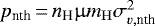 . Toward EFF4 and EFF5 the nonthermal pressures are (1.3 ± 0.5) × 106 K cm−3 and (8 ± 1) × 105 K cm−3, respectively. The nonthermal pressure is larger than the thermal pressure of the gas, pth = (1.9 ± 0.4) × 105 K cm−3 and (3.5 ± 0.1) × 105 K cm−3 for EFF4 and EFF5, respectively. This suggests that the gas is supported by turbulence.
5.3 Excitation of HCN
Here we explore the importance of collisional excitation by electrons, cosmic ray heating and radiative trapping on the intensity of the HCN(1–0) line. To estimate how the HCN(1–0) intensity changes when considering collisions with electrons we use RADEX (van der Tak et al. 2007) and the collisional rate coefficients calculated by Faure et al. (2007) and Dumouchel et al. (2010) for collisions with H2 and e−, respectively.To estimate the effect of cosmic-ray heating we derive the CRIR using simplified analytical results and then determine the gas equilibrium temperature by balancing the gas heating and cooling rates through the use of the Derive the Energetics and SPectra of Optically Thick Interstellar Clouds code (DESPOTIC, Krumholz 2014). DESPOTIC includes approximations for the dominant gas heating and cooling mechanisms and uses a one-zone model to determine the gas equilibrium temperature. To compute theline cooling it uses the escape probability formalism. We assess the effect of radiative trapping by estimating the HCN(1–0) optical depth from its fine structure components.
To investigate the HCN intensity using RADEX we adopt a gas temperature of 23 K, consistent with the temperature of the molecular gas toward EFF4 and EFF5 (Table 7), and assume a plane parallel geometry. From the derived path lengths (Table 5) and the total column densities (Table 6) we estimate gas densities of (1.9 ± 0.5) × 104 cm−3 (EFF4) and (7 ± 2) × 103 cm−3 (EFF5). Adopting our upper limit to x(e−), these densities correspond to  cm−3 (EFF4) and 0.021 cm−3 (EFF5). For these conditions, we compute the HCN(1–0) intensity with and without electrons as collisional partners. Including collisions with electrons produces a 12% increase in the HCN(1–0) intensity in both cases, almost independent of the adopted HCN column density. The effect is more pronounced at lower temperatures, for example, at 10 K the increase is 20%.
As discussed in Sect. 4.2, the properties of the molecular gas toward EFF5 seem to be closer to those of the gas in a PDR than the gas in a molecular core. Past the C+ layer of a PDR, the ionization fraction of the gas is set by the photo-ionization of trace atoms, and, past the PDR boundary, in the molecular core by cosmic-ray ionization. It is only at an AV ~ 10, that the ionization of trace atoms (particularly of sulfur and magnesium) can result in x(e−) ~ 10−6, consistent with our upper limits for the HCN traced gas. If the HCN gas is probing regions at an AV ~ 10 then, we do expect that cosmic-ray heating will be the dominant heating mechanism, as the attenuation of the FUV field this deep in the PDR results in a weak contribution from photoelectric heating.
The equilibrium temperature of the gas is set by the balance between heating and cooling. For the gas in the C+ layer the dominant heating mechanism is photoelectric heating, and the cooling is mainly through the [CII] line. Deeper into the cloud (AV > 7), the heating is mainly due to cosmic ray heating, and cooling is dominated by CO emission. The gas heating and cooling rates will depend on the gas density, the CRIR, and the abundances of the dominant cooling elements. Thus, to estimate the equilibrium temperature, and the effect of cosmic-ray heating, we need to estimate the CRIR.
If cosmic-ray ionization is the dominant ionization mechanism, then the ionization fraction is set by the balance between cosmic-ray ionization and recombination, so 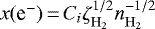 . Based on an analytical model, McKee (1989) derive Ci = 3.2 × 103 cm−3∕2 s1∕2. For a gas density of 1.6 × 104 cm−3 and an ionization fraction ≤3 × 10⁻⁶ this corresponds to
  s−1. We also estimate the CRIR from the RH ≡ x(HCO+)∕x(CO) ratio. Ohashi et al. (2014) observed H13 CO+ toward the millimeter bright source MMS 2 (or TUKH003 in Tatematsu et al. 1993), a dense core that contains a MIR binary system (Nielbock et al. 2003) within the EFF4 area, and find N(H13CO+) = 4.1 × 1012 cm−2 over a 31.′′5 beam. Toward the same source
 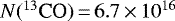 cm−2 (Berné et al. 2014), so RH ≡ [HCO+]/[CO] = 6 × 10⁻⁵. Using Eq. (2) of Caselli et al. (1998) we find ζ ≤ 3 × 10⁻¹⁵ s−1 for a temperature of 30 K. Both upper limits on the CRIR are consistent with the nondetection of HRRLs associated with the cold neutral gas toward EFF4, which implies ζp ≤ 8 × 10¹⁴ s−1 (Neufeld & Wolfire 2017). A more precise determination of the CRIR would require a measurement of the ionization fraction for the molecular gas.
We use the upper limits to the CRIR to estimate the gas equilibrium temperature. To model the gas probed by HCN we adopt a density of 1.6 × 104 cm−3, a column density of 6.5 × 1022 cm−2, a CRIR of 3 × 10⁻¹⁵ s−1 and the parameters for a giant molecular cloud in the Milky Way (Krumholz 2014). We find an equilibrium temperature of ~ 45 K, which is larger than the temperature of the molecular gas inferred from the HCN/HNC ratio and NH3 lines (Table 7). This suggests that the CRIR is well below our upper limit. If we adopt a standard CRIR of 2.5 × 10⁻¹⁷ s−1, then the equilibrium temperature is ~8 K. To match the temperatureof the molecular gas, 23 K, the CRIR should be 5 × 10⁻¹⁶ s−1, comparable to the values inferred toward dense cores (e.g., Caselli et al. 1998). An increase in the gas temperature from 8 to 23 K results in a factor of 2.6 increase in the HCN(1–0) intensity.
Radiative trapping becomes important when the gas is optically thick. Melnick et al. (2011) estimate that the HCN(1–0) optical depth is ≤1.5, and less than unity for 90% of the regions where the hyperfine components are detected. An optical depth of 1.5 results in an escape probability of 0.2 for a plane parallel slab, which lowers the critical density of the transition by the same amount (e.g., Shirley 2015). Since the highest optical depths are measured toward the high column density regions, radiative trapping does not explain the extended HCN emission.
These results suggest that toward the spine of the ISF, the HCN(1–0) emission is caused by the presence of warm HCN. This is similar to the findings of Barnes et al. (2020), who find that the HCN(1–0) intensity per unit column density is higher in the warmer regions around W49. Our analysis suggest that in these regions the gas temperature is set by cosmic-ray heating with a CRIR ~ 5 × 10⁻¹⁶ s−1.
6 Summary
We present observations of the C102α and C109α lines toward five positions along the OMC-2 and OMC-3, with detections in four of these positions. We average these CRRLs to increase the S/N of the spectra during our analysis. Below, we summarize our findings.
The optically thin CRRLs are detected at velocities of vLSR ≈ 10–12 km s−1, consistent with the velocity of the ISF in other tracers, such as 158 μm-[CII], CO, HCN, and C2H. The width of the line is Δv ≈ 2 km s−1 which confirms that the line traces cold gas (T < 100 K) in the C+/C interfaceof the ISF.
We compare the intensities of the CRRLs, [13CII] F = 2–1 and [CII]lines to the predictions of a homogeneous model of the C+/C interface. For the velocity components detected in the three lines with a SNR ≥ 5 we find electron densities of
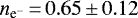 cm−3 (EFF4) and 0.95 ± 0.02 cm−3 (EFF5), and gas temperatures of T = 45 ± 5 K (EFF4) and 55 ± 2 K (EFF5). These electron densities correspond to a gas density of ~5 × 103 cm−3, and, combined with the gas temperature, a gas thermal pressure pth ≈ 4 × 10⁵ K cm−3.
For thesesame regions the temperature of the molecular gas is ≈25 K, based on the HCN/HNC ratio and the NH3 lines. The difference in the temperatures derived from the C+ lines and the molecular lines leads us to conclude that they do not trace the same volumes of gas.
We use the C2H(1–0) J = 1∕2–1∕2 and HCN(1–0) lines to constrain the ionization fraction in the denser regions of the molecular cloud using the models of Bron et al. (2021). We find x(e−) ≤ 3 × 10⁻⁶.
We use the ionization fraction of the molecular gas to estimate how collisional excitation with electrons influences the HCN emission. We find that collisions with electrons contribute ≤12% to the line intensity.
Future observations of CRRLs and HCN in low column density regions will provide further insight into the excitation of HCN in the extended envelopes of molecular clouds.
Acknowledgements
The authors thank Gary Melnick and Volker Tolls for sharing their HCN and C2 H data cubes. M.R.R. would like to thank B. Winkel, C. Kasemann, A. Kraus and the telescope staff for their support with the setup, conduction and reduction of the observations with the Effelsberg 100m radio telescope, as well as A. Jacob and Y. Gong for useful discussions on the removal of baseline ripples in the spectra observed with Effelsberg. This work was based on observations with the 100-m telescope of the MPIfR (Max-Planck-Institut für Radioastronomie) at Effelsberg. This research made use of Astropy, a community-developed core Python package for Astronomy (Astropy Collaboration 2013, 2018), matplotlib, a Python library for publication quality graphics (Hunter 2007), LMFIT, a nonlinear least-square minimization and curve-Fitting package for Python (Newville et al. 2014), and CRRLpy, a Python package for the analysis of RRL observations (Salas et al. 2016).
Appendix A Best fit Gaussian components
Here we provide the best fit line properties for the [CII] line.
Best fit [CII] line properties.
References
- Akaike, H. 1974, IEEE Transac. Automat. Control, 19, 716 [Google Scholar]
- Astropy Collaboration (Robitaille, T. P., et al.) 2013, A&A, 558, A33 [NASA ADS] [CrossRef] [EDP Sciences] [Google Scholar]
- Astropy Collaboration (Price-Whelan, A. M., et al.) 2018, AJ, 156, 123 [Google Scholar]
- Bally, J., Langer, W. D., Stark, A. A., & Wilson, R. W. 1987, ApJ, 312, L45 [NASA ADS] [CrossRef] [Google Scholar]
- Barnes, A. T., Kauffmann, J., Bigiel, F., et al. 2020, MNRAS, 497, 1972 [CrossRef] [Google Scholar]
- Bergin, E. A., Plume, R., Williams, J. P., & Myers, P. C. 1999, ApJ, 512, 724 [NASA ADS] [CrossRef] [Google Scholar]
- Berné, O., Marcelino, N., & Cernicharo, J. 2014, ApJ, 795, 13 [NASA ADS] [CrossRef] [Google Scholar]
- Black, J. H., & van Dishoeck, E. F. 1991, ApJ, 369, L9 [NASA ADS] [CrossRef] [Google Scholar]
- Bron, E., Roueff, E., Gerin, M., et al. 2021, A&A, 645, A28 [NASA ADS] [CrossRef] [EDP Sciences] [Google Scholar]
- Burnham, K. P., & Anderson, D. R. 2004, Sociol. Methods Res., 33, 261 [Google Scholar]
- Caselli, P. 2002, Planet. Space Sci., 50, 1133 [NASA ADS] [CrossRef] [Google Scholar]
- Caselli, P., Walmsley, C. M., Terzieva, R., & Herbst, E. 1998, ApJ, 499, 234 [Google Scholar]
- Cooksy, A. L., Blake, G. A., & Saykally, R. J. 1986, ApJ, 305, L89 [NASA ADS] [CrossRef] [Google Scholar]
- Cuadrado, S., Salas, P., Goicoechea, J. R., et al. 2019, A&A, 625, L3 [CrossRef] [EDP Sciences] [Google Scholar]
- Dickinson, A. S., Phillips, T. G., Goldsmith, P. F., Percival, I. C., & Richards, D. 1977, A&A, 54, 645 [NASA ADS] [Google Scholar]
- Dumouchel, F., Faure, A., & Lique, F. 2010, MNRAS, 406, 2488 [NASA ADS] [CrossRef] [Google Scholar]
- Dupree, A. K. 1974, ApJ, 187, 25 [NASA ADS] [CrossRef] [Google Scholar]
- Dutrey, A., Duvert, G., Castets, A., et al. 1993, A&A, 270, 468 [Google Scholar]
- Evans, N. J., I. 1999, ARA&A, 37, 311 [NASA ADS] [CrossRef] [Google Scholar]
- Faure, A., Varambhia, H. N., Stoecklin, T., & Tennyson, J. 2007, MNRAS, 382, 840 [Google Scholar]
- Friesen, R. K., Pineda, J. E., co-PIs, et al. 2017, ApJ, 843, 63 [NASA ADS] [CrossRef] [Google Scholar]
- Gao, Y., & Solomon, P. M. 2004, ApJ, 606, 271 [NASA ADS] [CrossRef] [Google Scholar]
- Gatley, I., Becklin, E. E., Mattews, K., et al. 1974, ApJ, 191, L121 [Google Scholar]
- Ginsburg, A., & Mirocha, J. 2011, PySpecKit: Python Spectroscopic Toolkit [Google Scholar]
- Goicoechea, J. R., Pety, J., Gerin, M., Hily-Blant, P., & Le Bourlot, J. 2009, A&A, 498, 771 [NASA ADS] [CrossRef] [EDP Sciences] [Google Scholar]
- Goicoechea, J. R., Teyssier, D., Etxaluze, M., et al. 2015, ApJ, 812, 75 [NASA ADS] [CrossRef] [Google Scholar]
- Goldsmith, P. F., & Kauffmann, J. 2017, ApJ, 841, 25 [Google Scholar]
- Goldsmith, P. F., Langer, W. D., Pineda, J. L., & Velusamy, T. 2012, ApJS, 203, 13 [Google Scholar]
- Gordon, M. A., & Sorochenko, R. L., eds. 2009, Astrophys. Space Sci. Lib., 282 [CrossRef] [Google Scholar]
- Guevara, C., Stutzki, J., Ossenkopf-Okada, V., et al. 2020, A&A, 636, A16 [CrossRef] [EDP Sciences] [Google Scholar]
- Habing, H. J. 1968, Bull. Astron. Inst. Netherlands, 19, 421 [Google Scholar]
- Hacar, A., Tafalla, M., Forbrich, J., et al. 2018, A&A, 610, A77 [NASA ADS] [CrossRef] [EDP Sciences] [Google Scholar]
- Hacar, A., Bosman, A. D., & van Dishoeck, E. F. 2020, A&A, 635, A4 [CrossRef] [EDP Sciences] [Google Scholar]
- Herbst, E., & Klemperer, W. 1973, ApJ, 185, 505 [NASA ADS] [CrossRef] [Google Scholar]
- Heyminck, S., Graf, U. U., Güsten, R., et al. 2012, A&A, 542, L1 [NASA ADS] [CrossRef] [EDP Sciences] [Google Scholar]
- Hoang-Binh, D., & Walmsley, C. M. 1974, A&A, 35, 49 [Google Scholar]
- Hollenbach, D. J., & Tielens, A. G. G. M. 1999, Rev. Mod. Phys., 71, 173 [Google Scholar]
- Hollenbach, D. J., Takahashi, T., & Tielens, A. G. G. M. 1991, ApJ, 377, 192 [NASA ADS] [CrossRef] [Google Scholar]
- Hunter, J. D. 2007, Comput. Sci. Eng., 9, 90 [NASA ADS] [CrossRef] [Google Scholar]
- Kaufman, M. J., Wolfire, M. G., & Hollenbach, D. J. 2006, ApJ, 644, 283 [Google Scholar]
- Kauffmann, J., Goldsmith, P. F., Melnick, G., et al. 2017, A&A, 605, L5 [NASA ADS] [CrossRef] [EDP Sciences] [Google Scholar]
- Klein, B., Hochgürtel, S., Krämer, I., et al. 2012, A&A, 542, L3 [NASA ADS] [CrossRef] [EDP Sciences] [Google Scholar]
- Kraus, A. 2009, Calibration of the Effelsberg 100m telescope, Technical report, Max-Planck-Institut für Radioastronomie [Google Scholar]
- Kritsuk, A. G., & Norman, M. L. 2004, ApJ, 601, L55 [NASA ADS] [CrossRef] [Google Scholar]
- Kritsuk, A. G., Ustyugov, S. D., & Norman, M. L. 2017, New J. Phys., 19, 065003 [CrossRef] [Google Scholar]
- Krumholz, M. R. 2014, MNRAS, 437, 1662 [NASA ADS] [CrossRef] [Google Scholar]
- Kutner, M. L., Machnik, D. E., Mead, K. N., & Evans, N. J., I. 1985, ApJ, 299, 351 [NASA ADS] [CrossRef] [Google Scholar]
- Langer, W. D., & Penzias, A. A. 1990, ApJ, 357, 477 [Google Scholar]
- Lenz, D. D., & Ayres, T. R. 1992, PASP, 104, 1104 [NASA ADS] [CrossRef] [Google Scholar]
- Lombardi, M., Bouy, H., Alves, J., & Lada, C. J. 2014, A&A, 566, A45 [NASA ADS] [CrossRef] [EDP Sciences] [Google Scholar]
- Luisi, M., Anderson, L. D., Liu, B., Anish Roshi, D., & Churchwell, E. 2019, ApJS, 241, 2 [Google Scholar]
- McKee, C. F. 1989, ApJ, 345, 782 [NASA ADS] [CrossRef] [Google Scholar]
- McKee, C. F.,& Ostriker, E. C. 2007, ARA&A, 45, 565 [Google Scholar]
- Megeath, S. T., Gutermuth, R., Muzerolle, J., et al. 2012, AJ, 144, 192 [NASA ADS] [CrossRef] [Google Scholar]
- Meijerink, R., Spaans, M., Loenen, A. F., & van der Werf, P. P. 2011, A&A, 525, A119 [NASA ADS] [CrossRef] [EDP Sciences] [Google Scholar]
- Melnick, G. J., Tolls, V., Snell, R. L., et al. 2011, ApJ, 727, 13 [NASA ADS] [CrossRef] [Google Scholar]
- Menten, K. M., Reid, M. J., Forbrich, J., & Brunthaler, A. 2007, A&A, 474, 515 [NASA ADS] [CrossRef] [EDP Sciences] [Google Scholar]
- Menzel, D. H. 1968, Nature, 218, 756 [NASA ADS] [CrossRef] [Google Scholar]
- Mestel, L., & Spitzer, L., J. 1956, MNRAS, 116, 503 [NASA ADS] [CrossRef] [Google Scholar]
- Morris, M., Zuckerman, B., Turner, B. E., & Palmer, P. 1974, ApJ, 192, L27 [NASA ADS] [CrossRef] [Google Scholar]
- Natta, A., Walmsley, C. M., & Tielens, A. G. G. M. 1994, ApJ, 428, 209 [Google Scholar]
- Neufeld, D. A., & Wolfire, M. G. 2017, ApJ, 845, 163 [Google Scholar]
- Newville, M., Stensitzki, T., Allen, D. B., & Ingargiola, A. 2014, LMFIT: Non-Linear Least-Square Minimization and Curve-Fitting for Python [Google Scholar]
- Nielbock, M., Chini, R., & Müller, S. A. H. 2003, A&A, 408, 245 [NASA ADS] [CrossRef] [EDP Sciences] [Google Scholar]
- Ohashi, S., Tatematsu, K., Choi, M., et al. 2014, PASJ, 66, 119 [NASA ADS] [CrossRef] [Google Scholar]
- Oppenheimer, M., & Dalgarno, A. 1974, ApJ, 192, 29 [NASA ADS] [CrossRef] [Google Scholar]
- Ossenkopf, V., Röllig, M., Neufeld, D. A., et al. 2013, A&A, 550, A57 [NASA ADS] [CrossRef] [EDP Sciences] [Google Scholar]
- Ott, M., Witzel, A., Quirrenbach, A., et al. 1994, A&A, 284, 331 [NASA ADS] [Google Scholar]
- Pabst, C., Higgins, R., Goicoechea, J. R., et al. 2019, Nature [Google Scholar]
- Pabst, C. H. M., Goicoechea, J. R., Teyssier, D., et al. 2020, A&A, 639, A2 [CrossRef] [EDP Sciences] [Google Scholar]
- Pety, J., Guzmán, V. V., Orkisz, J. H., et al. 2017, A&A, 599, A98 [NASA ADS] [CrossRef] [EDP Sciences] [Google Scholar]
- Pound, M. W., & Wolfire, M. G. 2008, ASP Conf. Ser., 394, 654 [Google Scholar]
- Reid, M. J., Menten, K. M., Zheng, X. W., et al. 2009, ApJ, 700, 137 [NASA ADS] [CrossRef] [Google Scholar]
- Reipurth, B., Rodríguez, L. F., & Chini, R. 1999, AJ, 118, 983 [NASA ADS] [CrossRef] [Google Scholar]
- Risacher, C., Güsten, R., Stutzki, J., et al. 2016, A&A, 595, A34 [NASA ADS] [CrossRef] [EDP Sciences] [Google Scholar]
- Roueff, E., Loison, J. C., & Hickson, K. M. 2015, A&A, 576, A99 [NASA ADS] [CrossRef] [EDP Sciences] [Google Scholar]
- Roy, A. L., Teuber, U., & Keller, R. 2004, in European VLBI Network on New Developments in VLBI Science and Technology, 265 [Google Scholar]
- Salas, P., Morabito, L., Salgado, F., Oonk, R., & Tielens, A. 2016, CRRLpy: First pre-release [Google Scholar]
- Salas, P., Oonk, J. B. R., Emig, K. L., et al. 2019, A&A, 626, A70 [CrossRef] [EDP Sciences] [Google Scholar]
- Salgado, F., Morabito, L. K., Oonk, J. B. R., et al. 2017a, ApJ, 837, 141 [NASA ADS] [CrossRef] [Google Scholar]
- Salgado, F., Morabito, L. K., Oonk, J. B. R., et al. 2017b, ApJ, 837, 142 [Google Scholar]
- Shirley, Y. L. 2015, PASP, 127, 299 [Google Scholar]
- Siddiqui, S. A., Khan, S., & Qaiyum, A. 2020, MNRAS, 492, 1049 [NASA ADS] [CrossRef] [Google Scholar]
- Sofia, U. J., Lauroesch, J. T., Meyer, D. M., & Cartledge, S. I. B. 2004, ApJ, 605, 272 [NASA ADS] [CrossRef] [Google Scholar]
- Sorochenko, R. L., & Tsivilev, A. P. 2010, Kinemat. Phys. Celest. Bodies, 26, 162 [NASA ADS] [CrossRef] [Google Scholar]
- Tatematsu, K., Umemoto, T., Kameya, O., et al. 1993, ApJ, 404, 643 [NASA ADS] [CrossRef] [Google Scholar]
- Tielens, A. G. G. M. 2005, The Physics and Chemistry of the Interstellar Medium (Cambridge: Cambridge University Press) [CrossRef] [Google Scholar]
- Tsivilev, A. P. 2014, Astron. Lett., 40, 615 [CrossRef] [Google Scholar]
- van der Tak, F. F. S., & van Dishoeck, E. F. 2000, A&A, 358, L79 [NASA ADS] [Google Scholar]
- van der Tak, F. F. S., Black, J. H., Schöier, F. L., Jansen, D. J., & van Dishoeck, E. F. 2007, A&A, 468, 627 [NASA ADS] [CrossRef] [EDP Sciences] [Google Scholar]
- van der Wiel, M. H. D., van der Tak, F. F. S., Ossenkopf, V., et al. 2009, A&A, 498, 161 [NASA ADS] [CrossRef] [EDP Sciences] [Google Scholar]
- Vollmer, B., Gratier, P., Braine, J., & Bot, C. 2017, A&A, 602, A51 [NASA ADS] [CrossRef] [EDP Sciences] [Google Scholar]
- Walmsley, C. M., & Watson, W. D. 1982, ApJ, 260, 317 [NASA ADS] [CrossRef] [Google Scholar]
- Watson, W. D. 1972, ApJ, 176, 103 [NASA ADS] [CrossRef] [Google Scholar]
- Wiese, W. L., & Fuhr, J. R. 2007, J. Phys. Chem. Ref. Data, 36, 1287 [CrossRef] [Google Scholar]
- Winkel, B., Kraus, A., & Bach, U. 2012, A&A, 540, A140 [NASA ADS] [CrossRef] [EDP Sciences] [Google Scholar]
- Wyrowski, F., Schilke, P., Hofner, P., & Walmsley, C. M. 1997, ApJ, 487, L171 [NASA ADS] [CrossRef] [Google Scholar]
- Wyrowski, F., Walmsley, C. M., Goss, W. M., & Tielens, A. G. G. M. 2000, ApJ, 543, 245 [NASA ADS] [CrossRef] [Google Scholar]
- Young, E. T., Becklin, E. E., Marcum, P. M., et al. 2012, ApJ, 749, L17 [NASA ADS] [CrossRef] [Google Scholar]
- Zari, E., Brown, A. G. A., de Bruijne, J., Manara, C. F., & de Zeeuw, P. T. 2017, A&A, 608, A148 [NASA ADS] [CrossRef] [EDP Sciences] [Google Scholar]
- Zhang, C., Ren, Z., Wu, J., et al. 2020, MNRAS, 497, 793 [NASA ADS] [CrossRef] [Google Scholar]
Transitions involving a change in principal quantum number Δn = 1.
All Tables
Spectral setup of the C-band observations with the Effelsberg 100 m radio telescope.
Gas and line properties derived from the analysis of the CRRLs and the FIR C+ lines.
All Figures
|
Fig. 1 Location of the Effelsberg 5 GHz RRL observations presented in this work. Left: map of the peak temperature of the [CII] line over a one square degree centered on the Trapezium stars (Pabst et al. 2019). A green rectangle shows the extent of the region displayed on the right. Right: Spitzer IRAC 8 μm image of the OMC-2/3. The regions observed in 5 GHz RRLs are marked with solid black circles 1.′89 in diameter, while the dashed gray circles show the C76α observationsof Kutner et al. (1985) at 2′ resolution. The small green circles show the location of the sources detected in 3.6 cm radio continuum (Reipurth et al. 1999). |
| In the text | |
|
Fig. 2 CRRL spectra observed toward the northern part of the ISF with the Effelsberg 100 m radio telescope. The CRRL is an average of the C109α and C102α lines. We compare the averaged CRRL to the averaged HRRL (an average of the H109α and H102α lines, on the left), the FIR [CII] and [13CII] F = 2– 1 lines (center), and HCN(1–0) and C2 H(1–0) (right). In the center panels the [13CII] F = 2– 1 line is scaledto match the peak of the averaged CRRL, while on the right panels the CRRL is scaled to match the peak of the HCN(1–0) line. |
| In the text | |
|
Fig. 3 Comparison between the velocity centroids, vc, and line widths, Δv, of the [CII] and CRRL line profiles. vc and Δv are determined from a multicomponent Gaussian fit to the observed spectra (Fig. 2). The top panel shows the velocity centroids, the upper middle panel shows the difference between the closest velocity centroids in units of its error, Z score, the lower middle panel shows the standard deviation of the Gaussian line profile, and the lower panel shows the ratio Δv([CII])∕Δv([CRRL]). The starred symbols show the [CII] components that are closest in velocity to the CRRLs. |
| In the text | |
|
Fig. 4 Spectra of the [CII] and [13CII] F = 2– 1 lines toward EFF4 (left) and EFF5 (right). The [13CII] line has beenscaled by the 13C abundance ([12C/13C] = 67, Langer & Penzias 1990), and the relative strength of its hyperfine component (0.625, Ossenkopf et al. 2013). The scaled [13CII] line is brighter than the [CII] line, which suggests that the latter is optically thick, or that there is self-absorption. In the left panel we show the results of modeling the [CII] emission considering self-absorption of the background emission by a foreground component. In this figure, we averaged the [13 CII] line to a channel width of 0.8 km s−1. |
| In the text | |
|
Fig. 5 Intensity of the averaged CRRLs as a function of the intensity of the HCN(1–0) line. The intensities of both lines are anticorrelated. The error bars are 1σ, and the inverted triangle shows the 3σ upper limit for the CRRL intensity toward EFF1. |
| In the text | |
|
Fig. 6 Ratio between C2H(1–0) J = 1∕2–1∕2 and HCN(1–0) for EFF1, EFF4 and EFF5. We use this ratio to put an upper limit to x(e−) in the gas traced by HCN using the models of Bron et al. (2021) (right axis). Top: ratio between C2 H(1–0) J = 1∕2–1∕2 F = 0–1 and HCN(1–0) for EFF1, EFF4 and EFF5. Bottom: ratio between C2H(1–0) J = 1∕2–1∕2 F = 1–1 and HCN(1–0) for EFF1, EFF4 and EFF5. The intensity of the F = 1–1 line is scaled to that of the F = 0–1 line by assuming a 2:1 ratio. The ratios are computed by averaging over a slice of 2′ in the Dec direction centered in the regions. The offsets are shown along the RA direction and are referenced to the center of the region (Table 2). Inverted triangles show 3σ upper limits. |
| In the text | |
Current usage metrics show cumulative count of Article Views (full-text article views including HTML views, PDF and ePub downloads, according to the available data) and Abstracts Views on Vision4Press platform.
Data correspond to usage on the plateform after 2015. The current usage metrics is available 48-96 hours after online publication and is updated daily on week days.
Initial download of the metrics may take a while.